Qualitative Analysis of the Classical and Quantum Manakov Top Qualitative Analysis of the Classical
and Quantum Manakov Top

Evguenii SINITSYN ^† and Boris ZHILINSKII ^‡

E. Sinitsyn and B. Zhilinskii

^† Physics Department, Tomsk State University, 634050 Tomsk, Russia

evgsin@mail.ru

^‡ Université du Littoral, UMR du CNRS 8101, 59140 Dunkerque, France zhilin@univ-littoral.fr

http://purple.univ-littoral.fr/~boris/

Received 20 October, 2006, in final form 19 January, 2007; Published online March 13, 2007

Qualitative features of the Manakov top are discussed for the classical and quantum versions of the problem. Energy-momentum diagram for this integrable classical problem and quantum joint spectrum of two commuting observables for associated quantum problem are analyzed. It is demonstrated that the evolution of the specially chosen quantum cell through the joint quantum spectrum can be defined for paths which cross singular strata. The corresponding quantum monodromy transformation is introduced.

Manakov top; energy-momentum diagram; monodromy

37J15; 81V55

Dedicated to the memory of Vadim Kuznetsov

1 Personal introduction

It was about six years ago that I (B.Z.) met for the first time Vadim Kuznetsov during one of the ‘Geometric Mechanics’ conferences in Warwick University, U.K. I cannot say that we have found immediately mutual interest in our research works in spite of the fact that our problems were rather related. At that time I tried to understand better the manifestation of classical Hamiltonian monodromy in corresponding quantum problems and looked for different simple classical integrable models with monodromy which could be of interest for physical, mainly molecular, applications. Vadim worked on much more formal mathematical aspects of integrable models related to almost unknown for me special functions. I tried to convince him that from the point of view of physical applications the most important task is to understand qualitative features of integrable models using some simple geometric tools like classification of defects of regular lattices formed by joint spectrum of several commuting observables. Vadim insisted on special functions, complex analysis, Lie algebras etc. Nevertheless, we have found many points of common interest. Soon after, Vadim visited Dunkerque and we have tried to find some concrete problem, where we could demonstrate clearly what each of us means by understanding the solution. In fact, such problem was found quickly. It was the Manakov top. Vadim was interested in Manakov top because of its relation with XYZ Gaudin magnet. He published a short paper together with I. Komarov on this subject in 1991 [17]. For me the model problem like Manakov top represented certain interest because it is naturally related to molecular models constructed, for example, by coupled angular momenta or by angular momentum and Runge–Lenz vectors for hydrogen atom. In spite of many different applications and possible generalizations the initial idea was just to study one concrete simple example which nevertheless keeps all the important qualitative features in classical and quantum cases and to show what qualitative aspects of solution seem to be of primary importance from physical or chemical point of view. Unfortunately, this paper is written when Vadim is gone away and we will not hear his criticism and reflections about molecular physicist point of view on the integrable quantum Manakov top.

2 The model

In this article we will study one concrete example of the Euler–Manakov top having a complete set of quadratic integrals of motion. We analyze both classical and quantum versions and make below no difference in notation between quantum operators of angular momenta and their classical counterparts. The integrable Manakov top [19] and its various generalizations were studied on different occasions but mainly within classical mechanics [2, 3, 4, 10, 11, 25, 26].

We define the Manakov top in accordance with [16, 17] as a system of two commuting quadratic functions on the ${\rm o}(4)$ generators ($a$ and $b$ being arbitrary real constants)

$$X=s_{1}t_{1}+\frac{a-b-1}{1-a-b}s_{2}t_{2}+\frac{b-a-1}{1-a-b}s_{3}t_{3},$$

$$Y=b(1-a)(s_{2}^{2}+t_{2}^{2})+2b(1-a)\frac{b-a-1}{1-a-b}s_{2}t_{2}+a(1-b)(s_{3}^{2}+t_{3}^{2})$$

$$\phantom{Y=}{}+2a(1-b)\frac{a-b-1}{1-a-b}s_{3}t_{3}.$$ (2.1)

Here the generators $s_{i}$, $t_{i}$, $(i=1,2,3)$ obey the standard commutation relations (${\rm o}(4)\simeq{\rm su}_{s}(2)\otimes{\rm su}_{t}(2)$):

$$[s_{i},s_{j}]=i\varepsilon_{ijk}s_{k},\qquad[t_{i},t_{j}]=i\varepsilon_{ijk}t_{k},\qquad[s_{i},t_{j}]=0.$$

Two commuting integrals of motion $X,Y$ ($[X,Y]=0$) and two fixed values of $\bar{S}^{2}=\sum_{i}s_{i}^{2}$ and $\bar{T}^{2}=\sum_{i}t_{i}^{2}$ (or equivalently of two Casimir operators of ${\rm o}(4)$) fix the system. For further simplicity we will always choose the normalization $\bar{S}^{2}=\bar{T}^{2}=1$ in classical model and make the necessary scaling of quantum angular momentum operators in order to increase the density of quantum eigenvalues in the case of quantum calculations. We use as usual in quantum mechanics of angular momentum the quantum numbers $S$ and $T$ which are related to eigenvalues of the $S^{2}=s_{1}^{2}+s_{2}^{2}+s_{3}^{2}$ and $T^{2}=t_{1}^{2}+t_{2}^{2}+t_{3}^{3}$ operators as $S(S+1)$ and $T(T+1)$.

The global idea of the present analysis is to compare the qualitative features of classical energy-momentum (EM) diagram with the qualitative features of associated joint spectrum of two commuting quantum observables and to stimulate the discussion about possible generalization of the monodromy concept to problems which have several connected components in the inverse image of the energy-momentum map and admit the presence of certain codimension one singularities associated with the fusion of different components.

In the main text below we only discuss the most essential qualitative aspects of the classical EM diagram and of the quantum joint spectrum and formulate several questions about qualitative features which still remain unclear, at least for the authors, and probably require more sophisticated qualitative mathematical arguments to answer. In appendices, we briefly explain some simple tools which were used to recover the qualitative description of the studied problem.

3 General overview of the energy-momentum diagram

For integrable problems the extremely useful geometrical representation consists in constructing the image of the energy momentum map, which in classical problems is often named as energy-momentum diagram, or bifurcation diagram, while in quantum mechanics it is the geometrical representation of the joint spectrum of commuting quantum observables.

For Manakov top problem (2.1) with one concrete choice of parameters $(a=4$, $b=3$, $S=T=15)$ the classical energy-momentum diagram is represented in Fig. 1 together with the joint spectrum of two commuting quantum operators. We have chosen the values of parameters to produce the most symmetric form of the image of EM map and to have a sufficient number of quantum states to see the characteristic pattern in each qualitatively different part of the diagram.

We know that in general for completely integrable problems with two degrees of freedom the image of the EM map defines the foliation of the classical phase space (which is the $S^{2}\times S^{2}$ for the Manakov top for the given choice of the Casimir values) into common levels of two integrals of motion $X$, $Y$ which are in involution by construction. All possible values of the EM map fill in the $X$, $Y$ plane (see Fig. 1) the ‘curved triangular region’ which consists of regular and singular values. Singular values belong to special lines and points. Regular values fill 2-D-regions. Any regular value of the EM map for problem with two degrees of freedom has as its inverse image one or several two-dimensional tori. Singular values can have different types of fibers as inverse images. All these fibers can be generally described as singular tori. Due to that we characterize qualitatively the whole foliation as ‘singular fibration’.

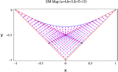
Figure 1: Classical energy-momentum diagram and joint spectrum of two integrals of motion for the Manakov top model (2.1) with $a=4$, $b=3$, $S=T=15$.

Before starting to discuss qualitative features of the concrete problem we need to verify that the chosen problem is generic or structurally stable. In other words we need to verify that any admissible small modification of parameters does not change qualitative features of classical energy momentum diagram and of joint quantum spectrum.

The first initial simplest qualitative characterization of both the EM map image and the foliation is the splitting of the whole image of the EM map into connected regions of regular values. Each region is characterized by the number of connected components (tori) in the inverse image of each regular value.

Fig. 2 shows what happens when we change slightly parameters $a$, $b$ of the model (2.1). We keep, naturally, under such deformation the integrability of the problem and the $S=T$ condition. The image of the EM map becomes less symmetric but it keeps the presence of four regions of regular values and the numbers of connected components in regular inverse images. There are two connected components in regions labeled by I, III, and IV, and four connected components in region II.

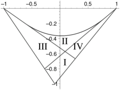
Figure 2: Base of integrable fibration of Manakov top (bifurcation diagram).

As soon as small variation of parameter values $a$, $b$ does not modify the number of regions on the bifurcation diagram the chosen values can be considered as generic. At the same time large variation of the same parameters can lead to qualitatively different bifurcation diagrams. Various possibility are discussed in the appendix. We mention here only one important limiting case corresponding to $(a=2$, $b=1)$. This limiting case is extremely simple because of particular form of two commuting operators $X$, $Y$:

$$X=s_{1}t_{1}+s_{3}t_{3},\qquad Y=-\frac{(s_{2}+t_{2})^{2}}{4}.$$ (3.1)

The corresponding bifurcation diagram is shown in Fig. 3, left. It follows from generic bifurcation diagram (Fig. 2) by shrinking regions II, III, and IV to zero. In this limiting case we have only one region with each internal point corresponding to two connected components (regular tori) in the inverse image.

By going to $Y^{\prime}=\sqrt{-Y}$ we easily recover the integrable fibration with one connected component in the inverse images of any point and the singularity at $Y^{\prime}=X=0$ corresponding in the classical case to doubly pinched torus. The transformation from $\{X,Y\}$ to $\{X,Y^{\prime}=\sqrt{-Y}\}$ can be described as ‘square root unfolding’. It was analyzed in classical mechanics recently [10]. The corresponding transformation of the bifurcation diagram is shown in Fig. 3.

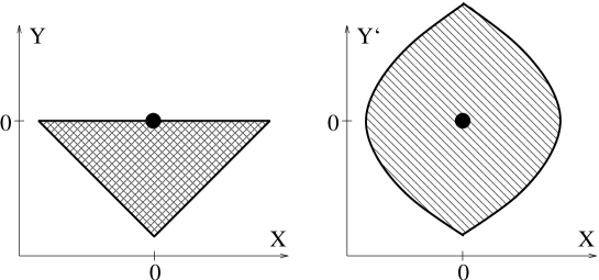
Figure 3: Left: Base of integrable fibration of Manakov top for a special limiting case ($a=2$, $b=1$). Right: Unfolded bifurcation diagram for ($a=2$, $b=1$) Manakov top with $Y^{\prime}=\sqrt{-Y}$.

We make accent in the present paper on the analysis of the quantum problem. But in order to recover the qualitative features of the quantum joint spectrum we need to study it together with the classical bifurcation diagram.

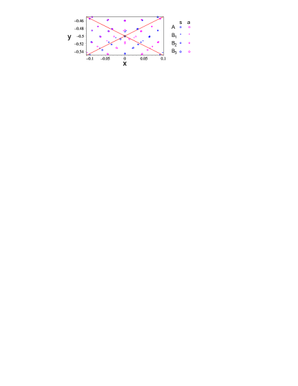
Figure 4: Central part of the joint spectrum of the Manakov top shown in Fig. 1.

The joint spectrum of quantum operators is shown in the same Fig. 1 by different symbols depending on the symmetry of the state. Taking into account the finite symmetry of the problem (see appendix for details) there are quantum states of eight different symmetry types. It is practically impossible to distinguish different symbols on this Fig. 1 because of the overlapping of different symbols due to quasi-degeneracy of eigenvalues. All representations of the symmetry group are one-dimensional, but the quasi-degeneracy is almost perfect in the most part of the region (except neighborhoods of internal singular lines). Thus it is clear that the most prominent qualitative feature of the joint spectrum is its cluster structure. The rearrangement of clusters near singular lines is more clearly seen in Fig. 4 which shows in more details the joint quantum spectrum in the most complicated central part of the energy momentum diagram.

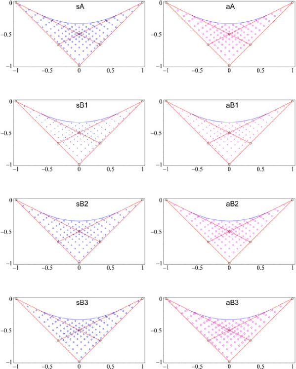
Figure 5: Joint spectrum of Manakov top. Only eigenvalues of one symmetry type are shown on each sub-figure.

We can neglect in the first approximation the internal structure of clusters and try to characterize clusters and to understand their global arrangement. It is quite easy to see that in regions of EM diagram with $K$ connected components for each inverse image, the $K$-fold clusters of quantum eigenvalues should be present. Thus in regions I, III, IV of the EM diagram the 2-fold clusters are present, whereas the region II is filled with the 4-fold clusters. Highly regular pattern formed by the common eigenvalues is clearly seen in Fig. 1. The most part of each of the four regular regions can be regarded as covered with almost regular lattice of 2-fold or 4-fold clusters. By a slight deformation each such lattice can be deformed to a part of an ideal square lattice. Rearrangement of clusters takes place near the lines of singular values of classical EM map and an apparent non-regularity is concentrated near the singular lines (see Fig. 4).

In order to understand the origin of regularity and non-regularity we remind first that the classical phase space of the Manakov top problem is compact and the total number of quantum eigenstates is finite and is determined by quantum numbers $S=T$. The example shown in Fig. 1 corresponds to the choice $S=T=15$. This means that the total number of quantum eigenvalues is $31\times 31=961$. If we denote eight different irreducible representations by $A_{s}$, $A_{a}$, ${B_{i}}_{s}$, ${B_{i}}_{a}$, with $i=1,2,3$, the numbers of eigenvalues of each type of symmetry are: $14\times 15/2=105$ for $A_{a}$, $15\times 16/2=120$ for ${B_{i}}_{s}$, ${B_{i}}_{a}$, $i=1,2,3$, and $16\times 17/2=136$ for $A_{s}$. If now we plot eigenvalues of only one type of the symmetry on the classical energy-momentum diagram the pattern of quantum states turns out to be almost regular in the whole region. Fig. 5 demonstrates this fact for all eight symmetry types. The observation of the regularity of joint spectrum for one symmetry type is based on numerical results and requires further independent explanation.

At the same time if we analyze the total joint spectrum (see Fig. 1) it is clear that in regions I, III, IV (two triangle regions and rhomb region, see appendix) the joint spectrum can be qualitatively described as a regular doubly degenerate lattice of common eigenvalues. Region II (parabola region in the notation of appendix) of the joint spectrum in a similar way can be qualitatively characterized as formed by four-fold degenerate regular lattice of common eigenvalues.

Moreover, pairs of quasi-degenerate eigenvalues form different reducible representations in different regions. In region I the degenerate pairs form $A_{s}+B_{2s}$, $A_{a}+B_{2a}$, $B_{1s}+B_{3s}$, and $B_{1a}+B_{3a}$ representations. Degenerate pairs in region III are $A_{s}+B_{3a}$, $B_{1s}+B_{2a}$, $B_{2s}+B_{1a}$, and $B_{3s}+A_{a}$. In region IV we have $A_{s}+B_{3s}$, $B_{1s}+B_{2s}$, $A_{a}+B_{3a}$, and $B_{1a}+B_{2a}$. The quadruples of eigenvalues in region II are $A_{s}+A_{a}+B_{3s}+B_{3a}$ and $B_{1s}+B_{1a}+B_{2s}+B_{2a}$.

It is clear that the lattices defined in different regions cannot fit together along the singular lines because of different organization of the joint spectrum in different regions and because of different numbers of states of various symmetry types. At the same time the regularity of the joint spectrum for each symmetry type indicates the possibility of the global regular labeling of states of each particular symmetry type. Using such labeling we can try to define the continuous evolution of the properly chosen quantum cell through the quantum joint spectrum along the path which crosses singular lines. This is exactly what is needed in order to define quantum monodromy using approach based on the propagation of the elementary quantum cell. Before doing that we remind shortly in the next section the description of quantum monodromy and its generalizations [15, 24, 28, 29, 36, 37] in terms of the ‘quantum cell’ evolution.

4 Relation to monodromy and its generalizations

Qualitative description of joint spectra of quantum problems associated to some integrable classical models is based on the simultaneous description of defects of regular lattices and on affine structure of classical models.

Presence of singular fibers for classical integrable fibrations leads to the appearance of defects of the lattice of joint eigenvalues in corresponding quantum problem. For an integrable Hamiltonian system with two degrees of freedom the simplest codimension two singularity which generically appears in the bifurcation diagram is the so-called focus-focus singularity. The associated singular fiber is a pinched torus. Several times pinched tori are typically possible under the presence of symmetry. Recent rigorous mathematical description of dynamical problems with such singularities can be found in [18, 31, 33, 34]. More physically based intuitive construction was suggested in [15, 28, 36, 37].

Classical monodromy which is due to the presence of a focus-focus singularity (pinched torus) manifests itself in the corresponding quantum problem in the most clear and transparent way as a transformation of the elementary cell of the lattice formed by the joint eigenvalues of commuting quantum observables after its propagation along a closed path surrounding the singularity. The evolution of an elementary quantum cell is based on the existence of local action-angle variables, whereas the nontrivial monodromy demonstrates the absence of global action-angle variables.

Although the relation between Hamiltonian monodromy and the absence of global action-angle variables [8] was formulated in the well-known papers by Nekhoroshev [22] and Duistermaat [12] about 30 years ago the significant physical applications of hamiltonian monodromy in such simple physical systems as atoms and molecules were found only in the last ten years. Without going into details of physical applications we just cite here several recent papers where important physical applications and citations to other publications can be found [5, 6, 9, 24, 29, 30, 32]. From the mathematical point of view the generalization of monodromy can go in two different directions. One can try to define the evolution of a quantum cell or of bases of homology groups for classical integrable fibrations when the closed path crosses some special singular strata. On this way the notions of fractional monodromy [13, 23, 24] and of bidromy [29, 30] were introduced. Completely another possibility is to study higher obstructions to the existence of the action-angle variables, which are related to the codimension-$K$ singularities with $K\geq 3$ [12]. We does not touch this aspect here. Instead we suggest on the example of the Manakov top the generalization of the monodromy notion to a larger class of dynamical systems (integrable fibrations) which admits the presence of new passable singular strata, associated with fusion or splitting of several connected components of the inverse EM image into one.

5 Quantum monodromy for Manakov top

In this section we formulate new result about propagation of quantum cells along noncontractible paths in the base of integrable singular fibration defined by the Manakov top problem. In order to do that we need first to define the path itself. The main problem here is due to:

1. the presence of two or four connected components of the inverse EM image in different regular regions of bifurcation diagram;

2. the continuation of the path when crossing singular strata.

We start with a simple limiting case $a=2$, $b=1$ of the Manakov top problem. Corresponding classical integrable fibration is represented by its bifurcation diagram in $\{X,Y\}$ variables in Figs. 3, left and 6, left. This fibration has two components of the inverse EM image for all regular values. At the same time the inverse image of each of singular values on $(CF)$ and $(FB)$ intervals is one regular torus. Such structure gives possibility to unfold the picture by going from $\{X,Y\}$ to $\{X,Y^{\prime}=\sqrt{-Y}\}$ variables [10]. The closed path in the unfolded variables $\{X,Y^{\prime}\}$ (see Fig. 6, right) encircles the isolated singular value (point $F$) whose inverse image is a doubly pinched torus. Continuous evolution of classical fibers and of corresponding quantum cell along such contour should necessarily lead to nontrivial monodromy [10]. We demonstrate this below on the joint spectrum of this particular example. For a moment we just stress the representation of the closed path in the original variables $\{X,Y\}$ in Fig. 6, left.

Figure 6: Choice of the closed path on the base space for the limiting case $a=2$, $b=1$ of the Manakov top. Left: Representation in $\{X,Y\}$ variables with two components of the inverse image for each regular point. Solid and dashed lines represent parts of the path which belong to different leafs of the unfolded diagram. Right: Representation in $\{X,Y^{\prime}=\sqrt{-Y}\}$ variables with one component of the inverse image for any regular point.

When constructing the closed path on the base of the classical foliation of the generic Manakov top (see Fig. 7) we need to remind that in the internal points of regions $AFDE$, $CDF$, and $AFB$ (regions I, III, IV, in Fig. 2 respectively) the inverse image of the EM map has two connected components, whereas in the internal points of region $KLF$ (region II in Fig. 2) there are four components. At intervals $DF$ and $FA$ each point has one connected component in its inverse image. At the same time at the boundary $LBAEDCK$ there are two components except for points $A$ and $D$. Intervals $KF$ and $FL$ are associated with singular fibers corresponding to splitting of each connected component presented for internal points in regions $AFB$ and $CDF$ into two regular components in region $KLF$.

Figure 7: Choice of the generalized closed path on the base space for the generic Manakov top problem.

We start the path at point $a$ in the ‘rhomb’ region $AFDE$ (region I), see Fig. 7. As soon as there are two connected components in the inverse image, we need to distinguish them and to precise that the point $a$ belongs to one of these components, say to leaf I₁. Alternatively, we can choose starting point $a^{\prime}$ at another leaf I₂. Two different paths associated with different components are represented in Fig. 7 by solid and dash lines.

When going through the point $b\in(DF)$ two components fuse together and split again into two components of the region III, which we denote as III₁, and III₂. Crossing singular stratum $DF$ needs further analysis. We suppose for a moment that at point $b$ we can follow the path continuously from I₁ to III₁ and in a similar way from I₂ to III₂. The intuitive arguments for such continuation will be given below on the basis of the analysis of the evolution of quantum joint spectrum in the neighborhood of singular stratum $DF$.

Next essential step is the crossing the singular stratum $KF$. When crossing this stratum one component splits into two connected components and one regular torus transforms into two regular tori. Similar situation was studied recently by Sadovskii and Zhilinskii [30], who introduced the notion of ‘bidromy’ and the associated notion of ‘bipath’ when crossing the singular stratum corresponding to splitting of one regular component into two components. In a similar way the path which is defined in the region III and follows the component III₁ splits into two-component-path when entering region IV by crossing singular stratum $KF$. This transformation is represented in Fig. 7 by going from single solid line to double solid line after crossing $KF$. Analogous but independent transformation takes place for the path defined in region III for the component III₂ (dash line in Fig. 7).

Further continuation through singular strata $FL$ and $AF$ enables us to define the closed path starting at point $a$ on component I₁ and ending at the same point. Again the intuitive justification of the construction of such generalized closed path is given below on the basis of the evolution of ‘quantum cells’ through the joint spectrum of mutually commuting quantum operators for Manakov top problem.

Obvious difficulty in proper definition of the corresponding classical (quantum) construction for such generalized closed path is related to the definition of the connection between bases of the homology groups (or appropriate subgroups) of regular fibers when the path crosses singular strata. In this article we do not want to discuss this delicate question and leave the description of the classical problem open for further study. In contrast, we concentrate on the quantum problem and demonstrate below how quantum mechanical results allow to introduce the continuous evolution of the quantum cell through singular strata and to define the quantum monodromy for the Manakov top.

We hope that the quantum aspect can stimulate further analysis of corresponding classical problem which will probably lead to another generalization of the classical Hamiltonian monodromy concept in a way similar to appearance of classical fractional Hamiltonian monodromy stimulated by initial quantum conjectures.

The key point in the construction of the evolution of the quantum cell through the joint spectrum is the regularity of the pattern of common eigenvalues of two commuting operators formed by eigenvalues with one chosen symmetry type. It is useful to remind here that in almost all standard problems with Hamiltonian monodromy one of the integrals is related to continuous symmetry and is a good global action variable by construction. In such a case splitting the total set of common eigenvalues into subsets with different symmetry types leads from 2D-pattern for the total problem to a family of 1D-patterns for different symmetry types. In order to see monodromy we are obliged to compare common eigenvalues with different continuous symmetry (different values of angular momentum, for example). Fractional monodromy also follows naturally this kind of reasoning. Looking at two sub-lattices separately (for problems possessing half-integer monodromy) does not allow to see the phenomenon (see detailed discussion in [24]). In order to observe the half-integer monodromy we are obliged to analyze two (index two) sub-lattices simultaneously.

The Manakov top problem possesses finite symmetry group which allows classification of the common eigenvalues of operators $X$ and $Y$ by eight different irreducible representations. This allows us to make a choice of elementary quantum cell in the region I as formed by four different eigenvalues.

Before going to the analysis of the evolution of quantum cell for generic Manakov top problem we study first one particular limiting case $a=2$, $b=1$ (see equations (3.1) and Figs. 3, 6) of the Manakov top problem.

5.1 Quantum cell evolution for particular limiting case

The particular case $a=2$, $b=1$ of the Manakov top problem is especially simple because of a possibility of a ‘square root unfolding’ [10] by going to new commuting variables $X=s_{1}t_{1}+s_{3}t_{3}$, $Y^{\prime}=\sqrt{-Y}=(s_{2}+t_{2})/2$.

The evolution of the elementary quantum cell through the joint spectrum of $X$, $Y^{\prime}$ becomes simple because $Y^{\prime}$ is the generator of a global continuous symmetry, the projection of the total momentum on axis 2. In classical mechanics $Y^{\prime}$ can be used as a global action. Second global action does not exist for this problem due to presence of an isolated critical value $X=Y^{\prime}=0$. Fig. 8 clearly shows that the monodromy matrix corresponding to the transformation of the elementary cell along a closed path encircling the critical value in the chosen basis of the joint spectrum lattice has the form $\left(\begin{matrix}1&0\\ 2&1\end{matrix}\right)$.

It is useful to go back to original $\{X,Y\}$ variables and to represent the evolution of the quantum cell along the same closed path but in $X$, $Y$ variables as in Fig. 6, left.

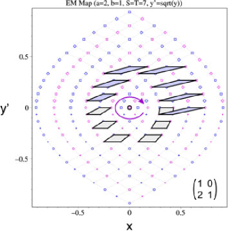
Figure 8: Joint spectrum of commuting quantum operators $X,Y^{\prime}=\sqrt{-Y}$ for the limiting case $a=2$, $b=1$ of the Manakov top together with the evolution of the elementary quantum cell along a closed path encircling critical value $X=Y^{\prime}=0$.

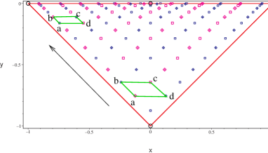
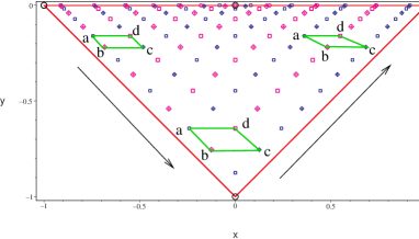
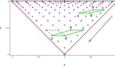
Figure 9: ‘Parallel transport’ of an elementary quantum cell along the closed path surrounding central singularity for the special limiting case of Manakov top (2.1) with $a=2$, $b=1$.

The symmetry of the $a=2$, $b=1$ case is higher than the symmetry of a generic Manakov top problem. Thus we can still use eight irreducible representations of the initially chosen symmetry group to label the common eigenvalues even when they belong to doubly degenerate representations of higher symmetry group. We split eight irreducible representations of the initial symmetry group into two different groups and associate each group with its own leaf on the EM diagram. In such a case we start at Fig. 9 (upper sub-figure) with an elementary cell formed by four different representations and associated with one leaf. We move the cell towards $Y=0$ stratum and cross it (using $Y^{\prime}$ unfolded coordinates) changing at the same time the irreducible representations associated with the vertices of the cell. Further evolution (Fig. 9, middle) is done on the second leaf. Then passing again through the $Y=0$ stratum we return back to the first leaf and can compare final cell with the initial one.

Naturally, the transformation of the cell along the closed path depends on the choice of the basis. Two alternative choices of the lattice basis are used in Fig. 10 to illustrate the monodromy transformation. It is well known that the matrix representation of the monodromy transformation depends on the lattice basis and is defined up to similarity transformation with a matrix from $SL(2,Z)$ corresponding to basis transformation of regular lattice. For two examples shown in Fig. 10 the matrix of the monodromy transformation can be easily written in an algebraic form. For one case (lower in Fig. 10) we have

$$ad\rightarrow ad;\qquad ab\rightarrow ab+2ad,$$

and the corresponding matrix is $\left(\begin{matrix}1&0\\ 2&1\end{matrix}\right)$. Alternative choice of the basis shown on the same figure gives

$$ad\rightarrow-2ab-ad;\qquad ab\rightarrow 3ab+2ad,$$

and the corresponding matrix is $\left(\begin{matrix}3&2\\ -2&-1\end{matrix}\right)$.

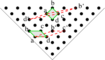
Figure 10: Transformation of the cell after parallel transport along closed path represented in Fig. 6. Two different choices of an elementary cell are shown. Initial cells are shown by solid line. Final cells are shown by dash line.

5.2 Evolution of quantum cell for generic Manakov top problem

For the generic Manakov top problem in order to realize the evolution of the quantum cell along the closed path shown in Fig. 7 we need to study crossing two different singular strata.

Let us start with crossing $DF$ (or $AF$) stratum. We make the choice of an elementary quantum cells in region I as formed by four eigenvalues of different symmetry $(A_{s},A_{a},B_{1s},B_{1a})$, associated with leaf 1. Four other symmetry types $(B_{2s},B_{2a},B_{3s},B_{3a})$ are associated with another leaf.

The splitting of eight different representations into two groups of four is unique because we impose the requirement that after the evolution of all vertices of the cell into region III or region IV the elementary cell should remain elementary, i.e. vertices should not belong, for example, to the pair of degenerate eigenvalues. The evolution of eigenvalues of each symmetry type is realized using the correspondence between the joint spectrum lattice formed by states of one symmetry type and the part of the regular square lattice having the form of an equilateral rectangular triangle. Such correspondence is global and it enables us to go through the singular stratum $DF$ or $AF$ (point $b$ or $e$ in Fig. 7).

         

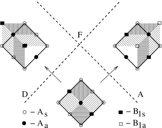
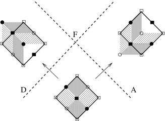
Figure 11: Transformation of quantum cell under crossing singular strata $DF$ and $AF$ (see Fig. 6). Elementary cells are shown by different hatching. Two alternative choices of big ‘quadruple’ cell are shown. Left: Cell is formed by $A_{s}$ vertices. Right: Cell is formed by $B_{1a}$ vertices.

Fig. 11 shows that different elementary cells transforms after crossing singular stratum in different way. Saying in another way, this singular stratum is not passable by an elementary cell. Nevertheless, one can choose bigger cells which pass through singular stratum unambiguously. The situation here is similar to the fractional $1/2$ monodromy, where elementary cell cannot pass but the double cell passes. At the same time, the case of Manakov top is slightly different. In order to pass through $DF$ stratum the cell should be doubled in the direction parallel to $DF$, whereas to pass through $AF$ stratum the cell should be doubled in the direction parallel to $AF$ which is orthogonal to $DF$ from the point of view of regular lattice in the region I. The conclusion: In order to pass through both $DF$ and $AF$ the cell should be quadruple in such a way that all its vertices correspond to the same irreducible representation. Fig. 11 shows evolution of two such quadruple cells (with vertices of $A_{s}$ and of $B_{1a}$ symmetry respectively). Similar modifications take place for all other cells which can be defined on both leafs in the region I.

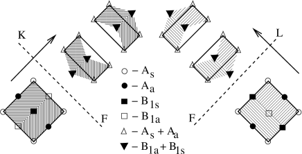
Figure 12: Transformation of quantum cells under crossing singular strata $DF$ and $AF$ (see Fig. 6). Minimal (double elementary) cells are shown by different hatching. Big ‘quadruple’ cell consists of two minimal cells. It splits into two cells which belong to different leafs in region II.

The situation with crossing singular strata $KF$ and $FL$ is quite different from crossing $DF$ or $FA$ strata. Entering region II is associated with splitting of one connected component of the classical fibration into two. The associated transformation of quantum cell is the splitting of one cell into two. The natural physical requirement imposed on such transformation is the conservation of the reduced volume [30], i.e. the volume of the cell in the local action variables. This means that in order to pass through the $KF$ line from region III to region II, for example, the initial cell should be at least double. After crossing $KF$ line it splits in this case into two single cells associated with two different leafs in region II. These two different cells can be moved through region II along two-component path represented in Fig. 7.

Fig. 12 shows transformation of quantum cells when they cross the singular stratum $KF$ and $FL$. The first important observation is that two double cells (formed each by two elementary cells in region III and shown by different hatching) leads to different pairs of single cells in region II. This means that the minimal cell should be doubled once more in order to define an unambiguous transformation of the quantum cell after crossing singular $KF$ stratum. The quadruple cell chosen in regions III as having vertices of the same symmetry splits into two double cells in region II in a unique way. The situation is completely similar with crossing $FL$ stratum.

Reverse transformation from region II to region III or IV through singular $KF$ or $FL$ strata leads to fusion of two double cells into one quadruple cell.

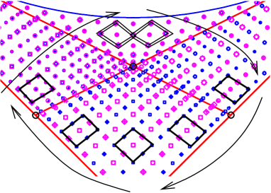
Figure 13: Transformation of quantum cell along a closed path (see Fig. 7). Quadruple cell chosen in region I remains quadruple in region III, splits into two double cells entering into region II, fuses again into quadruple cell returning back to region IV and to region I.

Now, we can realize the evolution of the quantum cell along the closed path represented in Fig. 7. We present in Fig. 13 such evolution using the essential part of the joint spectrum of the Manakov problem for $a=4$, $b=3$, $S=T=15$ (compare with total joint spectrum shown in Fig. 1). It should be noted that we need to follow the evolution of two initial cells. In the region I one of these cells belongs to leaf I₁, while another belongs to leaf I₂. But as soon as evolution of both cells is completely similar except for the fact that the cells follow different leafs, we can discuss only the case of the cell located on the leaf I₁. The initial cell consists of four elementary cells in the region I. It has all its vertices labeled by the same irreducible representation and it is associated with the leaf I₁. We follow further the path represented in Fig. 7 by solid line. The cell can cross the singular stratum $DF$ and to move further through leaf III₁ till singular stratum $KF$.

When crossing $KF$ stratum the quadruple cell transforms into two double cells located at two different leafs in region II. We denote these leafs as II_1a and II_1b and remind that there are four different leafs in the region II. The notation we use is based on the fact that the leaf III_i, $(i=1,2)$ splits under crossing $KF$ into two leafs II_ia and II_ib. In a similar way the leaf IV_i splits under crossing $FL$ into two leafs II_ia and II_ib.

Thus in the region II instead of one quadruple cell we have two double cells which are shown superimposed in Fig. 13. These two double cells can be moved through the region II with each cell following its proper leaf. When crossing $FL$ singular stratum the two cells fuse together and form one quadruple cell located at the leaf IV₁. This cell moves further towards the singular stratum $FA$, crosses it and returns back on the leaf I₁ to the initial position.

Exactly the same transformation takes place for the initial quadruple cell chosen in region I at leaf I₂. In both cases the transformation between initial and final cell is trivial, i.e. the monodromy matrix is identity. The non-triviality of such transformation is due to the fact that only quadruple cells are passable and the path along which the cell is propagated has two branching points where the path bifurcates into two-component path and fuse from two-component path back into one-component path.

It is quite interesting to compare the present situation with the analysis of the $1:2$ [7] and $1:(-2)$ [24] resonant nonlinear oscillators. Both these problems have one-dimensional singular stratum in the image of the momentum map which is formed by points with inverse image being ‘curled torus’ [7, 24]. This stratum is not passable in quantum version by an ‘elementary cell’ but it is passable by ‘double cell’. $1:2$ resonance problem has no nontrivial monodromy because there is no non-contractible circular paths due to the fact that the line of critical values ends at the boundary and the end point cannot be encircled. In contrast the $1:(-2)$ problem [24] has singular stratum with the end point and the nontrivial fractional monodromy could be introduced with that example. Probably the present discussion of the quantum Manakov top will stimulate looking for further examples of integrable systems with still less trivial but generic behavior in classical and quantum systems.

6 Conclusions

The analysis of the possible propagation of the quantum cell through the joint quantum spectrum of two commuting observables for the Manakov top model is studied in this paper for the first time. The presentation of the material here is done on completely heuristic physical ground. Nevertheless, the authors hope that our result about quantum monodromy will find more serious description in classical as well as in quantum mechanics. We believe that further analysis will lead to the formulation of new important qualitative features of classical and quantum problems and allow to make further important steps in formulating general qualitative theory of highly excited quantum systems which is the ultimate goal of the authors.

Appendix A Symmetry group action on the phase space

The first step in the qualitative analysis of any given model problem is the analysis of the symmetry group action on the dynamical variables. Below we follow general ideas of the group theoretical and topological analysis of molecular models outlined in [21, 35].

Fixing Casimirs $S=T>0$ we obtain direct product of two $S_{2}$ spheres as a phase space of the classical Manakov top.

Now we want to find the stratification of this space under the symmetry group action. For model in question the symmetry group $G$ consists of two subgroups. One, which we denote $D_{2h}$ using standard Schönflies notation, acts in natural diagonal way on two $S$ and $T$ spheres. Another subgroup is the permutation of appropriate points on $S$ and $T$ spheres, $P_{st}$, which acts as $s_{i}\leftrightarrow t_{i}$. The total group is $D_{2h}\wedge P_{st}$. The diagonal action of $D_{2h}$ on two spheres $S$ and $T$ is shown on Fig. 14. On every sphere we have three one dimensional invariant manifolds (bold circles) with $C_{s}^{(ij)}$ stabilizers ($C_{s}^{(ij)}$ is an order two group generated by the reflection in the plane passing through axes $i$ and $j$). Three pairs of diametrically opposite points of intersections of circles form three zero dimensional strata with $C_{2v}^{(j)}$ stabilizers ($C_{2v}^{(j)}$ is an order four group generated by two reflections in planes $ij$ and $jk$). All the remaining points on the spheres have a trivial stabilizer 1 and so belong to principal type of orbits (orbits that consist of regular points). The isolated points of the group action, i.e.  points with local symmetry (stabilizer) different from local symmetries of all other neighboring points, form critical orbits. By the theorem of Michel [20, 21] the gradient of every $G$-invariant function vanishes on critical orbits. As a consequence, certain stationary points of invariant functions can be found using only symmetry group action rather than the concrete form of functions.

   

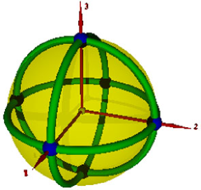
Figure 14: Diagonal action of $D_{2h}$ group on $S$ and $T$ spheres.

To determine the nontrivial invariant subspaces of $D_{2h}$ group in full four dimensional space we need to look for products of subspaces on $S$ and $T$ spheres which have nontrivial intersections of their stabilizers. For example let’s take the point with local symmetry $C_{2v}^{(1)}$ on $S$ sphere, then on $T$ sphere we must take the point with the same stabilizer in order to obtain an orbit of critical points in four dimensional space. Different combinations of points on $S$ and $T$ spheres give us a family of two critical orbits (each formed of two points) in the full space. All resulting zero dimensional strata of the Manakov top phase space are listed in Table 1. Points of the same orbit are denoted by one letter. They are further distinguished by indices.

Table 1: Isolated points and their stabilizers.

Point	$s_{1}$	$s_{2}$	$s_{3}$	$t_{1}$	$t_{2}$	$t_{3}$	Stabilizer 2pt1pt
$B_{2}$	$\phantom{-}1$	0	0	$\phantom{-}1$	0	0	$C_{2v}^{(1)}\wedge P_{st}$ 6pt
$B_{1}$	$-1$	0	0	$-1$	0	0
$C_{2}$	$\phantom{-}1$	0	0	$-1$	0	0	$C_{2v}^{(1)}\wedge P_{st}\sigma^{23}$
$C_{1}$	$-1$	0	0	$\phantom{-}1$	0	0
$E_{1}$	0	$\phantom{-}1$	0	0	$\phantom{-}1$	0	$C_{2v}^{(2)}\wedge P_{st}$
$E_{2}$	0	$-1$	0	0	$-1$	0
$F_{1}$	0	$\phantom{-}1$	0	0	$-1$	0	$C_{2v}^{(2)}\wedge P_{st}\sigma^{13}$
$F_{2}$	0	$-1$	0	0	$\phantom{-}1$	0
$A_{1}$	0	0	$\phantom{-}1$	0	0	$\phantom{-}1$	$C_{2v}^{(3)}\wedge P_{st}$
$A_{2}$	0	0	$-1$	0	0	$-1$
$D_{1}$	0	0	$\phantom{-}1$	0	0	$-1$	$C_{2v}^{(3)}\wedge P_{st}\sigma^{12}$
$D_{2}$	0	0	$-1$	0	0	$\phantom{-}1$

Taking now invariant circles on $S$ and $T$ spheres with the same stabilizer we can form in the 4-dimensional space their products. This gives invariant tori $T_{i}(s_{1},s_{2},s_{3},t_{1},t_{2},t_{3})$ in $S_{s}^{2}\otimes S_{t}^{2}$ (their stabilizers are given in the right column):

$$T_{1}(0,s_{2},s_{3},0,t_{2},t_{3}),\qquad G_{T_{1}}=\{E,\sigma^{23}\},$$

$$T_{2}(s_{1},0,s_{3},t_{1},0,t_{3}),\qquad G_{T_{2}}=\{E,\sigma^{13}\},$$

$$T_{3}(s_{1},s_{2},0,t_{1},t_{2},0),\qquad G_{T_{3}}=\{E,\sigma^{12}\}.$$

As soon as each basic circle of each torus has four points of higher symmetry each torus itself contains eight isolated (by local symmetry) points. All twelve isolated points are listed in Table 1. The number of $G$-invariant tori is three and on each of them there are eight points whereas in Table 1 we have only twelve points. This means that every point belongs to two tori, or, in other words, every isolated point on a torus is a common point with another torus.

Finally, acting by $D_{2h}$ group on Manakov top phase space we obtain three invariant subspaces. They are tori which have isolated points on them in such a way that each torus has four common points with each of two other tori.

To complete the analysis of the symmetry group action on the classical phase space we need to consider the action of the permutations of $s$ and $t$ components on the full space and on the $G$-invariant tori in particular. In full space the action of operations $P_{st}g$ ($g\in D_{2h}$) gives eight invariant subspaces $S_{i}(s_{1},s_{2},s_{3},t_{1},t_{2},t_{3})$ (for further convenience we call them $G$-invariant spheres):

$$S_{1}(\alpha,\beta,\gamma,\alpha,\beta,\gamma),\qquad G_{S_{1}}=\{E,P_{st}\},\qquad {\rm dynamically\;invariant},$$

$$S_{2}(\alpha,\beta,\gamma,\alpha,\beta,-\gamma),\qquad G_{S_{2}}=\{E,P_{st}\sigma^{12}\},$$

$$S_{3}(\alpha,\beta,\gamma,\alpha,-\beta,\gamma),\qquad G_{S_{3}}=\{E,P_{st}\sigma^{13}\},$$

$$S_{4}(\alpha,\beta,\gamma,-\alpha,\beta,\gamma),\qquad G_{S_{4}}=\{E,P_{st}\sigma^{23}\},$$

$$S_{5}(\alpha,\beta,\gamma,\alpha,-\beta,-\gamma),\qquad G_{S_{5}}=\{E,P_{st}C_{2}^{(1)}\},\qquad {\rm dynamically\;invariant},$$

$$S_{6}(\alpha,\beta,\gamma,-\alpha,\beta,-\gamma),\qquad G_{S_{6}}=\{E,P_{st}C_{2}^{(2)}\},\qquad {\rm dynamically\;invariant},$$

$$S_{7}(\alpha,\beta,\gamma,-\alpha,-\beta,\gamma),\qquad G_{S_{7}}=\{E,P_{st}C_{2}^{(3)}\},\qquad {\rm dynamically\;invariant},$$

$$S_{8}(\alpha,\beta,\gamma,-\alpha,-\beta,-\gamma),\qquad G_{S_{8}}=\{E,P_{st}I\}.$$ (A.1)

In order to describe the group action we introduce on each torus angle variables:

$$T_{i}:\qquad s_{i}=0,\qquad s_{j}=\cos\phi_{s},\qquad s_{k}=\sin\phi_{s},$$

$$t_{i}=0,\qquad t_{j}=\cos\phi_{t},\qquad t_{k}=\sin\phi_{t}.$$ (A.2)

The action of $P_{st}g$ on $\phi_{s}$ and $\phi_{t}$ is shown for $T_{2}(s_{1},s_{3},t_{1},t_{3})$ in Table 2. Fourth column indicates four different relations between angle coordinates on torus resulting in points with higher symmetry. This symmetry group is given in the last column. The indicated lines pass throw the isolated points on the torus.

By comparing the stabilizers of lines (Table 2) and that of isolated points (Table 1) it is easy to conclude what line contains what points. Moreover, the intersections of line stabilizers with stabilizers of $G$-invariant spheres (A.1) are also nontrivial. This means that all points of the line $\phi_{s}=\phi_{t}$, for example, at the same time belong to $S_{1}$ ($G_{S_{1}}\cap G_{(\phi_{s}=\phi_{t})}\neq\{E\}$) and $S_{3}$ ($G_{S_{3}}\cap G_{(\phi_{s}=\phi_{t})}\neq\{E\}$) invariant subspaces, the line $\phi_{s}=-\phi_{t}$ belongs to $S_{2}$ and $S_{5}$ invariant subspaces and so on. The construction of tables equivalent to Table 2 for $T_{1}$ and $T_{3}$ shows that the line equations are the same:

$$\phi_{s}=\phi_{t},\qquad\phi_{s}=-\phi_{t},\qquad\phi_{s}=\pi-\phi_{t},\qquad\phi_{s}=\pi+\phi_{t},$$ (A.3)

but the stabilizers are different. Subsequently, every line (A.3) on a torus is an intersection line of this torus with two spheres (one of these spheres is dynamically invariant) and every torus has lines of intersections with all $G$-invariant spheres.

Table 2: Action of $P_{st}g$, ($g\in D_{2h}$) on $T_{2}$.

Operator	Action on $\{s_{i},t_{i}\}$		Line Equation	Stabilizer of Line 2pt1pt
$P_{st}$	$s_{1}=t_{1}$	$s_{3}=t_{3}$	$\phi_{s}=\phi_{t}$	$\{E,\sigma^{13},P_{st},P_{st}\sigma^{13}\}$4pt
$P_{st}\sigma^{13}$	$s_{1}=t_{1}$	$s_{3}=t_{3}$	$\phi_{s}=\phi_{t}$
$P_{st}\sigma^{12}$	$s_{1}=t_{1}$	$s_{3}=-t_{3}$	$\phi_{s}=-\phi_{t}$	$\{E,\sigma^{13},P_{st}\sigma^{12},P_{st}C_{2}^{(1)}\}$
$P_{st}C_{2}^{(1)}$	$s_{1}=t_{1}$	$s_{3}=-t_{3}$	$\phi_{s}=-\phi_{t}$
$P_{st}\sigma^{23}$	$s_{1}=-t_{1}$	$s_{3}=t_{3}$	$\phi_{s}=\pi-\phi_{t}$	$\{E,\sigma^{13},P_{st}\sigma^{23},P_{st}C_{2}^{(3)}\}$
$P_{st}C_{2}^{(3)}$	$s_{1}=-t_{1}$	$s_{3}=t_{3}$	$\phi_{s}=\pi-\phi_{t}$
$P_{st}C_{2}^{(2)}$	$s_{1}=-t_{1}$	$s_{3}=-t_{3}$	$\phi_{s}=\pi+\phi_{t}$	$\{E,\sigma^{13},P_{st}C_{2}^{(2)},P_{st}I\}$
$P_{st}I$	$s_{1}=-t_{1}$	$s_{3}=-t_{3}$	$\phi_{s}=\pi+\phi_{t}$

Figure 15: Stratification of invariant tori. Representation of $T_{1}$, $T_{2}$ and $T_{3}$ (from left to right). Zero-dimensional strata together with their stabilizers are given in Table 1. One-dimensional strata are listed in Table 2 for one of the torus, $T_{2}$. The construction is similar for two other tori.

Thus the stratification of the Manakov-top phase space under the action of $D_{2h}\wedge P_{st}$ group is constructed. In particular, the system of isolated critical orbits which is due to the symmetry group action is given. All points forming these orbits are stationary points of any invariant function [20, 21]. This result is in fact independent on the concrete form of integrals of motion and relies only on symmetry arguments. Such preliminary symmetry analysis is quite important in the qualitative study of molecular models as it is formulated in our previous works [27, 21, 35, 14].

Appendix B Critical points of energy-momentum map

In this section we find critical points of the energy momentum map defined on the classical phase space of the Manakov top by two integrals of motion $X$, $Y$ given in equation (2.1). By definition, the point is critical, if the differentials of two integrals of motion, $dX$ and $dY$ are linearly dependent, or equivalently the corresponding matrix of derivatives has non-maximal rank. We can greatly simplify the problem of searching critical points by restricting differentials on the symmetry invariant sub-manifolds.

For $G$-invariant tori with coordinates (A.2) the condition of non-maximal rank is

$${\rm det}\left(\begin{matrix}\dfrac{\partial X}{\partial\phi_{s}}&\dfrac{\partial X}{\partial\phi_{t}}\\[8.61108pt] \dfrac{\partial Y}{\partial\phi_{s}}&\dfrac{\partial Y}{\partial\phi_{t}}\end{matrix}\right)=0.$$ (B.1)

The solution of equation (B.1) has for every torus ($T_{1},T_{2}$, or $T_{3}$) six roots. Four of them are, naturally, the lines (A.3)

$$s=\biggl{\{}t,-t,\frac{1}{t},-\frac{1}{t}\biggr{\}},$$

which have the same form for $T_{1}$, $T_{2}$, $T_{3}$. These lines are shown in Fig. 15. They are completely defined by the symmetry group action and do not depend nor on values of $a$ and $b$ parameters nor on the choice of invariant functions defined on $S_{s}^{2}\otimes S_{t}^{2}$. Two others roots are curves which depend on the concrete form of functions $X$ and $Y$ specified by parameters $a$, $b$. Their analytic form varies slightly with invariant torus as follows:

$$T_{1}:\quad s=\frac{(a-b-1)t\pm\sqrt{a(1-b)(t^{4}-1)+2(2b-a(1+b))t^{2}}}{at^{2}+b-1},$$

$$T_{2}:\quad s=\frac{(a+b-1)t\pm\sqrt{(a-b)(t^{4}+1)+2(b(a-1)+a(b-1))t^{2}}}{-t^{2}+a-b},$$

$$T_{3}:\quad s=\frac{(1-a-b)t\pm\sqrt{(b-a)(t^{4}+1)+2(b(a-1)+a(b-1))t^{2}}}{t^{2}+a-b}.$$ (B.2)

Here $s=\tan(\phi_{s}/2)$ and $t=\tan(\phi_{t}/2)$. The form and position of curves (B.2) on tori $T_{i}$ depend on $a$ and $b$. For the parameters values $a>b>1$ only two curves from (B.2), namely curves defined for $T_{2}$ and $T_{3}$ tori, have a real range of values, they are shown on Fig. 16.

   

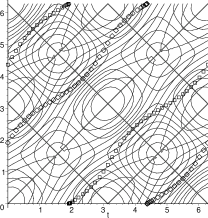
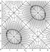
Figure 16: Affine charts of tori 2 and 3 with level lines of $X$ and $Y$ ($a=4$, $b=2$). Critical curves (B.2) are shown by box and diamond points.

Similar construction of matrix for $dX$ and $dY$ for $G$-invariant spheres gives us the matrix with determinant identically equal to zero (rank of the matrix is less then two). The rank of this matrix equals identically zero in all points which belong to critical orbits listed in Table 1. In all other points of the $G$-invariant spheres the rank of the matrix equals one. This means that there are no other critical points on spheres except those isolated points found earlier from the symmetry considerations.

Appendix C Classical energy momentum map

The set of two integrals $F=\{X,Y\}$ (2.1) defines the mapping $F:S_{s}^{2}\otimes S_{t}^{2}\rightarrow R^{2}$. Possible values $f\in R^{2}$ of the map form the image of the map, or the base of the corresponding integrable fibration. We distinguish regular and critical values of the map. The set of critical values forms what is often called the bifurcation diagram. Below, we call the set of all, regular and critical values of EM map an energy-momentum diagram. In this section we discuss the form of the energy-momentum diagram for one particular choice of parameters $a$, $b$ and its variation along the modification of parameters.

Let us first take parameters $a$, $b$ in (2.1) as

$$a>b>1,$$ (C.1)

and find images of critical points of rank zero (Table 1). Substitution of their coordinates into equation (2.1) confirms that every point from one symmetry group orbit naturally gives the same value of functions $X$ and $Y$, so we have six critical values of EM map specified below by their coordinates in $R^{2}$ plane of $(X,Y)$ values:

$$B(1,0),\qquad C(-1,0),$$

$$E\biggl{(}\frac{a-b-1}{1-a-b},\frac{-4ab(1-a)}{1-a-b}\biggr{)},\qquad F\biggl{(}-\frac{a-b-1}{1-a-b},\frac{4b(1-a)(1-b)}{1-a-b}\biggr{)},$$

$$A\biggl{(}\frac{b-a-1}{1-a-b},\frac{-4ab(1-b)}{1-a-b}\biggr{)},\qquad D\biggl{(}-\frac{b-a-1}{1-a-b},\frac{4a(1-a)(1-b)}{1-a-b}\biggr{)}.$$

Points $B$, $C$ do not depend on $a$, $b$ parameters. For the choice of parameters as in equation (C.1), the $x$ component for all other points always lie in the $[-1,1]$ region and $y$ component is always negative.

Next we construct the images under the EM map of $G$-invariant tori (for $T_{i}$ we have $s_{i}=t_{i}=0$). In Fig. 17 the colored regions correspond to images of regular points on tori, the bold lines are the images of critical lines on tori. As it was mentioned earlier, for the given choice of $a$, $b$ parameters the curves (B.2) exist only for two tori. On the EM diagram the image of these curves is represented as a part of parabola. We will call the neighboring area having the form of a small curved triangle the parabola area.

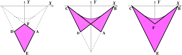
Figure 17: Images of $T_{1}$, $T_{2}$ and $T_{3}$ tori under the EM map. Images of zero rank points on tori are denoted by Latin letters.

Images of lines of critical points on tori (A.3) associated with linear dependence between $dX$ and $dY$ can be written explicitly as

$$Y=2ab(X-1),\qquad Y=2a(1-a)(X+1),$$

$$Y=2(1-a)(1-b)(X-1),\qquad Y=2b(1-b)(X+1).$$

Explicit form for the boundary of the parabola region is simple only for a certain choices of $a$ and $b$, for example for $a-b=1$ when the EM diagram has a symmetric form like that on Fig. 17.

The images of four $G$-invariant spheres belong to critical lines (A.3), they are shown on the most left sub-figure of Fig. 18. Each of these lines is denoted by $L_{i}$ with its index corresponding to a dynamical sphere $S_{i}$, $i\in\{1,5,6,7\}$. All other $S_{i}$ $i\in\{2,3,4,8\}$ are mapped to 2-D triangular regions in $\cal{EM}$ diagram formed by regular values and bounded by lines of critical values.

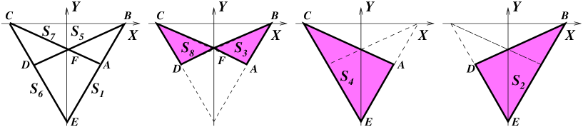
Figure 18: Images of the $G$-invariant spheres. First figure on the left represent four dynamically $G$-invariant spheres having 1D-images (straight lines).

So the boundaries of the image of EM map of Manakov top for some particular choice of parameters $a$, $b$ are formed by four straight lines and one parabola. There are four areas: area of parabola (II), two triangles (III, IV) and a rhomb (I) (Fig. 2). Two lines always pass through the fixed point $(-1,0)$ ($L_{6}$ and $L_{7}$) and two other lines always pass through point $(1,0)$ ($L_{1}$ and $L_{5}$). When both parameters are of the same sign, $Y$ function is negative and takes the zero values only in mentioned points.

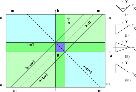
Figure 19: ‘Critical’ values of $a$ and $b$ parameters (left). Right figures are the limiting cases corresponding to $a\rightarrow\infty$ and to : i) $b=a-1$, ii) $a-1>b\geq 1$, iii) $1>b>0$, iiii) $0\geq b>-a+1$.

Now we will summarize briefly the dependence of the bifurcation diagram on the values of $a$ and $b$ parameters. In the space of $a$, $b$ parameters there are regular values corresponding to qualitatively the same generic diagram formed by four straight lines and one parabola. Critical values of $a$, $b$ parameters correspond to some degenerate situations when the image of the EM map qualitatively changes, i.e. some regions shrink to zero and some lines coincide. Moreover, there is some symmetry in the space of $a$, $b$ parameters which enables one to study only part of the whole plane to recover all the qualitatively different cases of bifurcation diagrams. Fig. 19 which can be named with some abuse of the language as a ‘bifurcation diagram of the Manakov-top-bifurcation-diagram’ illustrates the symmetry in the parameter space.

The critical values of parameters are the following lines in $R^{2}$ plane of $(a,b)$ values: $a=0,1,\pm\infty$; $b=0,1,\pm\infty$; $a=b$ and $a+b=1$. The last line (dashed on Fig. 19) is the most degenerate one (all boundary lines are parallel or coincide: $L_{6}=L_{7}$, $L_{1}=L_{5}$ and $L_{6}\|L_{1}$). Two lines $a=b$ and $a+b=1$ are the symmetry lines: operations of reflection in the parameter space $(a,b)\rightarrow(b,a)$, and $(a,b)\rightarrow(-a+1,-b+1)$ do not modify equations defining boundaries of regular regions on the image of EM map for Manakov top. The last two lines $b=a\pm 1$ on Fig. 19 specify the values of parameters corresponding to the situation when the bifurcation diagram is symmetric with respect to $Y$ axis.

    

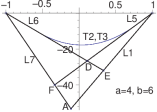
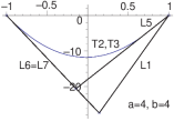
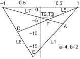
Figure 20: Bifurcation diagrams for Manakov top corresponding to fixed $a=4$ value and to $b=6,4,2$.

    

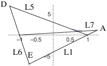
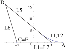
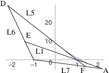
Figure 21: Bifurcation diagrams for Manakov top corresponding to fixed value of $a$ and to three different values of $b=0.5,0,-0.5$.

Some modifications of bifurcation diagram under the variation of $a,b$ parameters are shown in Fig. 20 and in Fig. 21.

Different limiting cases of the bifurcation diagram are represented in Figs. 22 and 23.

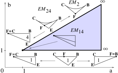
Figure 22: Limiting cases of bifurcation diagram ($a>b>1$). Small figures are the images of EM diagram for ‘critical’ values of $a$, $b$ parameters and the numbers show what regions of the image do not vanish in that limit. The capital letters indicate the position of zero rank critical values of EM map.

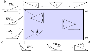
Figure 23: Limiting cases of EM diagram ($a>1$, $1>b>0$).

It is quite interesting to see the correspondence between images of EM maps for different limiting cases of Manakov top and EM diagrams for geodesic flow on three-dimensional ellipsoids with partially coinciding semi-axes [10, 11].

Acknowledgments

This work was stimulated by the initial discussions with Vadim Kuznetsov. Authors thank Dr. D. Sadovskii for many fruitful discussions and Dr. C. Davison for discussing with us his recent results submitted for publication [10, 11].

References

- [1]
- [2] Adler M., van Moerbeke P., The Kowalewski and Hénon–Heiles motions as Manakov geodesic flows on – a two-dimensional family of Lax pairs, Comm. Math. Phys. 113 (1988), 659–700.
- [3] Audin M., Spinning tops, Cambridge University Press, Cambridge, 1996, Chapter 4.
- [4] Bolsinov A.V., Fomenko A.T., Integrable Hamiltonian systems. Geometry, topology, classification, Chapman & Hall/CRC London, 2004, Section 14.
- [5] Cejnar P., Macek M., Heinze S., Jolie J., Dobes J., Monodromy and excited-state quantum phase transitions in integrable systems: collective vibrations of nuclei, J. Phys. A: Math. Gen. 39 (2006), L515–L521.
- [6] Child M.S., Quantum monodromy and molecular spectroscopy, Adv. Chem. Phys., to appear.
- [7] Colin de Verdière Y., Vũ Ngọc S., Singular Bohr–Sommerfeld rules for 2D integrable systems, Ann. Sci. Ècole Norm. Sup. (4) 36 (2003), 1–55, math.AP/0005264.
- [8] Cushman R.H., Bates L.M., Global aspects of classical integrable systems, Birkhäuser, Basel, 1997.
- [9] Cushman R.H., Sadovskii D., Monodromy in the hydrogen atom in crossed fields, Phys. D 142 (2000), 166–196.
- [10] Davison C.M., Dullin H.R., Bolsinov A.V., Geodesics on the ellipsoid and monodromy, math-ph/0609073.
- [11] Davison C.M., Dullin H.R., Geodesic flow on three dimensional ellipsoids with equal semi-axes, math-ph/0611060.
- [12] Duistermaat J.J., On global action angle coordinates, Comm. Pure Appl. Math. 33 (1980), 687–706.
- [13] Efstathiou K., Cushman R.H., Sadovskii D.A., Fractional monodromy in the resonance, Adv. Math. 209 (2007), 241–273.
- [14] Efstathiou K., Sadovskii D., Zhilinskii B., Analysis of rotation-vibration relative equilibria on the example of a tetrahedral four atom molecule, SIAM J. Appl. Dyn. Syst. 3 (2004), 261–351.
- [15] Grondin L., Sadovskii D., Zhilinskii B., Monodromy in systems with coupled angular momenta and rearrangement of bands in quantum spectra, Phys. Rev. A 65 (2002), 012105, 15 pages.
- [16] Kalnins E. G., Miller W.Jr., Winternitz P., The group , separation of variables and the hydrogen atom, SIAM J. Appl. Math. 30 (1976), 630–664.
- [17] Komarov I.V., Kuznetsov V.B., Quantum Euler–Manakov top on the 3-sphere , J. Phys. A: Math. Gen. 24 (1991), L737–L742.
- [18] Leung N.C., Symington M., Almost toric symplectic four-manifolds, math.SG/0312165.
- [19] Manakov S.V., Note on the integration of Euler’s equation of the dynamics of an dimensional rigid body, Funct. Anal. Appl. 11 (1976), 328–329.
- [20] Michel L., Points critique des fonctions invariantes sur une -varieté, C. R. Math. Acad. Sci. Paris 272 (1971), 433–436.
- [21] Michel L., Zhilinskii B.I., Symmetry, invariants, and topology. I. Basic tools, Phys. Rep. 341 (2001), 11–84.
- [22] Nek͡horoshev N.N., Action-angle variables and their generalizations, Tr. Mosk. Mat. Obs. 26 (1972), 180–198.
- [23] Nek͡horoshev N. N., Sadovskií D.A., Zhilinskií B.I., Fractional monodromy of resonant classical and quantum oscillators, C. R. Math. Acad. Sci. Paris 335 (2002), 985–988.
- [24] Nek͡horoshev N. N., Sadovskii D., Zhilinskii B., Fractional Hamiltonian monodromy, Ann. Henri Poincaré 7 (2006), 1099–1211.
- [25] Oshemkov A.A., Topology of isoenergy surfaces and bifurcation diagrams for integrable cases of rigid body dynamics on , Uspekhi Mat. Nauk 42 (1987), 199–200.
- [26] Perelomov A.M., Motion of four-dimensional rigid body around a fixed point: an elementary approach. I, math-ph/0502053.
- [27] Sadovskii D., Zhilinskii B., Group theoretical and topological analysis of localized vibration-rotation states, Phys. Rev. A 47 (1993), 2653–2671.
- [28] Sadovskii D., Zhilinskii B., Monodromy, diabolic points, and angular momentum coupling, Phys. Lett. A 256 (1999), 235–244.
- [29] Sadovskii D., Zhilinskii B., Quantum monodromy, its generalizations and molecular manifestations, Mol. Phys. 104 (2006), 2595–2615.
- [30] Sadovskii D., Zhilinskii B., Hamiltonian systems with detuned resonance. Manifestations of bidromy, Ann. Physics 322 (2007), 164–200.
- [31] Symington M., Four dimensions from two in symplectic topology, in Topology and Geometry of Manifolds (2001, Athens, GA), Proc. Symp. Pure Math., Vol. 71, AMS, Providence, RI, 2003, 153–208, math.SG/0210033.
- [32] Winnewisser M., Winnewisser B., Medvedev I., de Lucia F.C., Ross S.C., Bates L.M., The hidden kernel of molecular quasi-linearity: quantum monodromy, J. Mol. Structure 798 (2006), 1–26.
- [33] Vũ Ngọc S., Quantum monodromy in integrable systems, Comm. Math. Phys. 203 (1999), 465–479.
- [34] Vũ Ngọc S., Moment polytopes for symplectic manifolds with monodromy, Adv. Math. 208 (2007), 909–934, math.SG/0504165.
- [35] Zhilinskii B.I., Symmetry, invariants, and topology. II Symmetry, invariants, and topology in molecular models, Phys. Rep. 341 (2001), 85–171.
- [36] Zhilinskii B., Interpretation of quantum Hamiltonian monodromy in terms of lattice defects, Acta Appl. Math. 87 (2005), 281–307.
- [37] Zhilinskii B., Hamiltonian monodromy as lattice defect, in Topology in Condensed Matter, Editor M.I. Monastyrsky, Springer, Berlin, 2006, 165–186, quant-ph/0303181.