The spherically symmetric $\alpha^{2}-$dynamo and some of its spectral peculiarities

Abstract

A brief overview is given over recent results on the spectral properties of spherically symmetric MHD $\alpha^{2}-$dynamos. In particular, the spectra of sphere-confined fluid or plasma configurations with physically realistic boundary conditions (BCs) (surrounding vacuum) and with idealized BCs (super-conducting surrounding) are discussed. The subjects comprise third-order branch points of the spectrum, self-adjointness of the dynamo operator in a Krein space as well as the resonant unfolding of diabolical points. It is sketched how certain classes of dynamos with a strongly localized $\alpha-$profile embedded in a conducting surrounding can be mode decoupled by a diagonalization of the dynamo operator matrix. A mapping of the dynamo eigenvalue problem to that of a quantum mechanical Hamiltonian with energy dependent potential is used to obtain qualitative information about the spectral behavior. Links to supersymmetric Quantum Mechanics and to the Dirac equation are indicated.

Preliminaries
The magnetic fields of planets, stars and galaxies are maintained by dynamo effects in conducting fluids or plasmas [1, 2, 3]. These dynamo effects are caused by a topologically nontrivial interplay of fluid (plasma) motions and a balanced self-amplification of the magnetic fields — and can be described within the framework of magnetohydrodynamics (MHD) [1, 2].

For physically realistic dynamos the coupled system of Maxwell and Navier-Stokes equations has, in general, to be solved numerically. For a qualitative understanding of the occurring effects semi-analytically solvable toy models play an important role. One of the simplest dynamo models is the so called $\alpha^{2}-$dynamo with spherically symmetric $\alpha-$profile $\alpha(r)$ (see, e.g. [2]). For such a dynamo the magnetic fields can be decomposed in poloidal and toroidal components, expanded over spherical harmonics [2, 4] and unitarily re-scaled [5]. As result one arrives at a set of $l-$mode decoupled $2\times 2-$matrix differential eigenvalue problems [2, 4, 5]

$$\mathfrak{A}_{\alpha}=\left(\begin{array}[]{cc}-Q[1]&\alpha\\ Q[\alpha]&-Q[1]\end{array}\right),\qquad Q[\alpha]:=-\partial_{r}\alpha(r)\partial_{r}+\alpha(r)\frac{l(l+1)}{r^{2}}$$ (1)

with boundary conditions (BCs) which have to be imposed in dependence of the concrete physical setup and which will be discussed below. The $\alpha-$profile describes the net effect of small scale helical turbulence on the magnetic field [2]. It can be assumed real-valued $\alpha(r)\in\mathbb{R}$ and sufficiently smooth. We note that the reality of the differential expression (1), independently from the concrete BCs, implies an operator spectrum which is symmetric with regard to the real axis, i.e. which consists of purely real eigenvalues and of complex conjugate eigenvalue pairs.

In [4] it was shown that the differential expression (1) of this operator has the fundamental (canonical) symmetry [6, 7]

$$\mathfrak{A}_{\alpha}=J\mathfrak{A}_{\alpha}^{\dagger}J,\qquad J=\left(\begin{array}[]{cc}0&I\\ I&0\end{array}\right)\,.$$ (2)

In case of BCs compatible with this fundamental symmetry the operator turns out self-adjoint in a Krein space $(\mathcal{K}_{J},[.,.]_{J})$ [4, 5] and in this way it behaves similar like Hamiltonians of $\mathcal{P}\mathcal{T}-$symmetric Quantum Mechanics (PTSQM) [9, 10, 11, 12, 13, 14].

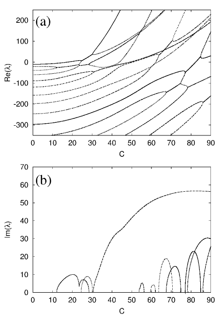
Figure 1: Real and imaginary components of the $\alpha^{2}-$dynamo spectrum as functions of the scale factor $C$ of an $\alpha-$profile $\alpha(r)=C\times(1-26.09\times r^{2}+53.64\times r^{3}-28.22\times r^{4})$ in the case of angular mode number $l=1$ and physically realistic boundary conditions (The spherically symmetric $\alpha^{2}-$dynamo and some of its spectral peculiarities). The concrete coefficients in the quartic polynomial $\alpha(r)$ have their origin in numerical simulations of field reversal dynamics (see Ref. [20, 21]). Only the imaginary components with $\Im\lambda\geq 0$ are shown. The symmetrically located complex conjugate $(\Im\lambda\leq 0)-$components are omitted for sake of brevity.

Subsequently, we first present a sketchy overview of some recent results on the spectral behavior of $\alpha^{2}-$dynamos obtained in [5, 15, 16, 17, 18, 19] which we extend by a discussion of the transition from $\alpha^{2}-$dynamo configurations confined in a box to dynamos living in an unconfined conducting surrounding.

Physically realistic BCs and spectral triple points
For roughly spherically symmetric dynamical systems like the Earth the conducting fluid is necessarily confined within the core of the Earth so that the $\alpha-$effect resulting from the fluid motion has to be confined to this core. Setting the surface of the outer core at a radius $r=1$ one can assume $\alpha(r>1)=0$ and a behavior of the magnetic field at $r>1$ like in vacuum. A multi-pole-like decay of the magnetic field at $r\to\infty$ leads then to mixed effective BCs at $r=1$ (see, e.g. [2]) and an corresponding operator domain of the type

$$\mathcal{D}(\mathfrak{A}_{\alpha})=\left\{\mathfrak{u}\in\tilde{\mathcal{H}}=L_{2}(0,1)\oplus L_{2}(0,1)|\ \mathfrak{u}(r\searrow 0)=0,\ \ \mathfrak{B}\mathfrak{u}|_{r\nearrow 1}=0\right\},$$

$$\mathfrak{u}:=\left(\begin{array}[]{c}u_{1}\\ u_{2}\\ \end{array}\right),\qquad\mathfrak{B}:=\left(\begin{array}[]{cc}\partial_{r}+\frac{l}{r}&0\\ 0&1\\ \end{array}\right).$$ (7)

From the domain $\mathcal{D}(\mathfrak{A}_{\alpha}^{\dagger})$ of the adjoint operator

$$\mathcal{D}(\mathfrak{A}_{\alpha}^{\dagger})=\left\{\hat{\mathfrak{u}}\in\hat{\mathcal{H}}=L_{2}(0,1)\oplus L_{2}(0,1)|\ \hat{\mathfrak{u}}(r\searrow 0)=0,\ \ \hat{\mathfrak{B}}\hat{\mathfrak{u}}|_{r\nearrow 1}=0\right\},$$

$$\hat{\mathfrak{u}}:=\left(\begin{array}[]{c}\hat{u}_{1}\\ \hat{u}_{2}\\ \end{array}\right),\qquad\hat{\mathfrak{B}}:=\left(\begin{array}[]{cc}\partial_{r}+\frac{l}{r}&-\alpha(r)\partial_{r}\\ 0&1\\ \end{array}\right)$$ (12)

one reads off that $\mathcal{D}(\mathfrak{A}_{\alpha}^{\dagger})\neq\mathcal{D}(\mathfrak{A}_{\alpha})$ and, hence, the dynamo operator $\mathfrak{A}_{\alpha}$ itself is not self-adjoint even in a Krein space.

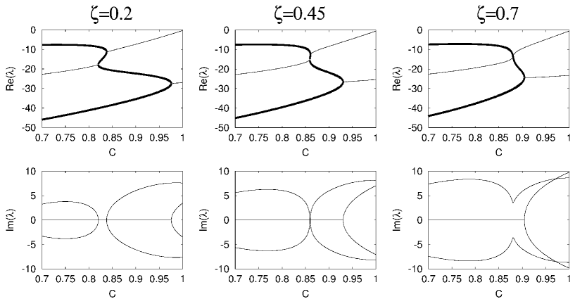
Figure 2: $\alpha^{2}-$dynamo with $\alpha(r)=C\left[-(21.465+2.467\zeta)+(426.412+167.928\zeta)r^{2}-(806.729+436.289\zeta)r^{3}\right.$ $\left.+(392.276+272.991\zeta)r^{4}\right]$ and a spectral triple point at $(\zeta=0.45,C=0.86)$. Highlighted (fat) lines correspond to purely real branches of the spectrum. The cusp in the imaginary component (lower right graphics) indicates the closely located triple point.

In case of constant $\alpha-$profiles and arbitrary $l\in\mathbb{N}$, the spectrum is implicitly given by a characteristic equation built from spherical Bessel functions [2]. In all other cases numerical studies are required. A typical spectral branch graph is depicted in Fig. 1. Obviously, for the specific $\alpha-$profile it contains a large number of spectral phase transitions from real spectral branches to complex ones and back. There are strong indications that phase transition points (second order branch points/exceptional points) of the spectrum close to the $\lambda=0$ line play an important role in polarity reversals of the magnetic field (see [20, 21, 22, 23] for numerical studies and [24] for recent experiments).

Apart from the second-order branch points visible in Fig. 1 there may occur third- and higher-order branch points. They are located on hyper-surfaces of higher co-dimension in parameter space and they therefore require a tuning of more parameters to pin them down. Corresponding results have been obtained in [16] and are illustrated in Fig. 2. The triple points result from coalescing second-order branch points, correspond to $3\times 3$ Jordan blocks in the spectral decomposition of the operator and are accompanied by a merging or disconnecting of two complex spectral sectors over the parameter space. An implicit indication of a closely located triple point is the presence of cusps in the imaginary components as they are visible in Figs. 1, 2.

Idealized BCs and Krein-space related perturbation theory
In order to gain some deeper insight into possible dynamo-related processes semi-analytical toy model considerations play a crucial role. A certain simplification of the eigenvalue problem has been achieved in [17, 18] by considering a reduced and idealized (auxiliary) problem with Dirichlet BCs imposed at $r=1$, i.e. by setting $\mathfrak{u}(r=1)=0$.

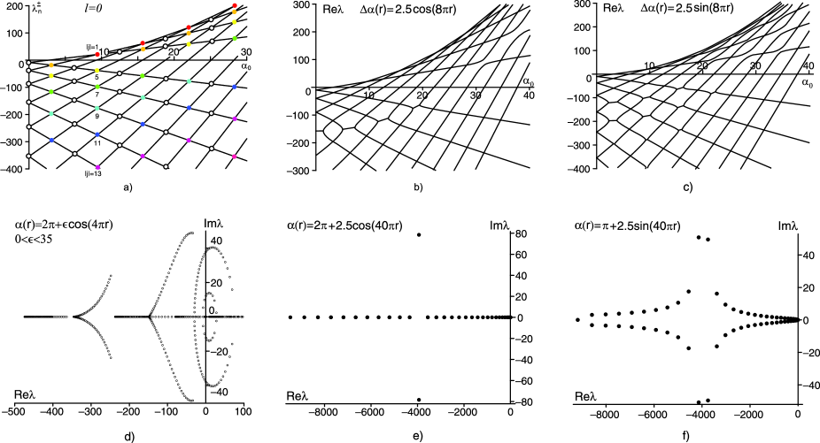
Figure 3: The spectral mesh of the operator matrix $\mathfrak{A}_{\alpha}$ for $l=0$ (a); its resonant deformation due to harmonic perturbations of a constant $\alpha$-profile (b), (c); the formation of overcritical oscillatory dynamo regimes for $\epsilon$ increasing from $\epsilon=0$ ($\Im\lambda=0$) to $\epsilon=35$ ($\Re\lambda>0$, $\Im\lambda\neq 0$ for some branches) (d); and the resonant unfolding of DPs in the complex plane (e), (f).

In this case it holds $\mathcal{D}(\mathfrak{A}_{\alpha})=\mathcal{D}(\mathfrak{A}_{\alpha}^{\dagger})$ and the operator $\mathfrak{A}_{\alpha}$ is self-adjoint in a Krein space $(\mathcal{K}_{J},[.,.]_{J})$ [5]. For constant $\alpha-$profiles $\alpha(r)=\alpha_{0}=\mbox{\rm const}\,$ the eigenvalue problem $(\mathfrak{A}_{\alpha_{0}}-\lambda)\mathfrak{u}=0$ becomes exactly solvable in terms of orthonomalized Riccati-Bessel functions

$$u_{n}(r)=N_{n}r^{1/2}J_{l+\frac{1}{2}}(\sqrt{\rho_{n}}r),\qquad N_{n}:=\frac{\sqrt{2}}{J_{l+\frac{3}{2}}(\sqrt{\rho_{n}})},\qquad(u_{m},u_{n})=\delta_{mn},\qquad\|u_{n}\|=1$$ (13)

with $\rho_{n}>0$ the squares of Bessel function roots $J_{l+\frac{1}{2}}(\sqrt{\rho_{n}})=0$. The solutions of the eigenvalue problem have the form

$$\mathfrak{u}_{n}^{\pm}=\left(\begin{array}[]{c}1\\ \pm\sqrt{\rho_{n}}\\ \end{array}\right)u_{n}\in\mathbb{R}^{2}\otimes L_{2}(0,1)\,,$$ (14)

are Krein space orthonormalized

$$[\mathfrak{u}_{m}^{\pm},\mathfrak{u}_{n}^{\pm}]=\pm 2\sqrt{\rho_{n}}\delta_{mn},\qquad[\mathfrak{u}_{m}^{\pm},\mathfrak{u}_{n}^{\mp}]=0,\qquad\mathfrak{u}_{n}^{\pm}\in\mathcal{K}_{\pm}\subset\mathcal{K},\qquad\mathfrak{u}_{n}^{\pm}=:\mathfrak{u}_{n}^{\varepsilon},\ \varepsilon=\pm$$ (15)

and correspond to eigenvalue branches $\lambda_{n}^{\varepsilon}=-\rho_{n}+\varepsilon\alpha_{0}\sqrt{\rho_{n}}$ which scale linearly with $\alpha_{0}$. In the $(\alpha_{0},\Re\lambda)-$plane the branches $\lambda_{n}^{+}$ and $\lambda_{n}^{-}$ of states $\mathfrak{u}^{+}_{n}$, $\mathfrak{u}_{n}^{-}$ of positive and negative Krein space type form a spectral mesh (see Fig. 3). The intersection points (nodes of the mesh) are semisimple double eigenvalues, i.e. eigenvalues of geometrical and algebraical multiplicity two — so called diabolical points (DPs) [26]. Two given branches $\lambda_{n}^{\varepsilon}(\alpha_{0})$ and $\lambda_{m}^{\delta}(\alpha_{0})$ intersect at the single point $\lambda=\lambda^{\nu}_{0}:=\varepsilon\delta\sqrt{\rho_{n}\rho_{m}}$,  $\alpha_{0}=\alpha_{0}^{\nu}:=\varepsilon\sqrt{\rho_{n}}+\delta\sqrt{\rho_{m}}$ and one obtains that branches from states of opposite Krein space type $\varepsilon=-\delta$ intersect for $\lambda_{0}^{\nu}<0$, whereas states of the same type $(\varepsilon=\delta)$ intersect at $\lambda_{0}^{\nu}>0$. Under small inhomogeneous perturbations $\alpha(r)=\alpha_{0}^{\nu}+\Delta\alpha(r)=\alpha_{0}^{\nu}+\epsilon\phi(r)$ the diabolical points split $\lambda_{0}^{\nu}\mapsto\lambda_{0}^{\nu}+\epsilon\lambda_{1}+\ldots$ into two real or complex points (see also [27] for similar considerations) with leading contribution $\lambda_{1}$ resulting from the quadratic equation

$$\lambda_{1}^{2}-\lambda_{1}\left(\varepsilon\frac{[\mathfrak{B}\mathfrak{u}_{n}^{\varepsilon},\mathfrak{u}_{n}^{\varepsilon}]}{2\sqrt{\rho_{n}}}+\delta\frac{[\mathfrak{B}\mathfrak{u}_{m}^{\delta},\mathfrak{u}_{m}^{\delta}]}{2\sqrt{\rho_{m}}}\right)+\varepsilon\delta\frac{[\mathfrak{B}\mathfrak{u}_{n}^{\varepsilon},\mathfrak{u}_{n}^{\varepsilon}][\mathfrak{B}\mathfrak{u}_{m}^{\delta},\mathfrak{u}_{m}^{\delta}]-[\mathfrak{B}\mathfrak{u}_{n}^{\varepsilon},\mathfrak{u}_{m}^{\delta}]^{2}}{4\sqrt{\rho_{n}\rho_{m}}}=0\,,$$ (16)

where

$$[\mathfrak{B}\mathfrak{u}_{m}^{\delta},\mathfrak{u}_{n}^{\varepsilon}]=\int_{0}^{1}\varphi\left[\left(\varepsilon\delta\sqrt{\rho_{n}\rho_{m}}+\frac{l(l+1)}{r^{2}}\right)u_{m}u_{n}+u_{m}^{\prime}u_{n}^{\prime}\right]dr.$$ (17)

The unfolding of the DPs follows the typical Krein space rule. When they result from branches of the same type $(\varepsilon=\delta,\lambda_{0}^{\nu}>0)$ then the corresponding DPs unfold purely real-valued, whereas DPs from branches of opposite type $(\varepsilon=-\delta,\lambda_{0}^{\nu}<0)$ may unfold into complex conjugate eigenvalue pairs. This behavior is clearly visible in Fig. 3 b,c. Direct inspection reveals that the spectral meshes of unperturbed operators $\mathfrak{A}_{\alpha_{0}}$ for $l=0$ and $0<l\ll\infty$ show strong qualitative similarities so that results obtained for the quasi-exactly solvable $(l=0)-$model will qualitatively hold for models with $0<l\ll\infty$ too. Via Fourier expansion of $\alpha(r)$ a very pronounced resonance has been found along parabolas in the $(\alpha_{0},\Re\lambda)-$plane indicated by white and colored dots in Fig. 3a — leaving regions away from these parabolas almost unaffected. An especially pronounced resonance is induced by cosine perturbations which in linear approximation affect only the single parabola $j=2k$, Fig. 3b,e. Sine perturbations act strongest on parabolas $|j|=2k\pm 1$ with decreasing effect on $|j|=2k\pm m$ for increasing $m$ (see Fig. 3c,f). Physically important is the fact that higher mode numbers $k$ (shorter wave lengths of the $\Delta\alpha(r)$ perturbations) affect more negative $\Re\lambda$. Due to a magnetic field behavior $\propto e^{\lambda t}$ this is the mathematical formulation of the physically plausible fact that small-scale perturbations decay faster than large-scale perturbations. Numerical indications for the importance of this behavior in the subtle interplay of polarity reversals and so called excursions (”aborted” reversals) of the magnetic field have been recently given in [23].

Diagonalizable $\alpha^{2}-$dynamo operators, SUSYQM and the Dirac equation
Another approach to obtain quasi-exact solution classes of the eigenvalue problem $(\mathfrak{A}_{\alpha}-\lambda)\mathfrak{u}=0$ consists in a $\lambda-$dependent diagonalization of the operator matrix (1). The basic feature of this technique, as demonstrated in [19], is a two-step procedure consisting of a gauge transformation which diagonalizes the kinetic term and a subsequent global (coordinate-independent) diagonalization of the potential term. Such an operator diagonalization is possible for $\alpha-$profiles satisfying the constraint

$$\alpha^{\prime\prime}(r)+\frac{1}{2}\alpha^{3}(r)-a^{2}\alpha(r)=0$$ (18)

with $a=\mbox{\rm const}\,\in\mathbb{R}$ a free parameter. Solutions $\alpha(r)$ of this autonomous differential equation (DE) can be expressed in terms of elliptic integrals. In order to maximally explore similarities to known QM type models a strongly localized $\alpha-$profile has been assumed which smoothly vanishes toward $r\to\infty$. Physically, such a setup can be imagined as a strongly localized dynamo-maintaining turbulent fluid/plasma motion embedded in an unbounded conducting surrounding (plasma) with fixed homogeneous conductivity. The only $\alpha-$profile with $\alpha(r\to\infty)\to 0$ satisfying (18) has the form of a Korteweg-de Vries(KdV)-type one-soliton potential

$$\alpha(r)=\frac{2a}{\cosh[a(r-r_{0})]}\,.$$ (19)

This amazing finding indicates on deep structural links to KdV and supersymmetric quantum mechanics (SUSYQM) and opens up a completely new exploration approach to $\alpha^{2}-$dynamos. In [19] we restricted the consideration to the most elementary solution properties of such models. The decoupled equation set after a parameter and coordinate rescaling has been found in terms of two quadratic pencils

$$[-\partial_{x}^{2}+\frac{l(l+1)}{x^{2}}-\frac{1}{2}\alpha^{2}+\frac{1}{2}\mp\epsilon\alpha-\epsilon^{2}]F_{\pm}=0\,,\quad\alpha=\frac{2}{\cosh(x-x_{0})}$$ (20)

in the new variable $x:=ar$ and with new auxiliary spectral parameter $\epsilon=\left(\frac{1}{2}-\lambda\right)^{1/2}$. The equivalence transformation from $(\mathfrak{A}_{\alpha}-\lambda)\mathfrak{u}=0$ to (20) is regular for $\epsilon\neq 0$ and becomes singular at $\epsilon=0$ where (20) has to be replaced by a Jordan type equation system

$$\left(\begin{array}[]{cc}\partial_{x}^{2}-V_{0}&-V_{1}\\ 0&\partial_{x}^{2}-V_{0}\\ \end{array}\right)\left(\begin{array}[]{c}\Xi_{1}\\ \Xi_{0}\\ \end{array}\right)=0$$ (21)

with potentials $V_{0}=l(l+1)x^{-2}-\frac{1}{2}(\alpha^{2}-1)$, $V_{1}=-\alpha$. In terms of the original spectral parameter $\lambda$ the eigenvalue problems (20) read

$$\left[-\partial_{x}^{2}+\frac{l(l+1)}{x^{2}}-\frac{1}{2}\alpha^{2}\mp\left(\frac{1}{2}-\lambda\right)^{1/2}\alpha\right]F_{\pm}=-\lambda F_{\pm}$$ (22)

and can be related to the spectral problem of a QM Hamiltonian with energy $E=-\lambda$ and energy-dependent potential component $\mp\left(\frac{1}{2}-\lambda\right)^{1/2}\alpha(x)=\mp\left(E+\frac{1}{2}\right)^{1/2}\alpha(x)$. For physical reasons asymptotically vanishing field configurations with $F_{\pm}(x\to\infty)\to 0$, $\Xi_{0,1}(x\to\infty)\to 0$ are of interest. These Dirichlet BCs at infinity imply the self-adjointness of the operator $\mathfrak{A}_{\alpha}$ in a Krein space $\mathcal{K}_{J}$ — with (20), (21) as special representation of the eigenvalue problem $(\mathfrak{A}_{\alpha}-\lambda)\mathfrak{u}=0$. From the structure of (20),(22) follows that the only free parameter apart from the angular mode number $l\in\mathbb{N}$ is the maximum position $x_{0}$ of the $\alpha-$profile $\alpha(x)$ (the minimum position of the potential component $-\alpha^{2}(x)/2$) so that solution branches will be functions $\lambda(x_{0})$.

Figure 4: Spectra $\epsilon(x_{0})$ (a) and $\lambda(x_{0})$ (b) in case of angular mode numbers $l=0,1,2,3$. For numerical reasons the Dirichlet BC has been imposed at the large distance $x=100$.

With the help of SUSY techniques it has been shown in [19] that (22) has a single bound state (BS) type solution which via $E=-\lambda<0$ corresponds to an overcritical dynamo mode $\lambda>0$. It has been found that the BS solutions of (22) behave differently for $x_{0}<x_{J}$ and $x_{0}>x_{J}$, where for $x_{0}=x_{J}$ the description in terms of (20) breaks down and has to be replaced by the singular Jordan type representation (21). By a SUSY inspired factorization ansatz

$$-\partial_{x}^{2}+\frac{l(l+1)}{x^{2}}-\frac{1}{2}\alpha^{2}+\frac{1}{2}=L^{\dagger}L\,,$$ (23)

$$L=-\partial_{x}+w,\quad L^{\dagger}=\partial_{x}+w,\quad w=u^{\prime}/u\,,$$ (24)

an equivalence relation between (20) and a system of two Dirac equations

$$H_{\pm}\Psi_{\pm}=\epsilon\Psi_{\pm}\,,\quad H_{\pm}=\gamma\partial_{x}+V_{\pm}$$ (25)

$$\Psi_{\pm}=\left(\begin{array}[]{c}\psi_{1,\pm}\\ \psi_{2,\pm}\end{array}\right):=\left(\begin{array}[]{c}F_{\pm}\\ \epsilon^{-1}LF_{\pm}\end{array}\right),\quad\gamma=\left(\begin{array}[]{cc}0&1\\ -1&0\end{array}\right),\quad V_{\pm}=\left(\begin{array}[]{cc}\mp\alpha&w\\ w&0\end{array}\right)$$ (26)

has been established for models with $x_{0}<x_{J}$. General results on Dirac equations allowed then for the conclusion that in case of $x_{0}<x_{J}$ the bound state related spectrum has to be real. A perturbation theory with the distance $\delta=x_{0}-x_{J}$ from the Jordan configuration as small parameter supplemented by a bootstrap analysis showed that the Dirichlet BCs $F_{\pm}(x\to\infty)\to 0$ render only the solution $F_{+}(x)$ non-trivial and with real eigenvalue, whereas $F_{-}(x)$ has to vanish identically $F_{-}(x)\equiv 0$. The single spectral branch in terms of $\lambda(x_{0})$ and $\epsilon(x_{0})$ is depicted in Fig. 4 for angular mode numbers $l=0,1,2,3$.

Assuming the dynamo model with strongly localized $\alpha-$profile (19), (20) confined in a large box, i.e. with Dirichlet BCs imposed at large $x=X\gg 0$, one can study the dynamo spectrum in the infinite box limit.

Figure 5: Cutoff ($X$-)dependence of the spectral branches with radial mode numbers $n=1,2$ and angular mode numbers $l=0$ (a) and $l=2$ (b) for cutoffs (box-lengths) $X=10,\,20,\,40$. Clearly visible are the $X-$independence of the overcritical BS type modes $(n=1)$ and the tendency $\lambda\propto-1/X^{2}$ for the undercritical (box-type) mode. The modes with $n\geq 3$ show the same qualitative $\lambda\propto-1/X^{2}$ behavior like the $n=2$ mode and are note depicted here.

Figures 5 a,b show the corresponding behavior. Due to its localization the BS-related overcritical dynamo mode is almost insensitive to the $X\to\infty$ limit. This is in contrast to the under-critical (decaying) modes which behave as expected for a sign inverted box spectrum of QM. For fixed mode number $n\geq 2$ and $X\to\infty$ the energies $E_{n}$ decrease like $E_{n}\propto 1/X^{2}\searrow 0$ and the corresponding part of the spectrum becomes quasi-continuous and related to the continuous (essential) spectrum of QM scattering states of a particle moving in the energy dependent potential $\frac{l(l+1)}{x^{2}}-\frac{1}{2}\alpha^{2}(x)\mp\left(E+\frac{1}{2}\right)^{1/2}\alpha(x)$. For the associated dynamo eigenvalues this implies $\lambda_{n}\propto-1/X^{2}\nearrow 0$ — as it is clearly visible in Figures 5 a,b.

Concluding remarks
A brief overview over some recent results on the spectra of dynamo operators has been given. The obtained structural features like the resonance effects in the unfolding of diabolical points as well as the unexpected link to KdV soliton potentials, elliptic integrals, SUSYQM and the Dirac equation appear capable to open new semi-analytical approaches to the study of $\alpha^{2}-$dynamos.

Acknowledgement
The work reviewed here has been supported by the German Research Foundation DFG, grant GE 682/12-3 (U.G.), by the CRDF-BRHE program and the Alexander von Humboldt Foundation (O.N.K.) as well as by RFBR-06-02-16719 and SS-5103.2006.2 (B.F.S.).

References

- [1] H. K. Moffatt, Magnetic field generation in electrically conducting fluids, (Cambridge University Press, Cambridge, 1978).
- [2] F. Krause and K.-H. Rädler, Mean-field magnetohydrodynamics and dynamo theory, (Akademie-Verlag, Berlin and Pergamon Press, Oxford, 1980), chapter 14.
- [3] Ya. B. Zeldovich, A. A. Ruzmaikin and D. D. Sokoloff, Magnetic fields in astrophysics, (Gordon & Breach Science Publishers, New York, 1983).
- [4] U. Günther and F. Stefani, J. Math. Phys. 44, (2003), 3097, math-ph/0208012.
- [5] U. Günther, F. Stefani and M. Znojil, J. Math. Phys. 46, (2005), 063504, math-ph/0501069.
- [6] T. Ya. Azizov and I. S. Iokhvidov, Linear operators in spaces with an indefinite metric, (Wiley-Interscience, New York, 1989).
- [7] A. Dijksma and H. Langer, Operator theory and ordinary differential operators, in A. Böttcher (ed.) et al., Lectures on operator theory and its applications, (Fields Institute Monographs, Vol. 3, p. 75, Am. Math. Soc., Providence, RI, 1996).
- [8] J. Bognár, Indefinite inner product spaces, (Springer, New-York, 1974).
- [9] C. M. Bender and S. Boettcher, Phys. Rev. Lett. 24, 5243 (1998), physics/9712001.
- [10] C. M. Bender, S. Boettcher and P. N. Meisinger, J. Math. Phys. 40, 2201 (1999), quant-ph/9809072.
- [11] M. Znojil, Phys. Lett. A259, 220 (1999), quant-ph/9905020; M. Znojil, J. Phys. A 33 4203 (2000), math-ph/0002036; M. Znojil, F. Cannata, B. Bagchi, and R. Roychoudhury, Phys. Lett. B483, 284 (2000), hep-th/0003277.
- [12] A. Mostafazadeh, J. Math. Phys. 43, 205 (2002), math-ph/0107001; ibid. 43, 2814 (2002), math-ph/0110016; ibid. 43, 3944 (2002), math-ph/0203005.
- [13] C. M. Bender, D. C. Brody and H. F. Jones, Phys. Rev. Lett. 89, 270401 (2002), quant-ph/0208076.
- [14] C. M. Bender, ”Making sense of non-Hermitian Hamiltonians”, hep-th/0703096.
- [15] U. Günther, F. Stefani and G. Gerbeth, Czech. J. Phys. 54, (2004), 1075-1090, math-ph/0407015.
- [16] U. Günther and F. Stefani, Czech. J. Phys. 55, (2005), 1099-1106, math-ph/0506021.
- [17] U. Günther and O. N. Kirillov, J. Phys. A: Math. Gen. 39, (2006) 10057, math-ph/0602013.
- [18] O. N. Kirillov and U. Günther, Proc. Appl. Math. Mech. (PAMM) 6, (2006), 637-638.
- [19] U. Günther, B. F. Samsonov and F. Stefani, J. Phys. A: Math. Theor. 40, (2007), F169-F176, math-ph/0611036.
- [20] F. Stefani and G. Gerbeth, Phys. Rev. Lett. 94, (2005), 184506, physics/0411050.
- [21] F. Stefani, G. Gerbeth, U. Günther, and M. Xu, Earth Planet. Sci. Lett. 243, (2006), 828-840, physics/0509118.
- [22] F. Stefani, G. Gerbeth, U. Günther, Magnetohydrodynamics 42, (2006), 123-130; physics/0601011.
- [23] F. Stefani, M. Xu, L. Sorriso-Valvo, G. Gerbeth, U. Günther, ”Reversals in nature and the nature of reversals”, physics/0701026.
- [24] M. Berhanu et al , Eur. Phys. Lett. 77, (2007), 59001, physics/0701076.
- [25] M. Znojil, ”A return to observability near exceptional points in a schematic symmetric model”, Phys. Lett. B, to appear, quant-ph/0701232.
- [26] M. V. Berry and M. Wilkinson, Proc. R. Soc. Lond. A392, (1984), 15.
- [27] O. N. Kirillov and A. P. Seyranian, SIAM Journal on Applied Mathematics 64, (2004), 1383-1407.
- [28] R. Meinel, Astron. Nachr. 310, (1989), 1.
- [29] C. M. Bender, D. C. Brody, J. Chen, E. Furlan, J. Phys. A: Math. Theor. 40, (2007), F153-F160, math-ph/0610003.
- [30] A. Fring, ”symmetric deformations of the Korteweg-de Vries equation”, math-ph/0701036.