Spectral Curves of Operators with Elliptic Coefficients

Spectral Curves of Operators
with Elliptic Coefficients

J. Chris EILBECK ^†, Victor Z. ENOLSKI ^‡ and Emma PREVIATO ^§

J.C. Eilbeck, V.Z. Enolski and E. Previato

^† The Maxwell Institute and Department of Mathematics, Heriot-Watt University,
  Edinburgh, UK EH14 4AS J.C.Eilbeck@hw.ac.uk

^‡ Institute of Magnetism, 36 Vernadski Str., Kyiv-142, Ukraine

vze@ma.hw.ac.uk

^§ Department of Mathematics and Statistics, Boston University, Boston MA 02215-2411, USA ep@bu.edu

Received November 21, 2006, in final form February 16, 2007; Published online March 12, 2007

A computer-algebra aided method is carried out, for determining geometric objects associated to differential operators that satisfy the elliptic ansatz. This results in examples of Lamé curves with double reduction and in the explicit reduction of the theta function of a Halphen curve.

(equianharmonic) elliptic integrals; Lamé, Hermite, Halphen equation; theta function

33E05; 34L10; 14H42; 14H45

Dedicated to the memory of Vadim Kuznetsov

1 Introduction

The classical theory of reduction, initiated by Weierstrass, has found modern applications to the fields of Integrable Systems and Number Theory, to name but two. In this short note we only address specific cases, providing minimal historical references, listing the steps that we devised, and exhibiting some new explicit formulas. A full-length discussion of original motivation, theoretical advancements and modern applications would take more than one book to present fairly, and again, we choose to provide one (two-part) reference only, which is recent and captures our point of view [4, 5].

Our point of departure is rooted in the classical theory of Ordinary Differential Equations (ODEs). At a time when activity in the study of elliptic functions was most intense, Halphen, Hermite and Lamé (among many others) obtained deep results in the spectral theory of linear differential operators with elliptic coefficients. Using differential algebra, Burchnall and Chaundy described the spectrum (by which we mean the joint spectrum of the commuting operators) of those operators that are now called algebro-geometric, and some non-linear Partial Differential Equations (PDEs) satisfied by their coefficients under isospectral deformations along ‘time’ flows, $t_{1},\ldots,t_{g}$, where $g$ is the genus of the spectral ring. We seek algorithms that, starting with an Ordinary Differential Operator (ODO) with elliptic coefficients, produce an algebraic equation for an affine plane model of the spectral curve (Section 2). This problem turns out to merge with Weierstrass’ question [17], Appendix C:

Give a condition that an algebraic function $f(x)$ must satisfy if among the integrals

$$\int F(x,f(x))dx,$$

where $F$ is a rational function of $x$ and $f(x)$, there exist some that can be transformed into elliptic integrals.

This means that the curve $X$ whose function field is ${\mathbb{C}}(x,f(x))$ has a holomorphic differential which is elliptic, or equivalently, Jac $X$ contains an elliptic curve. Weierstrass gave a condition in terms of the period matrix of $X$. Burchnall–Chaundy spectral curves of operators with elliptic coefficients automatically come with this reduction property, because the differential-algebra theory guarantees that all the coefficients of the spectral ring are doubly-periodic with respect to the same lattice; the PDEs mentioned above have solutions which are called ‘elliptic solitons’. A more special condition is that there be a ‘multiple’ reduction, namely another periodicity with respect to a (possibly non-isomorphic) lattice, in which case a curve of genus three has Jacobian isogenous to the product of three elliptic curves, and this is what we found in [10]. Another difficult question is whether the Jacobian is actually complex-isomorphic (without the principal polarization, since Jacobians are indecomposable) to the product of three elliptic curves. This is the case for the Klein curve [3]; we do not know if it is for the Halphen curve in [10]. In genus two, the situation is only apparently simpler: the question of complex-isomorphism to a product has only recently been settled [7], and that, in an analytic but not in an algebraic language; the question of loci of genus-2 curves which cover ($n:1$) an elliptic curve remains largely open (despite recent progress, much of it based on computer algebra [30]).

In Section 3 of this paper, we provide progress towards such questions for the case of Lamé curves, which are hyperelliptic: the curves are known, at least for small genus, but we report a double reduction (equianharmonic case) that we have not seen elsewhere; in Section 4, we treat the genus 3 non-hyperelliptic case. Our contribution to a method consists of two parts. First, we provide algebraic maps between the higher-genus and the genus-one curves, by giving a search algorithm that identifies genus-1 integrals, the very question posed by Weierstrass. Second, using classical reduction theory as revisited by Martens [20], we write the theta function for a case of reduction in terms of genus-1 theta functions (or the associate sigma functions). We connect the two issues, by calculating explicitly the period matrix for some curve that admits reduction, given algebraically. It is a rare event, that a period matrix can be calculated from an algebraic equation, since the two in general are transcendental functions of each other. The method consists in the traditional one [3, 27, 28] of choosing a suitable homology basis and calculating the covering action on it. We believe our result on the period matrix of the Halphen curve and its reduction to be new. We also address the question of effectivization of the solution of the KP equation, or hierarchy; for this to be complete, however, we need not only to reduce the theta function, but also the integrals of differentials of the second kind.

We dedicate this small note to the memory of Vadim Kuznetsov. It was one of Vadim’s many projects to find a systematic answer to the problem of giving a canonical form for differential equations that have a basis of solutions polynomial in elliptic functions, generalizing the theory of elliptical harmonics given in the last chapter of [37], and which we have implemented in Section 3, to study the Lamé curves. In fact, one among us (VZE) co-authored one of the last papers of Vadim [38], devoted to a problem that arises in physics and was first identified by him; some of the ideas that we describe below were to be used in the further development of that subject. The loss of Vadim as friend and mathematician has affected us deeply. Personal memories and testimonials are collected in other parts of this issue; here we only say that it was our great privilege to know him.

2 Elliptic covers

Curves that admit a finite-to-one map to an elliptic curve (‘Elliptic Covers’) are special, and are a topic of extensive study in algebraic geometry and number theory. They have come to the fore in the theory of integrable equations, in particular their algebro-geometric solutions, for the reason that a yet more special class of such curves provides solutions that are doubly-periodic in one variable (‘Elliptic Solitons’).

Our point of view on the latter class of curves is based on the Burchnall–Chaundy theory, via which, we connect the problem to the theory of ODOs with elliptic coefficients, much studied in the nineteenth century (Lamé, Hermite, Halphen, e.g.). It is only when such an operator has a large commutator that this theory connects with that of integrable equations. While the nineteenth-century point of view could not have phrased the special property in this way, the related question that was addressed was, when does the series expansion of solutions, in some suitable local coordinate on the curve (cf. Remark 1 in Subsection 3.1) terminate? The early work turned up important, but somehow ad hoc, properties that characterize algebro-geometric operators.

2.1 Challenge I

Detect (larger) classes of algebro-geometric operators.

We do not address this issue here. A CAS-based project would be to test whether the operator

$$L=\partial^{3}-\dfrac{4}{3}n^{2}\wp\partial+\dfrac{2n(n-3)(4n+3)}{27}\wp^{\prime}$$

has centralizer larger than ${\mathbb{C}}[L]$: we ask the question since Halphen [15] noticed that the equation $L=0$ has solutions that can be expressed in terms of elliptic functions. A more far-reaching project would construct elliptic-coefficient, finite-gap operators starting with curves that were shown to be elliptic covers, choosing a local coordinate whose suitable power is a function pulled back from the elliptic curve, to give rise to the commutative ring of ODOs, according to the Burchnall–Chaundy–Krichever inverse spectral theory. Curves of genus 3 that are known to be elliptic $3:1$ and $2:1$ covers, respectively, are Klein’s and Kowalevski’s quartic curves:

$$zx^{3}+xy^{3}+yz^{3}=0,$$

$$(z^{2}-f_{2})^{2}=4xy(ax+by)(cx+dy)$$

in projective coordinates, with $f_{2}$ a form of degree 2 in $x$ and $y$ (such that the quartic is non-singular). Notably, Klein’s curve (the only curve of genus 3 that has maximum number of automorphisms, 168) has Jacobian which is isomorphic to the product of three (isomorphic) elliptic curves [3, 24, 26]; Kowalevski, as part of her thesis, classified the (non-hyperelliptic) curves of genus 3 that cover $2:1$ an elliptic curve (Klein’s curve being a special case).

2.2 Challenge II

Find an equation for the spectral curve.

This can be found once an algebro-geometric ODO is given. While the Burchnall–Chaundy theory allows one in principle to write the equation of the curve as a differential resultant [25], this would be unwieldy for all but the simplest cases: first, one would have to solve the ODEs of commutation $[L,B]=0$ for an unknown operator $B$ of order co-prime with $L$ (the simplest case of a two-generator centralizer); then, once $B$ is known, calculate the determinant of the $(m+n)\times(m+n)$ matrix that detects the common eigenfunctions of $L-\lambda$ and $B-\mu$ [9].

Instead, it is much more efficient to adapt Hermite’s (or Halphen’s) ansatz; in the case of Lamé’s equation, the case of solutions ‘written in finite form’ is treated in [37]; more generally, assume that an eigenfunction can be written in terms of:

$$\Psi(x;\alpha)=e^{kx}\sum_{j=0}^{n-1}a_{j}(x,\mu,k)\dfrac{d^{j}}{dx^{j}}\Phi(x;\alpha)$$

solving a given spectral problem: $L\Psi(x)=z\Psi(x)$, where:

$$\Phi(x,\alpha)=-\dfrac{\sigma(x-\alpha)}{\sigma(\alpha)\sigma(x)}e^{\zeta(\alpha)x}$$

and $\alpha$ is a complex number viewed as a point of the elliptic curve $\nu^{2}=4\mu^{3}-g_{2}\mu-g_{3}$.

By expanding $\wp(x)$ and $\phi(x,\alpha)$ near $x=0$ and comparing coefficients, the $a_{j}$ can be written in terms of ($k,z$) and taking the resultant of the compatibility conditions gives an equation of the spectral curve in the ($k,z$)-plane [8].

2.3 Challenge III

Express the eigenfunctions in terms of the theta function of the curve.

2.4 Challenge IV

Turn on the KP (isospectral-)time deformations $t_{i}$ and express the time-dependence of the coefficients of the operators (in particular, one such coefficient is an exact solution of the KP equation). The expression of a KP solution in terms of elliptic functions is part of the programme sometimes referred to as ‘effectivization’.

Our approach to such ‘challenges’ is two-fold: on one hand we use the explicit expression of the higher-genus sigma functions that were classically proposed by Klein and Baker, but revived, substantively generalized, and brought into usable form at first by one of the authors with collaborators (cf. e.g. [6]). On the other hand, we design computer algebra routines which allow us to read, for example, coefficients of multi-variable Taylor expansions far enough to obtain the equations for the curves and the KP solutions for small genus.

In this paper we present classes of examples, originating with classical ansatzes of Lamé, Hermite and Halphen (specifically applied to elliptic solitons by Krichever [18]) as well as some detail of our general strategy.

3 Hyperelliptic case

The Lamé equation has been vastly applied and vastly studied: we refer to [19] for general information, and to the classical treatise [37] for calculations that we shall need (for richer sources please consult [12], and [13] for different perspectives). Our point of view is that the potentials $n(n+1)\wp(\xi)$ are finite-gap when $n$ is an integer (an adaptation of Ince’s theorem to the complex-valued case) where the equation is written in Weierstrass form:

$$\dfrac{d^{2}w(\xi)}{d\xi^{2}}-n(n+1)\wp(\xi)w(\xi)=zw(\xi)$$ (1)

(for the rational form see [19] or [37]).

3.1 The spectral curve

The Lamé curves are hyperelliptic since one of the commuting differential operators has order 2, and will have genus $n$ for the operator in (1). There is no ‘closed form’ for general $n$, but the equations have been found by several authors and methods, cf. specifically [4, 5] and references therein (work by Eilbeck et al., by Enol’skii and N.A. Kostov, by A. Treibich and by J.-L. Verdier is there referenced), [14, 19, 22, 35]. In particular, [19] adopts a method of inserting ansatzes in the equation and comparing expansions similar to ours, and tabulates the equations for $1\leq g\leq 8$ (in principle, a recursive calculation will produce them for any genus), so we do not present our table ($1\leq g\leq 10$), but use $g=3$ to exemplify our treatment of reduction in Subsection 3.2 below.

Remark 3.1.

To motivate the project that Vadim Kuznetsov had wanted to design, as recalled in the introduction, we mention in sketch the steps of our strategy to find the spectral curves. The key ansatz is the finite expansion of the eigenfunctions; we used a formula from [37] in the case of odd $n$ and the (equivalent) table in [2] for even $n$ just for bookkeeping purposes; respectively,

$$w(\xi)=\sqrt{\wp(\xi)-e_{{1}}}\sqrt{\wp(\xi)-e_{2}}\sum_{r=0}^{(n-3)/2}b_{{r}}(\wp(\xi)-e_{3})^{n/2-r-1},\qquad w(\xi)=\sum_{r=0}^{n/2}A_{{r}}(-\wp(\xi))^{r}.$$

It is then a matter of finding the coefficients $b_{r},\ A_{r}$. For this, we insert $w$ in (1) and expand in powers of $\wp(\xi)$ or $(\wp(\xi)-e_{i})^{1/2}$, depending on the various cases; we also substitute for the $e_{i}$ in terms of the modular functions $g_{2}$ and $g_{3}$. By comparing coefficients in the expansions we obtain a set of equations for the $b_{r}$ or $A_{r}$, and we solve the compatibility condition of these equations. The Lamé curve $f_{s}(z)\prod\limits_{i=1}^{3}f_{i}(z)$ is the product of 4 factors, one $f_{s}(z)$ symmetric in the $e_{i}$, i.e. just depending on $g_{2}$ and $g_{3}$, and three $f_{i}(z)$ which depend on one of the $e_{i}$ and $g_{2}$ and $g_{3}$, which we found in turn. At the end, to be sure, for a given root $z$ of one of these factors, we can determine the $b_{r}$, resp. $A_{r}$ up to a common factor, and write the eigenfunction as a polynomial in $\wp(\xi)$. The finiteness condition we used in expanding the eigenfunctions (a sort of Halphen’s ansatz, cf. Section 1) characterizes finite-gap operators, in Burchnall–Chaundy terms, the ones that have large centralizers. It is worth quoting a speculation [29] p. 34 which regards finiteness in the local parameter $z^{-1}$: ‘We do not know an altogether satisfying description of the desired class ${\cal C}^{(n)}$; roughly speaking, it consists of the operators whose formal Baker functions converge for large $z$.’

3.2 Cover equations and reduction

Even though the Lamé curves are elliptic covers a priori, it is not easy to find the elliptic reduction, which will correspond to a holomorphic differential of smallest order at the point $\infty$ in $(w,z)$-coordinates; by running through a linear-algebra elimination for a basis of holomorphic differentials, expressed in terms of rational functions of $(w,z)$ (here again expansions provide the initial guess, lest the programs exhaust computational power), we exhibited the elliptic differential for all our curves. Note that this gives the degree of the cover, not known a priori. It is worth pointing out that more than $n$ covers might be found (for genus $n$): indeed, according to a classical result (Bolza, Poincaré, cf. [16] where a modern proof is given), if an abelian surface contains more than one elliptic subgroup, then it contains infinitely many. Note, however, that it can only contain a finite number for any given degree (the intersection number with a principal polarization) because the Néron–Severi group is finitely generated [16]. This degree translates into the degree of the elliptic cover. We are not claiming to have found all of them, or that those which we found be minimal. For example, for genus $n=2$ (where the reduction is known since the nineteenth century), finding $f_{s}=z^{2}-3g_{2}$, $f_{i}=z+3e_{i}$, in expanded form the curve is:

$${w}^{2}=-(3g_{2}-{z}^{2})(27g_{3}-4{z}^{3}+9zg_{2}).$$

The holomorphic differential is

$$\dfrac{d\wp}{\wp^{\prime}}=3z\dfrac{dz}{w},$$

and a second reduction (predicted by a classical theorem of Picard that splits any abelian subvariety up to isogeny) is given by the algebraic map to:

$${\wp^{\prime}}^{2}=4{\wp}^{3}-G_{2}\wp-G_{3},\qquad G_{2}=\frac{27}{4}(g_{2}^{3}+9g_{3}^{2}),\qquad G_{3}=\frac{243}{8}g_{3}(3g_{3}^{2}-g_{2}^{3}),$$

$$\wp=-\frac{1}{4}\,(4z^{3}-9g_{2}z-9g_{3}),\qquad\wp^{\prime}=-\frac{1}{2}\,w\,(4z^{2}-3g_{2}).$$

This map induces the following reduction of the holomorphic differential to an elliptic differential:

$$\frac{d\wp}{\wp^{\prime}}=-3\frac{d}{w}.$$

Notice then that in the equianharmonic case $g_{2}=0$ the curve is singular, $w^{2}=-(4z^{3}-27g_{3})z^{2}$ and we have the following birational map to the elliptic curve:

$${\wp^{\prime}}^{2}=4{\wp}^{3}-G_{3},\qquad\wp=-\frac{z}{4},\qquad\wp^{\prime}=\frac{-2w}{4z},\qquad G_{3}=-\frac{27}{64}g_{3}$$

and differential $d\wp/\wp^{\prime}=zdz/2w.$ This motivated us to investigate the equianharmonic case further.

What we believe to be new is the following observation. We found it surprising that there always be at least a second reduction in the case the elliptic curve is equianharmonic (the unique one that has an automorphism of order three), but see no theoretical reason to expect that. If this were to hold for all $n$, one could further ask whether these curves support KdV solutions elliptic both in the first and second time variables (a private communication by A. Veselov gives such an indication, to the best of our understanding). The issue of periodicity in the second KdV variable (‘time’) was put forth in [31], and recently reprised in [11], but the double periodicity does not seem to have been addressed so far. We exhibit three covers in the $g=3$ case (N.B. The third one is not, in general, over the equianharmonic curve); as well, we found two covers in the equianharmonic, $n=4,5$ cases, but we only provide a summary table which suggests the general pattern for two covers in the equianharmonic case.

For $n=3$, $f_{s}=z$, $f_{i}=z^{2}-6ze_{i}+45e_{i}^{2}-15g_{2}$, the curve is

$${w}^{2}=\big{(}2376\,{z}^{3}g_{3}-36450\,zg_{2}g_{3}+504\,g_{{2}}{z}^{4}-91125\,{g_{3}}^{2}-16\,{z}^{6}+3375\,{g_{2}}^{3}-4185\,{g_{2}}^{2}{z}^{2}\big{)}z,$$

the first cover is given by the algebraic map

$$\wp=-\frac{(-84375g_{2}^{3}+2278125g_{3}^{2}+303750g_{3}g_{2}z-3375g_{2}^{2}z^{2}-27000z^{3}g_{3}+360z^{4}g_{2}+16z^{6})}{36\,z\,(-75g_{2}+4z^{2})^{2}},$$

$$\wp^{\prime}=\frac{w\,(16z^{6}-1800z^{4}g_{2}-16875g_{2}^{2}z^{2}+421875g_{2}^{3}+54000z^{3}g_{3}-11390625g_{3}^{2})}{108\,z^{2}\,(-75g_{2}+4z^{2})^{3}}.$$

This map induces the following reduction of the holomorphic differential to an elliptic differential:

$$\frac{d\wp}{\wp^{\prime}}=-3(4z^{2}-15g_{2})\frac{dz}{w}.$$

In the equianharmonic case the above reduces to the following cover of the curve ${\wp^{\prime}}^{2}=4{\wp}^{3}-g_{3}$:

$$\wp=-\frac{1}{576}\frac{(16z^{6}-27000z^{3}g_{3}+2278125g_{3}^{2})}{z^{5}},$$

$$\wp^{\prime}=\frac{1}{6912}\frac{w(16z^{6}+54000z^{3}g_{3}-11390625g_{3}^{2})}{z^{8}}.$$

This map induces the following reduction of the holomorphic differential to an elliptic differential:

$$\frac{d\wp}{\wp^{\prime}}=-12\frac{z^{2}dz}{w}.$$

Continuing in the equianharmonic case, the second cover is given by the following algebraic map to:

$${\wp^{\prime}}^{2}=4{\wp}^{3}-G_{3},\qquad G_{3}=\frac{387420489}{4}g_{3}^{5},$$

$$\wp=-\frac{1}{6}\frac{3645g_{3}^{2}-1080z^{3}g_{3}+16z^{6}}{z},\qquad\wp^{\prime}=\frac{1}{32}\frac{w(-729g_{3}^{2}-432z^{3}g_{3}+16z^{6})}{z^{2}}.$$

This map induces the following reduction of the holomorphic differential to an elliptic differential:

$$\frac{d\wp}{\wp^{\prime}}=-10\frac{dz}{w}.$$

The third cover is given by the algebraic map to the (non-equianharmonic) curve

$${\wp^{\prime}}^{2}=4{\wp}^{3}-G_{2}\wp-G_{3}\equiv 4\,(\wp-198g_{3})\,(12717g_{3}^{2}+198\wp g_{3}+\wp^{2}),$$

$$G_{2}=105948g_{3}^{2},\qquad G_{3}=10071864g_{3}^{3},\qquad\wp=198g_{3}-4z^{3},\qquad\wp^{\prime}=4wz.$$

This map induces the following reduction of the holomorphic differential to an elliptic differential:

$$\frac{d\wp}{\wp^{\prime}}=-3\frac{z{d}z}{w}.$$

For the curves:

$n$	$f_{s}$	$f_{i}$
1	$f_{s}=1$	$f_{i}=z-e_{i}$
2	$f_{s}=z^{2}-3g_{2}$	$f_{i}=z+3e_{i}$
3	$f_{s}=z$	$f_{i}=z^{2}-6ze_{i}+45e_{i}^{2}-15g_{2}$
4	$f_{s}=z^{3}-52g_{2}z+560g_{3}$	$f_{i}=z^{2}+10ze_{i}-7g_{2}-35e_{i}^{2}$
5	$f_{s}=z^{2}-27g_{2}$	$f_{i}={z^{3}-15z^{2}e_{2}+(315e_{2}^{2}-132g_{2})z+675e_{2}^{3}+540g_{3}}$

we summarize the equianharmonic covers in the table below (note: there is some small numerical discrepancy, e.g., for $n=2$ our choice of normalization corresponds to the $-2w$ of this table, but we find it more useful to have the normalization below for recognizing a pattern). The pairs appearing in the second column are the orders of the commuting differential operators.

$n$	$(-,-)$	$\wp$	$\wp^{\prime}$	$\dfrac{d\wp}{\wp^{\prime}}$1.7ex	$G_{2}$	$G_{3}$
2	(2,5)	$9g_{3}-4z^{3}$	$4wz^{2}$	$-3\dfrac{{d}z}{w}$	$486g_{3}^{2}$	$729g_{3}^{3}$
3	(2,7)	$198g_{3}-4z^{3}$	$4wz$	$-3z\dfrac{{d}z}{w}$	$10594g_{3}^{2}$	$10071864g_{3}^{3}$
4	(2,9)	$1430g_{3}-4z^{3}$	$4w$	$-3z^{2}\dfrac{{d}z}{w}$	$6342300g_{3}^{2}$	$3011499000g_{3}^{3}$
5	(2,11)	$6435g_{3}-4z^{3}$	$4\dfrac{w}{z}$	$-3z^{3}\dfrac{{d}z}{w}$	$28674000g_{3}^{2}$	$14791410000g_{3}^{3}$1.5ex

In factorized form the coefficients are

$(-,-)$	$\wp$	$\wp^{\prime}$	$\dfrac{d\wp}{\wp^{\prime}}$1.7ex	$G_{2}$	$G_{3}$
(2,5)	$3^{2}g_{3}-4z^{3}$	$4wz^{2}$	$-3\dfrac{dz}{w}$	$2\cdot 3^{5}g_{3}^{2}$	$3^{6}g_{3}^{3}$
(2,7)	$2\cdot 3^{2}\cdot 11g_{3}-4z^{3}$	$4wz$	$-3z\dfrac{dz}{w}$	$2^{2}\cdot 3^{5}\cdot 109g_{3}^{2}$	$2^{3}\cdot 3^{6}\cdot 11\cdot 157g_{3}^{3}$
(2,9)	$2\cdot 5\cdot 11\cdot 13g_{3}-4z^{3}$	$4w$	$-3z^{2}\dfrac{dz}{w}$	$2^{2}\cdot 3^{7}\cdot 5^{2}\cdot 29g_{3}^{2}$	$2^{3}\cdot 3^{11}\cdot 5^{3}\cdot 17g_{3}^{3}$
(2,11)	$3^{2}\cdot 5\cdot 11\cdot 13g_{3}-4z^{3}$	$4\dfrac{w}{z}$	$-3z^{3}\dfrac{dz}{w}$	$2^{4}\cdot 3^{5}\cdot 5^{3}\cdot 59g_{3}^{2}$	$2^{4}\cdot 3^{6}\cdot 5^{4}\cdot 2029g_{3}^{3}$1.7ex

The hyperelliptic curves are singular for $g=2,5,8$; this is important because it makes it possible to explicitly calculate the motion of the poles of the KdV solutions (Calogero–Moser–Krichever system). When all the KdV or KP differentials (of increasing order of pole) are reducible, of which case we have examples in genus 3, both hyperelliptic as we have seen, and non (Section 4), the Calogero–Moser–Krichever system is periodic in all time directions; we believe this situation had not been previously detected.

3.3 The theta function

The next challenge we discuss is the calculation of the coefficients of the ODOs in terms of theta functions; while we do not present a result that could not have been derived by classical methods, we streamlined a two-step procedure: firstly, we use Martens’ thorough calculation of the action of the symplectic group on a reducible period matrix [20], to write theta as a sum, then we use transformation rules for the action under the symplectic group. The step which is not obvious however precedes all this and is the calculation of the explicit period matrix based on a reduced basis of holomorphic differentials. We give the result for one specific curve as an example. For the curve of genus 2:

$$w^{2}=(z^{2}-\xi_{1}^{2})(z^{2}-\xi_{2}^{2})(z^{2}-\xi_{3}^{2}),$$

where we assume $0<\xi_{1}<\xi_{2}<\xi_{3}$, which is easily related to the form given by Jacobi for the case of reduction:

$$w^{2}=z(1-z)(z-a)(z-b)(z-ab),$$

our calculation shows that the associated theta function can be put in the form

$$\Theta\left(\left[\begin{matrix}v_{1}\\ v_{2}\end{matrix}\right],\tau\right)=\frac{1}{2}\theta_{3}\biggl{(}\frac{1}{2}v_{1},\frac{1}{2}\tau_{1}\biggr{)}\theta_{3}\biggl{(}\frac{1}{2}v_{1}-v_{2},\frac{1}{2}\tau_{2}\biggr{)}+\frac{1}{2}\theta_{4}\biggl{(}\frac{1}{2}v_{1},\frac{1}{2}\tau_{1}\biggr{)}\theta_{4}\biggl{(}\frac{1}{2}v_{1}-v_{2},\frac{1}{2}\tau_{2}\biggr{)},$$

where the $\theta_{i}$ are the standard $g=1$ Jacobi theta functions, $\tau_{1}$ is the $\tau$ associated with the elliptic curve

$$w_{1}^{2}=(x-\xi_{1}^{2})(x-\xi_{2}^{2})(x-\xi_{3}^{2})$$

and $\tau_{2}$ is the $\tau$ associated with the elliptic curve

$$w_{2}^{2}=x(x-\xi_{1}^{2})(x-\xi_{2}^{2})(x-\xi_{3}^{2}).$$

These two $\tau$’s can be expressed explicitly in terms of elliptic integrals of the first kind $K$.

We adopt the homology basis shown in Fig. 1.

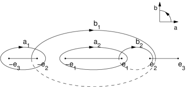
Figure 1:

We find that

$$2\Omega_{1,1}=\int_{a_{1}}\frac{dz}{w}=-\omega_{2},\qquad 2\Omega_{1,2}=\int_{a_{2}}\frac{dz}{w}=2\omega_{2},$$

$$2\Omega_{2,1}=\int_{a_{1}}\frac{zdz}{w}=\omega_{1},\qquad 2\Omega_{2,2}=\int_{a_{2}}\frac{zdz}{w}=0,$$

$$2\Omega_{1,1}^{\prime}=\int_{b_{1}}\frac{dz}{w}=0,\qquad 2\Omega_{1,2}^{\prime}=\int_{b_{2}}\frac{dz}{w}=\omega_{2}^{\prime},$$

$$2\Omega_{2,1}^{\prime}=\int_{b_{1}}\frac{zdz}{w}=2\omega_{1}^{\prime},\qquad 2\Omega_{2,2}=\int_{b_{2}}\frac{zdz}{w}=\omega_{1}^{\prime},$$

where the $\omega_{i}$ are calculated from the the homology basis shown in Figs. 2 and 3,

$$\omega_{1}=\int_{\xi_{2}^{2}}^{\xi_{3}^{2}}\frac{dx}{w_{1}},\qquad\omega_{1}^{\prime}=\int_{\xi_{1}^{2}}^{\xi_{2}^{2}}\frac{dx}{w_{1}},\qquad\omega_{2}=\int_{\xi_{2}^{2}}^{\xi_{3}^{2}}\frac{dx}{w_{2}},\qquad\omega_{2}^{\prime}=\int_{\xi_{1}^{2}}^{\xi_{2}^{2}}\frac{dx}{w_{2}}.$$

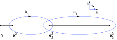
Figure 2:

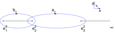
Figure 3:

Proof

Using the change of variable $z^{2}=x$, $2zdz=dx$, we have

$$2\Omega_{1,1}=\int_{a_{1}}\frac{dz}{w}=\int_{-e_{3}}^{-e_{2}}\frac{2dz}{w}=\int_{e_{3}^{2}}^{e_{2}^{2}}\frac{dx}{\sqrt{x(x-\xi_{1}^{2})(x-\xi_{2}^{2})(x-\xi_{3}^{2})}}$$

$$\phantom{2\Omega_{1,1}}{}=-\int_{e_{2}^{2}}^{e_{3}^{2}}\frac{dx}{\sqrt{x(x-\xi_{1}^{2})(x-\xi_{2}^{2})(x-\xi_{3}^{2})}}=-\omega_{2},$$

$$2\Omega_{1,2}=\int_{a_{2}}\frac{dz}{w}=\int_{-e_{1}}^{0}\frac{2dz}{w}+\int^{e_{1}}_{0}\frac{2dz}{w}=2\int_{0}^{e_{1}^{2}}\frac{dx}{\sqrt{x(x-\xi_{1}^{2})(x-\xi_{2}^{2})(x-\xi_{3}^{2})}}=$$

$$\phantom{2\Omega_{1,2}}{}=2\int_{e_{2}^{2}}^{e_{3}^{2}}\frac{dx}{\sqrt{x(x-\xi_{1}^{2})(x-\xi_{2}^{2})(x-\xi_{3}^{2})}}=2\omega_{2},$$

$$2\Omega_{2,1}=\int_{a_{1}}\frac{zdz}{w}=\int_{-e_{3}}^{-e_{2}}\frac{2zdz}{w}=\int_{e_{3}^{2}}^{e_{2}^{2}}\frac{dx}{\sqrt{(x-\xi_{1}^{2})(x-\xi_{2}^{2})(x-\xi_{3}^{2})}}$$

$$\phantom{2\Omega_{2,1}}{}=-\int_{e_{2}^{2}}^{e_{3}^{2}}\frac{dx}{\sqrt{(x-\xi_{1}^{2})(x-\xi_{2}^{2})(x-\xi_{3}^{2})}}=-\omega_{1},$$

$$2\Omega_{2,2}=\int_{a_{2}}\frac{zdz}{w}=\int_{-\xi}^{0}\frac{2zdz}{w}+\int^{\xi}_{0}\frac{2zdz}{w}=0\qquad\text{by symmetry under}\qquad z\rightarrow-z,$$

and

$$2\Omega_{1,1}^{\prime}=\int_{b_{1}}\frac{dz}{w}=0\qquad\text{(by symmetry)},$$

$$2\Omega_{1,2}^{\prime}=\int_{b_{2}}\frac{dz}{w}=\int_{e_{1}}^{e_{2}}\frac{2dz}{w}=\int_{e_{1}^{2}}^{e_{2}^{2}}\frac{dx}{\sqrt{x(x-\xi_{1}^{2})(x-\xi_{2}^{2})(x-\xi_{3}^{2})}}=\omega_{2},$$

$$2\Omega_{2,1}^{\prime}=\int_{b_{1}}\frac{zdz}{w}=2\int_{e_{1}}^{e_{2}}\frac{2zdz}{w}=2\omega_{1}\qquad\text{(as for $\Omega_{2,2}^{\prime}$)},$$

$$2\Omega_{2,2}^{\prime}=\int_{b_{2}}\frac{zdz}{w}=\int_{e_{1}}^{e_{2}}\frac{2zdz}{w}=\int_{e_{1}^{2}}^{e_{2}^{2}}\frac{dx}{\sqrt{(x-\xi_{1}^{2})(x-\xi_{2}^{2})(x-\xi_{3}^{2})}}=\omega_{1}.$$

The $\omega$ can be calculated by standard integrals

$$\omega_{1}=\int_{e_{2}^{2}}^{e_{3}^{2}}\frac{dx}{\sqrt{(x-\xi_{1}^{2})(x-\xi_{2}^{2})(x-\xi_{3}^{2})}}=\frac{2i}{\sqrt{\xi_{3}^{2}-\xi_{1}^{2}}}\,K\left(\sqrt{\frac{\xi_{3}^{2}-\xi_{2}^{2}}{\xi_{3}^{2}-\xi_{1}^{2}}}\right),$$

$$\omega_{1}^{\prime}=\int_{e_{1}^{2}}^{e_{2}^{2}}\frac{dx}{\sqrt{(x-\xi_{1}^{2})(x-\xi_{2}^{2})(x-\xi_{3}^{2})}}=\frac{2}{\sqrt{\xi_{3}^{2}-\xi_{1}^{2}}}\,K\left(\sqrt{\frac{\xi_{2}^{2}-\xi_{1}^{2}}{\xi_{3}^{2}-\xi_{1}^{2}}}\right),$$

$$\omega_{2}=\int_{e_{2}^{2}}^{e_{3}^{2}}\frac{dx}{\sqrt{x(x-\xi_{1}^{2})(x-\xi_{2}^{2})(x-\xi_{3}^{2})}}=\frac{2i}{\sqrt{(\xi_{3}^{2}-\xi_{1}^{2})\xi_{2}^{2}}}\,K\left(\sqrt{\frac{(\xi_{3}^{2}-\xi_{2}^{2})\xi_{1}^{2}}{(\xi_{3}^{2}-\xi_{1}^{2})\xi_{2}^{2}}}\right),$$

$$\omega_{2}^{\prime}=\int_{e_{1}^{2}}^{e_{2}^{2}}\frac{dx}{\sqrt{x(x-\xi_{1}^{2})(x-\xi_{2}^{2})(x-\xi_{3}^{2})}}=\frac{2}{\sqrt{(\xi_{3}^{2}-\xi_{1}^{2})\xi_{2}^{2}}}\,K\left(\sqrt{\frac{(\xi_{2}^{2}-\xi_{1}^{2})\xi_{3}^{2}}{(\xi_{3}^{2}-\xi_{1}^{2})\xi_{2}^{2}}}\right)$$

so the period matrices we obtain can be written in the form

$$\Omega=\left[\begin{matrix}-\dfrac{1}{2}\omega_{2}&\omega_{2}\\ \omega_{1}&0\end{matrix}\right],\qquad\Omega^{\prime}=\left[\begin{matrix}0&\dfrac{1}{2}\omega_{2}^{\prime}\\[8.61108pt] \omega_{1}^{\prime}&\dfrac{1}{2}\omega_{1}^{\prime}\end{matrix}\right],$$

so

$$\tau=\left[\begin{matrix}2\dfrac{\omega_{1}}{\omega_{1}^{\prime}}&\dfrac{\omega_{1}}{\omega_{1}^{\prime}}\\[8.61108pt] \dfrac{\omega_{1}}{\omega^{\prime}}&\dfrac{1}{2}\dfrac{\omega_{2}}{\omega_{2}^{\prime}}+\dfrac{1}{2}\dfrac{\omega_{1}}{\omega_{1}^{\prime}}\end{matrix}\right]=\left[\begin{matrix}2\tau_{1}&\tau_{1}\\[8.61108pt] \tau_{1}&\dfrac{1}{2}\tau_{2}+\dfrac{1}{2}\tau_{1}\end{matrix}\right].$$

Following Martens, if we define

$$m=\left[\begin{matrix}0&0&2&1\\ 1&0&0&0\end{matrix}\right]$$

then

$$\left[\begin{matrix}\omega_{1}&\omega_{1}^{\prime}\end{matrix}\right]\cdot m=2\left[\begin{matrix}0&1\end{matrix}\right]\cdot\left[\begin{matrix}\Omega&\Omega^{\prime}\end{matrix}\right].$$

Now define

$$J=\left[\begin{matrix}0_{2}&I_{2}\\ -I_{2}&0_{2}\end{matrix}\right],\qquad T=\left[\begin{matrix}0&0&2&1\\ 1&-2&0&2\\ 0&-1&0&1\\ 0&0&1&0\end{matrix}\right],$$

where $T$ is symplectic, $T\cdot J\cdot T^{t}=J$, and

$$m\cdot T^{-1}=\left[\begin{matrix}1&0&0&0\\ 0&1&-2&0\end{matrix}\right]$$

is in (Martens) standard form, and

$$m\cdot J\cdot m^{t}=\left[\begin{matrix}0&-2\\ 2&0\end{matrix}\right]$$

shows that the Hopf number is 2.

The transformed matrix $\tilde{\tau}$ is calculated by first calculating the $2\times 4$ matrix

$$\left[\begin{matrix}A&B\end{matrix}\right]=\left[\begin{matrix}I_{2}&\tau\end{matrix}\right]\cdot(J\cdot T)^{-1}$$

then

$$\tilde{\tau}=A^{-1}B=\left[\begin{matrix}\dfrac{1}{2}\tau_{1}&\dfrac{1}{2}\\[8.61108pt] \dfrac{1}{2}&-\dfrac{1}{2(2+\tau_{2})}\end{matrix}\right],$$

where $\tau_{i}=\omega_{i}^{\prime}/\omega_{i}$.

For this matrix, we use Martens’ transformation formula, generalized to non-zero characteristics:

$$\Theta\left[\begin{matrix}0&0\\[4.30554pt] {\dfrac{1}{2}}&0\end{matrix}\right]\left(\left[\begin{matrix}-\dfrac{1}{2}v_{1}\\[4.30554pt] -\dfrac{v_{1}-2v_{2}}{2(2+\tau_{2})}\end{matrix}\right],\tilde{\tau}\right)=\Theta\left[\begin{matrix}0\\[4.30554pt] {\dfrac{1}{2}}\end{matrix}\right]\biggl{(}-\frac{v_{1}}{2},\frac{\tau_{1}}{2}\biggr{)}\Theta\left[\begin{matrix}0\\[4.30554pt] 0\end{matrix}\right]\biggl{(}\frac{v_{1}-2v_{2}}{2+\tau 2},-\frac{2}{2+\tau_{2}}\biggr{)}$$

$$\qquad{}+\Theta\left[\begin{matrix}0\\[4.30554pt] 0\end{matrix}\right]\biggl{(}-\frac{v_{1}}{2},\frac{\tau_{1}}{2}\biggr{)}\Theta\left[\begin{matrix}\dfrac{1}{2}\\[4.30554pt] 0\end{matrix}\right]\biggl{(}\frac{v_{1}-2v_{2}}{2+\tau_{2}},-\frac{2}{2+\tau_{2}}\biggr{)}$$

$$\qquad{}=\dfrac{1}{2}\theta_{3}\biggl{(}\dfrac{1}{2}v_{1},\dfrac{1}{2}\tau_{1}\biggr{)}\theta_{3}\biggl{(}\dfrac{1}{2}v_{1}-v_{2},\dfrac{1}{2}\tau_{2}\biggr{)}+\dfrac{1}{2}\theta_{4}\biggl{(}\dfrac{1}{2}v_{1},\dfrac{1}{2}\tau_{1}\biggr{)}\theta_{4}\biggl{(}\dfrac{1}{2}v_{1}-v_{2},\dfrac{1}{2}\tau_{2}\biggr{)},$$

in Jacobi notation, concluding the proof.

4 Genus three

In [10], we calculated, using Halphen’s ansatz as described in Section 1 (cf. [36] as well), the Halphen spectral curve, trigonal of genus 3, for the operator: $L=\partial^{3}-15\wp\partial-({15}/{2})\wp^{\prime}=0$:

$$w^{3}=\biggl{(}z^{2}+\dfrac{25}{4}g_{3}\biggr{)}\biggl{(}z^{2}-\dfrac{135}{4}g_{3}\biggr{)}.$$

We showed that this curve not only admits reduction, but also has Jacobian isogenous to the product of three (isomorphic) elliptic curves. Here we consider the covers in the slightly more general genus 3 curve $w^{3}=(z^{2}-\lambda_{1}^{2})(z^{2}+\lambda_{2}^{2})$, $\lambda_{1},\lambda_{2}\in{\mathbb{R}}$, to curves of genus 1 and 2 and derive the corresponding $\tau$ matrices and reduction theory. On occasion we indicate results for the special case $\lambda_{1}^{2}=(135/3)g_{3}$, $\lambda_{2}^{2}=(25/4)g_{3}$:

$$\tilde{\cal{C}}_{3}:\ w^{3}=\biggl{(}z^{2}+\dfrac{25}{4}g_{3}\biggr{)}\biggl{(}z^{2}-\dfrac{135}{4}g_{3}\biggr{)}.$$

This genus 3 curve covers the equianharmonic elliptic curve $(\wp^{\prime})^{2}=4\wp^{3}-g_{3}$ in three different ways and all entries to the period matrices are expressible in terms of the modulus of this curve. For the specific curve $\tilde{\cal{C}}_{3}$, we have three covers, all covering $(\wp^{\prime})^{2}=4\wp^{3}-g_{3}$, as follows.

The cover $\pi_{1}$ is given by

$$\wp=\frac{w^{2}}{25}\frac{(16z^{2}+8100g_{3})}{(4z^{2}-135g_{3})^{2}},\qquad\wp^{\prime}=\frac{2}{125}\frac{z(16z^{4}-19000z^{2}g_{3}-759375g_{3}^{2})}{(4z^{2}-135g_{3})^{2}}$$

with holomorphic differentials given by

$$\frac{dz}{w}=\frac{3}{5}\frac{d\wp}{\wp^{\prime}}.$$

The cover $\pi_{2}$ is given by

$$\wp=\frac{\sqrt[3]{5}w}{20\sqrt[3]{-g_{3}}},\qquad\wp^{\prime}=\frac{4z^{2}-55g_{3}}{80\sqrt[3]{-g_{3}}}$$

with holomorphic differentials given by

$$\dfrac{zdz}{w^{2}}=\dfrac{3d\wp}{4\root 3 \of{5}\root 6 \of{-g_{3}}\wp^{\prime}}.$$

The cover $\pi_{3}$ is given by

$$\wp=-\frac{1}{4800}\frac{w\sqrt[3]{5}(64{z}^{6}-80\,g_{3}{z}^{4}-5300g_{3}^{2}{z}^{2}-30375g_{3}^{3})}{(-g_{3})^{4/3}{z}^{2}(4\,{z}^{2}+25\,g_{3})},$$

$$\wp^{\prime}=\frac{-ip_{10}}{1152000(4{z}^{2}+25g_{3}){z}^{3}{g_{3}}^{2}},$$

where

$$p_{10}=\big{(}-61509375\,{g_{3}}^{5}-15187500{z}^{2}{g_{3}}^{4}-700000{z}^{4}{g_{3}}^{3}-240000{z}^{6}{g_{3}}^{2}$$

$$\phantom{p_{10}=}{}-19200{z}^{8}g_{3}+1024{z}^{10}\big{)}\sqrt{15}$$

with holomorphic differentials given by

$$\frac{dz}{w^{2}}=\frac{i{d\wp}\sqrt{15}\,{5}^{2/3}}{250\wp(-g_{3})^{2/3}}.$$

The general curve ${\cal C}_{3}$ is a covering of the equianharmonic elliptic curve $\cal{C}_{1}$ given by the equation

$$\nu^{2}=4\mu^{3}+(\lambda_{1}^{2}+\lambda_{2}^{2})^{2}.$$

The cover $\pi$ is given by

$$\mu=w,\qquad\nu=2z^{2}+\lambda_{2}^{2}-\lambda_{1}^{2},$$

with holomorphic differentials given by

$$\dfrac{2zdz}{3w^{2}}=\dfrac{d\mu}{\nu}.$$

4.1 Reduction

In this section we follow a similar approach to that of Matsumoto [21] in a genus 4 problem, who developed earlier results of Shiga [28] and Picard [23]. Write the equation of ${\cal C}$ in the form

$$w^{3}=\prod_{k=1}^{4}(z-\lambda_{k})=(z-\lambda_{1})(z+\lambda_{1})(z-i\lambda_{2})(z+i\lambda_{2}).$$

We fix the following lexicographical ordering of independent canonical holomorphic differentials of ${\cal C}_{3}$, ${d}u_{1}={{d}z/w}$, ${d}u_{2}={{d}z/w^{2}}$, ${d}u_{3}={z{d}z/w^{2}},$ and will define the period matrix based on the branch cuts given in Figs. 4 and 5.

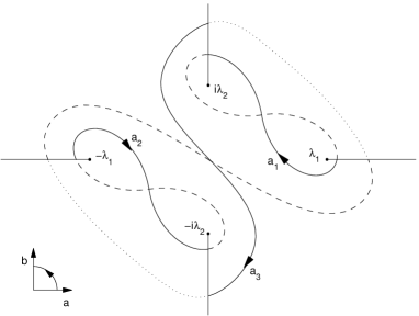
Figure 4:

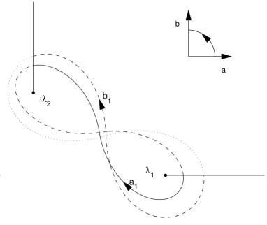
Figure 5:

4.2 Riemann period matrix

We introduce the following vector notation:

$${\bf x}=(x_{1},x_{2},x_{3})^{T}=\left(\oint_{{a}_{1}}{d}u_{1},\ldots,\oint_{{a}_{3}}{d}u_{1}\right)^{T},$$

$${\bf b}=(b_{1},b_{2},b_{3})^{T}=\left(\oint_{{a}_{1}}{d}u_{2},\ldots,\oint_{{a}_{3}}{d}u_{2}\right)^{T},$$

$${\bf c}=(c_{1},c_{2},c_{3})^{T}=\left(\oint_{{a}_{1}}{d}u_{3},\ldots,\oint_{{a}_{3}}{d}u_{3}\right)^{T}.$$

Then the matrices of ${a}$ and ${b}$-periods read

$$\mathcal{A}=\Biggl{(}\oint_{\mathfrak{a}_{k}}\mathrm{d}u_{i}\Biggr{)}_{i,k=1,\ldots,3}=(\boldsymbol{x},\boldsymbol{b},\boldsymbol{c}),$$ (2)

$$\mathcal{B}=\Biggl{(}\oint_{\mathfrak{b}_{k}}\mathrm{d}u_{i}\Biggr{)}_{i,k=1,\ldots,3}=(\rho H\boldsymbol{x},\rho^{2}H\boldsymbol{b},\rho^{2}H\boldsymbol{c}),$$ (3)

where $H={\rm diag}(1,1,-1)$. The Riemann bilinear relation says

$${\bf x}^{T}H{\bf b}={\bf x}^{T}H{\bf c}=0.$$

The Riemann period matrix $\tau={\cal{A}}{\cal{B}}^{-1}$ belongs to the Siegel upper half-space ${\mathbb{H}}^{3}$.

By using the symmetries of the problem we can express all the ${\bf x}$ period integrals in terms of the two integrals (see Fig. 6)

$$I=\int_{0}^{\lambda_{1}}\dfrac{dz}{w},\qquad J=\int_{0}^{i\lambda_{2}}\dfrac{dz}{w}.$$

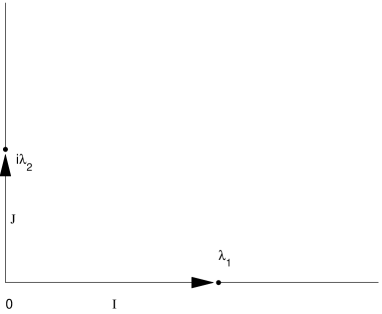
Figure 6: Paths of $I$ and $J$ integrals on sheet 1. To get the corresponding integrals on the other sheets we multiply by $\rho$ and $\rho^{2}$ respectively. The $a$ and $b$ contours can be constructed by pasting together various combinations of these integrals and their reflections in the real and imaginary axes.

We have

$$x_{1}=(\rho^{2}-1)(I-J),\qquad x_{2}=-x_{1},\qquad x_{3}=-2J+\rho(J-I)+2\rho^{2}I+\rho(J-I),$$

where $\rho=\exp\{2i\pi/3\}$. In the case when $\lambda_{2}^{2}/\lambda_{1}^{2}=5/27$, the integrals simplify further, since $I=-J(1+2\rho)/3$. In this case (which we assume in all that follows) we have

$$x_{1}=2J(\rho+1),\qquad x_{2}=-x_{1},\qquad x_{3}=2J(\rho-2).$$

So we have

$$\left[(\Omega^{\prime})^{T}\Omega^{T}\right]=\left[\begin{matrix}-2\,J&2J&2J(3\rho+1)&2J\rho_{1}&-2J\rho_{1}&2J(\rho-2)\\[2.15277pt] -\rho_{1}b_{{1}}&-\rho_{1}b_{2}&\rho_{1}b_{3}&b_{1}&b_{2}&b_{3}\\[2.15277pt] -(\rho+1)c_{1}&-(\rho+1)c_{2}&\rho_{1}c_{3}&c_{1}&c_{2}&c_{3}\end{matrix}\right],$$

where $\rho_{1}=\rho+1$. We define

$$\tau=((\Omega^{\prime})^{T})^{-1}\Omega^{T}.$$

We find after much simplification, using the properties of $\rho$ and the Riemann relations, that

$$\tau=\frac{1}{79}\left[\begin{matrix}62\rho-13&17\rho+13&-5\rho+38\\[2.15277pt] 17\rho+13&62\rho-13&5\rho-38\\[2.15277pt] -5\rho+38&5\rho-38&45\rho+53\end{matrix}\right].$$

This matrix $[(\Omega^{\prime})^{T}\,\Omega^{T}]$ satisfies the reduction criteria as defined by Martens [20], since if we define

$$\Pi=\left[\begin{matrix}2J&2J\rho\end{matrix}\right],\qquad H=\left[\begin{matrix}1&0&0\end{matrix}\right],$$

then

$$H\cdot\left[(\Omega^{\prime})^{T}\ \Omega^{T}\right]=\Pi\cdot M,$$

where

$$M=\left[\begin{matrix}-1&1&1&1&-1&-2\\[2.15277pt] 0&0&3&1&-1&1\end{matrix}\right].$$

We can transform $M$ to standard form using the symplectic matrix

$$S=\left[\begin{matrix}1&3&-1&0&-6&2\\[2.15277pt] 0&-1&-1&0&1&-1\\[2.15277pt] 0&1&0&-3&-1&0\\[2.15277pt] 0&0&0&1&0&0\\[2.15277pt] 0&0&0&-1&0&-1\\[2.15277pt] 0&-2&0&2&3&-1\end{matrix}\right],$$

since

$$M.S=\left[\begin{array}[]{cccccc}-1&0&0&0&0&0\\ \vskip 6.0pt plus 2.0pt minus 2.0pt\cr 0&1&0&-5&0&0\end{array}\right].$$

Following Martens, the corresponding transformed $\tau$ is

$$\tilde{\tau}=\tau\cdot S\cdot J^{T}=\left[\begin{matrix}\dfrac{1}{5}+\dfrac{1}{5}\,\rho&\dfrac{1}{5}&0\\[8.61108pt] \dfrac{1}{5}&\dfrac{1}{2}+\dfrac{1}{5}\,\rho&\dfrac{1}{2}\,\rho\\[8.61108pt] 0&\dfrac{1}{2}\,\rho&\dfrac{3}{2}\,\rho+\dfrac{1}{2}\end{matrix}\right].$$

Expanding a theta function defined with this $\tilde{\tau}$, again following Martens, we will get a sum of 5 products of $g=1$ theta functions with $g=2$ theta functions. The $g=1$ theta functions will have tau value $\tau=(1/5)(1+\rho)$ and the $g=2$ theta functions will have a tau of

$$\tau=\left[\begin{matrix}5&0\\[8.61108pt] 0&1\end{matrix}\right]\left[\begin{matrix}\dfrac{1}{2}+\dfrac{1}{5}\,\rho&\dfrac{1}{2}\,\rho\\[8.61108pt] \dfrac{1}{2}\,\rho&\dfrac{3}{2}\,\rho+\dfrac{1}{2}\end{matrix}\right]\left[\begin{matrix}5&0\\[8.61108pt] 0&1\end{matrix}\right]=\left[\begin{matrix}5\,\rho+{\dfrac{25}{2}}&\dfrac{5}{2}\,\rho\\[8.61108pt] \dfrac{5}{2}\,\rho&\dfrac{3}{2}\,\rho+\dfrac{1}{2}\end{matrix}\right].$$

Again following Martens, we can reduce this $2\times 2$ matrix to standard form to get eventually

$$\tilde{\tilde{\tau}}=\left[\begin{array}[]{cc}\dfrac{11}{20}+\dfrac{1}{20}\,\rho&-\dfrac{1}{4}\\ \vskip 6.0pt plus 2.0pt minus 2.0pt\cr-\dfrac{1}{4}&\dfrac{3}{2}+\dfrac{1}{4}\,\rho\end{array}\right].$$

Expanding each of the transformed genus 2 theta functions with this theta will give a product of genus 1 theta functions with $\tau=(1/20)(11+\rho)$ and genus 1 theta functions with $\tau=16({3/2}+(1/4)\,\rho)$. So finally we have $5\cdot 4=20$ terms, each containing a product of three genus 1 theta functions (with fractional characteristics).

5 Conclusions

We contributed to the theory of spectral curves of ODOs with elliptic coefficients routine algorithms to calculate:

• The algebraic equation of the curve (always, in principle);

• The period matrix (only if the periods can be chosen suitably and there is an explicit solution to the action equations);

• A reduction method for the theta function.

What remains to be calculated (Challenge IV) is the dependence of the coefficients on the time parameters. This is more difficult because it involves expanding an entire basis of differentials of the first kind. In [10], we were able to find the time dependence by implementing Jacobi inversion, thanks to the Hamiltonian-system theory which describes the evolution of the poles of the KP solution [18].

References

- [1]
- [2] Arscott F.M., Periodic differential equations. An introduction to Mathieu, Lamé, and Allied functions, International Series of Monographs in Pure and Applied Mathematics, Vol. 66, A Pergamon Press Book, The Macmillan Co., New York, 1964.
- [3] Baker H.F., An introduction to the theory of multiply-periodic functions, University Press XVI, Cambridge, 1907.
- [4] Belokolos E.D., Enolskii V.Z., Reduction of Abelian functions and algebraically integrable systems. I, in Complex Analysis and Representation Theory, 2, J. Math. Sci. 106 (2001), 3395–3486.
- [5] Belokolos E.D., Enolskii V.Z., Reduction of Abelian functions and algebraically integrable systems. II, in Complex Analysis and Representation Theory, 3, J. Math. Sci. 108 (2002), 295–374.
- [6] Buchstaber V.M., Enol’skiĭ V.Z., Leĭkin D.V., Hyperelliptic Kleinian functions and applications, in Solitons, geometry, and topology: on the crossroad, Amer. Math. Soc. Transl. Ser. 2, Vol. 179, Amer. Math. Soc., Providence, RI, 1997, 1–33, solv-int/9603005.
- [7] Earle C.J., The genus two Jacobians that are isomorphic to a product of elliptic curves, in The Geometry of Riemann Surfaces and Abelian Varieties, Contemp. Math. 397 (2006), 27–36.
- [8] Eilbeck J.C., Ènol’skiĭ V.Z., Elliptic Baker–Akhiezer functions and an application to an integrable dynamical system, J. Math. Phys. 35 (1994), 1192–1201.
- [9] Eilbeck J.C., Enol’skii V.Z., Some applications of computer algebra to problems in theoretical physics, Math. Comput. Simulation 40 (1996), 443–452.
- [10] Eilbeck J.C., Enolskii V.Z., Previato E., Varieties of elliptic solitons, J. Phys. A: Math. Gen. 34 (2001), 2215–2227.
- [11] Flédrich P., Treibich A., Hyperelliptic osculating covers and KdV solutions periodic in , Int. Math. Res. Not. 2006 (2006), Art. ID 73476, 17 pages.
- [12] Gesztesy F., Weikard R., Elliptic algebro-geometric solutions of the KdV and AKNS hierarchies – an analytic approach, Bull. Amer. Math. Soc. (N.S.) 35 (1998), 271–317, solv-int/9809005.
- [13] Gesztesy F., Weikard R., A characterization of all elliptic algebro-geometric solutions of the AKNS hierarchy, Acta Math. 181 (1998), 63–108, solv-int/9705018.
- [14] Grosset M.-P., Veselov A.P., Elliptic Faulhaber polynomials and Lamé densities of states, Int. Math. Res. Not. 2006 (2006), Art. ID 62120, 31 pages, math-ph/0508066.
- [15] Halphen M., Traité des fonctions elliptiques et des leurs applications, Gauthier-Villars Paris, 1888.
- [16] Kani E., Elliptic curves on abelian surfaces, Manuscripta Math. 84 (1994), 199–223.
- [17] Kennedy D.H., Little sparrow: a portrait of Sophia Kovalevsky, Ohio University Press, Athens, OH, 1983.
- [18] Krichever I.M., Elliptic solutions of the Kadomcev–Petviašvili equations, and integrable systems of particles, Funktsional. Anal. i Prilozhen 14 (1980), 45–54 (English transl.: Funct. Anal. Appl. 14 (1980), 282–290).
- [19] Maier R.S., Lamé polynomials, hyperelliptic reductions and Lamé band structure, Philos. Trans. R. Soc. Lond. Ser. A Math. Phys. Eng. Sci., to appear, math-ph/0309005.
- [20] Martens H.H., A footnote to the Poincaré complete reducibility theorem, Publ. Mat. 36 (1992), 111–129.
- [21] Matsumoto K., Theta constants associated with the cyclic triple coverings of the complex projective line branching at six points, Publ. Res. Inst. Math. Sci. 37 (2001), 419–440, math.AG/0008025.
- [22] Matveev V.B., Smirnov A.O., On the link between the Sparre equation and Darboux–Treibich–Verdier equation, Lett. Math. Phys. 76 (2006), 283–295.
- [23] Picard E., Sur les fonctions de deux variables indépendentes analogues aux fonctions modulaires, Acta Math. 2 (1883), 114–135.
- [24] Prapavessi D.T., On the Jacobian of the Klein curve, Proc. Amer. Math. Soc. 122 (1994), 971–978.
- [25] Previato E., Another algebraic proof of Weil’s reciprocity, Atti Accad. Naz. Lincei Cl. Sci. Fis. Mat. Natur. Rend. (9) Mat. Appl. 2 (1991), 167–171.
- [26] Rauch H.E., Lewittes J., The Riemann surface of Klein with 168 automorphisms, in Problems in Analysis (papers dedicated to Salomon Bochner, 1969), Princeton Univ. Press, Princeton, NJ, 1970, 297–308.
- [27] Quine J.R., Jacobian of the Picard curve, in Extremal Riemann Surfaces (1995, San Francisco, CA), Contemp. Math. 201 (1997), 33–41.
- [28] Shiga H., On the representation of the Picard modular function by constants I–II, Publ. Res. Inst. Math. Sci. 24 (1988), 311–360.
- [29] Segal G., Wilson G., Loop groups and equations of KdV type, Inst. Hautes Études Sci. Publ. Math. 61 (1985), 5–65.
- [30] Shaska T., Völklein H., Elliptic subfields and automorphisms of genus 2 function fields, in Algebra, Arithmetic and Geometry with Applications (West Lafayette, IN, 2000), Springer, Berlin, 2004, 703–723, math.AG/0107142.
- [31] Smirnov A.O., Solutions of the KdV equation that are elliptic in , Teoret. Mat. Fiz. 100 (1994), no. 2, 183–198 (English transl.: Theoret. and Math. Phys. 100 (1994), no. 2, 937–947).
- [32] Takemura K., The Heun equation and the Calogero–Moser–Sutherland system. I. The Bethe Ansatz method, Comm. Math. Phys. 235 (2003), 467–494, math.CA/0103077.
- [33] Takemura K., The Heun equation and the Calogero–Moser–Sutherland system. II. Perturbation and algebraic solution, Electron. J. Differential Equations (2004), No. 15, 30 pages, math.CA/0112179.
- [34] Takemura K., The Heun equation and the Calogero–Moser–Sutherland system. III. The finite-gap property and the monodromy, J. Nonlinear Math. Phys. 11 (2004), 21–46, math.CA/0201208.
- [35] Takemura K., The Heun equation and the Calogero–Moser–Sutherland system. IV. The Hermite–Krichever ansatz, Comm. Math. Phys. 258 (2005), 367–403, math.CA/0406141.
- [36] Unterkofler K., On the solutions of Halphen’s equation, Differential Integral Equations 14 (2001), 1025–1050.
- [37] Whittaker E.T., Watson G.N., A course of modern analysis. An introduction to the general theory of infinite processes and of analytic functions; with an account of the principal transcendental functions, Reprint of the fourth (1927) edition, Cambridge University Press, Cambridge, 1996.
- [38] Yuzbashyan E.A., Altshuler B.L., Kuznetsov V.B., Enolskii V.Z., Solution for the dynamics of the BCS and central spin problems, J. Phys. A: Math. Gen. 38 (2005), 7831–7849, cond-mat/0407501.