Complex zeros of eigenfunctions of 1D Schrödinger operators

Abstract.

In this article we study the semi-classical distribution of the complex zeros of the eigenfunctions of the 1D Schrödinger operators for the class of real polynomial potentials of even degree, with fixed energy level, $E$. We show that as $h_{n}\to 0$ the zeros tend to concentrate on the union of some level curves $\Re(S(z_{m},z))=c_{m}$ where $S(z_{m},z)=\int_{z_{m}}^{z}\sqrt{V(t)-E}\,dt$ is the complex action, and $z_{m}$ is a turning point. We also calculate these curves for some symmetric and non-symmetric one-well and double-well potentials. The example of the non-symmetric double-well potential shows that we can obtain different pictures of complex zeros for different subsequences of $h_{n}$.

Keywords: Schrodinger operator, Complex WKB method, Stokes lines.

1. Introduction

This article is concerned with the eigenvalue problem for a one-dimensional semi-classical Schrödinger operator

(1) $$(-h^{2}\frac{d^{2}}{dx^{2}}+V(x))\psi(x,h)=E(h)\psi(x,h),\qquad\psi(x,h)\in L^{2}({\mathbb{R}})\quad h\to 0^{+}$$

Using the spectral theory of the Shrödinger operators [BS], we know that if $\lim_{x\to\underline{+}\infty}V(x)=+\infty$ then the spectrum is discrete and can be arranged in an increasing sequence $E_{0}(h)<E_{1}(h)<E_{2}(h)<\cdots\uparrow\infty$. Notice that each eigenvalue has multiplicity one. We let $\{\psi_{n}(x,h)\}$ be a sequence of eigenfunctions associated to $E_{n}(h)$. If we assume the potential $V(x)$ is a real polynomial of even degree with positive leading coefficient, then we can arrange the eigenvalues as above and the eigenfunctions $\psi_{n}(x,h)$ possess analytic continuations $\psi_{n}(z,h)$ to ${\mathbb{C}}$. Our interest is in the distribution of complex zeros of $\psi_{n}(z,h)$ as $h\to 0^{+}$ when an energy level $E$ is fixed. The substitutions $\lambda=\frac{1}{h}$, and $q(x)=V(x)-E$ changes the eigenvalue problem (1) to the problem:

(2) $$y^{\prime\prime}(x,\lambda)=\lambda^{2}q(x)y(x,\lambda),\qquad y(x,\lambda)\in L^{2}({\mathbb{R}}),\qquad\lambda\to\infty.$$

Since $\lim_{x\to\underline{+}\infty}q(x)=+\infty$, again the spectrum is discrete and can be arranged as

(3) $$\lambda_{0}<\lambda_{1}<\lambda_{2}<\cdots<\lambda_{n}\cdots\uparrow\infty.$$

We define the discrete measure $Z_{\lambda_{n}}$ by

(4) $$Z_{\lambda_{n}}=\frac{1}{\lambda_{n}}\sum_{\{z|\;y(z,\lambda_{n})=0\}}\delta_{z}.$$

In this paper we study the limits of weak^∗ convergent subsequences of the sequence $\{Z_{\lambda_{n}}\}$ as $n\to\infty$. We say

$$Z_{\lambda_{n_{k}}}\longrightarrow Z,\quad(\text{in weak}^{*}\;\text{sense})$$

if for every test function $\varphi\in C_{c}^{\infty}(\mathbb{R}^{2})$ we have

$$Z_{\lambda_{n_{k}}}(\varphi)\longrightarrow Z(\varphi).$$

We will call these weak limits, the zero limit measures.

Throughout this article we assume that $q(z)$ has simple zeros. We may be able to extend the results in the case of multiple turning points using the methods in [F1, O2] on the asymptotic expansions around multiple turning points. Notice that $q(x)$ has to change its sign on the real axis, because if it is positive everywhere then (2) does not have any solution in $L^{2}({\mathbb{R}})$. Hence $q(z)$ has at least two simple real zeros. We say $q(x)$ is a one-well potential if it has exactly two (simple) real zeros and a double-well potential if it has exactly four (simple) real zeros. One of our results is

Theorem 1.1.

Let $q(z)$ be a real polynomial of even degree with positive leading coefficient. Then every weak limit $Z$ (zero limit measure) of the sequence $\{Z_{\lambda_{n}}\}$ is of the form

(5) $$Z=\frac{1}{\pi}|\sqrt{q(z)}|\,|d\gamma|,$$

$$|d\gamma|=|\gamma^{\prime}(t)|\,dt,$$

where $\gamma$ is a union of finitely many smooth connected curves $\gamma_{m}$ in the plane. For each $\gamma_{m}$ there exists a constant $c_{m}$, a canonical domain $D_{m}$ and a turning point $z_{m}$ on the boundary of $D_{m}$ such that $\gamma_{m}$ is given by

(6) $$\Re(S(z_{m},z))=c_{m},\qquad z\in D_{m},$$

where $S(z_{m},z)=\int_{z_{m}}^{z}\sqrt{q(t)}\,dt$ and the integral is taken along any path in $D_{m}$ joining $z_{m}$ to $z$.(See section 2, for the definitions)

This theorem shows that if $Z$ in (5) is the limit of a subsequence $\{Z_{\lambda_{n_{k}}}\}$, then the complex zeros of $\{y(z,\lambda_{n_{k}})\}$ tend to concentrate on $\gamma$ as $k\to\infty$ and in the limit they cover $\gamma$. The factor $|\sqrt{q(z)}|=|\sqrt{V(z)-E}|$ indicates that the limit distribution of the zeros on $\gamma$ is measured by the Agmon metric. We call the curves $\gamma_{m}$ the zeros lines of the limit $Z$. The next question after seeing Theorem 1.1 is ”what are all the possible zero limit measures and corresponding zero lines for a given polynomial $q(z)$?” We answer this question for some one-well and double-well potentials. But before stating these results let us mention some background and motivation for the problem.

Form the classical Sturm-Liouville theory we know everything about the real zeros of solutions of (2). We know that on a classical interval (i.e. an interval where $q(x)<0$), every real-valued solution $y(x,\lambda)$ of (2) (not necessarily $L^{2}$-solution) is oscillatory and becomes highly oscillatory as $\lambda\to\infty$. In fact the spacing between the real zeros on a classical interval is $\frac{\pi}{\lambda}$. On the other hand there is at most one real zero on each connected forbidden interval where $q(x)>0$. This shows that every limit $Z$ in (5) has the union of classical intervals in its support.

It turns out that other than the harmonic oscillator $q(z)=z^{2}-a^{2}$ where the eigenfunctions do not have any non-real zeros, the complex zeros are more complicated. It is easy to see that when $q(z)=z^{4}+az^{2}+b$, the eigenfunctions have infinitely many zeros on the imaginary axis. For $q(z)=z^{4}\underline{+}a^{4}$, Titchmarsh in [T] made a conjecture that all the non-real zeros are on the imaginary axis. This conjecture was proved by Hille in [H1]. In general one can only hope to study the asymptotics of large zeros of $y(z,\lambda)$ rather than finding the exact locations of zeros. The asymptotics of zeros of solutions to (2) for a fixed $\lambda$ and large $z$, have been extensively studied mainly by E. Hille, R. Nevanlinna, H. Wittich and S. Bank (see [N], [W], [B]). But it seems the semi-classical limit of complex zeros has not been studied in the literature, at least not from the perspective that was mentioned in Theorem 1.1, which is closely related to the quantum limits of eigenfunctions. This problem was raised around fifteen years ago when physicists were trying to find a connection between eigenfunctions of quantum systems and the dynamics of the classical system. It was noticed that for the ergodic case the complex zeros tend to distribute uniformly in the phase space but for the integrable systems the zeros tend to concentrate on one-dimensional lines. An article which made this point and contains very interesting graphics is [LV]. The problem of complex zeros of complexified eigenfunctions and relations to quantum limits is suggested by S. Zelditch mainly in [Z]. There, the author proves that if a sequence $\{\varphi_{\lambda_{n}}\}$ of eigenfunctions of the Laplace-Beltrami operator on a real analytic manifold $M$ is quantum ergodic then the sequence $\{Z_{\lambda_{n}}\}$ of zero distributions associated to the complexified eigenfunctions $\{\varphi_{\lambda_{n}}^{\mathbb{C}}\}$ on $M^{\mathbb{C}}$, the complexification of $M$, is weakly convergent to an explicitly calculable measure. A natural problem is to generalize the results in [Z] for Schrödinger eigenfunctions on real analytic manifolds. This is indeed a difficult problem. Perhaps the first step to study such a problem is to consider the one dimensional case which we do in this paper. The main reason to study the complex zeros rather than the real zeros is that the problem is much easier in this case (in higher dimensions). For example in studying the zeros of polynomials as a model for eigenfunctions, the Fundamental Theorem of Algebra and Hilbert’s Nullstellensatz are two good examples of how the complex zeros are easier and somehow richer. See [Z1] for some background of the problem and some motivation in higher dimensions.

One of our results is that for a symmetric quartic oscillator the full sequence $\{Z_{\lambda_{n}}\}$ is convergent, i.e. there is a unique zero limit measure. Here, by $q(z)$ being symmetric we mean that after a translation on the real axis, q(z) is an even function. But for a non-symmetric quartic oscillator there are at least two zero limit measures. The Stokes lines play an important role in the description of the zero lines. In fact the infinite zero lines are asymptotic to Stokes lines. This fact was observed in [B].

Our proofs are elementary. We use the complex WKB method, connection formulas and asymptotics of the eigenvalues by Fedöryuk in [F1].

At the end of the paper (3.2) we will briefly mention some interesting examples of one-well and double-well potentials where deg$(q(z))=4,6$.

Theorem 1.2.

Let $q(z)=(z^{2}-a^{2})(z^{2}-b^{2})$, where $0<a<b$. Then as $n\to\infty$

$$Z_{\lambda_{n}}\longrightarrow\frac{1}{\pi}|\sqrt{q(z)}|\,|d\gamma|,\qquad\gamma=(a,b)\cup(-b,-a)\cup(-\infty i,+\infty i).$$

Notice in Theorem 1.2 we can express $\gamma$ by three equations

$$\gamma=\{\Re S(a,z)=0\}\cup\{\Re S(-a,z)=0\}\cup\{\Re S(a,z)=-{\frac{1}{2}}\xi\},$$

where $\xi=\int_{-a}^{a}\sqrt{q(t)}\,dt$, and each equation is written in some canonical domain.

Theorem 1.3.

Let $q(z)=(z^{2}-a^{2})(z^{2}+b^{2})$, where $a,b>0$. Then as $n\to\infty$

$$Z_{\lambda_{n}}\longrightarrow\frac{1}{\pi}|\sqrt{q(z)}|\,|d\gamma|,\qquad\gamma=(-a,a)\cup(bi,+\infty i)\cup(-\infty i,-bi).$$

We also note that in Theorem 1.3 we can express $\gamma$ by three equations

$$\gamma=\{\Re S(a,z)=0\}\cup\{\Re S(bi,z)=0\}\cup\{\Re S(-bi,z)=0\},$$

where each equation is written in some canonical domain.

Theorems 1.2 and 1.3 state that for a symmetric quartic polynomial there is a unique zero limit measure. This is not always the case when $q(z)$ is not symmetric. Let $q(z)=(z-a_{0})(z-a_{1})(z-a_{2})(z-a_{3})$ where $a_{0}<a_{1}<a_{2}<a_{3}$. Using the quantization formulas (for example in [S, F1]), we have two sequences of eigenvalues

(7) $$\lambda_{n}^{(1)}=\frac{2n+1}{2\alpha_{1}}\pi+O(\frac{1}{n}),\qquad\alpha_{1}=\int_{a_{0}}^{a_{1}}|\sqrt{q(t)}|dt,$$

(8) $$\lambda_{n}^{(2)}=\frac{2n+1}{2\alpha_{2}}\pi+O(\frac{1}{n}),\qquad\alpha_{2}=\int_{a_{2}}^{a_{3}}|\sqrt{q(t)}|dt.$$

Now with this notation we have the following theorem:

Theorem 1.4.

Let $q(z)=(z-a_{0})(z-a_{1})(z-a_{2})(z-a_{3})$, where $a_{0}<a_{1}<a_{2}<a_{3}$ are real numbers. Then

• if $\frac{\alpha_{1}}{\alpha_{2}}$ is irrational then for each $\ell\in\{1,2\}$ there is a full density subsequence $\{\lambda_{n_{k}}^{(\ell)}\}$ of $\{\lambda_{n}^{(\ell)}\}$ such that

  $$Z_{\lambda_{n_{k}}^{(\ell)}}\longrightarrow\frac{1}{\pi}|\sqrt{q(z)}|\,|d\gamma_{\ell}|\;,$$

  where

  (9) $$\begin{array}[]{ll}\gamma_{1}=(a_{0},a_{1})\cup(a_{2},a_{3})\cup\{\Re(S(a_{2},z)=0\},\\ \\ \gamma_{2}=(a_{0},a_{1})\cup(a_{2},a_{3})\cup\{\Re(S(a_{1},z)=0\}.\end{array}$$

• if $\frac{\alpha_{1}}{\alpha_{2}}$ is rational and of the form $\frac{2r_{1}}{2r_{2}+1}$ or $\frac{2r_{1}+1}{2r_{2}}$ then for each $\ell\in\{1,2\}$

  $$Z_{\lambda_{n}^{(\ell)}}\longrightarrow\frac{1}{\pi}|\sqrt{q(z)}|\,|d\gamma_{\ell}|.$$

• if $\frac{\alpha_{1}}{\alpha_{2}}$ is rational and of the form $\frac{2r_{1}+1}{2r_{2}+1}$ where $\gcd(2r_{1}+1,2r_{2}+1)=1$, then for each $\;\ell\in\{1,2\}$ there exists a subsequence $\{\lambda_{n_{k}}^{(\ell)}\}$ of $\{\lambda_{n}^{(\ell)}\}$ of density $\frac{2r_{\ell}}{2r_{\ell}+1}$ such that

  $$Z_{\lambda_{n_{k}}^{(\ell)}}\longrightarrow\frac{1}{\pi}|\sqrt{q(z)}|\,|d\gamma_{\ell}|.$$

  In fact $\{\lambda_{n_{k}}^{(\ell)}\}=\{\lambda_{n}^{(\ell)}|2n+1\neq 0\;(\text{mod}\;2r_{\ell}+1)\}$.

\begin{overpic}[scale={0.7}]{GammaEll.eps} \put(20.0,8.0){$\mathbf{{\gamma}_{1}}$} \put(77.0,8.0){$\mathbf{{\gamma}_{2}}$} \end{overpic}

Figure 1. The zero lines of the non-symmetric quartic oscillator. The thick lines are the zeros lines $\gamma_{1}$ and $\gamma_{2}$ given by (9).

Figure (1) shows $\gamma_{1}$ and $\gamma_{2}$ defined in (9). As we see the zero lines here are some of the Stokes lines. We should mention that in Theorem 1.4, when $\frac{\alpha_{1}}{\alpha_{2}}$ is irrational or of the form $\frac{2r_{1}+1}{2r_{2}+1}\neq 1$, we do not know what happens to the rest of the subsequences. There might be some exceptional subsequences (of positive density in the case $\frac{\alpha_{1}}{\alpha_{2}}=\frac{2r_{1}+1}{2r_{2}+1}$) for which the zero lines are different from $\gamma_{\ell}$. As we saw in Theorem 1.2, this is the case for the symmetric double-well potential when $\frac{\alpha_{1}}{\alpha_{2}}=1$. We probably need a more detailed analysis of the eigenvalues in order to answer this question.

Remark 1.5.

In this remark we mention some very recent results of A. Eremenko, A. Gabrielov, B. Shapiro in [EGS1] and [EGS2], and compare them to ours as the interests and the approaches in these articles are very similar to ours.

1. Theorems 1.2 and 1.3 do not say anything about the exact location of the zeros but they only state that as $n\to\infty$ the zeros approach to $\gamma$ with the distribution law in [5]. It is easy to see that for both of these symmetric cases, for each $n$, all the zeros of $y(z,\lambda_{n})$ except finitely many of them are on $\gamma$. In [EGS1], the authors prove that for the solutions of the equation

(10) $$-y^{\prime\prime}+P(x)y=\lambda y,\qquad y\in L^{2}(\mathbb{R}),$$

where $P(x)$ is an even real monic polynomial of degree 4, all the zeros of $y(z)$ belong to the union of the real and imaginary axis. This result indeed implies that for all $n$, all the zeros of $y(z,\lambda_{n})$ in Theorem 1.2 and Theorem 1.3 are on the corresponding $\gamma$.

2. In [EGS2], the authors show that the complex zeros of the scaled eigenfunctions $Y_{n}(z)=y(\lambda_{n}^{1/d}z)$ of $(\ref{EGSequation})$, where $d=$degree$(P(x))$, have a unique limit distribution in the complex plane as $\lambda_{n}\to\infty$. The scaled eigenfunctions satisfy an equation of the form

$$Y_{n}^{\prime\prime}(z)=k_{n}^{2}(z^{d}-1+o(1))Y_{n}(z),\qquad k_{n}\to\infty.$$

The main reason that they could establish a uniqueness result for the limit distribution of complex zeros of $Y_{n}(z)$ is due the special structure of the Stokes graph of the polynomial $z^{d}-1$ which is proved in Theorem 1 in [EGS2].

2. A Review of the Complex WKB Method

To prove the theorems we first review some basic definitions and facts about complex WKB method. We follow [F1]. See [O1, S, EF] for more references on this subject.

We consider the equation

(11) $$y^{\prime\prime}(z,\lambda)=\lambda^{2}q(z)y(z,\lambda),\qquad\qquad\quad\lambda\to\infty,$$

on the complex plane ${\mathbb{C}}$, where $q(z)$ is a polynomial with simple zeros.

2.1. Stokes lines and Stokes graphs

A zero $z_{0}$, of $q(z)$ is called a turning point. We let $S(z_{0},z)=\int_{z_{0}}^{z}\sqrt{q(t)}dt$. This function, is in general, a multi-valued function. The maximal connected component of the level curve $\Re(S(z_{0},z))=0$ with initial point $z_{0}$ and having no other turning points are called the Stokes lines starting from $z_{0}$. Stokes lines are independent of the choice of the branches for $S(z_{0},z)$. The union of the Stokes lines of all the turning points is called the Stokes graph of (11).

Figure (2) shows the Stokes graphs of many polynomials.

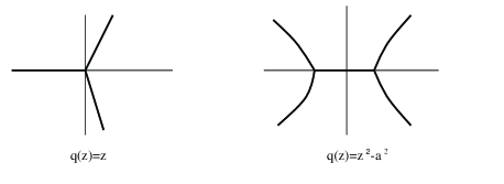
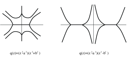
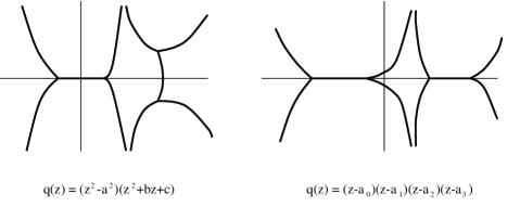
Figure 2. Stokes lines for some polynomials

Since the turning points are simple, from each turning point three Stokes lines emanate with equal angles. In general if $z_{0}$ is a turning point of order $n$, then $n+2$ Stokes lines with equal angles emanate from $z_{0}$.

2.2. Canonical Domains, Asymptotic Expansions

Since $q(z)$ is a polynomial, the Stokes graph divides the complex plane into two type of domains:

• Half-plane type: A simply connected domain $D$ which is bounded by Stokes lines is a half-plane type domain if under the map $S=S(z_{0},z)$, it is biholomorphic to a half-plane of the form $\Re S>a$ or $\Re S<a$. Here $z_{0}$ is a turning point on the boundary of $D$.

• Band-type: $D$ as above, is of band-type if under $S$, it is biholomorphic to a band of the form $a<\Re S<b$.

A domain $D$ in the complex plane is called canonical if $S(z_{0},z)$ is a one-to-one map of D onto the whole complex plane with finitely many vertical cuts such that none cross the real axis. A canonical domain is the union of two half-plane type domains and some band type domains. For example, the union of two half-plane type domains sharing a Stokes line is a canonical domain.

Let $\varepsilon>0$ be arbitrary. We denote $D^{\varepsilon}$ for the pre-image of $S(D)$ with $\varepsilon$-neighborhoods of the cuts and $\varepsilon$-neighborhoods of the turning points removed. A canonical path in $D$ is a path such that $\Re(S)$ is monotone along the path. For example, the anti-Stokes lines (lines where, $\Im(S)=0$), are canonical paths. For every point $z$ in $D^{\varepsilon}$, there are always canonical paths $\gamma^{-}(z)$ and $\gamma^{+}(z)$ from $z$ to $\infty$, such that $\Re S\downarrow-\infty$ and $\Re S\uparrow\infty$, respectively.
Now we have the following fact:

With $D$, $\gamma^{+}$, $\gamma^{-}$ as above, to within a multiple of a constant, equation (11) has a unique solution $y_{1}(z,\lambda)$, such that

(12) $$\lim_{z\to\infty,z\in\gamma^{-}}y_{1}(z,\lambda)=0,\qquad\quad\Re S(z_{0},z)\downarrow-\infty,$$

and a unique solution $y_{2}(z,\lambda)$ (up to a constant multiple), such that

(13) $$\lim_{z\to\infty,z\in\gamma{+}}y_{2}(z,\lambda)=0,\qquad\quad\Re S(z_{0},z)\uparrow\infty.$$

The solutions $y_{1}$ and $y_{2}$ in (12) and (13) have uniform asymptotic expansions in $D^{\varepsilon}$ in powers of $\frac{1}{\lambda}$. Here we only state the principle terms:

(14) $$y_{1}(z,\lambda)=q^{\frac{-1}{4}}(z)e^{\lambda S(z_{0},z)}(1+\varepsilon_{1}(z,\lambda))\qquad\lambda\to\infty,$$

(15) $$y_{2}(z,\lambda)=q^{\frac{-1}{4}}(z)e^{-\lambda S(z_{0},z)}(1+\varepsilon_{2}(z,\lambda))\qquad\lambda\to\infty,$$

where

(16) $$\varepsilon_{1}(z,\lambda)=O(\frac{1}{\lambda}),\qquad\text{uniformly in}\;D^{\varepsilon},\quad\lambda\to\infty,$$

(17) $$\varepsilon_{2}(z,\lambda)=O(\frac{1}{\lambda}),\qquad\text{uniformly in}\;D^{\varepsilon},\quad\lambda\to\infty.$$

Notice that the equalities (16) and (17) would not necessarily be uniformly in $D^{\varepsilon}$ if $q(z)$ was not a polynomial.

2.3. Elementary Basis

Let $D$ be a canonical domain, $l$ a Stokes line in $D$, and $z_{0}\in l$ a turning point. We use the triple $(D,l,z_{0})$ to denote this data. We select the branch of $S(z_{o},z)$ in $D$ such that $\Im S(z_{0},z)>0$ for $z\in l$. The elementary basis $\{u(z),v(z)\}$ associated to $(D,l,z_{0})$ is uniquely defined by

(18) $$\left\{\begin{array}[]{ll}u(z,\lambda)=cy_{1}(z,\lambda),\quad\text{and}\quad v(z,\lambda)=cy_{2}(z,\lambda),\\ \\ |c|=1,\;\text{and}\;\arg(c)=\lim_{z\to z_{0},z\in l}\arg(q^{1/4}(z)),\end{array}\right.$$

where $y_{1}(z,\lambda)$, $y_{2}(z,\lambda)$ are given by (14) and (15).

2.4. Transition Matrices

Assume $(D,l,z_{0})_{j}$ and $(D,l,z_{0})_{k}$ are two triples and $\beta_{j}=\{u_{j},v_{j}\}$ and $\beta_{k}=\{u_{k},v_{k}\}$ their corresponding elementary basis. The matrix $\Omega_{jk}(\lambda)$ which changes the basis $\beta_{j}$ to $\beta_{k}$ is called the transition matrix from $\beta_{j}$ to $\beta_{k}$.

Fedöryuk, in [EF], introduced three types of transition matrices that he called elementary transition matrices, and he proved that any transition matrix is a product of a finitely many of these elementary matrices. The three types are

• $(D,l,z_{1})\mapsto(D,l,z_{2})$. This is the transition from one turning point to another along a finite Stokes line remaining in the same canonical domain $D$. The transition matrix is given by

  (19) $$\Omega(\lambda)=e^{i\varphi}\left(\begin{array}[]{cc}0&e^{-i\lambda\alpha}\\ e^{i\lambda\alpha}&0\\ \end{array}\right),\qquad\alpha=|S(z_{1},z_{2})|,\quad e^{i\varphi}=\frac{c_{2}}{c_{1}}.$$

• $(D,l_{1},z_{1})\mapsto(D,l_{2},z_{2})$. Here the rays $S(l_{1})$ and $S(l_{2})$ are directed to one side. This is the transition from one turning point to another along an anti-Stokes line, remaining in the same domain $D$. The transition matrix is

  (20) $$\Omega(\lambda)=e^{i\varphi}\left(\begin{array}[]{cc}e^{-\lambda a}&O\\ 0&e^{\lambda a}\\ \end{array}\right),\qquad a=|S(z_{1},z_{2})|,\quad e^{i\varphi}=\frac{c_{2}}{c_{1}}.$$

• $(D_{1},l_{1},z_{0})\mapsto(D_{2},l_{2},z_{0})$ This is a simple rotation around a turning point $z_{0}$ so that $D_{1}$ and $D_{2}$ have a common sub-domain. More precisely, let $\{l_{j};j=1,2,3\}$ be the Stokes lines starting at $z_{0}$ and ordered counter-clockwise so that $l_{j+1}$ is located on the left side of $l_{j}$. We choose the canonical domain $D_{j}$ so that the part of $D_{j}$ on the left of $l_{j}$ equals the part of $D_{j+1}$ on the right of $l_{j+1}$. Then

  (21) $$\left\{\begin{array}[]{ll}\Omega_{j,j+1}(\lambda)=e^{-\frac{\pi}{6}}\left(\begin{array}[]{cc}0&\alpha_{j,j+1}^{-1}(\lambda)\\ 1&i\alpha_{j+1,j+2}(\lambda)\\ \end{array}\right),\\ \\ \alpha_{j,j+1}(\lambda)=1+O(\frac{1}{\lambda}),\quad 1\leq j\leq 3,\\ \\ \alpha_{1,2}(\lambda)\alpha_{2,3}(\lambda)\alpha_{3,1}(\lambda)=1,\quad\text{and}\quad\alpha_{j,j+1}(\lambda)\alpha_{j+1,j}(\lambda)=1.\end{array}\right.$$

2.5. Polynomials with real coefficients

We finish this section with a review of some properties of the Stokes lines and transition matrices in (21) when the polynomial $q(z)$ has real coefficients.

• The turning points and Stokes lines are symmetric about the real axis. If $x_{1}<x_{2}$ are two real turning points and $q(x)<0$ on the line segment $l=[x_{1},x_{2}]$, then $l$ is a Stokes line (See Figure 2). Similarly, if $q(x)>0$ on $l$, then $l$ is an anti-Stokes line. Let $x_{0}$ be a simple turning point on the real axis, and let $l_{0},l_{1},l_{2}$ be the Stokes lines starting at $x_{0}$. Then one of the Stokes lines, say $l_{0}$, is an interval of the real axis, and $l_{2}=\bar{l_{1}}$. The Stokes lines $l_{1}$ and $l_{2}$ do not intersect the real axis other than at the point $x_{0}$. If a Stokes line $l$ intersects the real axis at a non-turning point, then $l$ is a finite Stokes line and it is symmetric about the real axis.

  If $\lim_{x\to\infty}q(x)=\infty$, and $x^{+}$ is the the largest zero of $q(x)$, and ${l_{0},l_{1},l_{2}}$ are the corresponding Stokes lines, then there is a half type domain $D^{+}$ such that

  $$[x^{+},+\infty]\subset D^{+},\qquad D^{+}=\overline{D^{+}},\quad l_{1}\cup l_{2}\subset\partial D^{+}.$$

  Clearly $[x_{0},+\infty]$ is an anti-Stokes line and $S(x_{0},\infty)=\infty$. By (12), there exists a unique solution $y^{+}(z,\lambda)$ such that

  $$\lim_{x\to\infty}y^{+}(x,\lambda)=0.$$

  Similarly by (13) if $\lim_{x\to-\infty}q(x)=\infty$ and $x^{-}$ is the smallest root of $q(x)$, and $D^{-}$ a half type domain containing $[-\infty,x_{0}]$, there exists a unique solution $y^{-}(z,\lambda)$ such that

  $$\lim_{x\to-\infty}y^{-}(x,\lambda)=0.$$

  Therefore if $y(x,\lambda)$ is an $L^{2}$-solution to (2) , then for some constants $c^{+}$, $c^{-}$

  $$y(x,\lambda)=c^{+}y^{+}(x,\lambda)=c^{-}y^{-}(x,\lambda).$$

  Now let $\Omega_{+,-}(\lambda)$ be the transition matrix connecting $D^{+}$ to $D^{-}$ and let

  $$\left(\begin{array}[]{c}a(\lambda)\\ b(\lambda)\\ \end{array}\right)=\Omega_{+,-}(\lambda)\left(\begin{array}[]{c}0\\ 1\\ \end{array}\right).$$

  The fact that $y^{+}(x,\lambda)$ is a constant multiple of $y^{-}(x,\lambda)$ is equivalent to

  (22) $$b(\lambda)=0,$$

  which is the equation that determines the eigenvalues $\lambda_{n}$. To calculate $\Omega_{+,-}(\lambda)$ and hence $b(\lambda)$ we have to write this matrix as a product of finitely many elementary transition matrices connecting $D^{+}$ to $D^{-}$.

• When the polynomial $q(z)$ has real coefficients, the transitions matrices in (21) have some symmetries. Let $x_{0}$ be a simple turning point and $q(x)>0$ on the interval $[x_{0},b]$. We index the Stokes lines $l_{0},l_{1},l_{2}$ as in Figure (23). We define the canonical domains $D_{0},D_{1},D_{2}$ by their internal Stokes lines and their boundary Stokes lines as the following

  $$D_{0}=\overline{D_{0}},\qquad l_{0}\subset D_{0},l_{1}\cup l_{2}\subset\partial D,$$

  $$[x_{0},b]\subset D_{1},\qquad l_{0}\cup l_{2}\subset\partial D_{1},$$

  $$D_{2}=\overline{D}_{1}.$$

  

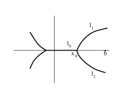
  Figure 3.

  Now with the same notation as in (21), we have

  (23) $$\alpha_{0,1}=\overline{\alpha_{0,2}},\qquad|\alpha_{1,2}|=1.$$

3. Proofs of the Theorems

First of all we have the following lemma:

Lemma 3.1.

Let $T=(D,l,z_{0})$ be a triple as in section 2.3 and let $\{u(z,\lambda),v(z,\lambda)\}$ be the elementary basis associated to $T$ in (18). We write $y(z,\lambda_{n})$ in this basis as

(24) $$y(z,\lambda_{n})=a(\lambda_{n})u(z,\lambda_{n})+b(\lambda_{n})v(z,\lambda_{n}).$$

If $\{\lambda_{n_{k}}\}$ is a subsequence of $\{\lambda_{n}\}$ such that the limit

(25) $$t=\lim_{k\to\infty}\frac{1}{2\lambda_{n_{k}}}\log|\frac{b(\lambda_{n_{k}})}{a(\lambda_{n_{k}})}|,$$

exists, then in $D^{\varepsilon}$ we have

$$Z_{\lambda_{n_{k}}}\longrightarrow\frac{1}{\pi}|\sqrt{q(z)}|\,|d\gamma|,\qquad\gamma=\{z\in D|\;\Re S(z_{0},z)=t\}.$$

The last expression means that for every $\varphi\in C_{c}^{\infty}(D^{\varepsilon})$ we have

$$Z_{\lambda_{n_{k}}}(\varphi)\to\frac{1}{\pi}\int_{\gamma}\varphi(z)|\sqrt{q(z)}||d\gamma|.$$

Proof of Lemma. For simplicity we omit the subscript $n_{k}$ in $\lambda_{n_{k}}$, but we remember that the limit in (25) is taken along $\lambda_{n_{k}}$. Using (24), (18), (14), and (15), the equation $y(z,\lambda)=0$ in $D^{\varepsilon}$, is equivalent to

(26) $$S(z_{0},z)-\frac{1}{2\lambda}\log(\frac{1+\varepsilon_{1}(z,\lambda)}{1+\varepsilon_{2}(z,\lambda)})=\frac{1}{2\lambda}\log\mid\frac{b(\lambda)}{a(\lambda)}\mid+i(\frac{2k+1}{2\lambda}\pi+\frac{1}{2\lambda}\arg(\frac{b(\lambda)}{a(\lambda)})),\qquad k\in\mathbb{Z}.$$

where we have chosen $\log z=\log r+i\theta$, $-\pi<\theta<\pi.$ We use $\tilde{S}(z)$ for the function on the left hand side of (26) and $a_{k}$ for the sequence of complex numbers on the right hand side. As we see $\tilde{S}(z)$ is the sum of the biholomorphic function $S(z_{0},z)$ and the function

(27) $$\mu(z,\lambda):=-\frac{1}{2\lambda}\log(\frac{1+\varepsilon_{1}(z,\lambda)}{1+\varepsilon_{2}(z,\lambda)})=O(\frac{1}{\lambda^{2}}),\qquad\text{uniformly in}\;D^{\varepsilon},\;\text{by}\;(\ref{ep1}),(\ref{ep2}).$$

Now suppose $\varphi\in C_{c}^{\infty}(D^{\varepsilon})$ and $K=\text{supp}(\varphi)$. We also define $K^{\prime}=S(K)$ where $S(z)=S(z_{0},z)$. Without loss of generality we can assume that $\{x=t\}\cap\text{int}(K^{\prime})$ is a connected subset of the vertical line $x=t$, because we can follow the same argument for each connected component. Now let $s=\text{length}(\{x=t\}\cap\text{int}(K^{\prime}))$. It is clear that because of (25)

(28) $$N:=\#\{\;a_{k}\in\text{int}(K^{\prime})\}\sim s\lambda.$$

We call this finite set $\{a_{k}\}_{m+1\leq k\leq m+N}$. Now let $K\subset V\subset D^{\varepsilon}$ be an open set with compact closure in $D^{\varepsilon}$. We choose $\lambda$ large enough such that

$$|\mu(z,\lambda)|<|S(z_{0},z)-a|\qquad\forall\;a\in K^{\prime},\quad\forall\;z\in\partial V.$$

Since $S$ is a biholomorphic map, by Rouché’s theorem the equation

$$\tilde{S}(z)=a_{k},\qquad m+1\leq k\leq m+N,$$

has a unique solution $z_{k}$ in $V$ for each $k$. Now by (25), (26), and (27), we have

$$z_{k}=S^{-1}\big{(}\frac{1}{2\lambda}\log\mid\frac{b(\lambda)}{a(\lambda)}\mid-\mu(z_{k},\lambda))+i(\frac{2k+1}{2\lambda}\pi+O(\frac{1}{\lambda}))\big{)}$$

$$=S^{-1}\big{(}t+o(1)+i(\frac{2k+1}{2\lambda}\pi-\Im(\mu(z_{k},\lambda))+O(\frac{1}{\lambda}))\big{)}.$$

It follows that

$$Z_{\lambda}(\varphi)=\frac{1}{\lambda}\sum_{k=m+1}^{m+N}\varphi(z_{k})=\frac{1}{\lambda}\sum_{k=m+1}^{m+N}(\varphi\circ S^{-1})\big{(}t+o(1)+i(\frac{2k+1}{2\lambda}\pi-\Im(\mu(z_{k},\lambda))+O(\frac{1}{\lambda}))\big{)}.$$

Using the mean value theorem on the $x-$axis and (28), we obtain

(29) $$\lim_{\lambda\to\infty}Z_{\lambda}(\varphi)=\lim_{\lambda\to\infty}\frac{1}{\lambda}\sum_{k=m+1}^{m+N}\{[(\varphi\circ S^{-1})\big{(}t+i\big{(}\frac{2k+1}{2\lambda}\pi-\Im(\mu(z_{k},\lambda))+O(\frac{1}{\lambda})\big{)}\big{)}]+o(1)\}.$$

Because of (27), we know that $\Im(\mu(z_{k},\lambda))=O(\frac{1}{\lambda^{2}})$ uniformly in $k$. Therefore the set

$$\wp=\{(t,\frac{2k+1}{2\lambda}\pi-\Im(\mu(z_{k},\lambda))+O(\frac{1}{\lambda}))|\;m+1\leq k\leq m+N\}$$

is a partition of the vertical interval $\{x=t\}\cap\text{int}(K^{\prime})$ with $\text{mesh}(\wp)\to 0$ as $\lambda\to\infty$. This together with (29) implies that

$$\lim_{\lambda\to\infty}Z_{\lambda}(\varphi)=\frac{1}{\pi}\int_{\{x=t\}}\varphi\circ S^{-1}dy.$$

Now, if in the last integral we apply the change of variable $z\mapsto S(z)$, then by the Cauchy-Riemann equations for $S$, we obtain

$$\frac{1}{\pi}\int_{\{x=t\}}\varphi\circ S^{-1}dy=\frac{1}{\pi}\int_{\{\Re S(z)=t\}}\varphi(z)|\sqrt{q(z)}|\,|d\gamma|.$$

This proves the Lemma.

Proof of Theorem 1.1. First of all, we cover the plane by finitely many canonical domains $D_{m}$. Let $\varepsilon>0$ be sufficiently small as before. Assume $\{Z_{\lambda_{n_{k}}}\}$ is a weak^∗ convergent subsequence converging to a measure $Z$. Clearly $\{Z_{\lambda_{n_{k}}}\}$ converges to $Z$ in each $D_{m}^{\varepsilon}$. We claim that the limit (25) exists for every triple $T_{m}=(D_{m},z_{m},l_{m})$. This is clear from Lemma 3.1. This is because if in (25) we get two distinct limits $t_{1}$ and $t_{2}$ for two subsequences of $\{Z_{\lambda_{n_{k}}}\}$, then we get two corresponding distinct limits $Z_{1}$ and $Z_{2}$ which contradicts our assumption about $\{Z_{\lambda_{n_{k}}}\}$. We should also notice that if in (25), $t=\underline{+}\infty$ then in the proof of Lemma 3.1 for $\lambda$ large enough we have $\{x=\frac{1}{2\lambda}\log\mid\frac{b(\lambda)}{a(\lambda)}\mid\}\cap\text{int}(K^{\prime})=\O$, and therefore $Z|_{D_{m}^{\varepsilon}}=0$. This means that we do not obtain any zero lines in this canonical domain. In other words the zeros run away from this canonical domain as $\lambda\to\infty$. But as we mentioned in the introduction, all the Stokes lines on the real axis are contained in the set of zero lines of every limit $Z$, meaning that in Theorem 1.1, $\gamma$ is never empty.

Now notice that because $\bigcup_{m}D_{m}^{\varepsilon}$ covers the plane except the $\varepsilon$-neighborhoods around the turning points, we have proved that

$\qquad\qquad\qquad Z(\varphi)=\frac{1}{\pi}\int_{\gamma}\varphi(z)|\sqrt{q(z)}|\,|d\gamma|,\qquad\varphi\in C_{c}^{\infty}(\mathbb{C}\backslash\bigcup_{m}B(z_{m},\varepsilon)).$

To finish the proof we have to show that if $\varphi_{\varepsilon}\in C_{c}^{\infty}(\bigcup_{m}B(z_{m},\varepsilon))$ is a bounded function of $\varepsilon$, then

$$\lim_{\varepsilon\to 0}\limsup_{\lambda_{n_{k}}\to\infty}Z_{\lambda_{n_{k}}}(\varphi_{\varepsilon})=0.$$

This is clearly equivalent to showing that if $z_{0}$ is a turning point, then

(30) $$\lim_{\varepsilon\to 0}\limsup_{\lambda\to\infty}\frac{\#\{z\in B(z_{0},\varepsilon)|\;y(z,\lambda)=0\}}{\lambda}=0.$$

To prove this we use the following fact in [F1] pages $104-105$ or [EF] pages $39-41$, which enables us to improve the domain $D^{\varepsilon}$ in (16) and (17) from a fixed $\varepsilon$ to $\varepsilon(\lambda)$ dependent of $\lambda$ such that $\varepsilon(\lambda)\to 0$ as $\lambda\to\infty$.

Let $D$ be a canonical domain with turning points $z_{m}$ on its boundary. Assume $N(\lambda)$ is a positive function such that $N(\infty)=\infty$. Now if we denote

$$D(\lambda)=D\;\backslash\bigcup_{m}B(z_{m},|q^{\prime}(z_{m})|^{-1/3}N(\lambda)\lambda^{-2/3}),$$

Then in place of equations (16) and (17) we have

$$\varepsilon_{1}(z,\lambda),\;\varepsilon_{2}(z,\lambda)=O(N(\lambda)^{-3/2}),\qquad\text{uniformly in}\;D(\lambda),\quad\lambda\to\infty.$$

In fact this implies that Lemma 3.1 is true for every $\varphi$ supported in $D$. This is because we can follow the proof of the lemma line by line except that in (27) we get $\mu(z,\lambda)=O(N(\lambda)^{-3/2}\lambda^{-1})$ uniformly in $D(\lambda)$ and therefore, using $N(\infty)=\infty$, we can still conclude $\text{mesh}(\wp)\to 0$ as $\lambda\to\infty$.

We choose $N(\lambda)=\lambda^{1/12}$. By the discussion in the last paragraph in (30) we can replace $\varepsilon$ by $\varepsilon(\lambda)=cN(\lambda)\lambda^{-2/3}=c\lambda^{-7/12}$, where $c=|q^{\prime}(z_{0})|^{-1/3}$. Let us find a bound for the number of zeros of $y(z,\lambda)$ in $B(z_{0},\varepsilon(\lambda))$. Let $M=\text{sup}_{B(z_{0},\delta)}(|q(z)|)$ where $\delta>0$ is fixed and is chosen such that the ball $B(z_{0},\delta)$ does not contain any other turning points. We also choose $\lambda$ large enough so that $\varepsilon(\lambda)<\delta$. If $\zeta$ is a zero of $y(z,\lambda)$ in the ball $B(z_{0},\varepsilon(\lambda))$ then by Corollary $11.1.1$ page $579$ of [H1] we know that there are no zeros of $y(z,\lambda)$ in the ball of radius $\frac{\pi}{\sqrt{M}}\lambda^{-1}$ around $\zeta$ except $\zeta$. Therefore

$$\#\{z\in B(z_{0},\varepsilon(\lambda))|\;y(z,\lambda)=0\}\leq\frac{\text{area}(B(z_{0},\varepsilon(\lambda)+\frac{\pi}{2\sqrt{M}}\lambda^{-1}))}{\text{area}(B(\zeta,\frac{\pi}{2\sqrt{M}}\lambda^{-1}))}=O(\lambda^{5/6}),$$

and so

$$\lim_{\lambda\to\infty}\frac{\#\{z\in B(z_{0},\varepsilon(\lambda))|\;y(z,\lambda)=0\}}{\lambda}=0.$$

This finishes the proof of Theorem 1.1.

The Proofs of Theorems 1.2, 1.4. We will not prove Theorem 1.3, because the proof is similar to (in fact easier than) the proof of the two well potential. To simplify our notations let us rename the turning points as $x_{l}=a_{0},x_{m}=a_{1},x_{n}=a_{2},x_{p}=a_{3}$. Then we can index the Stokes lines as in Fig (4).

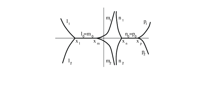
Figure 4.

We define the canonical domains $D_{l}$, $D_{m_{0}}$, $D$, $D_{n_{0}}$, and $D_{p}$ by

(31) $$\begin{array}[]{ll}l_{1}\subset D_{l},\qquad m_{1},m_{0},l_{2}\subset\partial D_{l},\\ m_{0}\subset D_{m_{0}},\qquad l_{1},l_{2},m_{1},m_{2}\subset\partial D_{m_{0}},\\ m_{1},n_{1}\subset D,\qquad l_{1},l_{0},m_{2},n_{2},p_{0},p_{1}\subset\partial D,\\ n_{0}\subset D_{n_{0}},\qquad p_{1},p_{2},n_{1},n_{2}\subset\partial D_{n_{0}},\\ p_{1}\subset D_{p},\qquad n_{1},n_{0},p_{2}\subset\partial D_{p}\;.\end{array}$$

Notice that the complex conjugates of the these canonical domains are also canonical domains and in fact if we include these complex conjugates then we obtain a covering of the plane by canonical domains. But because $q(x)$ is real, the zeros are symmetric with respect to the $x$-axis, and it is therefore enough to find the zeros in $D_{l}\cup D_{m_{0}}\cup D\cup D_{n_{0}}\cup D_{p}$. By lemma 3.1 we only need to discuss the limit (25) in each of these canonical domains. First of all let us compute the equation of the eigenvalues (22).

Here, the transition matrix $\Omega_{+,-}$, is the product of the seven elementary matrices associated to the following sequence of triples:

$(D_{p},l_{1},x_{p})\mapsto(D_{n_{0}},n_{0},x_{p})\mapsto(D_{n_{0}},n_{0},x_{n})\mapsto(D,n_{1},x_{n})$

$$\mapsto(D,m_{1},x_{m})\mapsto(D_{m_{0}},m_{0},x_{m})\mapsto(D_{m_{0}},m_{0},x_{l})\mapsto(D_{l},l_{1},x_{l}).$$

In fact if we define

$$\alpha_{1}=\int_{x_{l}}^{x_{m}}|\sqrt{q(t)}|dt,\quad\alpha_{2}=\int_{x_{n}}^{x_{p}}|\sqrt{q(t)}|dt,\quad\xi=\int_{x_{m}}^{x_{n}}\sqrt{q(t)}dt,$$

then by (19),(20) and (21), we have

$\left(\begin{array}[]{c}a(\lambda)\\ b(\lambda)\\ \end{array}\right)=\Omega_{+,-}\left(\begin{array}[]{c}0\\ 1\\ \end{array}\right)$

$$=\left(\begin{array}[]{cc}0&{\alpha_{l_{0}l_{1}}^{-1}}\\ 1&i\alpha_{l_{1}1_{2}}\\ \end{array}\right)\left(\begin{array}[]{cc}0&e^{-i\lambda\alpha_{1}}\\ e^{i\lambda\alpha_{1}}&0\\ \end{array}\right)\left(\begin{array}[]{cc}0&\alpha_{m_{1}m_{0}}^{-1}\\ 1&i\alpha_{m_{0}m_{2}}\\ \end{array}\right)\left(\begin{array}[]{cc}e^{-\lambda\xi}&0\\ 0&e^{\lambda\xi}\\ \end{array}\right)$$

$$\qquad\qquad\qquad\left(\begin{array}[]{cc}0&\alpha_{n_{0}n_{1}}^{-1}\\ 1&i\alpha_{n_{1}n_{2}}\\ \end{array}\right)\left(\begin{array}[]{cc}0&e^{-i\lambda\alpha_{2}}\\ e^{i\lambda\alpha_{2}}&0\\ \end{array}\right)\left(\begin{array}[]{cc}0&\alpha_{p_{1}p_{0}}^{-1}\\ 1&i\alpha_{p_{0}p_{2}}\\ \end{array}\right)\left(\begin{array}[]{c}0\\ 1\\ \end{array}\right).$$

A simple calculation shows that

$$b(\lambda)=\alpha_{p_{1}p_{0}}^{-1}\alpha_{n_{0}n_{1}}^{-1}e^{i\lambda(\alpha_{2}-\alpha_{1})}e^{-\lambda\xi}-(\alpha_{m_{0}m_{2}}e^{-i\lambda\alpha_{1}}+\alpha_{l_{1}l_{2}}\alpha_{m_{1}m_{0}}^{-1}e^{i\lambda\alpha_{1}})(\alpha_{p_{0}p_{2}}e^{-i\lambda\alpha_{2}}+\alpha_{n_{1}n_{2}}\alpha_{p_{1}p_{0}}^{-1}e^{i\lambda\alpha_{2}})e^{\lambda\xi}.$$

Hence $b(\lambda)=0$ implies that

(32) $$\Gamma_{1}(\lambda)\Gamma_{2}(\lambda)=\alpha_{p_{1}p_{0}}^{-1}\alpha_{n_{0}n_{1}}^{-1}e^{i\lambda(\alpha_{2}-\alpha_{1})}e^{-2\lambda\xi},$$

where

(33) $$\begin{array}[]{ll}\Gamma_{1}(\lambda)=\alpha_{m_{0}m_{2}}e^{-i\lambda\alpha_{1}}+\alpha_{l_{1}l_{2}}\alpha_{m_{1}m_{0}}^{-1}e^{i\lambda\alpha_{1}}=2\cos(\alpha_{1}\lambda)+O(\frac{1}{\lambda}),\\ \\ \Gamma_{2}(\lambda)=\alpha_{p_{0}p_{2}}e^{-i\lambda\alpha_{2}}+\alpha_{n_{1}n_{2}}\alpha_{p_{1}p_{0}}^{-1}e^{i\lambda\alpha_{2}}=2\cos(\alpha_{2}\lambda)+O(\frac{1}{\lambda}).\\ \\ \end{array}$$

Now let us discuss the limit in (25) for each of the canonical domains defined in (31). Even though the coefficients $a(\lambda)$, $b(\lambda)$ are different for different canonical domains, we do not consider it in our notation.

By (14), (15) , (16), and (17), it is clear that for $\lambda$ large enough there are no zeros in $D_{l}^{\varepsilon}$ and $D_{p}^{\varepsilon}$. For $(D_{n_{0}},n_{0},x_{p})$ we have

$$\left(\begin{array}[]{c}a(\lambda)\\ b(\lambda)\\ \end{array}\right)=\left(\begin{array}[]{cc}0&\alpha_{p_{1}p_{0}}^{-1}\\ 1&i\alpha_{p_{0}p_{2}}\\ \end{array}\right)\left(\begin{array}[]{c}0\\ 1\\ \end{array}\right)=\left(\begin{array}[]{c}\alpha_{p_{1}p_{0}}^{-1}\\ i\alpha_{p_{0}p_{2}}\\ \end{array}\right).$$

Using (21),(23), for the full sequence $\lambda_{n}$ we have

$$\frac{1}{2\lambda_{n}}\log|\frac{b(\lambda_{n})}{a(\lambda_{n})}|=\frac{1}{2\lambda_{n}}\log|\alpha_{p_{1}p_{2}}|=0.$$

Hence $t=0$ and, by Lemma 3.1, the Stokes line $n_{0}=(a_{2},a_{3})$ is a zero line in $D_{n_{0}}$. The same proof shows that the Stokes line $[a_{0},a_{1}]$ is a zero line for the full sequence $Z_{\lambda_{n}}$ in $D_{m_{0}}$. Now it only remains to discuss the limit in (25) in the canonical domain $D$. For the triple $(D,n_{1},x_{n})$ we have

$$\left(\begin{array}[]{c}a(\lambda)\\ b(\lambda)\\ \end{array}\right)=\left(\begin{array}[]{cc}0&\alpha_{n_{0}n_{1}}^{-1}\\ 1&i\alpha_{n_{1}n_{2}}\\ \end{array}\right)\left(\begin{array}[]{cc}0&e^{-i\lambda\alpha_{2}}\\ e^{i\lambda\alpha_{2}}&0\\ \end{array}\right)\left(\begin{array}[]{cc}0&\alpha_{p_{1}p_{0}}^{-1}\\ 1&i\alpha_{p_{0}p_{2}}\\ \end{array}\right)\left(\begin{array}[]{c}0\\ 1\\ \end{array}\right)=\left(\begin{array}[]{c}e^{i\lambda\alpha_{2}}\alpha_{p_{1}p_{0}}^{-1}\alpha_{n_{0}n_{1}}^{-1}\\ i\Gamma_{2}(\lambda)\\ \end{array}\right).$$

Therefore, by the second equation in (21), we obtain

(34) $$t=\lim_{n\to\infty}\frac{1}{2\lambda_{n}}\log|\frac{i\Gamma_{2}(\lambda_{n})}{e^{i\lambda_{n}\alpha_{2}}\alpha_{p_{1}p_{0}}^{-1}\alpha_{n_{0}n_{1}}^{-1}}|=\lim_{n\to\infty}\frac{1}{2\lambda_{n}}\log|\Gamma_{2}(\lambda_{n})|.$$

The limit (34) does not necessarily exist for the full sequence $\{\lambda_{n}\}$. We study this limit in different cases as follows:

1. $\frac{\alpha_{1}}{\alpha_{2}}=1$:
   

   This is exactly the symmetric case in Theorem 1.2. It is easy to see that if $\alpha_{1}=\alpha_{2}$, then there exists a translation on the real line which changes $q(z)$ to an even function. When $q(z)$ is even, because of the symmetry in the problem, we have $\Gamma_{1}(\lambda)=\Gamma_{2}(\lambda)$. On the other hand equation (32) implies that

   (35) $$|\Gamma_{1}(\lambda)||\Gamma_{2}(\lambda)|=e^{-2\lambda\xi}(1+O(\frac{1}{\lambda})).$$

   This means that in the symmetric case, the full sequence $\lambda_{n}$ satisfies

   $$|\Gamma_{1}(\lambda_{n})|=|\Gamma_{2}(\lambda_{n})|=e^{-\lambda_{n}\xi}(1+O(\frac{1}{\lambda_{n}})).$$

   Therefore, by (34) we have $t=-{\frac{1}{2}}\xi$ and using the lemma the line $\Re S(a,z)=-{\frac{1}{2}}\xi$, is the zero line in $D$. We note that this in fact determines the whole imaginary axis, because $\Re S(a,0)=-{\frac{1}{2}}\xi$. Also notice that in the symmetric case, by our notations we have $a=a_{2}=x_{n}$. This proves Theorem 1.2.2.
   

2. $\frac{\alpha_{1}}{\alpha_{2}}\neq 1$:
   

   In this case as we mentioned in the introduction, there are more than one zero limit measures. Here the limit (34) behaves differently for the two subsequences in (7) and (8) (notice that the equations (7) and (8) in fact follow from (32)). It is clear from (33) that if for a subsequence $\{\lambda_{n_{k}}\}$ we have a lower bound $\delta$ for $|\cos(\alpha_{2}\lambda_{n_{k}})|$, then we have t=$\lim_{k\to\infty}\frac{1}{2\lambda_{n_{k}}}\log|\Gamma_{2}(\lambda_{n_{k}})|=0$. Also if we have a lower bound $\delta$ for $|\cos(\alpha_{1}\lambda_{n_{k}})|$ then $\lim_{k\to\infty}\frac{1}{2\lambda_{n_{k}}}\log|\Gamma_{1}(\lambda_{n_{k}})|=0$, and by (35) we have $t=\lim_{k\to\infty}\frac{1}{2\lambda_{n_{k}}}\log|\Gamma_{2}(\lambda_{n_{k}})|=-\xi$. To find such subsequences we denote for each $\ell=1,2$

   $$A_{\delta}^{(\ell)}=\{\lambda_{n};\;|\cos(\alpha_{\ell}\lambda_{n})|>\delta\}.$$

   By (7) and (8), it is clear that up to some finite sets $A_{\delta}^{(1)}\subset\{\lambda_{n}^{(2)}\}$ and $A_{\delta}^{(2)}\subset\{\lambda_{n}^{(1)}\}$. We would like to find the density of the subsets $A_{\delta}^{(1)}$ and $A_{\delta}^{(2)}$ in $\{\lambda_{n}^{(2)}\}$ and $\{\lambda_{n}^{(1)}\}$ respectively. Here by the density of a subsequence $\{\lambda_{n_{k}}\}$ of $\{\lambda_{n}\}$ we mean

   $$d=\lim_{n\to\infty}\frac{\#\{k;\;\lambda_{n_{k}}\leq\lambda_{n}\}}{n}.$$

   If we set $\tau=\arcsin(\delta)$ then we have

   $$A_{\delta}^{(1)}=\{n\in\mathbb{N};\;|(n+{\frac{1}{2}})\frac{\alpha_{1}}{\alpha_{2}}+(m+{\frac{1}{2}})|>\tau+O(\frac{1}{n}),\quad\forall\;m\in\mathbb{Z}\},$$

   $$A_{\delta}^{(2)}=\{n\in\mathbb{N};\;|(n+{\frac{1}{2}})\frac{\alpha_{2}}{\alpha_{1}}+(m+{\frac{1}{2}})|>\tau+O(\frac{1}{n}),\quad\forall\;m\in\mathbb{Z}\}.$$

   We only discuss the density of the subset $A_{\delta}^{(1)}$. We rewrite this subset as

   $$A_{\delta}^{(1)}=\{n\in\mathbb{N};\;|(2n+1)\alpha_{1}+(2m+1)\alpha_{2}|>2\alpha_{2}\tau+O(\frac{1}{n}),\quad\forall\;m\in\mathbb{Z}\}.$$

   From this we see that if $\frac{\alpha_{1}}{\alpha_{2}}$ is a rational of the from $\frac{2r_{1}}{2r_{2}+1}$ (or $\frac{2r_{1}+1}{2r_{2}}$), then because for every $m$ and $n$ we have

   $$|(2n+1)(2r_{1})+(2m+1)(2r_{2}+1))|\geq 1,$$

   therefore $d(A_{\delta}^{(1)})=1$ for $\tau=\frac{1}{8r_{2}+4}$. This proves Theorem 1.4.2. When $\frac{\alpha_{1}}{\alpha_{2}}$ is a rational of the form $\frac{2r_{1}+1}{2r_{2}+1}$, we define

   $$B_{\delta}^{(1)}=\{n\in A_{\delta}^{(1)};\;2n+1\neq 0\;(\text{mod}\;2r_{2}+1)\}.$$

   Since for every $n\in B_{\delta}^{(1)}$ and $m\in\mathbb{Z}$ we have

   $$|(2n+1)(2r_{1}+1)+(2m+1)(2r_{2}+1))|\geq 1,$$

   for $\tau=\frac{1}{8r_{2}+4}$, we get $d(A_{\delta}^{(1)})\geq d(B_{\delta}^{(1)})=\frac{2r_{2}}{2r_{2}+1}.$ This completes the proof of Theorem 1.4.3.

   To prove Theorem 1.4.1, when $\frac{\alpha_{1}}{\alpha_{2}}$ is irrational, we use the fact that the set $\mathbb{Z}\alpha_{1}\oplus\mathbb{Z}\alpha_{2}$ is dense in $\mathbb{R}$. In fact it is easy to see that the subset $A=\{n\alpha_{1}+m\alpha_{2}|\;n\in\mathbb{N},\;m\in\mathbb{Z}\}$ is also dense. Now if we rewrite $A_{\delta}^{(1)}$ as

   $$A_{\delta}^{(1)}=\{n\in\mathbb{N};\;|(n\alpha_{1}+m\alpha_{2})+{\frac{1}{2}}(\alpha_{1}+\alpha_{2})|>\alpha_{2}\tau+O(\frac{1}{n}),\quad\forall\;m\in\mathbb{Z}\},$$

   then from the denseness of the set $A$, it is not hard to see that in this case $d(A_{\delta}^{(1)})=1-\frac{2\alpha_{2}}{\alpha_{1}}\tau.$ Hence we conclude that when $l=1$ there is a subsequence $\{\lambda_{n_{k}}^{(\ell)}\}$ of $\{\lambda_{n}^{(\ell)}\}$ of density $1$. The same argument works for $l=2$. This finishes the proof.

\begin{overpic}[scale={0.6}]{ZeroLinesDegree6.eps} \put(5.0,8.0){$q(z)=(z^{2}-a^{2})(z^{2}+bz+c)$} \put(52.0,8.0){$q(z)=(z^{2}-a^{2})(z^{2}-b^{2})(z^{2}+c^{2})$} \end{overpic}

Figure 5.

Remark 3.2.

In Figure (5) we have illustrated the zero lines for the polynomials

$$q(z)=(z^{2}-a^{2})(z^{2}+bz+c)\qquad\text{and}\qquad q(z)=(z^{2}-a^{2})(z^{2}-b^{2})(z^{2}+c^{2}).$$

The thickest lines in these figures are the zero lines. In fact for these examples there is a unique zero limit measure as in the other symmetric cases we mentioned in Theorems 1.2 and 1.3. We will not give the proofs, as they follow similarly, but we would like to ask the following question:

Is there any polynomial potential with $n$ wells, $n\geq 3$ for which there is a unique zero limit measure for the zeros of eigenfunctions?

Acknowledgements: I am sincerely grateful to Steve Zelditch for introducing the problem and many helpful discussions and suggestions on the subject.

References

- [B] Bank, S., A note on the zeros of solutions where is a polynomial, Appl. Anal. 25 (1987), no. 1-2, 29 41.
- [BS] F.A. Berezin and M.A. Shubin, The Schrodinger Equation (Moscow State University Press, Moscow 1983).
- [EF] M.A. Evgradov, M.V. Fedoryuk, Asymptotic behaviour as of the solution of the equation in the complex plane, Russian Math. Surveys, 21: 1 (1966) pp. 1 48 Uspekhi Mat. Nauk, 21: 1 (1966) pp. 3 50.
- [EGS1] A. Eremenko, A. Gabrielov, B. Shapiro, Zeros of eigenfunctions of some anharmonic oscillators, Arxiv math-ph/0612039.
- [EGS2] A. Eremenko, A. Gabrielov and Boris Shapiro, High energy eigenfunctions of one-dimensional Schrodinger operators with polynomial potentials, Arxiv math-ph/0703049.
- [F1] Fedoryuk, M. V., Asymptotic Analysis. Springer Verlag. 1993.
- [H1] E. Hille, Lectures on ordinary differential equations, Addison-Wesley, Menlo Park, CA, 1969.
- [H2] E. Hille, Ordinary differential equations in the complex domain, John Wiley and sons, NY, 1976.
- [I] E.L. Ince, Ordinary Differential Equations, Dover, New York, 1926.
- [LV] P. Leboeuf and A. Voros, Chaos-revealing multiplicative representation of quantum eigenstates, Journal of Physics A: Mathematical and General, 23 (21 May 1990) 1765-1774.
- [MGZ] Martinez-Finkelshtein A.; Martinez-Gonzalez; Zarzo A. WKB approach to zero distribution of solutions of linear second order differential equations Journal of Computational and Applied Mathematics archive Volume 1, Issue 1, August 2002.
- [MZ] A. Martinez-Finkelshtein, A. Zarzo, Zero distribution of solutions of linear second order differential equations, Complex Methods in Approximation Theory, Universidad de Almer a, 1997. Pages: 167 - 182 Year of Publication: 2002 ISSN:0377-0427.
- [N] R. Nevanlinna, Über Riemannsche Flächen mit endlich vielen Windungspunkten, Acta Math. 58, 295-373 (1932).
- [O1] FWJ Olver, Asymptotics and Special Functions, Academic Press, 1974.
- [O2] Selected papers of FWJ Olver / edited by Roderik Wong. Singapore, New Jersey, World Scientific, c2000.
- [S] Y. Sibuya, Global Theory of a Second Order Linear Ordinary Differential Equation with a Polynomial Coefficient ,North-Holland, Amsterdam, 1975.
- [SH] C. A. Swanson, V. B. Headley, An Extension of Airy’s Equation, SIAM Journal on Applied Mathematics, Vol. 15, No. 6. (Nov., 1967), pp. 1400-1412.
- [T] E. Titchmarsh, Eigenfunction expansions associated with second order differential equations, Clarendon press, Oxford, 1946.
- [W] H. Wittich, Eindeutige Lösungen der Differentialgleichung , Math. Z. 74 (1960), 278-288.
- [Z] S. Zelditch, Complex zeros of real ergodic eigenfunctions, Inventiones Mathematicae , Volume 167, Number 2, 419-443 (2007).
- [Z1] S. Zelditch, Nodal lines, ergodicity and complex numbers, The European Physical Journal-Special Topics, Volume 145, Number 1 (2007), 271-286.