Observer-based Hamiltonian identification for quantum systems

Abstract

An observer-based Hamiltonian identification algorithm for quantum systems is proposed. For the 2-level case an exponential convergence result based on averaging arguments and some relevant transformations is provided. The convergence for multi-level cases is discussed using some heuristic arguments and the relevance of the method is tested via simulations. Finally, the robustness issue with respect to non-negligible uncertainties and experimental noises is also addressed on simulations.

Keywords:

Nonlinear systems, Quantum systems, Parameter identification, Asymptotic observers, Averaging.

1 Introduction

The ability of coherent light to manipulate molecular systems at the quantum scale has been demonstrated both theoretically and experimentally [1, 16, 30, 2, 3, 24, 26, 16, 4, 31, 19, 17, 14, 23, 21, 20]. Many of the procedures, considered in this aim, are based on the possibility to perform a large number of experiments in a very small time frame. Thus, the output provided by these experiments can be used to correct the process and to identify more satisfactory control fields [8, 23, 17].

The ability to rapidly generate a large amount of quantum dynamics data may also be used to extract more information about the possibly unknown parameters of the quantum system itself. For each test field (i.e., control), there is the possibility of performing many observations for deducing information about the system, and this process can often be carried out at a much faster rate than the associated numerical simulations of the dynamics. Moreover, the recent advances in laser technology provide the means for generating a very large class of test fields for such experiments.

The rapidly developing theory of quantum parameter estimation has been investigated through different approaches. The maximum-likelihood methods and the subsequent experiment design techniques provide a first class of results in this area [18, 22, 11, 12, 13]. The optimal identification techniques via least-square criteria’s [6, 5, 15] and the map inversion techniques [27] are some other techniques explored in this area. Finally Kalman filtering techniques [7, 28] have been applied to some atomic magnetometery problems.

However, in general, developing effective identification algorithms is of a great interest in this domain. The main concerns in quantum parameter estimation theory are the presence of local minima’s for the optimization problems, sensitivity with respect to the experimental uncertainties and noises and finally the heavy cost of computations in formerly developed algorithms.

Before going through the identification and the experiment design problems, we need to ensure the identifiability of the system. This issue has been addressed in a recent work [15] where sufficient assumptions applying the uniqueness of the inversion result are provided in two relevant settings. A brief review of an identifiability result needed for the purpose of this paper is given in the Appendix A. The semi-constructive proof in [15] suggests that a well-chosen control laser field, coupling all the eigenstates of the free Hamiltonian, would be sufficient to identify the unknown parameters.

In [10], a state observer for a known quantum system is proposed. This observer is then used as a basis for the quantum parameter estimation applying an iterative search algorithm. The provided optimization algorithms typically converge toward local minima’s.

Here, in the same direction, we provide an observer-based parameter estimation algorithm based on techniques derived from adaptive control theory. In this aim, we will integrate online a generalized observer including the estimators for both the unknown state and the unknown parameters of the system.

In the next section, we will present the suggested algorithm on a simple 2-level system where the unknown parameter to identify is reduced to a real constant $\theta$ multiplying the dipole moment. After presenting the system and the estimator, we check the performance of the method by a first simulation (Subsection 2.2). Subsection 2.3 has for goal to explain the special choice of the estimator (3) and (4). Finally in Subsection 2.4, we provide a detailed proof of a convergence result.

In Section 3, we extend the observer of Section 2 to the general case of an $N$-level system. The convergence of the estimator is discussed using some formal arguments. The efficiency of the technique is then checked on two test cases of 3 and 4 dimensions.

Finally, in Section 4, we address the robustness issue with respect to the measurement and the control noises and uncertainties. The effect of different kinds of uncertainties and noises on the identification result has been checked out on simulations for the 2-level case. Similar simulations for the multi-level situations give rise to the same kind of robustness.

2 The 2-level case

2.1 The system and its estimator

In this section, we consider the 2-level system,

$$i\frac{d}{dt}\begin{pmatrix}\Psi_{1}\\ \Psi_{2}\\ \end{pmatrix}=(H+u(t)~{}\theta~{}\mu)\begin{pmatrix}\Psi_{1}\\ \Psi_{2}\\ \end{pmatrix},\qquad\Psi=\begin{pmatrix}\Psi_{1}\\ \Psi_{2}\\ \end{pmatrix}\in{\mathbb{C}}^{2}$$

$$y(t)=\left<P\Psi(t),\Psi(t)\right>,$$ (1)

$$H=\frac{\omega}{2}\sigma_{z}=\begin{pmatrix}\omega/2&0\\ 0&-\omega/2\\ \end{pmatrix},\mu=\sigma_{x}=\begin{pmatrix}0&1\\ 1&0\\ \end{pmatrix},P=(1+\sigma_{z})/2=\begin{pmatrix}1&0\\ 0&0\\ \end{pmatrix},$$

where $y$ is the system’s output, being the population of the first eigenstate of $H$. Here $\theta>0$ the dipole moment parameter is supposed to be unknown. The goal of this section is to identify this unknown parameter.

In the density matrix language, this same system can be written as,

$$\frac{d}{dt}\rho(t)=-i~{}[H+u(t)~{}\theta~{}\mu,\rho(t)],\qquad y(t)=\text{Tr}\left[P\rho(t)\right],$$ (2)

where $\rho(t)=\Psi\Psi^{\dagger}\in{\mathbb{C}}^{2\times 2}$ is the projection matrix on the wavefunction $\Psi(t)$.

We consider the laser field $u(t)$ to be in the resonant regime with respect to the natural frequency of the system (being the difference between the eigenvalues of the Hamiltonian $H$, $-\omega/2$ and $\omega/2$):

$$u(t)=A(t)\cos(\omega t),$$

where $A(t)$ is a slowly variable modulation of the amplitude. Here, for simplicity sakes, we consider a constant amplitude $A(t)\equiv A>0$.

In this paper, we propose the following observer-based parameter estimator,

$$\frac{d}{dt}\hat{\rho} =-i[H+\hat{\theta}~{}u(t)\mu,\hat{\rho}]+\Gamma(y(t)-\hat{y}(t))\left(P\hat{\rho}+\hat{\rho}P-2\text{Tr}\left[P\hat{\rho}\right]\hat{\rho}\right),$$ (3)

$$\hat{y} =\text{Tr}\left[P\hat{\rho}\right],$$

$$\frac{d}{dt}\hat{\theta} =-i\gamma~{}u(t)\text{Tr}\left[P[\mu,\hat{\rho}]\right](y(t)-\hat{y}(t)),$$ (4)

where $\gamma$ and $\Gamma$ are positive real design parameters. As we will see in Subsection 2.4, in theory, we need the following validity domain in order to ensure the convergence toward the true parameter $\theta$:

$$\Gamma\ll A\theta,\quad A\theta\ll\omega,\quad\gamma\ll\theta.$$

However, the simulations of the next subsection show that these restrictions can be much relaxed in practice. In particular, one can use instead of (3) and (4), the average estimator of Remark 1, where the high Bohr frequency is removed and that does not require the precise knowledge of the transition frequency.

2.2 Simulations

Before explaining the choice of this identification algorithm and going through the technicalities of a convergence proof, let us check the efficiency of the algorithm in a simulation.

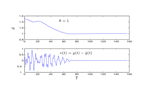
Figure 1: The first figure shows the convergence of the parameter estimator $\hat{\theta}$ towards its true value $1$; the second shows the convergence of the error term $e(t)$ toward 0.

Here, we assume the unknown parameter $\theta$, the frequency $\omega$, the constant $\Gamma$ and the laser amplitude $A$ to be all equal to 1. The constant $\gamma$ in (4) is chosen to be $\gamma=0.1$. The real system $\rho$ and the estimator $\hat{\rho}$ are respectively initialized at $\rho(0)=\Psi_{0}\Psi_{0}^{\dagger}$ and $\hat{\rho}(0)=\hat{\Psi}_{0}\hat{\Psi}_{0}^{\dagger}$ where $\Psi_{0}=(1/\sqrt{2},1/\sqrt{2})^{T}$ and $\hat{\Psi}_{0}=(1/\sqrt{5},2/\sqrt{5})^{T}$. Finally the parameter estimator $\hat{\theta}$ is initialized at $\hat{\theta}(0)=1.5$.

The simulations of Figure 1 show the result for the algorithm presented above. The simulation time $T=50\pi$ represents 25 times the natural period, at which the system without control oscillates. As it can be seen the above algorithm ensures the convergence of the parameter estimator $\hat{\theta}(t)$ toward the unknown parameter $\theta=1$.

2.3 Estimator design

In this subsection, we will explain the particular choice of the observer-based estimator (3) and (4).

Starting from the physical system (2.1), whenever the parameter $\theta$ is known, an intuitive observer (similar to the one proposed in [10]) can be given as follows:

$$\frac{d}{dt}\tilde{\Psi}=-i(H+\theta~{}u(t)\mu)\tilde{\Psi}+\Gamma(y(t)-\tilde{y}(t))P\tilde{\Psi},$$ (5)

where $\tilde{y}(t)=\left<P\tilde{\Psi}(t),\tilde{\Psi}(t)\right>$ and $\Gamma$ is a positive constant.

The non-conservative wave-functional equation (5) ($\|\tilde{\Psi}(t)\|$ does not remain constant equal to 1) can be written in the density matrix formulation as follows:

$$\frac{d}{dt}\tilde{\rho}=-i[H+\theta~{}u(t)\mu,\tilde{\rho}]+\Gamma(y(t)-\tilde{y}(t))\left(P\tilde{\rho}+\tilde{\rho}P\right),$$ (6)

where $\tilde{\rho}=\tilde{\Psi}\tilde{\Psi}^{\dagger}$ and $\tilde{y}=\text{Tr}\left[P\tilde{\rho}\right]$.

Note that unlike the conservative Schrödinger equation (2), the observer equation (6) does not conserve the trace of the density matrix $\tilde{\rho}$. However, as we will see in Subsection 2.4, enforcing the observer to keep the same geometrical structure as the main system simplifies considerably the convergence proof. In this aim we define a normalized density matrix given by $\hat{\rho}=\tilde{\rho}/\text{Tr}\left[\tilde{\rho}\right]$. This normalized observer state verifies a conservative equation of the following form

$$\frac{d}{dt}\hat{\rho}=-i[H+\theta~{}u(t)\mu,\hat{\rho}]+\Gamma(y(t)-\hat{y}(t))\left(P\hat{\rho}+\hat{\rho}P-2\text{Tr}\left[P\hat{\rho}\right]\hat{\rho}\right),$$ (7)

where $\hat{y}=\text{Tr}\left[P\hat{\rho}\right]$.

Whenever, the parameter $\theta$ is unknown, one might consider it as a part of the system’s state to be estimated. In this aim, we replace the parameter $\theta$ in (7) by $\hat{\theta}$ to be estimated (so that we obtain (3)). The question becomes now to provide an evolution equation for $\hat{\theta}$ ensuring the convergence toward the true parameter $\theta$.

Consider the Lyapunov function

$$V(t,\hat{\rho},\hat{\theta})=\frac{1}{2}(y(t)-\hat{y}(t))^{2}+\frac{1}{2\gamma}(\theta-\hat{\theta})^{2},$$ (8)

where $\gamma$ is a small enough positive constant. Deriving with respect to time, we have:

$$\frac{d}{dt}V=\left(i\hat{\theta}(t)~{}u(t)\text{Tr}\left[P[\mu,\hat{\rho}(t)]\right]-i\theta~{}u(t)\text{Tr}\left[P[\mu,\rho(t)]\right]\right)e(t)\\ +\frac{1}{\gamma}\dot{\hat{\theta}}(\hat{\theta}(t)-\theta)-2\Gamma|e(t)|^{2}\text{Tr}\left[P\hat{\rho}\right](1-\text{Tr}\left[P\hat{\rho}\right]),$$

where $e(t)=y(t)-\hat{y}(t)$. Let us take

$$\frac{d}{dt}\hat{\theta}=-i\gamma~{}u(t)\text{Tr}\left[P[\mu,\hat{\rho}]\right]e(t).$$

Then we have:

$$\frac{d}{dt}V=(i\theta~{}u(t)~{}\text{Tr}\left[P[\mu,\hat{\rho}-\rho]\right])-2\Gamma|e(t)|^{2}\text{Tr}\left[P\hat{\rho}\right](1-\text{Tr}\left[P\hat{\rho}\right]),$$ (9)

While the last term in (9) is always negative, the situation has no reason to be the same for the first one. We will see however that under certain circumstances this first term can be neglected and the Lyapunov function represents a decreasing behavior in average.

The Figure 2 illustrates the evolution of this Lyapunov function for the simulations of the last subsection.

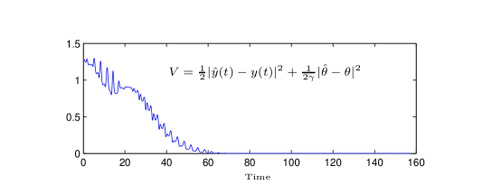
Figure 2: The positive definite function $V$ defined in (8) with $\gamma=.1$; the function decreases in average and ends up converging toward 0.

2.4 Convergence analysis

One has the following convergence result:

Theorem 1.

Consider the 2-levels system describes by

$$\left\{\begin{aligned} \frac{d}{dt}\rho(t)&=-i~{}[H+u(t)\theta\mu,\rho(t)]\\ y(t)&=\text{Tr}\left[P\rho(t)\right]\end{aligned}\right.$$ (10)

where $\rho(t)$ is the density matrix, $H=\frac{\omega}{2}\sigma_{z}$, $\mu=\sigma_{x}$, $P=(1+\sigma_{z})/2$. The goal is to estimate $\theta>0$ and $\rho$ via the measure $y$ and the knowledge of $\omega$. Assume that the estimations $\hat{\theta}$ and $\hat{\rho}$ obey the following dynamics (a nonlinear filter of $y$):

$$\left\{\begin{aligned} \frac{d}{dt}\hat{\rho}&=-i[H+\hat{\theta}~{}u(t)\mu,\hat{\rho}]+\Gamma(y(t)-\text{Tr}\left[P\hat{\rho}\right])\left(P\hat{\rho}+\hat{\rho}P-2\text{Tr}\left[P\hat{\rho}\right]\hat{\rho}\right)\\ \frac{d}{dt}\hat{\theta}&=-i\gamma~{}u(t)\text{Tr}\left[P[\mu,\hat{\rho}]\right](y(t)-\text{Tr}\left[P\hat{\rho}\right]).\end{aligned}\right.$$ (11)

where $\Gamma$ and $\gamma$ are two positive gains. Assume that $u(t)=A\cos(\omega t)$ where $A$ is a constant amplitude. Assume that the $\rho(0)$ does not belong to $\left\{\frac{1-\sigma_{x}}{2},\frac{1+\sigma_{x}}{2}\right\}$. Then exist $\epsilon>0$ and $\eta>0$, such that, for any design parameters $(A,\Gamma,\gamma)$ satisfying

$$0<\Gamma\leq\epsilon A\theta,\quad 0<A\theta\leq\epsilon\omega,\quad 0<\gamma\leq\epsilon\theta$$ (12)

and any initial conditions $(\hat{\rho}_{0},\hat{\theta}_{0})$ satisfying ($\hat{\rho}_{0}$ corresponds to a pure state, $\hat{\rho}_{0}$ is symmetric positive matrix of trace one and $\hat{\rho}^{2}_{0}=\hat{\rho}_{0}$):

$$\text{Tr}\left[(\hat{\rho}_{0}-\rho(0))^{2}\right]\leq\eta,\quad|\hat{\theta}_{0}-\theta|\leq\eta,$$

the estimates $(\hat{\rho},\hat{\theta})$ converge:

$$\lim_{t\mapsto+\infty}(\hat{\rho}(t)-\rho(t))=0,\quad\lim_{t\mapsto+\infty}\hat{\theta}(t)=\theta.$$

Moreover, this convergence is exponential (locally): it is robust to small modeling and measurements errors.

Remark 1.

The fact that $\rho(0)$ must be different from $(1\pm\sigma_{x})/2$ is not a severe limitation in practice since an alternative to (11) will be the first averaged system (13). It provides a more realistic estimator since it does not depends on $\omega$ the Bohr transition frequency that is large in general:

$$\left\{\begin{aligned} {\frac{d}{dt}}\hat{\xi}=&-i\frac{A\hat{\theta}}{2}[\sigma_{x},\hat{\xi}]+\frac{\Gamma}{4}\left(y(t)-\text{Tr}\left[\sigma_{z}\hat{\xi}\right]\right)\left(\sigma_{z}\hat{\xi}+\hat{\xi}\sigma_{z}-2\text{Tr}\left[\sigma_{z}\hat{\xi}\right]\hat{\xi}\right)\\ {\frac{d}{dt}}\hat{\theta}=&\frac{\gamma A}{4}\text{Tr}\left[\sigma_{y}\hat{\xi}\right]\left(y(t)-\text{Tr}\left[\sigma_{z}\hat{\xi}\right]\right).\end{aligned}\right.$$

More-over if the laser frequency $\omega_{r}$ does not perfectly match the resonance condition $u(t)=A\cos(\omega_{r}(t))$, the averaged estimator reads

$$\left\{\begin{aligned} {\frac{d}{dt}}\hat{\xi}=&-i\frac{\omega-\omega_{r}}{2}[\sigma_{z},\hat{\xi}]-i\frac{A\hat{\theta}}{2}[\sigma_{x},\hat{\xi}]+\frac{\Gamma}{4}\left(y(t)-\text{Tr}\left[\sigma_{z}\hat{\xi}\right]\right)\left(\sigma_{z}\hat{\xi}+\hat{\xi}\sigma_{z}-2\text{Tr}\left[\sigma_{z}\hat{\xi}\right]\hat{\xi}\right)\\ {\frac{d}{dt}}\hat{\theta}=&\frac{\gamma A}{4}\text{Tr}\left[\sigma_{y}\hat{\xi}\right]\left(y(t)-\text{Tr}\left[\sigma_{z}\hat{\xi}\right]\right).\end{aligned}\right.$$

When $|\omega-\omega_{r}|\ll A\theta$, the second averaged system is then identical to (15) and thus convergence is ensured. Thus a precise knowledge of $\omega$ is not necessary for estimating $\theta$.

Remark 2.

The simulations show that the un-normalized observer equation (5) (and the parameter estimator found by adapting this equation to the Lyapunov function (8)) would be sufficient to ensure the convergence. However, as we will see in the proof below, the trace conservation for the normalized equation simplifies considerably the analysis since $\hat{\rho}$ remains on the Bloch sphere.

The proof is based on two successive averaging: the first one relies on the resonant control $u(t)$, removes the laser frequency $\omega$ and yields to (13); the second one eliminates the Rabi frequency $A\theta$ ($A\theta\ll\omega$) and provides (15). This second averaged system is proved to be locally exponentially convergent. This implies the exponential convergence of the first averaged system (13) and of the original system (11).

Proof.

Notice first that (11) reads

$$\left\{\begin{aligned} \frac{d}{dt}\hat{\rho}&=-i\left[\frac{\omega}{2}\sigma_{z}+\hat{\theta}~{}u(t)\sigma_{x},\hat{\rho}\right]+\frac{\Gamma}{4}\text{Tr}\left[\sigma_{z}(\rho-\hat{\rho})\right]\left(\sigma_{z}\hat{\rho}+\hat{\rho}\sigma_{z}-2\text{Tr}\left[\sigma_{z}\hat{\rho}\right]\hat{\rho}\right)\\ \frac{d}{dt}\hat{\theta}&=\frac{\gamma u(t)}{2}\text{Tr}\left[\sigma_{y}\hat{\rho}\right]\text{Tr}\left[\sigma_{z}(\rho-\hat{\rho})\right].\end{aligned}\right.$$

Since $\text{Tr}\left[\hat{\rho}(0)\right]=1$ and $\text{Tr}\left[\hat{\rho}^{2}(0)\right]=1$, we have $\text{Tr}\left[\hat{\rho}(t)\right]\equiv 1$ and $\text{Tr}\left[\hat{\rho}^{2}(t)\right]\equiv 1$. Thus $\hat{\rho}$ remains a positive matrix associated to a pure state $\left|\hat{\psi}\right>\in{\mathbb{C}}^{2}$ of length one: $\hat{\rho}=\left|\hat{\psi}\right>\left<\hat{\psi}\right|$:

$$\hat{\rho}=\frac{1+\text{Tr}\left[\sigma_{x}\hat{\rho}\right]\sigma_{x}+\text{Tr}\left[\sigma_{y}\hat{\rho}\right]\sigma_{y}+\text{Tr}\left[\sigma_{z}\hat{\rho}\right]\sigma_{z}}{2}$$

where the Bloch vector of components $(\text{Tr}\left[\sigma_{x}\hat{\rho}\right],\text{Tr}\left[\sigma_{y}\hat{\rho}\right],\text{Tr}\left[\sigma_{z}\hat{\rho}\right])$ remains on the unit sphere ${\mathbb{S}}^{2}$.

The resonance assumption for the control field allows us to reduce the system by averaging and removing highly oscillating terms of frequency $\omega$. Consider the following time-dependent change of variables

$$\xi=e^{i\frac{\omega t\sigma_{z}}{2}}\rho e^{-i\frac{\omega t\sigma_{z}}{2}},\quad\hat{\xi}=e^{i\frac{\omega t\sigma_{z}}{2}}\hat{\rho}e^{-i\frac{\omega t\sigma_{z}}{2}}.$$

Since $[\sigma_{z},P]=0$, we have:

$${\frac{d}{dt}}\xi= -iA\theta\cos(\omega t)\left[e^{i\frac{\omega t\sigma_{z}}{2}}\sigma_{x}e^{-i\frac{\omega t\sigma_{z}}{2}},\xi\right]$$

$${\frac{d}{dt}}\hat{\xi}= -iA\hat{\theta}\cos(\omega t)\left[e^{i\frac{\omega t\sigma_{z}}{2}}\sigma_{x}e^{-i\frac{\omega t\sigma_{z}}{2}},\hat{\xi}\right]$$

$$\quad+\frac{\Gamma}{4}\text{Tr}\left[\sigma_{z}(\xi-\hat{\xi})\right]\left(\sigma_{z}\hat{\xi}+\hat{\xi}\sigma_{z}-2\text{Tr}\left[\sigma_{z}\hat{\xi}\right]\hat{\xi}\right)$$

$${\frac{d}{dt}}\hat{\theta}= \frac{\gamma A}{2}\cos(\omega t)\text{Tr}\left[e^{i\frac{\omega t\sigma_{z}}{2}}\sigma_{y}e^{-i\frac{\omega t\sigma_{z}}{2}}\hat{\xi}\right]\text{Tr}\left[\sigma_{z}(\xi-\hat{\xi})\right].$$

But

$$e^{i\frac{\omega t}{2}\sigma_{z}}\sigma_{x}e^{-i\frac{\omega t}{2}\sigma_{z}}=e^{i\omega t\sigma_{z}}\sigma_{x}=\cos(\omega t)\sigma_{x}-\sin(\omega t)\sigma_{y}.$$

and

$$e^{i\frac{\omega t}{2}\sigma_{z}}\sigma_{y}e^{-i\frac{\omega t}{2}\sigma_{z}}=e^{i\omega t\sigma_{z}}\sigma_{y}=\cos(\omega t)\sigma_{y}+\sin(\omega t)\sigma_{x}.$$

Take then the averaged system where the rapidly oscillating terms (associated to $\sin(2\omega t)$ or $\cos(2\omega t)$) are removed:

$$\left\{\begin{aligned} {\frac{d}{dt}}\xi=&-i\frac{A\theta}{2}[\sigma_{x},\xi]\\ {\frac{d}{dt}}\hat{\xi}=&-i\frac{A\hat{\theta}}{2}[\sigma_{x},\hat{\xi}]+\frac{\Gamma}{4}\text{Tr}\left[\sigma_{z}(\xi-\hat{\xi})\right]\left(\sigma_{z}\hat{\xi}+\hat{\xi}\sigma_{z}-2\text{Tr}\left[\sigma_{z}\hat{\xi}\right]\hat{\xi}\right)\\ {\frac{d}{dt}}\hat{\theta}=&\frac{\gamma A}{4}\text{Tr}\left[\sigma_{y}\hat{\xi}\right]\text{Tr}\left[\sigma_{z}(\xi-\hat{\xi})\right].\end{aligned}\right.$$ (13)

Consider now the new variables,

$$\zeta=e^{i\frac{A\theta t\sigma_{x}}{2}}\xi e^{-i\frac{A\theta t\sigma_{x}}{2}},\quad\hat{\zeta}=e^{i\frac{A\theta t\sigma_{x}}{2}}\hat{\xi}e^{-i\frac{A\theta t\sigma_{x}}{2}}.$$

Then (13) reads:

$${\frac{d}{dt}}\zeta =0$$ (14)

$${\frac{d}{dt}}\hat{\zeta} =-i\frac{A(\hat{\theta}-\theta)}{2}[\sigma_{x},\hat{\zeta}]$$

$$\quad+\frac{\Gamma}{4}\text{Tr}\left[e^{i\frac{A\theta t\sigma_{x}}{2}}\sigma_{z}e^{-i\frac{A\theta t\sigma_{x}}{2}}(\zeta-\hat{\zeta})\right]$$

$$\qquad\qquad\left(e^{i\frac{A\theta t\sigma_{x}}{2}}\sigma_{z}e^{-i\frac{A\theta t\sigma_{x}}{2}}\hat{\zeta}+\hat{\zeta}e^{i\frac{A\theta t\sigma_{x}}{2}}\sigma_{z}e^{-i\frac{A\theta t\sigma_{x}}{2}}-2\text{Tr}\left[e^{i\frac{A\theta t\sigma_{x}}{2}}\sigma_{z}e^{-i\frac{A\theta t\sigma_{x}}{2}}\hat{\zeta}\right]\hat{\zeta}\right)$$

$${\frac{d}{dt}}\hat{\theta} =\frac{\gamma A}{4}\text{Tr}\left[e^{i\frac{A\theta t\sigma_{x}}{2}}\sigma_{y}e^{-i\frac{A\theta t\sigma_{x}}{2}}\hat{\zeta}\right]\text{Tr}\left[e^{i\frac{A\theta t\sigma_{x}}{2}}\sigma_{z}e^{-i\frac{A\theta t\sigma_{x}}{2}}(\zeta-\hat{\zeta})\right].$$

But we have

$$e^{i\frac{A\theta t\sigma_{x}}{2}}\sigma_{y}e^{-i\frac{A\theta t\sigma_{x}}{2}}= \cos(A\theta t)\sigma_{y}-\sin(A\theta t)\sigma_{z}$$

$$e^{i\frac{A\theta t\sigma_{x}}{2}}\sigma_{z}e^{-i\frac{A\theta t\sigma_{x}}{2}}= \sin(A\theta t)\sigma_{y}+\cos(A\theta t)\sigma_{z}$$

Let us consider now the secular terms in (14), i.e., terms without the rapidly oscillating factor $\sin(2A\theta t)$ or $\cos(2A\theta t)$. The secular term in

$$\text{Tr}\left[e^{i\frac{A\theta t\sigma_{x}}{2}}\sigma_{z}e^{-i\frac{A\theta t\sigma_{x}}{2}}(\zeta-\hat{\zeta})\right]\\ \left(e^{i\frac{A\theta t\sigma_{x}}{2}}\sigma_{z}e^{-i\frac{A\theta t\sigma_{x}}{2}}\hat{\zeta}+\hat{\zeta}e^{i\frac{A\theta t\sigma_{x}}{2}}\sigma_{z}e^{-i\frac{A\theta t\sigma_{x}}{2}}-2\text{Tr}\left[e^{i\frac{A\theta t\sigma_{x}}{2}}\sigma_{z}e^{-i\frac{A\theta t\sigma_{x}}{2}}\hat{\zeta}\right]\hat{\zeta}\right)$$

is sum of two quantities

$$\frac{1}{2}\text{Tr}\left[\sigma_{y}(\zeta-\hat{\zeta})\right]\left(\sigma_{y}\hat{\zeta}+\hat{\zeta}\sigma_{y}-2\text{Tr}\left[\sigma_{y}\hat{\zeta}\right]\hat{\zeta}\right)\\ +\frac{1}{2}\text{Tr}\left[\sigma_{z}(\zeta-\hat{\zeta})\right]\left(\sigma_{z}\hat{\zeta}+\hat{\zeta}\sigma_{z}-2\text{Tr}\left[\sigma_{z}\hat{\zeta}\right]\hat{\zeta}\right)$$

The secular term for $\text{Tr}\left[e^{i\frac{A\theta t\sigma_{x}}{2}}\sigma_{y}e^{-i\frac{A\theta t\sigma_{x}}{2}}\hat{\zeta}\right]\text{Tr}\left[e^{i\frac{A\theta t\sigma_{x}}{2}}\sigma_{z}e^{-i\frac{A\theta t\sigma_{x}}{2}}(\zeta-\hat{\zeta})\right]$ is

$$\frac{1}{2}\left(\text{Tr}\left[\sigma_{y}\hat{\zeta}\right]\text{Tr}\left[\sigma_{z}(\zeta-\hat{\zeta})\right]-\text{Tr}\left[\sigma_{z}\hat{\zeta}\right]\text{Tr}\left[\sigma_{y}(\zeta-\hat{\zeta})\right]\right)$$

Thus the averaged system associated to (13) reads:

$$\left\{\begin{aligned} {\frac{d}{dt}}\zeta&=0\\ {\frac{d}{dt}}\hat{\zeta}&=-i\frac{A(\hat{\theta}-\theta)}{2}[\sigma_{x},\hat{\zeta}]\\ &\qquad+\frac{\Gamma}{8}\text{Tr}\left[\sigma_{y}(\zeta-\hat{\zeta})\right]\left(\sigma_{y}\hat{\zeta}+\hat{\zeta}\sigma_{y}-2\text{Tr}\left[\sigma_{y}\hat{\zeta}\right]\hat{\zeta}\right)\\ &\qquad+\frac{\Gamma}{8}\text{Tr}\left[\sigma_{z}(\zeta-\hat{\zeta})\right]\left(\sigma_{z}\hat{\zeta}+\hat{\zeta}\sigma_{z}-2\text{Tr}\left[\sigma_{z}\hat{\zeta}\right]\hat{\zeta}\right)\\ {\frac{d}{dt}}\hat{\theta}&=\frac{\gamma A}{8}\left(\text{Tr}\left[\sigma_{y}\hat{\zeta}\right]\text{Tr}\left[\sigma_{z}(\zeta-\hat{\zeta})\right]-\text{Tr}\left[\sigma_{z}\hat{\zeta}\right]\text{Tr}\left[\sigma_{y}(\zeta-\hat{\zeta})\right]\right).\end{aligned}\right.$$ (15)

Consider now the following Lyapounov function:

$$V(\hat{\zeta},\hat{\theta})=\frac{1}{2}\text{Tr}\left[\sigma_{y}(\hat{\zeta}-\zeta)\right]^{2}+\frac{1}{2}\text{Tr}\left[\sigma_{z}(\hat{\zeta}-\zeta)\right]^{2}+\frac{4}{\gamma}(\hat{\theta}-\theta)^{2}.$$

One has

$$\frac{4}{\Gamma}{\frac{d}{dt}}V=\left(\text{Tr}\left[\sigma_{y}(\hat{\zeta}-\zeta)\right]\text{Tr}\left[\sigma_{y}\hat{\zeta}\right]+\text{Tr}\left[\sigma_{z}(\hat{\zeta}-\zeta)\right]\text{Tr}\left[\sigma_{z}\hat{\zeta}\right]\right)^{2}\\ -\text{Tr}\left[\sigma_{y}(\hat{\zeta}-\zeta)\right]^{2}-\text{Tr}\left[\sigma_{z}(\hat{\zeta}-\zeta)\right]^{2}.$$

We have (Cauchy-Schwartz inequality)

$$\frac{4}{\Gamma}{\frac{d}{dt}}V\leq\left(\text{Tr}\left[\sigma_{y}\hat{\zeta}\right]^{2}+\text{Tr}\left[\sigma_{z}\hat{\zeta}\right]^{2}-1\right)\left(\text{Tr}\left[\sigma_{y}(\hat{\zeta}-\zeta)\right]^{2}+\text{Tr}\left[\sigma_{z}(\hat{\zeta}-\zeta)\right]^{2}\right)$$

Since $\text{Tr}\left[\sigma_{y}\hat{\zeta}\right]^{2}+\text{Tr}\left[\sigma_{z}\hat{\zeta}\right]^{2}\leq 1$, ${\frac{d}{dt}}V\leq 0$. When ${\frac{d}{dt}}V=0$ we have

• either

  $$\text{Tr}\left[\sigma_{y}(\hat{\zeta}-\zeta)\right]^{2}+\text{Tr}\left[\sigma_{z}(\hat{\zeta}-\zeta)\right]^{2}=0.$$

  This means that $\text{Tr}\left[\sigma_{x}\hat{\zeta}\right]=\pm\text{Tr}\left[\sigma_{x}\zeta\right]$:

  $$\hat{\zeta}=\zeta_{\pm}=\frac{I\pm\text{Tr}\left[\sigma_{x}\zeta\right]\sigma_{x}+\text{Tr}\left[\sigma_{y}\zeta\right]\sigma_{y}+\text{Tr}\left[\sigma_{z}\zeta\right]\sigma_{z}}{2}.$$

  We can use here Lasalle invariance principle since $\hat{\zeta}$ evolves on a compact manifold and $V$ is infinite when $\hat{\theta}$ is infinite. Since $\hat{\zeta}$ is constant, we have ${\frac{d}{dt}}\hat{\zeta}=0$ and thus $(\hat{\theta}-\theta)[\sigma_{x},\zeta]=0$. Since $\rho(0)\neq(1\pm\sigma_{x})/2$, $\zeta(t)=\zeta(0)\approx\rho(0)\neq(1\pm\sigma_{x})/2$ and thus $[\sigma_{x},\zeta]\neq 0$. This implies that $\hat{\theta}=\theta$. A simple inspection shows that $(\zeta_{-},\theta)$ is an unstable equilibria for $(\hat{\zeta},\hat{\theta})$ and $(\zeta_{+}=\zeta,\theta)$ is an asymptotically and exponentially stable one (use on the first order approximation the same Lyapounov function and the invariance principle that proves the asymptotic stability of the first variation, and thus its exponentially stability).

• or (equality case for the Cauchy-Schwartz inequality)

  $$\text{Tr}\left[\sigma_{y}\hat{\zeta}\right]=\alpha\text{Tr}\left[\sigma_{y}\zeta\right],\quad\text{Tr}\left[\sigma_{z}\hat{\zeta}\right]=\alpha\text{Tr}\left[\sigma_{z}\zeta\right],$$

  for some real $\alpha$ and

  $$\text{Tr}\left[\sigma_{y}\hat{\zeta}\right]^{2}+\text{Tr}\left[\sigma_{z}\hat{\zeta}\right]^{2}=1.$$

  Thus we have

  $$\hat{\zeta}=\zeta_{\pm}=\frac{I\pm\left(\frac{\text{Tr}\left[\sigma_{y}\zeta\right]}{\sqrt{\text{Tr}\left[\sigma_{y}\zeta\right]^{2}+\text{Tr}\left[\sigma_{z}\zeta\right]^{2}}}\sigma_{y}+\frac{\text{Tr}\left[\sigma_{z}\zeta\right]}{\sqrt{\text{Tr}\left[\sigma_{y}\zeta\right]^{2}+\text{Tr}\left[\sigma_{z}\zeta\right]^{2}}}\sigma_{z}\right)}{2}.$$

  Moreover using LaSalle invariance principle and developing $d\hat{\zeta}/dt=0$, we obtain $\hat{\theta}=\theta$. One can easily see that $(\hat{\zeta}=\zeta_{\pm},\hat{\theta}=\theta)$ are also equilibrium points of the system.

  However, note that we are looking for a local result. For initial state $(\hat{\zeta}_{0},\hat{\theta}_{0})$ near enough to the initial state $(\zeta,\theta)$, we have

  $$V(\hat{\zeta}_{0},\hat{\theta}_{0})<\epsilon\ll 1.$$

  As the Lyapunov function $V$ keeps decreasing and by choosing $\epsilon$ to be small enough ($\epsilon<\frac{1}{2}\left(1+\sqrt{\text{Tr}\left[\sigma_{y}\zeta\right]^{2}+\text{Tr}\left[\sigma_{z}\zeta\right]^{2}}\right)^{2}$), the state $(\hat{\zeta},\hat{\theta})$ can not reach the equilibrium states $(\zeta_{-},\theta)$ where we have:

  $$V(\zeta_{-},\theta)=\frac{1}{2}\left(1+\sqrt{\text{Tr}\left[\sigma_{y}\zeta\right]^{2}+\text{Tr}\left[\sigma_{z}\zeta\right]^{2}}\right)^{2}>\epsilon.$$

  Concerning the equilibria $(\zeta_{+},\theta)$, we still have two situations:

  1. either $\text{Tr}\left[\sigma_{x}\zeta\right]=0$, in which case $\zeta_{+}=\zeta$ and we have the convergence as we wanted to prove in the theorem.

  2. or $\text{Tr}\left[\sigma_{x}\zeta\right]\neq 0$ which implies that $\sqrt{\text{Tr}\left[\sigma_{y}\zeta\right]^{2}+\text{Tr}\left[\sigma_{z}\zeta\right]^{2}}<1$. In this case we choose

     $$V(\hat{\zeta}_{0},\hat{\theta}_{0})<\epsilon\ll 1,$$

     with $0<\epsilon<\frac{1}{2}\left(1-\sqrt{\text{Tr}\left[\sigma_{y}\zeta\right]^{2}+\text{Tr}\left[\sigma_{z}\zeta\right]^{2}}\right)^{2}$. As the Lyapunov function $V$ keeps decreasing, the state $(\hat{\zeta},\hat{\theta})$ can not reach the equilibrium states $(\zeta_{+},\theta)$ where we have:

     $$V(\zeta_{+},\theta)=\frac{1}{2}\left(1-\sqrt{\text{Tr}\left[\sigma_{y}\zeta\right]^{2}+\text{Tr}\left[\sigma_{z}\zeta\right]^{2}}\right)^{2}>\epsilon.$$

This asymptotic analysis based on the above Lyapounov function and Lasalle invariance principle shows that the steady-state $(\hat{\zeta},\hat{\theta})=(\zeta,\theta)$ of the average system (15) is locally exponentially stable.

The existence of $\epsilon$ and $\eta$ results from a classical lemma concerning the averaging techniques (cf. [9], Page 333, Theorem 8.3): if the average system admits an exponentially stable steady-state that is also an equilibrium of the original system, then this steady-state is also exponentially stable for the original system.

Consider first (15):

• It admits $(\zeta,\theta)$ as exponentially stable steady-state.

• it corresponds to the averaging of (14) when $A\theta\gg\Gamma,\gamma A$.

Thus the state $(\hat{\zeta},\hat{\theta})$ of (14) converge exponentially towards $(\zeta,\theta)$. Since

$$\hat{\xi}=e^{-i\frac{A\theta t\sigma_{x}}{2}}\hat{\xi}e^{+i\frac{A\theta t\sigma_{x}}{2}},\quad\xi=e^{-i\frac{A\theta t\sigma_{x}}{2}}\xi e^{+i\frac{A\theta t\sigma_{x}}{2}}$$

$\hat{\xi}-\xi$ and $\hat{\theta}-\theta$ converge exponentially towards $0$. when $\omega\gg A\theta$, a similar argument between (11) and (13) yields to the local exponential convergence of $\hat{\rho}-\rho$ and $\hat{\theta}-\theta$ towards $0$.

∎

Remark 3.

Theorem 1 provides a local convergence result for the estimator equations given by (11). The simulations, however, show a much stronger global convergence behavior. Notice that we cannot prove directly that (13) is stable, although the following function

$$V(\hat{\xi}-\xi,\hat{\theta}-\theta)=\frac{1}{2}\text{Tr}\left[\sigma_{x}(\hat{\xi}-\xi)\right]^{2}+\frac{2}{\gamma}(\hat{\theta}-\theta)^{2}$$

is decreasing in average since

$${\frac{d}{dt}}V=-\frac{\Gamma}{2}\text{Tr}\left[\sigma_{z}(\hat{\xi}-\xi)\right]^{2}\left(1-\text{Tr}\left[\sigma_{z}\hat{\xi}\right]^{2}\right)+A\theta\text{Tr}\left[\sigma_{y}(\hat{\xi}-\xi)\right].$$

The first term of the left hand side is always negative whereas the second one admits a zero average. Thus in average, $V$ is a decreasing function of time.

3 The general case

In this section, we extend the above identification algorithm to the general case of a multi-level system. Before going through this extension, we need to address the non-trivial identifiability problem for the multi-level case. The Appendix A (based on the result of [15]) provides sufficient assumptions ensuring the identifiability.

3.1 Formal extension

Consider the $N$-levels system, $(\left|j\right>)_{1\leq j\leq N}$, described by the density matrix $\rho$ that obey the following dynamics (we assume here the assumptions A1,A2 and A3 of the Appendix A to be satisfied):

$$\left\{\begin{aligned} \frac{d}{dt}\rho&=-i[H+u(t)\mu,\rho]\end{aligned}\right.$$ (16)

where

• $H=\sum_{j=1}^{N}\omega_{j}\left|j\right>\left<j\right|$ is the free Hamiltonian with $\omega_{j}$ real and satisfying $|\omega_{l}-\omega_{k}|\neq|\omega_{l^{\prime}}-\omega_{k^{\prime}}|$ for any distinct couples $(l,k)$ and $(l^{\prime},k^{\prime})$.

• $\mu=\sum_{1\leq l<k\leq N}\theta_{lk}\left(\left|k\right>\left<l\right|+\left|l\right>\left<k\right|\right)$ where $\theta_{lk}$ are the parameters to identify

• the electromagnetic field is represented by the scalar input $u(t)\in{\mathbb{R}}$

We assume that

$$y_{j}(t)=\text{Tr}\left[P_{j}\rho(t)\right],\quad P_{j}=\left|j\right>\left<j\right|,\quad j=1,2,...,N$$

are the measured outputs. The goal is to estimate the coefficient $\theta_{lk}$. The $\omega_{j}$ are known.

The estimator (11) admits then the following generalization $(1\leq l<k\leq N)$:

$$\left\{\begin{aligned} {\frac{d}{dt}}\hat{\rho}&=-i[H+u(t)\hat{\mu},\hat{\rho}]+\Gamma\sum_{j=1}^{N}\left(y_{j}(t)-\text{Tr}\left[P_{j}\hat{\rho}\right]\right)\left(P_{j}\hat{\rho}+\hat{\rho}P_{j}-2\text{Tr}\left[P_{j}\hat{\rho}\right]\hat{\rho}\right)\\ {\frac{d}{dt}}\hat{\theta}_{lk}&=-i\gamma_{lk}~{}u(t)\sum_{j=1}^{N}\text{Tr}\left[P_{j}\left[\left|l\right>\left<k\right|+\left|k\right>\left<l\right|,\hat{\rho}\right]\right]\left(y_{j}(t)-\text{Tr}\left[P_{j}\hat{\rho}\right]\right)\end{aligned}\right.$$ (17)

where $\hat{\mu}=\sum_{1\leq l<k\leq N}\hat{\theta}_{lk}\left(\left|l\right>\left<k\right|+\left|k\right>\left<l\right|\right)$, $\Gamma>0$ and $\gamma_{lk}>0$ are design parameters. Notice that $\hat{\rho}$ remains a projector if its initial condition is also a projector.

Set $u(t)=\sum_{1\leq l<k\leq N}A_{lk}\cos(\omega_{lk}t)$ where $\omega_{lk}=\omega_{l}-\omega_{k}$ and $A_{lk}$ is a constant amplitude. Let us compute, at least formally, the averaged system associated to (17) when

$$0<\Gamma\ll A_{lk}\theta_{lk}\ll\omega_{lk},\quad\gamma_{lk}\ll\theta_{lk}.$$

Consider the ”Pauli matrices” associated to the transition between $l$ and $k$:

$$\sigma_{x}^{lk}=\left|l\right>\left<k\right|+\left|k\right>\left<l\right|,\quad\sigma_{y}^{lk}=-i\left|l\right>\left<k\right|+i\left|k\right>\left<l\right|$$

$$\sigma_{z}^{lk}=P_{l}-P_{k}=\left|l\right>\left<l\right|-\left|k\right>\left<k\right|,\quad I^{lk}=P_{l}+P_{k}=\left|l\right>\left<l\right|+\left|k\right>\left<k\right|$$

For each $l\neq k$, we have the usual relations:

$$(\sigma_{x}^{lk})^{2}=I^{lk},\quad\sigma_{x}^{lk}\sigma_{y}^{lk}=i\sigma_{z}^{lk},\quad\ldots$$

For each $j$ and $k\neq j$, $P_{j}=\frac{I^{jk}+\sigma_{z}^{jk}}{2}$. In the sequel, we use the shortcut notation $\sum_{lk}$ that stands for $\sum_{1\leq l<k\leq N}$. Thus we have

$$u=\sum_{lk}A_{lk}\cos(\omega_{lk}t),\quad\mu=\sum_{lk}\theta_{lk}\sigma_{x}^{lk}.$$

Notice that when $j\neq l$ and $j\neq k$, $\text{Tr}\left[P_{j}[\sigma_{x}^{lk},\hat{\rho}]\right]\equiv 0$. When $j=l$, set $P_{l}=(I^{lk}+\sigma_{z}^{lk})/2$ to find

$$\text{Tr}\left[P_{l}[\sigma_{x}^{lk},\hat{\rho}]\right]=i\text{Tr}\left[\sigma_{y}^{lk}\hat{\rho}\right]$$

When $j=k$ we have similarly

$$\text{Tr}\left[P_{k}[\sigma_{x}^{lk},\hat{\rho}]\right]=-i\text{Tr}\left[\sigma_{y}^{lk}\hat{\rho}\right].$$

Thus (17) reads (remember that $P_{l}-P_{k}=\sigma_{z}^{lk}$).

$${\frac{d}{dt}}\hat{\rho} =-i[H,\hat{\rho}]-i\sum_{lk}\sum_{l^{\prime}k^{\prime}}A_{l^{\prime}k^{\prime}}\hat{\theta}_{lk}\cos(\omega_{l^{\prime}k^{\prime}}t)[\sigma_{x}^{lk},\hat{\rho}]$$

$$\qquad+\Gamma\sum_{j=1}^{N}\text{Tr}\left[P_{j}(\rho-\hat{\rho})\right]\left(P_{j}\hat{\rho}+\hat{\rho}P_{j}-2\text{Tr}\left[P_{j}\hat{\rho}\right]\hat{\rho}\right)$$

$${\frac{d}{dt}}\hat{\theta}_{lk} =\gamma_{lk}\left(\sum_{l^{\prime}k^{\prime}}A_{l^{\prime}k^{\prime}}\cos(\omega_{l^{\prime}k^{\prime}}t)\right)\text{Tr}\left[\sigma_{y}^{lk}\hat{\rho}\right](\text{Tr}\left[\sigma_{z}^{lk}(\rho-\hat{\rho})\right])$$

In the inter-action frame, $\xi=e^{iHt}\rho e^{-iHt}$ and $\hat{\xi}=e^{iHt}\hat{\rho}e^{-iHt}$, we have

$${\frac{d}{dt}}\hat{\xi} =-i\sum_{lk}\sum_{l^{\prime}k^{\prime}}A_{l^{\prime}k^{\prime}}\hat{\theta}_{lk}\cos(\omega_{l^{\prime}k^{\prime}}t)\left[e^{iHt}\sigma_{x}^{lk}e^{-iHt},\hat{\xi}\right]$$

$$\qquad+\Gamma\sum_{j=1}^{N}\text{Tr}\left[P_{j}(\xi-\hat{\xi})\right]\left(P_{j}\hat{\xi}+\hat{\xi}P_{j}-2\text{Tr}\left[P_{j}\hat{\xi}\right]\hat{\xi}\right)$$

$${\frac{d}{dt}}\hat{\theta}_{lk} =\gamma_{lk}\left(\sum_{l^{\prime}k^{\prime}}A_{l^{\prime}k^{\prime}}\cos(\omega_{l^{\prime}k^{\prime}}t)\right)\text{Tr}\left[e^{iHt}\sigma_{y}^{lk}e^{-iHt}\hat{\xi}\right]\text{Tr}\left[\sigma_{z}^{lk}(\xi-\hat{\xi})\right]$$

since $[P_{j},H]=0$. Simple computations show

$$e^{iHt}\sigma_{x}^{lk}e^{-iHt}=e^{i\omega_{lk}t\sigma_{z}^{lk}}\sigma_{x}^{lk}=\cos(\omega_{lk}t)\sigma_{x}^{lk}-\sin(\omega_{lk}t)\sigma_{y}^{lk}$$

and

$$e^{iHt}\sigma_{y}^{lk}e^{-iHt}=e^{i\omega_{lk}t\sigma_{z}^{lk}}\sigma_{y}^{lk}=\sin(\omega_{lk}t)\sigma_{x}^{lk}+\cos(\omega_{lk}t)\sigma_{y}^{lk}$$

For $(l,k)\neq(l^{\prime},k^{\prime})$, $|\omega_{lk}|\neq|\omega_{l^{\prime}k^{\prime}}|$. Thus resonant terms come only from $(l,k)=(l^{\prime},k^{\prime})$. The ”rotating wave approximation” of (17) reads:

$$\left\{\begin{aligned} {\frac{d}{dt}}\hat{\xi}=&-i\sum_{lk}\frac{A_{lk}\hat{\theta}_{lk}}{2}\left[\sigma_{x}^{lk},\hat{\xi}\right]\\ &+\Gamma\sum_{j=1}^{N}\text{Tr}\left[P_{j}(\xi-\hat{\xi})\right]\left(P_{j}\hat{\xi}+\hat{\xi}P_{j}-2\text{Tr}\left[P_{j}\hat{\xi}\right]\hat{\xi}\right)\\ {\frac{d}{dt}}\hat{\theta}_{lk}=&\frac{\gamma_{lk}A_{lk}}{2}\text{Tr}\left[\sigma_{y}^{lk}\hat{\xi}\right]\text{Tr}\left[\sigma_{z}^{lk}(\xi-\hat{\xi})\right]\end{aligned}\right.$$ (18)

Notice that, instead of using (17) as estimator, one can use in practice such averaged filter where the large transition frequencies $\omega_{lk}$ are removed:

$$\left\{\begin{aligned} {\frac{d}{dt}}\hat{\xi}=&-i\sum_{lk}\frac{A_{lk}\hat{\theta}_{lk}}{2}\left[\sigma_{x}^{lk},\hat{\xi}\right]\\ &+\Gamma\sum_{j=1}^{N}\left(y_{j}(t)-\text{Tr}\left[P_{j}\hat{\xi}\right]\right)\left(P_{j}\hat{\xi}+\hat{\xi}P_{j}-2\text{Tr}\left[P_{j}\hat{\xi}\right]\hat{\xi}\right)\\ {\frac{d}{dt}}\hat{\theta}_{lk}=&\frac{\gamma_{lk}A_{lk}}{2}\text{Tr}\left[\sigma_{y}^{lk}\hat{\xi}\right]\left(y_{l}(t)-y_{k}(t)-\text{Tr}\left[\sigma_{z}^{lk}\hat{\xi}\right]\right).\end{aligned}\right.$$ (19)

Let us now generalize the heuristic argument of remark 3 for the stability of (13). Consider the following function

$$V=\frac{1}{2}\sum_{n=1}^{N}\text{Tr}\left[P_{n}(\hat{\xi}-\xi)\right]^{2}+\sum_{lk}\frac{2(\hat{\theta}_{lk}-\theta_{lk})^{2}}{\gamma_{lk}}.$$ (20)

One can easily see that

$$\frac{dV}{dt}=\sum_{lk}\frac{A_{lk}\theta_{lk}}{2}\text{Tr}\left[\sigma_{z}^{lk}(\xi-\hat{\xi})\right]\text{Tr}\left[\sigma_{y}^{lk}(\xi-\hat{\xi})\right]\\ -2\Gamma\sum_{l}\sum_{k<l}\text{Tr}\left[P_{k}\hat{\xi}\right]\text{Tr}\left[P_{l}\hat{\xi}\right]\text{Tr}\left[\sigma_{z}^{kl}(\xi-\hat{\xi})\right]^{2}.$$ (21)

While the second term in (21) is obviously negative, the first term has no reason to be negative. However, we will show by a formal argument that (considering some appropriate assumption concerning the Rabi frequencies) this term can be averaged to zero and thus can be neglected.

In this aim, consider the real effective Hamitonian:

$$H_{eff}=\sum_{lk}\frac{A_{lk}\theta_{lk}}{2}\sigma_{x}^{lk},$$

and diagonalize it as follows:

$$H_{eff}=E^{\dagger}\Omega E,\qquad\Omega=diag(\Omega_{1},...,\Omega_{N}),\qquad E_{lk}\in{\mathbb{R}}\quad\forall l,k.$$

where $\{\Omega_{j}\}_{j=1}^{N}$ are Rabi frequencies of the system. From now on, we will assume that these Rabi frequencies are non-degenerate ($\Omega_{m}\neq\Omega_{n}$ for $m\neq n$) and moreover that $\Gamma\ll\Delta_{\Omega}$ and $\gamma_{l}k\ll\Delta_{\Omega}$, where $\Delta_{\Omega}=\max_{m\neq n}|\Omega_{m}-\Omega_{n}|$.

Now, in analogy with the 2-level case, consider the unitary transformation

$$\zeta=U^{\dagger}E\xi E^{\dagger}U,\quad\hat{\zeta}=U^{\dagger}E\hat{\xi}E^{\dagger}U,$$

where $U(t)=\exp(-it\Omega)$. Under such a transformation $\zeta$ is trivially constant $\zeta=E\xi_{0}E^{\dagger}$. Furthermore, this transformation also removes the highly oscillating part of $\hat{\xi}$, ($|\hat{\theta}_{lk}-\theta_{lk}|\ll\theta_{mn}$ and $\Gamma\ll A_{lk}\theta_{lk}$ for all $l,k,m,n$):

$${\frac{d}{dt}}\hat{\zeta}=-i\sum_{lk}\frac{A_{lk}(\hat{\theta}_{lk}-\theta_{lk})}{2}\left[U^{\dagger}E\sigma_{x}^{lk}E^{\dagger}U,\hat{\zeta}\right]\\ +\Gamma\sum_{j=1}^{N}\text{Tr}\left[U^{\dagger}EP_{j}E^{\dagger}U(\zeta-\hat{\zeta})\right]\left(U^{\dagger}EP_{j}E^{\dagger}U\hat{\zeta}+\hat{\zeta}U^{\dagger}EP_{j}E^{\dagger}U-2\text{Tr}\left[U^{\dagger}EP_{j}E^{\dagger}U\hat{\zeta}\right]\hat{\zeta}\right).$$

Now let us develop the terms in the first part of (21) using this unitary transformation:

$$\text{Tr}\left[\sigma_{z}^{lk}(\xi-\hat{\xi})\right]\text{Tr}\left[\sigma_{y}^{lk}(\xi-\hat{\xi})\right]=$$

$$\text{Tr}\left[U^{\dagger}E\sigma_{z}^{lk}E^{\dagger}U(\zeta-\hat{\zeta})\right]\text{Tr}\left[U^{\dagger}E\sigma_{y}^{lk}E^{\dagger}U(\zeta-\hat{\zeta})\right]=$$

$$i\left(\sum_{r\neq s}\exp(i(\Omega_{r}-\Omega_{s})t)(E_{rl}E_{sl}-E_{rk}E_{sk})(\zeta_{sr}-\hat{\zeta}_{sr})+\sum_{r}(E_{rl}^{2}-E_{rk}^{2})(\zeta_{rr}-\hat{\zeta}_{rr})\right)$$

$$\qquad\qquad\qquad\qquad\left(\sum_{r\neq s}\exp(i(\Omega_{r}-\Omega_{s})t)(E_{rl}E_{sk}-E_{rk}E_{sl})(\zeta_{sr}-\hat{\zeta}_{sr})\right).$$

Developing and removing the highly oscillating terms of frequencies $\Delta_{\Omega}$, we find

$$\sum_{r\neq s} (E_{rl}E_{sl}-E_{rk}E_{sk})(E_{rk}E_{sl}-E_{rl}E_{sk})|\zeta_{sr}-\hat{\zeta}_{sr}|^{2}=$$

$$\frac{1}{2}\sum_{r\neq s}((E_{rl}E_{sl}-E_{rk}E_{sk})(E_{rl}E_{sk}-E_{rk}E_{sl})|\zeta_{rs}-\hat{\zeta}_{rs}|^{2}+$$

$$\qquad\qquad(E_{rl}E_{sl}-E_{rk}E_{sk})(E_{sl}E_{rk}-E_{sk}E_{rl})|\zeta_{sr}-\hat{\zeta}_{sr})^{2}|=0,$$

where we have broken the sum into two parts by symmetrizing with respect to the indices $r$ and $s$.

Even though this argument does not prove the convergence of the estimator for the multi-level system, it gives a strong reason for it to be efficient. The simulations of the next section show that this is effectively the case.

3.2 Simulations

Let us check out the performance of this algorithm on two other test cases: first on a 3-level system and next on the 4-level system also considered in [15].

The first test case is given by

$$H=\begin{pmatrix}0&0&0\\ 0&1&0\\ 0&0&3\\ \end{pmatrix}\qquad\text{and}\qquad\mu=\begin{pmatrix}0&1.3&1\\ 1.3&0&-1.5\\ 1&-1.5&0\\ \end{pmatrix}.$$

We consider a laser field resonant with all the transition frequencies of the system:

$$u(t)=A~{}\left(\sin(t)+\sin(2t)+\sin(3t)\right),$$

where the laser amplitude $A$ here is chosen to be $0.1$. This allows us to use the rotating wave approximation (averaging) and eliminate the Hamiltonian $H_{0}$ in order to obtain an effective Hamiltonian $H_{eff}$.

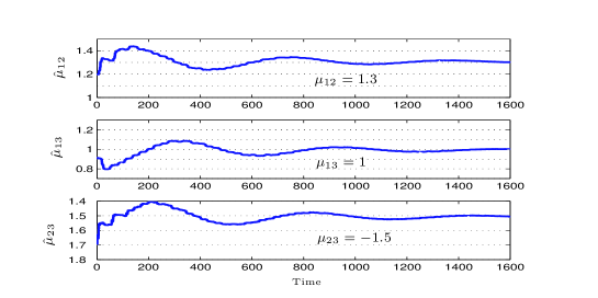
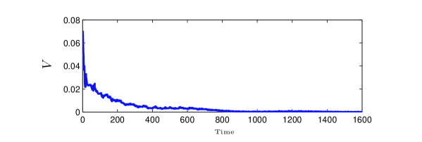
Figure 3: This figure illustrates the evolution of the estimator $\hat{\mu}$; the estimator gives a very good approximation of the real dipole moment $\mu$.

Figure 4: The positive definite function $V$ defined in (20) with $\gamma_{lk}=.5$; the function decreases in average and ends up converging toward 0.

The Figures 4 and 4 illustrate the simulations of the filter equation (17) where the following constants have been used: $\gamma=1$, $\Gamma=.05$, $A=0.1$. The simulation time $T=1600$ represents around 250 times the largest period of the system’s Hamiltonian $H$. This, however, represents only about 25 times the largest period of the effective Hamiltonian $H_{eff}$. Furthermore, the parameter estimator $\hat{\mu}$, the state estimator $\hat{\rho}=\hat{\Psi}\hat{\Psi}^{\dagger}$ and the real state $\rho=\Psi\Psi^{\dagger}$ are initialized at:

$$\hat{\mu}(0)=\begin{pmatrix}0&1.2&.9\\ 1.2&0&-1.7\\ .9&-1.7&0\\ \end{pmatrix}\quad,\quad\hat{\Psi}(0)=\begin{pmatrix}1/\sqrt{14}\\ 2/\sqrt{14}\\ 3/\sqrt{14}\\ \end{pmatrix}\quad,\quad\Psi(0)=\begin{pmatrix}1/\sqrt{30}\\ 2/\sqrt{30}\\ 5/\sqrt{30}\\ \end{pmatrix}.$$

As one can easily see, the estimator $\hat{\mu}$ ends up giving a really good approximation of the true dipole moment in a completely reasonable time.

Let us now consider the 4-level test case also considered in [15]. This permits us to have a comparison between the algorithm provided in this paper and the numerical one presented in [15]. The physical system is given by:

$$H=\begin{pmatrix}0.0833&-0.0038&-0.0087&0.0041\\ -0.0038&0.0647&0.0083&0.0038\\ -0.0087&0.0083&0.0036&-0.0076\\ 0.0041&0.0038&-0.0076&0.0357\\ \end{pmatrix},\quad\mu=\begin{pmatrix}0&5&-1&0\\ 5&0&6&-1.5\\ -1&6&0&7\\ 0&-1.5&7&0\\ \end{pmatrix}$$

Diagonalizing the matrix $H$ yields

$$H=P~{}D~{}P^{-1},\qquad D=\begin{pmatrix}0&0&0&0\\ 0&0.0365&0&0\\ 0&0&0.0651&0\\ 0&0&0&0.0857\\ \end{pmatrix},\qquad P=\exp({\mathcal{P}}),$$

where

$${\mathcal{P}}=\begin{pmatrix}0&1&-1&1\\ -1&0&1&1\\ 1&-1&0&-1\\ -1&-1&1&0\\ \end{pmatrix}$$

is an anti-Hermitian matrix. We consider a laser field resonant with all the transition frequencies of the system:

$$u(t)=A~{}\sum_{l=1}^{4}\sum_{k<l}\sin\left((\lambda_{l}-\lambda_{k})t\right),$$

where $\lambda_{j}$ represents the $j$’th eigenvalue of $H$ and the laser amplitude $A$ is chosen to be $0.01$.

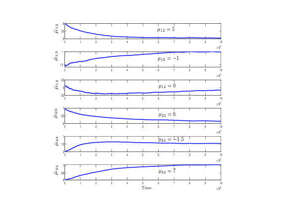
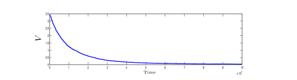
Figure 5: This figure illustrates the evolution of the estimator $\hat{\mu}$ towards; the estimator gives a very good approximation of the real dipole moment $\mu$.

Figure 6: The positive definite function $V$ defined in (20) with $\gamma_{lk}=.5$; the function decreases in average and ends up converging toward 0.

The Figures 6 and 6 illustrate the simulations of the filter equation (17) where the following constants have been used: $\gamma=0.5$, $\Gamma=1$, $A=0.01$. The simulation time $T=1e+05$ represents around 320 times the largest period of the system’s Hamiltonian $H$. This represents about 650 times the largest period of the effective Hamiltonian $H_{eff}$. Furthermore, the parameter estimator $\hat{\mu}$, the state estimator $\hat{\rho}=\hat{\Psi}\hat{\Psi}^{\dagger}$ and the real state $\rho=\Psi\Psi^{\dagger}$ are initialized at:

$$\hat{\mu}(0)=\begin{pmatrix}0&6&-1.5&.05\\ 6&0&7&-2\\ -1.5&7&0&6\\ .05&-2&6&0\\ \end{pmatrix}\quad,\quad\hat{\Psi}(0)=\begin{pmatrix}1/\sqrt{30}\\ 2/\sqrt{30}\\ 3/\sqrt{30}\\ 4/\sqrt{30}\\ \end{pmatrix}\quad,\quad\Psi(0)=\begin{pmatrix}1/2\\ 1/2\\ 1/2\\ 1/2\\ \end{pmatrix}.$$

As one can easily see, the estimator $\hat{\mu}$ ends up giving a really good approximation of the true dipole moment.

4 Robustness

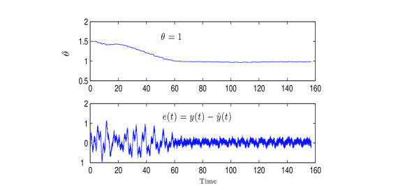
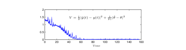
Figure 7: Here we consider the noised measurement of the form (4); the first figure illustrates the robustness, with respect to the uncertainties, in the evolution of the parameter estimator $\hat{\theta}$; the second one shows the robustness in the evolution of the error term $e(t)$.

Figure 8: The robustness in the evolution of the Lyapunov type function $V$ with $\gamma=.1$.

The laboratory noises are always present and are not negligible. These noises affect both the output result and the laser field. Moreover the delay in reading the laboratory output results are essential and must be taken into account in a faithful model. In this section, we study the robustness of the algorithm with respect to all these uncertainties through a number of simulations.

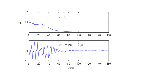
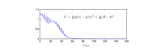
Figure 9: Here we consider the noised control field of (22); the first figure illustrates the robustness, with respect to the uncertainties, in the evolution of the parameter estimator $\hat{\theta}$; the second one shows the robustness in the evolution of the error term $e(t)$.

Figure 10: The robustness in the evolution of the Lyapunov type function $V$ with $\gamma=.1$.

Concerning the measurement output results, three kind of uncertainties can be admitted: a delay in reading the output result, a small additional constant gain and additional non-correlated noises. The simulations show that the identification algorithm, presented above, is robust with respect to all these uncertainties. The simulations of Figures 8 and 8 show this fact for the 2-level system of Section 2. Here we have considered a delay of $0.3$ (about $1/2$ of the natural period of the system) in reading the measurement results. Moreover, we have added small additional constant gains and additional non-correlated gaussian noises:

$$y(t)=\text{Tr}\left[P~{}\rho(t-0.3)\right]+0.06+0.07~{}w,$$

where $w$ has a standard normal distribution. Other simulation parameters are fixed exactly as in the Section 2.

Regarding the control input, we consider two kind of uncertainties: a small additive constant gain for the amplitude $A$ of the laser field and an additional gaussian noise for the laser field. The simulations of Figures 10 and 10, on the 2-level system of Section 2, show the robustness of the algorithm with respect to these uncertainties. Here, we have assumed that the laboratory laser field is noised as follows:

$$u(t)=(A+0.03)\sin(t)+0.07~{}w,$$ (22)

where $A=1$ as in Section 2 and $w$ is a normal distribution. Similar simulations concerning the systems of higher dimensions represent the same kind of robust behavior.

Remark 4.

One might consider additional uncertainties concerning the frequencies of the laser field (e.g. small additive constant gains in the laser frequencies). As it has been discussed in Remark 1, a more realistic estimator in the settings of our paper is given by the first averaged filter (13) ( (19) in the case of a multi-level system). The Bohr frequencies of the system do not appear in this estimator. Therefore, one can easily check that this averaged estimator represents a robust behavior with respect to the uncertainties in the laser frequencies. One only needs these frequencies to be near enough to the transition frequencies of the system ($\omega_{r}-\omega\ll A\theta$ in the case of the 2-level system).

5 Conclusion

In this paper, we propose an observer-based method for the Hamiltonian identification of a quantum system. An intuitive observer (5) has been considered for the Schrödinger equation (2.1) and has been developed and extended to give an estimate of the unknown parameters of the system. The convergence of this method is completely analyzed for a 2-level case. The multi-level cases have been addressed using heuristic arguments. Various simulations in different dimensions illustrate the relevance of the technique for these multi-dimensional systems. Finally the robustness of the design with respect to different uncertainties and noises is addressed by simulations on the 2-level case. Similar robustness results can be noted for multi-dimensional systems.

In Remark 4, it has been noted that replacing the estimator (17) with the first averaged version (19), increases considerably the robustness of the identification result with respect to the frequency uncertainties.

Such averaged filter represent even more advantages whenever the settings considered in the paper are valid. In particular, one increases considerably the robustness with respect to the delay in the measurement. Indeed, this delay only needs to be much smaller than the shortest Rabi period of the system. Secondly, the non-degeneracy assumption for the Rabi transitions $\Delta_{\Omega}$ may be removed using a slow modulation of the amplitudes $A_{lk}$. Finally, one does not really need to have access to the continuous measurement results $y_{j}(t)$ (which is lots of information to be asked in the laboratory settings). In fact, one only needs samples on the output signal with frequencies much higher than the larger Rabi frequency. All these advantages seem to highly privilege the use of the averaged estimator (19).

Appendix A Identifiability

In this appendix, we present the mathematical framework in which the identification problem can be considered. Moreover, we review briefly the former work on the identifiability of the considered system. A well-posedness result which allows us to consider the identification problem in Section 3 will be announced.

The goal is to identify $H=H_{0}+V$ or/and $\mu$ in system

$$i\frac{d}{dt}\Psi=(H_{0}+V+u(t)\mu)\Psi,\quad\Psi|_{t=0}=\Psi_{0},\quad\|\Psi_{0}\|_{{\mathcal{H}}}=1,$$ (23)

when laboratory measurements on some physical observables are provided. In [15], two different settings have been considered in order to characterize the identifiability of such a system:

(S1)

The Hamiltonian $H$ is known and the goal is to identify the dipole moment $\mu$. The so-called populations along the eigenstates $\phi_{i}$, i.e. $p_{i}=|\left<\phi_{i},\Psi(t)\right>|^{2},i=1,2,...,N$ are measured for all instants $t\geq 0$. This is performed with as many control amplitudes $u(t)$ as required.

(S2)

Neither the potential $V$ nor the dipole moment $\mu$ are known and the goal is to identify them. Note that, by identifying $H$ we mean identifying $V$, as $H_{0}$ is readily known. The eigenvalues of the Hamiltonian $H=H_{0}+V$ are also assumed to be known (this assumption is relevant in practice, see Remark 5). Here we measure the populations $p_{i}$ along the states of a canonical basis $\{e_{i}\}_{i=1}^{N}:p_{i}=|\left<e_{i},\Psi(t)\right>|^{2},i=1,2,...,N$ for all instants $t>0$ and all control amplitudes $u(t)$.

Remark 5.

It is relevant in practice to assume that the eigenvalues of the internal Hamiltonian $H=H_{0}+V$ are known. In fact the classical spectroscopy allows for identifying the eigenvalues of the Hamiltonian and discriminating between two systems that do not share the same ones. In fact spectroscopy only gives eigenvalue differences (transition frequencies), not the absolute values. The overall unknown additive factor is not seen by the measurements and has no impact on the identification result.

In this paper, we have only considered the first setting. An extension of the technique to the second setting remains to be done in future work. However,  [15] provides an identifiability result for this second setting as well.

Here we announce the identifiability result of [15] concerning the first setting. For a result in the second setting and also the proof of the result for the first setting, we refer to [15].

Theorem 2.

Suppose that there exist two dipole moments $\mu_{1}$ and $\mu_{2}$, giving rise to two evolving states $\Psi_{1}$ and $\Psi_{2}$ respectively solving

$$i\dot{\Psi}_{1} =(H+u(t)\mu_{1})\Psi_{1},$$ (24)

$$i\dot{\Psi}_{2} =(H+u(t)\mu_{2})\Psi_{2},$$ (25)

that produce identical observations for all $t\geq 0$ and all fields $u(t)$:

$$|\left<\Psi_{1}(t),\phi_{i}\right>|^{2}=|\left<\Psi_{2}(t),\phi_{i}\right>|^{2}\qquad i=1,2,...,N.$$ (26)

Then under assumptions

(A1)

Equation (24) is wavefunction controllable [25];

(A2)

The transitions of the Hamiltonian $H$ are non-degenerate: $\lambda_{i_{1}}-\lambda_{j_{1}}\neq\lambda_{i_{2}}-\lambda_{j_{2}}$ for $(i_{1},j_{1})\neq(i_{2},j_{2})$ [29];

(A3)

The diagonal part of the dipole moments $\mu_{1}$ and $\mu_{2}$, when written in the eigenbasis of the Hamiltonian $H$, is zero: $\left<\phi\right|_{i}\mu_{1}\left|\phi\right>_{i}=\left<\phi\right|_{i}\mu_{2}\left|\phi\right>_{i}=0,i=1,2,...,N$;

the two dipole moments are equal within some phase factors $\{\alpha_{i}\}_{i=1}^{N}\subset{\mathbb{R}}$ such that:

$$\forall i,j=1,2,...,N,\qquad(\mu_{1})_{ij}=e^{i(\alpha_{i}-\alpha_{j})}(\mu_{2})_{ij}.$$ (27)

Fore more details and remarks concerning the assumptions and the result of this theorem we refer to [15].

References

- [1] A. Assion, T. Baumert, M. Bergt, T. Brinxner, B. Kiefer, V. Seyfried, M. Strehle, and G. Gerber. Science, 282:919, 1998.
- [2] C. Bardeen, V. V. Yakovlev, K. R. Wilson, S. D. Carpenter, P. M. Weber, and W. S. Warren. Chem. Phys. Lett., 280:151, 1997.
- [3] C. J. Bardeen, V. V. Yakovlev, J. A. Squier, and K. R. Wilson. J. Am. Chem. Soc., 120:13023, 1998.
- [4] Y. Chen, P. Gross, V. Ramakrishna, H. Rabitz, and K. Mease. Competitive tracking of molecular objectives described by quantum mechanics. J. Chem. Phys., 102:8001–8010, 1995.
- [5] J. M. Geremia and H. Rabitz. Optimal hamiltonian identification: The synthesis of quantum optimal control and quantum inversion. J. Chem. Phys, 118(12):5369–5382, 2003.
- [6] J.M. Geremia and H. Rabitz. Optimal identification of hamiltonian information by closed-loop laser control of quantum systems. Phys. Rev. Lett., 89:263902–1–4, 2002.
- [7] J.M. Geremia, J.K. Stockton, A.C. Doherty, and H. Mabuchi. Quantum kalman filtering and the heisenberg limit in atomic magnetometry. Phys. Rev. Lett., 91:250801, 2003.
- [8] R. S. Judson and H. Rabitz. Phys. Rev. Lett., 68:1500, 1992.
- [9] H.K. Khalil. Nonlinear Systems. MacMillan, 1992.
- [10] R.L. Kosut and H. Rabitz. Identification of quantum systems. In Proceedings of the 15th IFAC World Congress, 2002.
- [11] R.L. Kosut, H. Rabitz, and I. Walmsley. Maximum likelihood identification of quantum systems for control design. In 13th IFAC Symposium on System Identification, Rotterdam, Netherlands, 2003.
- [12] R.L. Kosut, I. Walmsley, Y. Eldar, and H. Rabitz. Quantum state detector design: Optimal worst-case a posteriori performance. arXiv: quant-ph/0403150, 2004.
- [13] R.L. Kosut, I. Walmsley, and H. Rabitz. Optimal experiment design for quantum state and process tomography and Hamiltonian parameter estimation. arXiv: quant-ph/0411093, 2004.
- [14] C. Le Bris, Y. Maday, and G. Turinici. Towards efficient numerical approaches for quantum control. In Quantum Control: mathematical and numerical challenges, pages 127–142. A. Bandrauk, M.C. Delfour, and C. Le Bris, editors, CRM Proc. Lect. Notes Ser., AMS Publications, Providence, R.I., 2003.
- [15] C. Le Bris, M. Mirrahimi, H. Rabitz, and G. Turinici. Hamiltonian identifiaction for quantum systems: well-posedness and numerical approaches. ESAIM: Control, Optimization and Calculus of Variations, 2005. To appear.
- [16] R. J. Levis, G. Menkir, and H. Rabitz. Science, 292:709, 2001.
- [17] B. Li, G. Turinici, V. Ramakrishna, and H. Rabitz. Optimal dynamic discrimination of similar molecules through quantum learning control. J. Phys. Chem. B., 106(33):8125–8131, 2002.
- [18] H. Mabuchi. Dynamical identification of open quantum systems. Quantum Semiclass. Opt., 8:1103–1108, 1996.
- [19] Y. Maday and G. Turinici. New formulations of monotonically convergent quantum control algorithms. J. Chem. Phys, 118(18), 2003.
- [20] M. Mirrahimi, P. Rouchon, and G. Turinici. Lyapunov control of bilinear Schrödinger equations. Automatica, 41:1987–1994, 2005.
- [21] M. Mirrahimi, G. Turinici, and P. Rouchon. Reference trajectory tracking for locally designed coherent quantum controls. J. of Physical Chemistry A, 109:2631–2637, 2005.
- [22] M.G.A. Paris, G.M. D’Ariano, and M.F. Sacchi. Maximum likelihood method in quantum estimation. arXiv: quant-ph/0101071 v1, 2001.
- [23] Minh Q. Phan and Herschel Rabitz. Learning control of quantum-mechanical systems by laboratory identification of effective input-output maps. Chem. Phys., 217:389–400, 1997.
- [24] H. Rabitz. Perspective. shaped laser pulses as reagents. Science, 299:525–527, 2003.
- [25] V. Ramakrishna, M. Salapaka, M. Dahleh, and H. Rabitz. Controllability of molecular systems. Phys. Rev. A, 51(2):960–966, 1995.
- [26] S. Rice and M. Zhao. Optimal Control of Quantum Dynamics. Wiley, 2000. many additional references to the subjects of this paper may also be found here.
- [27] N. Shenvi, J.M. Geremia, and H. Rabitz. Nonlinear kinetic parameter identification through map inversion. J. Phys. Chem. A, 106:12315–12323, 2002.
- [28] J.K. Stockton, J.M. Geremia, A.C. Doherty, and H. Mabuchi. Robust quantum parameter estimation: Coherent magnetometry with feedback. Phys. Rev. A, 69:032109, 2004.
- [29] G. Turinici and H. Rabitz. Quantum wavefunction controllability. Chem. Phys., 267:1–9, 2001.
- [30] T. Weinacht, J. Ahn, and P. Bucksbaum. Nature, 397:233, 1999.
- [31] W. Zhu and H. Rabitz. J. Chem. Phys., 109:385, 1998.