Integrable structure of Ginibre’s ensemble of real random matrices and a Pfaffian integration theorem

Abstract

In the recent publication [E. Kanzieper and G. Akemann, Phys. Rev. Lett. 95, 230201 (2005)], an exact solution was reported for the probability $p_{n,k}$ to find exactly $k$ real eigenvalues in the spectrum of an $n\times n$ real asymmetric matrix drawn at random from Ginibre’s Orthogonal Ensemble (GinOE). In the present paper, we offer a detailed derivation of the above result by concentrating on the proof of the Pfaffian integration theorem, the key ingredient of our analysis of the statistics of real eigenvalues in the GinOE. We also initiate a study of the correlations of complex eigenvalues and derive a formula for the joint probability density function of all complex eigenvalues of a GinOE matrix restricted to have exactly $k$ real eigenvalues. In the particular case of $k=0$, all correlation functions of complex eigenvalues are determined.

,

1 Introduction

1.1 Motivation

This study grew out of our attempt to answer the question raised by A. Edelman (1997): “What is the probability $p_{n,k}$ that an $n\times n$ random real Gaussian matrix has exactly $k$ real eigenvalues?” In the physics literature, an ensemble of such random matrices is known as GinOE – Ginibre’s Orthogonal Ensemble (Ginibre 1965). Looking into this particular problem, we have realised that no comprehensive solution for the probability $p_{n,k}$ can be found without undertaking an in-depth study (Kanzieper and Akemann 2005) of the integrable structure of GinOE. The results of our investigation are reported in the present paper.

1.2 Main results

For the benefit of the readers, we collect our main results into this easy to read subsection with pointers to the sections containing detailed derivations of each statement.

1.2.1 Real part of GinOE spectrum

(I) Probability of Exactly $k$ Real Eigenvalues. Let ${\boldsymbol{\cal H}}$ be an $n\times n$ random real matrix whose entries are statistically independent random variables picked from a normal distribution $\textsf{N}(0,1)$. Then, for $n-k=2\ell$ even, the probability $p_{n,k}$ of exactly $k$ real eigenvalues occurring is

$$p_{n,k}=p_{n,n-2\ell}=\frac{p_{n,n}}{\ell!}\,Z_{(1^{\ell})}(p_{1},\cdots,p_{\ell}),$$ (1.1a)

where $$p_{n,n} p_{n,n}=2^{-n(n-1)/4} n Z_{(1^{\ell})} \ell \boldsymbol{\lambda}=(\ell_{1}^{\sigma_{1}},\cdots,\ell_{g}^{\sigma_{g}}) |\boldsymbol{\lambda}|=\ell$$ is the probability of having all eigenvalues real (Edelman 1997). The universal multivariate functions , solely determined by the number of pairs of complex conjugated eigenvalues, are so-called zonal polynomials (Macdonald 1998) that can be written as a sum over all partitions of the size

$$Z_{(1^{\ell})}(p_{1},\cdots,p_{\ell})=(-1)^{\ell}\ell!\sum_{|\boldsymbol{\lambda}|=\ell}\,\prod_{j=1}^{g}\frac{1}{\sigma_{j}!}\left(-\frac{p_{\ell_{j}}}{\ell_{j}}\right)^{\sigma_{j}}.$$ (1.1b)

A few first zonal polynomials are displayed in Table 1. The arguments $$p_{j}$$’s of the zonal polynomials are nonuniversal

$$p_{j}={\rm tr}_{(0,\lfloor n/2\rfloor-1)}\,{\boldsymbol{\hat{\varrho}}}\,^{j},$$ (1.1c)

for they depend on a nonuniversal matrix $${\boldsymbol{\hat{\varrho}}} n=2m$$. For even, its entries are

$${\hat{\varrho}}_{\alpha,\,\beta}^{\rm even} = \int_{0}^{\infty}dy\,y^{2(\beta-\alpha)-1}\,e^{y^{2}}\,{\rm erfc}(y\sqrt{2})\Big{[}(2\alpha+1)\,$$ (1.1d)

$$\times L_{2\alpha+1}^{2(\beta-\alpha)-1}(-2y^{2})+2y^{2}\,L_{2\alpha-1}^{2(\beta-\alpha)+1}(-2y^{2})\Big{]}$$

Table 1: Explicit examples of zonal polynomials $Z_{(1^{\ell})}(p_{1},\cdots,p_{\ell})$ as defined by the equation (1.1b). Another way to compute $Z_{(1^{\ell})}$ is based on the recursion equation (Macdonald 1998)

$$Z_{(1^{\ell})}(p_{1},\cdots,p_{\ell})=(\ell-1)!\,\sum_{r=0}^{\ell-1}\frac{(-1)^{\ell-r-1}}{r!}\,p_{\ell-r}\,Z_{(1^{r})}(p_{1},\cdots,p_{r})$$

supplemented by the formal “boundary” condition $Z_{(1^{0})}=1$. They are also tabulated in the manuscript by H. Jack (1976).

• $\hbox{\phantom{\footnotesize\rm 0}}\hbox{\phantom{\footnotesize\rm 0}}\boldsymbol{\lambda}$	$Z_{\boldsymbol{\lambda}}(p_{1},\cdots,p_{\ell})$
  $\hbox{\phantom{\footnotesize\rm 0}}\hbox{\phantom{\footnotesize\rm 0}}(1^{1})$	$p_{1}$
  $\hbox{\phantom{\footnotesize\rm 0}}\hbox{\phantom{\footnotesize\rm 0}}(1^{2})$	$p_{1}^{2}-p_{2}$
  $\hbox{\phantom{\footnotesize\rm 0}}\hbox{\phantom{\footnotesize\rm 0}}(1^{3})$	$p_{1}^{3}-3p_{1}p_{2}+2p_{3}$
  $\hbox{\phantom{\footnotesize\rm 0}}\hbox{\phantom{\footnotesize\rm 0}}(1^{4})$	$p_{1}^{4}+8p_{1}p_{3}-6p_{1}^{2}p_{2}+3p_{2}^{2}-6p_{4}$
  $\hbox{\phantom{\footnotesize\rm 0}}\hbox{\phantom{\footnotesize\rm 0}}(1^{5})$	$p_{1}^{5}-10p_{1}^{3}p_{2}+20p_{1}^{2}p_{3}+15p_{1}p_{2}^{2}-30p_{1}p_{4}-20p_{2}p_{3}+24p_{5}$

while for $n=2m+1$ odd,

$${\hat{\varrho}}_{\alpha,\,\beta}^{\rm odd}={\hat{\varrho}}_{\alpha,\,\beta}^{\rm even}-(-4)^{m-\beta}\frac{m!}{(2m)!}\frac{(2\beta)!}{\beta!}\,{\hat{\varrho}}_{\alpha,\,m}^{\rm even}.$$ (1.1e)

Here, the notation ${\rm erfc}(\phi)$ stands for the complementary error function,

$${\rm erfc}(\phi)=\frac{2}{\sqrt{\pi}}\,\int_{\phi}^{\infty}dt\,e^{-t^{2}},$$

while $L_{j}^{\alpha}(\phi)$ denote the generalised Laguerre polynomials

$$L_{j}^{\alpha}(\phi)=\frac{1}{j!}\phi^{-\alpha}\,e^{\phi}\,\frac{d^{\,j}}{d\phi^{\,j}}\left(\phi^{\,j+\alpha}\,e^{-\phi}\right).$$

The above result (1.1a) will be derived in Section 6.

(II) Generating Function For Probabilities $p_{n,k}$. The generating function $G_{n}(z)$ for the probabilities $p_{n,k}$ is

$$G_{n}(z)=\sum_{\ell=0}^{\lfloor n/2\rfloor}z^{\ell}p_{n,n-2\ell}=p_{n,n}\,{\rm det}\,\big{[}{\boldsymbol{\hat{1}}}+z\,{\boldsymbol{\hat{\varrho}}}\big{]}_{\lfloor n/2\rfloor\times\lfloor n/2\rfloor}.$$ (1.1b)

Equation (1.1b) with the ${\boldsymbol{\hat{\varrho}}}$ of needed parity provides us with yet another way of computing the entire set of $p_{n,k}$’s at once! Table 2 contains a comparison of our analytic predictions with numeric simulations. The result (1.1b) will be proven in Section 6.

(III) Probability $p_{n,n-2}$ of Exactly One Pair of Complex Conjugated Eigenvalues. For $k=n-2$, the probability function $p_{n,k}$ reduces to

$$p_{n,n-2}=2\,p_{n,n}\,\int_{0}^{\infty}dy\,y\,e^{y^{2}}\,{\rm erfc}(y\sqrt{2})\,L_{n-2}^{2}(-2y^{2}).$$ (1.1ca)

An alternative expression reads:

$$p_{n,n-2}=p_{n,n}\,\left[\sqrt{2}\,\sum_{j=0}^{\lfloor n/2\rfloor-1}3^{j+\alpha_{n}/2}\,P_{2j+\alpha_{n}}\left(\frac{2}{\sqrt{3}}\right)-\lfloor n/2\rfloor\right].$$ (1.1cb)

Here, $$\alpha_{n}=\lceil n/2\rceil-\lfloor n/2\rfloor P_{n}(\phi)$$, and stands for the Legendre polynomials

$$P_{j}(\phi)=\frac{(-1)^{j}}{2^{j}j!}\,\frac{d^{j}}{d\phi^{j}}\left[(1-\phi^{2})^{j}\right].$$

The leading large-$$n p_{n,n-2}$$ behaviour of the probability is given by

$$p_{n,n-2}\approx\frac{3^{n+1/2}}{8\sqrt{\pi\,n}}\,p_{n,n}.$$ (1.1cc)

The above three results will be derived in Section 4.1, Section 7.1 and Section 7.2, respectively.

1.2.2 Complex part of GinOE spectrum

(IV) Joint Probability Density Function of All Complex Eigenvalues Given There Are $k$ Real Eigenvalues. Let ${\boldsymbol{\cal H}_{k}}$ be an $n\times n$ random real matrix with $k$ real eigenvalues such that its entries are statistically independent random variables picked from a normal distribution $\textsf{N}(0,1)$. Then, the joint probability density function (j.p.d.f.) of its $2\ell=n-k$ complex eigenvalues is

Table 2: Exact solution for $p_{12,k}$ (first and second column) compared to numeric simulations (third column) performed by direct diagonalisation of $1,000,000$ of $12\times 12$ matrices.

	Analytic solution
			Numeric
$k$	Exact	Approximate	simulation
$\00$	$\,\frac{29930323227453-20772686238032\sqrt{2}}{17592186044416}\,$	0.031452	0.031683
$\02$	$\,\frac{3(1899624551312\sqrt{2}-2060941421503)}{4398046511104}$	0.426689	0.427670
$\04$	$\,\frac{3(2079282320189-505722262348\sqrt{2})}{8796093022208}$	0.465235	0.464098
$\06$	$\,\frac{252911550974\sqrt{2}-27511352125}{4398046511104}$	0.075070	0.075021
$\08$	$\,\frac{15(1834091507-10083960\sqrt{2})}{17592186044416}$	0.001552	0.001526
$10$	$\,\frac{3(1260495\sqrt{2}-512)}{2199023255552}$	0.000002	0.000002
$12$	$\,\frac{1}{8589934592}$	0.000000	0.000000

$$P_{{\boldsymbol{\cal H}_{k}}}(z_{1},\cdots,z_{\ell}) =\frac{p_{n,n}}{\ell!}\,\left(\frac{2}{i}\right)^{\ell}\,$$ (1.1cf)

$$\times\prod_{j=1}^{\ell}\,{\rm erfc}\left(\frac{z_{j}-{\bar{z}}_{j}}{i\sqrt{2}}\right)\,{\rm pf\,}\left[\begin{array}[]{cc}{\cal D}_{n}(z_{i},z_{j})&{\cal D}_{n}(z_{i},{\bar{z}}_{j})\\ {\cal D}_{n}({\bar{z}}_{i},z_{j})&{\cal D}_{n}({\bar{z}}_{i},{\bar{z}}_{j})\\ \end{array}\right]_{2\ell\times 2\ell}.$$

Here, ${\rm pf}$ denotes the Pfaffian. The above j.p.d.f. is supported for $({\rm Re\,}z_{1},\cdots,{\rm Re\,}z_{\ell})\in{\mathbb{R}}^{\ell}$, and $({\rm Im\,}z_{1},\cdots,{\rm Im\,}z_{\ell})\in({\mathbb{R}}^{+})^{\ell}$. The antisymmetric kernel ${\cal D}_{n}(z,z^{\prime})$ is given explicitly by (1.1cghp) – (1.1cghv) of Section 3 where the statement (1.1cf) is proven.

(V) Correlation Functions of Complex Eigenvalues in The Spectra Free of Real Eigenvalues. Let ${\boldsymbol{\cal H}_{0}}$ be an $n\times n$ random real matrix with no real eigenvalues such that its entries are statistically independent random variables picked from a normal distribution $\textsf{N}(0,1)$. Then, the $p$-point correlation function ($1\leq p\leq\ell$) of its complex eigenvalues, defined by (2.3), equals

$$R^{({\boldsymbol{\cal H}}_{0})}_{0,p}(z_{1},\cdots,z_{p};n)=p_{n,n}\,\frac{\prod_{j=0}^{\ell-1}r_{j}}{\prod_{j=1}^{n}\Gamma(j/2)}\prod_{j=1}^{p}{\rm erfc}\left(\frac{z_{j}-{\bar{z}}_{j}}{i\sqrt{2}}\right)\,\exp\left(-\frac{z_{j}^{2}+{\bar{z}}_{j}^{2}}{2}\right)$$

$$\times\,{\rm pf\,}\left[\begin{array}[]{cc}\kappa_{\ell}(z_{i},z_{j})&\kappa_{\ell}(z_{i},{\bar{z}}_{j})\\ \kappa_{\ell}({\bar{z}}_{i},z_{j})&\kappa_{\ell}({\bar{z}}_{i},{\bar{z}}_{j})\\ \end{array}\right]_{2p\times 2p}.$$ (1.1cgc)

Here, $$n=2\ell \kappa_{\ell}$$ and the ‘pre-kernel’ equals

$$\kappa_{\ell}(z,z^{\prime})=i\sum_{j=0}^{\ell-1}\frac{1}{r_{j}}\bigg{[}p_{2j}(z)p_{2j+1}(z^{\prime})-p_{2j}(z^{\prime})p_{2j+1}(z)\bigg{]}.$$ (1.1cgd)

The polynomials $$p_{j}(z) {\rm Im\,}z>0$$ are skew orthogonal in the complex half-plane ,

$$\langle p_{2j+1},p_{2k}\rangle_{\rm c}=-\langle p_{2k},p_{2j+1}\rangle_{\rm c}=i\,r_{j}\,\delta_{jk},$$ (1.1cge)

$$\langle p_{2j+1},p_{2k+1}\rangle_{\rm c}=\langle p_{2j},p_{2k}\rangle_{\rm c}=0,$$ (1.1cgf)

with respect to the skew product

$$\langle f,g\rangle_{\rm c}=\int_{{\rm Im\,}z>0}d^{2}z\,{\rm erfc}\left(\frac{z-{\bar{z}}}{i\sqrt{2}}\right)\,\exp\left(-\frac{z^{2}+{\bar{z}}^{2}}{2}\right)\,\left[f(z)g({\bar{z}})-f({\bar{z}})g(z)\right].$$ (1.1cgg)

For detailed derivation, a reader is referred to Section 8 which also addresses the problem of calculating the probability $p_{n,0}$ to find no real eigenvalues in the spectrum of GinOE.

1.2.3 How to integrate a Pfaffian?

All the results announced so far would have not been derived without a Pfaffian integration theorem that we consider to be a major technical achievement of our study. Conceptually, it is based on a new, topological, interpretation of the ordered Pfaffian expansion as introduced in Section 5.

(VI) The Pfaffian Integration Theorem. Let $d\pi(z)$ be any benign measure on $z\in{\mathbb{C}}$, and the function $Q_{n}(x,y)$ be an antisymmetric function of the form

$$Q_{n}(x,y)=\frac{1}{2}\sum_{j,k=0}^{n-1}q_{j}(x)\,{\hat{\mu}}_{jk}\,q_{k}(y)$$ (1.1cgha)

where $$q_{j} j {\boldsymbol{\hat{\mu}}}$$’s are arbitrary polynomials of -th order, and is an antisymmetric matrix. Then the integration formula

$$\left(\frac{2}{i}\right)^{\ell}\prod_{j=1}^{\ell}\,\int_{z_{j}\in{\mathbb{C}}}d\pi(z_{j})\,\, {\rm pf\,}\left[\begin{array}[]{cc}Q_{n}(z_{i},z_{j})&Q_{n}(z_{i},{\bar{z}}_{j})\\ Q_{n}({\bar{z}}_{i},z_{j})&Q_{n}({\bar{z}}_{i},{\bar{z}}_{j})\\ \end{array}\right]_{2\ell\times 2\ell}$$ (1.1cghd)

$$=Z_{(1^{\ell})}\left(\frac{1}{2}{\rm tr}_{(0,n-1)}{\boldsymbol{\hat{\upsilon}}}^{1},\cdots,\frac{1}{2}{\rm tr}_{(0,n-1)}{\boldsymbol{\hat{\upsilon}}}^{\ell}\right)$$ (1.1cghe)

holds, provided the integrals in its l.h.s. exist. Here, $$Z_{(1^{\ell})} \ell {\boldsymbol{\hat{\upsilon}}}$$ are zonal polynomials whose arguments are determined by a matrix with the entries

$${\hat{\upsilon}}_{\alpha,\beta}=i\sum_{k=0}^{n-1}{\hat{\mu}}_{\alpha,k}\int_{z\in{\mathbb{C}}}d\pi(z)\left[q_{k}(z)\,q_{\beta}({\bar{z}})-q_{\beta}(z)\,q_{k}({\bar{z}})\right].$$ (1.1cghf)

This theorem that can be viewed as a generalisation of the Dyson integration theorem (Dyson 1970, Mahoux and Mehta 1991) will be proven in Section 5.

Interestingly, the Pfaffian integration theorem is not listed in the classic reference book (Mehta 2004) on the Random Matrix Theory (RMT). Also, we are not aware of any other RMT literature reporting this result which may have implications far beyond the scope of the present paper.

1.3 A guide through the paper

Having announced the main results of our study, we defer plunging into formal mathematical proofs of the above six statements until Section 3. Instead, in Section 2, we deliberately draw the reader’s attention to a comparative analysis of GinOE and two other representatives of non-Hermitean random matrix models known as Ginibre’s Unitary (GinUE) and Ginibre’s Symplectic (GinSE) Ensemble. Starting with the definitions of the three ensembles, we briefly discuss their diverse physical applications, pinpoint qualitative differences between their spectra, and present a detailed comparative analysis of major structural results obtained for GinUE, GinSE and GinOE since 1965. We took great pains to write a review-style Section 2 in order (i) to help the reader better appreciate a profound difference between GinOE and the two other non-Hermitean random matrix ensembles on both qualitative and structural levels as well as (ii) place our own work in a more general context.

A formal analysis starts with Section 3 devoted to a general consideration of statistics of real eigenvalues. Its first part, Section 3.1, summarises previously known analytic results (Edelman 1997) for the probability function $p_{n,k}$ of the fluctuating number of real eigenvalues in the spectrum of GinOE. Section 3.2 deals with the joint probability density function of complex eigenvalues of GinOE random matrices that have a given number of real eigenvalues. The Pfaffian representation (1.1cf) is the main outcome of Section 3.2. This result is further utilised in Section 3.3 where the probability function $p_{n,k}$ is put into the form of a ‘Pfaffian integral’ (3.3). The analysis of the latter expression culminates in concluding that the Dyson integration theorem, a standard tool of Random Matrix Theory, is inapplicable for treating the Pfaffian integral obtained. The latter task will be accomplished in Section 5.

Section 4 attacks the probability function $p_{n,k}$ for a few particular values of $k$. The probabilities $p_{n,n-2}$, $p_{n,n-4}$ and $p_{n,n-6}$ of one, two, and three pairs of complex conjugated eigenvalues occurring are treated in Section 4.1, Section 4.2 and 4.3, respectively. This is done by explicit calculation of the Pfaffian in (3.3) followed by a term-by-term integration of the resulting Pfaffian expansion. In Section 4.4, we briefly discuss a faster-than-exponential growth of the number of terms in this expansion caused by further decrease of $k$.

Section 5, devoted to the Pfaffian integration theorem, is central to the paper. Its main objective is to introduce a topological interpretation of the terms arising in a permutational expansion of the Pfaffian in the l.h.s. of (1.1cghd). Such a topological interpretation turns out to be the proper language in the subsequent proof of the Pfaffian integration theorem. In Section 5.1, the Pfaffian integration theorem is formulated and discussed in the light of the Dyson integration theorem. In Section 5.2, an ordered permutational Pfaffian expansion is defined and interpreted in topological terms. The notions of strings, substrings, loop-like strings and loop-like substrings for certain subsets of terms arising in an ordered Pfaffian expansion are introduced and illustrated on simple examples in Sections 5.2.1 and 5.2.2. Further, equivalent strings and equivalent classes of strings are defined and counted. The issue of decomposition of strings into a set of loop-like substrings is also considered in detail (Lemma 5.2). Section 5.2.3 is devoted to the counting of loop-like strings. In Section 5.2.4, the notion of adjacent strings is introduced and illustrated. Adjacent strings are counted in Lemma 5.4. Their relation to loop-like strings is discussed in Lemma 5.5. Section 5.2.5 deals with a characterisation of adjacent strings by their handedness; adjacent strings of a given handedness are counted there, too. In Section 5.2.6, equivalent classes of adjacent strings are defined, counted, and explicitly built. Section 5.3 and Section 5.4 are preparatory for Section 5.5, where the Pfaffian integration theorem is eventually proven. For the readers’ benefit, a vocabulary of the topological terms we use is summarised in Table 3.

Section 6 utilises the Pfaffian integration theorem to obtain a general solution for the sought probability function $p_{n,k}$ (Section 6.1), derive a determinantal expression for the entire generating function of $p_{n,k}$’s (Section 6.2), and address the issue of integer moments of the fluctuating number of real eigenvalues in GinOE spectra (Section 6.3).

Section 7 is devoted to the probability $p_{n,n-2}$ for two complex conjugated pairs of eigenvalues to occur; a large-$n$ analysis of $p_{n,n-2}$ is also presented there.

Section 8 discusses the Pfaffian structure of the $p$-point correlation functions of complex eigenvalues belonging to spectra of a subclass of GinOE matrices without real eigenvalues. The same section addresses the problem of calculating the probability $p_{n,0}$ to find no real eigenvalues in spectra of GinOE.

Section 9 contains conclusions with the emphasis placed on open problems. The most involved technical calculations are collected in four appendices.

2 Comparative analysis of GinOE, GinUE, and GinSE

2.1 Definition and consequences of violated Hermiticity

Ginibre’s three random matrix models – GinOE, GinUE, and GinSE – were derived from the celebrated Gaussian Orthogonal (GOE), Gaussian Unitary (GUE), and Gaussian Symplectic (GSE) random matrix ensembles in a purely formal way by dropping the Hermiticity constraint. Consequently, the non-Hermitean descendants of GOE, GUE and GSE share the same Gaussian probability density function

$$P_{\beta}[{\boldsymbol{\cal H}}]=(\pi a_{\beta})^{-\beta n^{2}/2}\exp\left[-a_{\beta}^{-1}\,{\rm tr\,}\left({\boldsymbol{\cal H}}{\boldsymbol{\cal H}}^{\dagger}\right)\right],\;\;\;{\boldsymbol{\cal H}}^{\dagger}\neq{\boldsymbol{\cal H}},\;\;\;\beta=1,2,4,$$ (1.1cgha)

for a matrix “Hamiltonian” ${\boldsymbol{\cal H}}\in{\mathbb{T}}_{\beta}(n)$ to occur; the constant $a_{\beta}$ is chosen to be $a_{\beta}=2-\delta_{\beta,2}$ (this slightly differs from the convention used in the original paper by Ginibre). However, the spaces ${\mathbb{T}}_{\beta}$ on which the matrices ${\boldsymbol{\cal H}}$ vary are different: ${\mathbb{T}}_{1}(n)$, ${\mathbb{T}}_{2}(n)$, and ${\mathbb{T}}_{4}(n)$ span all $n\times n$ matrices with real (GinOE, $\beta=1$), complex (GinUE, $\beta=2$), and real quaternion (GinSE, $\beta=4$) entries, respectively.

The violated Hermiticity, ${\boldsymbol{\cal H}}^{\dagger}\neq{\boldsymbol{\cal H}}$, brings about the two major phenomena: (i) complex-valuedness of the random matrix spectrum and (ii) splitting the random matrix eigenvectors into a bi-orthogonal set of left and right eigenvectors. Statistics of complex eigenvalues, including their joint probability density function, and statistics of left and right eigenvectors of a random matrix ${\boldsymbol{\cal H}}\in{\mathbb{T}}_{\beta}$ drawn from (1.1cgha) are of primary interest.

Only the spectral statistics will be addressed in the present paper. (For studies of the eigenvector statistics in GinUE, the reader is referred to the papers by Chalker and Mehlig (1998), Mehlig and Chalker (2000), and Janik et al (1999). We are not aware of any results for eigenvector statistics in GinSE and GinOE.)

2.2 Physical applications

While the ensemble definition (1.1cgha) was born out of pure mathematical curiosity , non-Hermitean random matrices have surfaced in various fields of knowledge by E. Wigner’s “miracle of the appropriateness” (Wigner 1960). From the physical point of view, non-Hermitean random matrices have proven to be as important as their Hermitean counterparts. (For a detailed exposition of physical applications of Hermitean RMT we refer to the review by Guhr et al (1998)).

Random matrices drawn from GinUE appear in the description of dissipative quantum maps (Grobe et al 1988, Grobe and Haake 1989) and in the characterisation of two-dimensional random space-filling cellular structures (Le Cäer and Ho 1990, Le Cäer and Delannay 1993).

Ginibre’s Orthogonal Ensemble of random matrices arises in the studies of dynamics (Sommers et al 1988, Sompolinsky et al 1988) and of synchronisation effect (Timme et al 2002, Timme et al 2004) in random networks; GinOE is also helpful in the statistical analysis of cross-hemisphere correlation matrix of the cortical electric activity (Kwapień et al 2000) as well as in the understanding of inter-market financial correlations (Kwapień et al 2006).

All three Ginibre ensembles (GinOE, GinUE, GinSE) arise in the context of directed “quantum chaos” (Efetov 1997a, Efetov 1997b, Kolesnikov and Efetov 1999, Fyodorov et al 1997, Markum et al 1999). Their chiral counterparts (Stephanov 1996, Halasz et al 1997, Osborn 2004, Akemann 2005) help elucidate universal aspects of the phenomenon of spontaneous chiral symmetry breaking in quantum chromodynamics (QCD) with chemical potential: the presence or absence of real eigenvalues in the complex spectrum singles out different chiral symmetry breaking patterns. For a review of QCD applications of non-Hermitean random matrices with built-in chirality, the reader is referred to Akemann (2007).

Other recent findings (Zabrodin 2003) associate statistical models of non-Hermitean normal random matrices with integrable structures of conformal maps and interface dynamics at both classical (Mineev-Weinstein et al 2000) and quantum (Agam et al 2002) scales. For a comprehensive review of these and other physical applications, the reader is referred to the survey paper by Fyodorov and Sommers (2003).

2.3 Spectral statistical properties of Ginibre’s random matrices

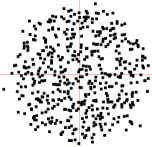
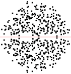
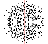
Figure 1: Numerically simulated distributions of complex eigenvalues in GinUE (left panel), GinSE (middle panel), and GinOE (right panel). Three different eigenvalue patterns are clearly observed. Eigenvalues are scattered almost uniformly in GinUE, depleted from the real axis in GinSE, and accumulated along the real axis in GinOE.

A profound difference between spectral patterns of the three non-Hermitean random matrix models has been realised long ago. Anticipated in the early papers by Ginibre (1965) and Mehta and Srivastava (1966), it was further confirmed analytically by using varied techniques (Edelman 1997, Efetov 1997a, Efetov 1997b, Kolesnikov and Efetov 1999, Kanzieper 2002a, Kanzieper 2002b, Nishigaki and Kamenev 2002, Splittorff and Verbaarschot 2004, Kanzieper 2005, Akemann and Basile 2007).

Qualitatively, there is a general consensus that (i) the spectrum of GinUE is approximately characterised by a uniform density of complex eigenvalues. This is not the case for the two other ensembles. (ii) In GinSE, the density of complex eigenvalues is smooth but the probability density of real eigenvalues tends to zero. This corresponds to a depletion of the eigenvalues along the real axis. (iii) On the contrary, the density of eigenvalues in GinOE exhibits an accumulation of the eigenvalues along the real axis. It is the latter phenomenon that will be quantified in our paper.

Our immediate goal here is to highlight the inter-relation between these qualitative features of the complex spectra and the formal structures underlying Ginibre’s random matrix ensembles. To this end, we present a brief comparative review of the major structural results obtained for all three Ginibre’s ensembles (GinUE, GinSE, and GinOE) since 1965, in the order of increasing difficulty of their treatment.

Joint Probability Density Function of All $n$ Eigenvalues. In this subsection, we collect explicit results for the joint probability density functions of all $n$ complex eigenvalues of a random matrix ${\boldsymbol{\cal H}}\in{\mathbb{T}}_{\beta}(n)$ drawn from any of the three Ginibre random matrix ensembles.

• GinUE: The spectrum of a random matrix ${\boldsymbol{\cal H}}\in{\mathbb{T}}_{2}(n)$ drawn from GinUE consists of $n$ complex eigenvalues $(z_{1},\cdots z_{n})$ whose joint probability density function mirrors (Ginibre 1965) that of GUE (see, e.g., Mehta 2004),

  $$P_{n}^{(2)}(z_{1},\cdots,z_{n})=\left(\pi^{n}\prod_{\ell=1}^{n}\ell!\right)^{-1}\prod_{\ell_{1}>\ell_{2}=1}^{n}|z_{\ell_{1}}-z_{\ell_{2}}|^{2}\prod_{\ell=1}^{n}e^{-z_{\ell}{\bar{z}}_{\ell}}.$$ (1.1cghb)

  Similarly to the electrostatic model introduced by E. Wigner (1957), J. Ginibre pointed out that the j.p.d.f. (1.1cghb) can be thought of as that describing the distribution of the positions of charges of a two-dimensional Coulomb gas in an harmonic oscillator potential $U(z)=|z|^{2}/2$, at the inverse temperature $1/T=2$.
  

• GinSE: The spectrum of a random matrix ${\boldsymbol{\cal H}}\in{\mathbb{T}}_{4}(n)$ drawn from GinSE consists of $n$ pairs of complex conjugated eigenvalues $(z_{1},{\bar{z}}_{1},\cdots,z_{n},{\bar{z}}_{n})$. The corresponding joint probability density function was derived by Ginibre (1965),

  $$P_{n}^{(4)}(z_{1},\cdots,z_{n}) =\left((2\pi)^{n}n!\prod_{\ell=1}^{n}(2\ell-1)!\right)^{-1}\,\prod_{\ell_{1}>\ell_{2}=1}^{n}|z_{\ell_{1}}-z_{\ell_{2}}|^{2}|z_{\ell_{1}}-{\bar{z}}_{\ell_{2}}|^{2}$$ (1.1cghc)

  $$\times\prod_{\ell=1}^{n}|z_{\ell}-{\bar{z}}_{\ell}|^{2}\,\exp(-z_{\ell}{\bar{z}}_{\ell}).$$

  Notice that the factor $\prod_{\ell=1}^{n}|z_{\ell}-{\bar{z}}_{\ell}|^{2}\,$ in (1.1cghc) is directly responsible for the depletion of the eigenvalues along the real axis. For GinSE, a physical analogy with a two-dimensional Coulomb gas is much less transparent; it has been discussed by P. Forrester (2005).
  

• GinOE: Contrary to GinUE and GinSE, the complex spectrum $(w_{1},\cdots,w_{n})$ of a random matrix ${\boldsymbol{\cal H}}\in{\mathbb{T}}_{1}(n)$ drawn from GinOE generically contains a finite fraction of real eigenvalues; the remaining complex eigenvalues always form complex conjugated pairs. Indeed, no other option is allowed by the real secular equation ${\rm det\,}(w-{\boldsymbol{\cal H}})=0$ determining the eigenvalues of ${\boldsymbol{\cal H}}$.
  
  This very peculiar feature of GinOE, that we call accumulation of the eigenvalues along the real axis, can conveniently be accommodated by dividing the entire space ${\mathbb{T}}_{1}(n)$ spanned by all real $n\times n$ matrices ${\boldsymbol{\cal H}}\in{\mathbb{T}}_{1}(n)$ into $(n+1)$ mutually exclusive sectors ${\mathbb{T}}_{1}(n/k)$ associated with the matrices ${\boldsymbol{\cal H}_{k}}\subset{\boldsymbol{\cal H}}$ having exactly $k$ real eigenvalues, such that ${\mathbb{T}}_{1}(n)=\bigcup_{k=0}^{n}{\mathbb{T}}_{1}(n/k)$. The sectors ${\mathbb{T}}_{1}(n/k)$, characterised by the partial j.p.d.f.’s $P_{{\boldsymbol{\cal H}}\in{\mathbb{T}}_{1}(n/k)}(w_{1},\cdots,w_{n})$, can be explored separately because they contribute additively to the j.p.d.f. of all $n$ eigenvalues of ${\boldsymbol{\cal H}}$ from ${\mathbb{T}}_{1}(n)$:

  $$P_{n}^{(1)}(w_{1},\cdots,w_{n})=\sum_{k=0}^{n}P_{{\boldsymbol{\cal H}}\in{\mathbb{T}}(n/k)}(w_{1},\cdots,w_{n}).$$ (1.1cghd)

  In entire generality, the partial j.p.d.f.’s have been determined by Lehmann and Sommers (1991) who proved, a quarter of a century after Ginibre’s work, that the $k$-th partial j.p.d.f. ($0\leq k\leq n$) equals

  $$P_{{\boldsymbol{\cal H}}\in{\mathbb{T}}(n/k)}(\lambda_{1},\cdots,\lambda_{k};z_{1},\cdots,z_{\ell})$$

  $$=\frac{2^{\ell-n(n+1)/4}}{i^{\ell}\,k!\,\ell!\,\prod_{j=1}^{n}\Gamma(j/2)}\prod_{i>j=1}^{k}|\lambda_{i}-\lambda_{j}|\,\prod_{j=1}^{k}\,\exp(-\lambda_{j}^{2}/2)$$

  $$\times\prod_{j=1}^{k}\prod_{i=1}^{\ell}(\lambda_{j}-z_{i})(\lambda_{j}-{\bar{z}}_{i})\,\prod_{i>j=1}^{\ell}|z_{i}-z_{j}|^{2}|z_{i}-{\bar{z}}_{j}|^{2}\,$$

  $$\times\prod_{j=1}^{\ell}\,(z_{j}-{\bar{z}}_{j})\,{\rm erfc}\left(\frac{z_{j}-{\bar{z}}_{j}}{i\sqrt{2}}\right)\,\exp\left(-\frac{z_{j}^{2}+{\bar{z}}_{j}^{2}}{2}\right).$$ (1.1cghe)

  Here, the parameterisation $(w_{1},\cdots,w_{n})=(\lambda_{1},\cdots,\lambda_{k};z_{1},{\bar{z}}_{1},\cdots,z_{\ell},{\bar{z}}_{\ell})$ was used to indicate that the spectrum is composed of $k$ real and $2\ell$ complex eigenvalues so that $k+2\ell=n$. The above j.p.d.f. is supported for $(\lambda_{1},\cdots,\lambda_{k})\in{\mathbb{R}}^{k}$, $({\rm Re}\,z_{1},\cdots,{\rm Re}\,z_{\ell})\in{\mathbb{R}}^{\ell}$, and $({\rm Im}\,z_{1},\cdots,{\rm Im}\,z_{\ell})\in({\mathbb{R}}^{+})^{\ell}$. Notice that since the complex eigenvalues come in $\ell$ conjugated pairs, the identity $n=2\ell+k$ implies that half of the sets ${\mathbb{T}}_{1}(n/k)$ are empty: this happens whenever $n$ and $k$ are of different parity.
  
  In writing (• ‣ 2.3), we have used a representation due to Edelman (1997) who rediscovered the result by Lehmann and Sommers (1991) a few years later. The particular case $k=n$ of (• ‣ 2.3), corresponding to the matrices ${\boldsymbol{\cal H}}\in{\mathbb{T}}(n/n)$ with all eigenvalues real, was first derived by Ginibre (1965). No physical interpretation of the distribution (• ‣ 2.3) in terms of a two-dimensional Coulomb gas is known as yet.

Eigenvalue Correlation Functions and Inapplicability of the Dyson Integration Theorem to the Description of GinOE. Spectral statistical properties of random matrices can be retrieved from a set of spectral correlation functions defined as

$$R_{p}^{(\beta)}(z_{1},\cdots,z_{p};n)=\frac{n!}{(n-p)!}\,\prod_{j=p+1}^{n}\int_{\mathbb{C}}d^{2}z_{j}\,P_{n}^{(\beta)}(z_{1},\cdots,z_{n}),\;\;\;\beta=2,\;4$$ (1.1cghf)

for GinUE ($\beta=2$) and GinSE ($\beta=4$), and

$$R_{p,q}^{({\boldsymbol{\cal H}}_{k})}(\lambda_{1},\cdots,\lambda_{p};z_{1},\cdots,z_{q};n)=\frac{k!}{(k-p)!}\frac{\ell!}{(\ell-q)!}$$

$$\times\,\prod_{j=p+1}^{k}\int_{\mathbb{R}}d\lambda_{j}\prod_{m=q+1}^{\ell}\int_{\mathbb{C}}d^{2}z_{m}\,\,P_{{\boldsymbol{\cal H}}\in{\mathbb{T}}(n/k)}(\lambda_{1},\cdots,\lambda_{k};z_{1},\cdots,z_{\ell}),$$ (1.1cghg)

for GinOE ($\beta=1$). The GinOE correlation function refers to the spectrum of matrices ${\boldsymbol{\cal H}_{k}}\subset{\boldsymbol{\cal H}}$ having exactly $k$ real eigenvalues.

The analytic calculation of the above correlation functions is one of the major operational tasks of the non-Hermitean RMT. Whenever feasible, such a calculation either explicitly rests on or can eventually be traced back to the three concepts: (i) a determinant (or Pfaffian) representation of the j.p.d.f.’s of all eigenvalues, (ii) a projection property of the kernel function associated with the aforementioned determinant representation, and (iii) the Dyson integration theorem (Dyson 1970, Mahoux and Mehta 1991) that makes use of both (i) and (ii). Highly successful in the Hermitean RMT, the above three concepts are not always at work in the non-Hermitean RMT. Particularly, the Dyson integration theorem, being effective for GinUE and GinSE (see below), fails to work for GinOE.

It will be argued that a mixed character of the GinOE spectrum consisting of both complex and purely real eigenvalues is the direct cause of the failure. For the readers convenience as well as for the future reference, we cite the Dyson integration theorem below (Mehta (1976); see also Theorem 5.1.4 in Mehta’s book (2004)).
Theorem 2.1 (Dyson integration theorem). Let $f(x,y)$ be a function with real, complex or quaternion values, such that

$${\bar{f}}(x,y)=f(y,x),$$ (1.1cghha)

where $${\bar{f}}=f f {\bar{f}} {\bar{f}} f$$ if is real, is the complex conjugate if it is complex, and is the dual of if it is quaternion. Assume that

$$\int\,d\pi(y)\,f(x,y)\,f(y,z)\,=f(x,z)+\lambda\,f(x,z)-f(x,z)\,\lambda,$$ (1.1cghhb)

where $$\lambda d\pi [f(x_{i},x_{j})]_{n\times n} n\times n (i,j) f(x_{i},x_{j})$$ is a constant quaternion and is a suitable measure. Let denote the matrix with its element equal to . Then,

$$\int\,d\pi(x_{n})\,{\rm det}[f(x_{i},x_{j})]_{n\times n}\,=(c-n+1)\,{\rm det}[f(x_{i},x_{j})]_{(n-1)\times(n-1)}$$ (1.1cghhc)

with

$$c=\int\,d\pi(x)\,f(x,x).$$ (1.1cghhd)

When $f(x,y)$ is real or complex, the quaternion constant $\lambda$ vanishes. For $f(x,y)$ taking quaternion values, $\det$ should be replaced by ${\rm qdet}$, the quaternion determinant (Dyson 1972).
This theorem prompts the following definition.
Definition 2.1. A function $f(x,y)$ satisfying the first and the second equation in the Dyson integration theorem is said to obey the projection property.

Being equipped with the above reminder, we are ready to present, and discuss, a collection of formulae available for the $p$-point correlation functions in Ginibre’s ensembles.

• GinUE: The joint probability density function (1.1cghb) of all $n$ eigenvalues is reducible to a determinant form (Ginibre 1965)

  $$P_{n}^{(2)}(z_{1},\cdots,z_{n})=\frac{1}{n!}\,{\rm det}\left[K_{n}^{(2)}(z_{k},z_{\ell})\right]_{n\times n}\prod_{j=1}^{n}e^{-z_{j}{\bar{z}}_{j}}$$ (1.1cghi)

  with $K_{n}^{(2)}(z,z^{\prime})$ being a two-point scalar kernel

  $$K_{n}^{(2)}(z,z^{\prime})=\frac{1}{\pi}\sum_{\ell=0}^{n-1}\frac{(z{\bar{z}}^{\prime})^{\ell}}{\Gamma(\ell+1)}.$$ (1.1cghj)

  Since it obeys the projection property, the Dyson Integration Theorem brings a determinant expression for the $p$-point correlation function:

  $$R_{p}^{(2)}(z_{1},\cdots,z_{p};n)={\rm det}\left[K_{n}^{(2)}(z_{k},z_{\ell})\right]_{p\times p}\prod_{j=1}^{p}e^{-z_{j}{\bar{z}}_{j}}.$$ (1.1cghk)

  These results, first derived by J. Ginibre (1965), provide a comprehensive description of spectral fluctuations in GinUE.
  

• GinSE: The joint probability density function (1.1cghc) of all $n$ eigenvalues is reducible to a quaternion determinant form (Mehta and Srivastava 1966)

  $$P_{n}^{(4)}(z_{1},\cdots,z_{n})=\frac{1}{n!}\,{\rm qdet}\left[K_{n}^{(4)}(z_{k},z_{\ell})\right]_{n\times n}\prod_{j=1}^{n}({\bar{z}}_{j}-z_{j})\,e^{-z_{j}{\bar{z}}_{j}},$$ (1.1cghl)

  where $K_{n}^{(4)}(z,z^{\prime})$ is a quaternion whose $2\times 2$ matrix representation reads (Kanzieper 2002a)

  $$\Theta[K_{n}^{(4)}(z,z^{\prime})]=\left(\begin{array}[]{cc}-\kappa_{n}^{(4)}({\bar{z}},z^{\prime})&-\kappa_{n}^{(4)}({\bar{z}},{\bar{z}}^{\prime})\\ \kappa_{n}^{(4)}(z,z^{\prime})&\kappa_{n}^{(4)}(z,{\bar{z}}^{\prime})\end{array}\right).$$ (1.1cgho)

  Here,

  $$\kappa_{n}^{(4)}(z,z^{\prime})=\frac{1}{2\pi}\sum_{k=0}^{n-1}\sum_{\ell=0}^{k}\frac{z^{2k+1}(z^{\prime})^{2\ell}-(z^{\prime})^{2k+1}z^{2\ell}}{(2k+1)!!\,(2\ell)!!}.$$ (1.1cghp)

  Alternatively, but equivalently, (1.1cghl) can be reduced to the Pfaffian form (Akemann and Basile 2007)

  $$P_{n}^{(4)}(z_{1},\cdots,z_{n}) =\frac{1}{n!}\;{\rm pf\,}\left[\begin{array}[]{cc}\kappa_{n}^{(4)}(z_{i},z_{j})&\kappa_{n}^{(4)}(z_{i},{\bar{z}}_{j})\\ \kappa_{n}^{(4)}({\bar{z}}_{i},z_{j})&\kappa_{n}^{(4)}({\bar{z}}_{i},{\bar{z}}_{j})\end{array}\right]_{2n\times 2n}$$ (1.1cghs)

  $$\times\prod_{j=1}^{n}\,({\bar{z}}_{j}-z_{j})\,e^{-z_{j}{\bar{z}}_{j}}$$ (1.1cght)

  which is instructive to compare with (1.1cf).
  
  As soon as the quaternion kernel $K_{n}^{(4)}(z,z^{\prime})$ satisfies the projection property, the $p$-point correlation functions take a quaternion determinant/Pfaffian form:

  $$R_{p}^{(4)}(z_{1},\cdots,z_{p};n)={\rm qdet}\left[K_{n}^{(4)}(z_{k},z_{\ell})\right]_{p\times p}\prod_{j=1}^{p}({\bar{z}}_{j}-z_{j})\,e^{-z_{j}{\bar{z}}_{j}}.$$ (1.1cghu)

  This result is due to Mehta and Srivastava (1966).
  

• GinOE: To the best of our knowledge, structural aspects of correlation functions in GinOE have never been addressed (see, however, a recent paper by Sinclair (2006)); consequently, no analogues of the above GinUE and GinSE formulae [(1.1cghk) and (1.1cghu)] are available. This gap will partially be filled in the present paper where we derive a quaternion determinant/Pfaffian expression (1.1cf) for the j.p.d.f. of all complex eigenvalues of a random matrix ${\boldsymbol{\cal H}}\in{\mathbb{T}}_{1}(n/k)$. Importantly, the $2\times 2$ kernel therein does not possess the projection property, hereby making the Dyson integration theorem inapplicable for the calculation of associated correlation functions. We reiterate that a mixed character of the GinOE spectrum, composed of both complex and purely real eigenvalues is behind the statement made .

Quantifying the Qualitative Differences Between Spectra of GinUE, GinSE, and GinOE. The mean density of eigenvalues $R_{1}^{(\beta)}(z=x+iy;n)$ is the simplest spectral statistics exemplifying differences in spectral patterns of GinUE, GinSE, andGinOE. Below we collect, and comment on, the exact and the large-$n$ results for the mean density of eigenvalues of ${\boldsymbol{\cal H}}\in{\mathbb{T}}_{\beta}(n)$.

• GinUE: In accordance with (1.1cghk) and (1.1cghj), the exact result for the mean spectral density reads (Ginibre 1965)

  $$R_{1}^{(2)}(z;n)=\frac{\Gamma(n,x^{2}+y^{2})}{\pi\,\Gamma(n)}.$$ (1.1cghv)

  Here, $\Gamma(a,\phi)$ is the upper incomplete gamma function

  $$\Gamma(a,\phi)=\int_{\phi}^{\infty}dt\,t^{a-1}e^{-t}.$$

  For a large-$n$ GinUE matrix and $z=x+iy$ fixed , the mean spectral density approaches the constant

  $$R_{1}^{(2)}(z;n\gg 1)\simeq\frac{1}{\pi}.$$ (1.1cghw)

  This suggests that that the eigenvalues of a large-$n$ GinUE matrix are distributed almost uniformly within the two-dimensional disk of the radius $\sqrt{n}$. More rigorously, this statement follows from the macroscopic limit of (1.1cghv)

  $$\lim_{n\rightarrow\infty}R_{1}^{(2)}(z={\hat{z}}\sqrt{n};n)=\frac{1}{\pi}\left\{\begin{array}[]{cc}1&{\rm if\;}|{\hat{z}}|<1\\ 0&{\rm if\;}|{\hat{z}}|>1\\ \end{array}\right.$$ (1.1cghz)

  known as the Girko circular law (Girko 1984, Girko 1986, Bai 1997). The density of eigenvalues away from the disk is exponentially suppressed (Kanzieper 2005).
  

  

  

  

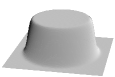
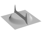
  Figure 2: Profiles of eigenlevel densities $R_{1}^{(\beta)}(z;n)$, plotted as functions of the complex energy $z=x+iy$ for $n$ fixed, show a nearly uniform eigenlevel distribution in GinUE (left panel), a depletion of eigenvalues along the real axis in GinSE as exemplified by the density drop at $y=0$ (middle panel), and accumulation of real eigenvalues in GinOE displayed as a wall at $y=0$ (right panel); the wall height imitates the density of real eigenvalues.

• GinSE: In accordance with (1.1cgho) – (1.1cghu), the exact result for the mean spectral density reads (Mehta and Srivastava 1966, Kanzieper 2002a)

  $$R_{1}^{(4)}(z;n)=2y\,e^{-(x^{2}+y^{2})}\,{\rm Im\,}\kappa_{n}^{(4)}(x+iy,x-iy)$$ (1.1cghaa)

  with $\kappa_{n}^{(4)}$ given by (1.1cghp). For a large-$n$ GinSE matrix and $z=x+iy$ fixed, it reduces to (Kanzieper, 2002a)

  $$R_{1}^{(4)}(z;n\gg 1)\simeq\frac{y}{\sqrt{2\pi}}\,e^{-2y^{2}}{\rm\,erfi}\big{(}y\sqrt{2}\big{)}.$$ (1.1cghab)

  Here, ${\rm erfi\,}(\phi)$ is the imaginary error function

  $${\rm erfi}(\phi)=\frac{2}{\sqrt{\pi}}\int_{0}^{\phi}dt\,e^{t^{2}}.$$

  Both results [(1.1cghaa) and (1.1cghab)] suggest that the mean eigenvalue density is no longer uniform but exhibits a depletion of eigenvalues along the real axis. Similarly to the GinUE, the mean spectral density in GinSE is suppressed away from a disk of the radius $\sqrt{2n}$ as suggested by the circular law

  $$\lim_{n\rightarrow\infty}R_{1}^{(4)}({\hat{z}}\sqrt{2n};n)=\frac{1}{2\pi}\left\{\begin{array}[]{cc}1&{\rm if\;}|{\hat{z}}|<1\\ 0&{\rm if\;}|{\hat{z}}|>1\\ \end{array}\right.$$ (1.1cghae)

  due to Khoruzhenko and Mezzadri (2005).
  

• GinOE: A mixed character of the GinOE spectrum consisting of both complex and real eigenvalues makes the RMT techniques based on the Dyson integration theorem inapplicable to the description of spectral statistical properties of GinOE.

  To evaluate the mean eigenvalue density in the finite-$n$ GinOE, a totally different approach has been invented by A. Edelman and co-workers (Edelman et al 1994, Edelman 1997). Starting directly with the definition (1.1cgha) taken at $\beta=1$ and applying the methods of multivariate statistical analysis (Muirhead 1982), these authors have separately determined the exact mean densities of purely real eigenvalues (Edelman et al 1994)

  $$R_{1,{\rm real}}^{(1)}(z;n)=\frac{\delta(y)}{\sqrt{2\pi}}\Bigg{[}\frac{\Gamma(n-1,x^{2})}{\Gamma(n-1)}+\frac{2^{n/2-3/2}}{\Gamma(n-1)}\,|x|^{n-1}\,e^{-x^{2}/2}\,\gamma\left(\frac{n-1}{2},\frac{x^{2}}{2}\right)\Bigg{]}$$

  and of strictly nonreal eigenvalues (Edelman 1997):

  $$R^{(1)}_{1,{\rm complex}}(z;n)=\sqrt{\frac{2}{\pi}}\,\frac{\Gamma(n-1,x^{2}+y^{2})}{\Gamma(n-1)}\,\,y\,e^{2y^{2}}\,{\rm erfc\,}\big{(}y\sqrt{2}\big{)}.$$ (1.1cghag)

  Here $x$ and $y$ are real and imaginary parts of $z=x+iy$. The function $\gamma(a,\phi)$ in (• ‣ 2.3) is the lower incomplete gamma function

  $$\gamma(a,\phi)=\int_{0}^{\phi}dt\,t^{a-1}e^{-t}.$$

  Importantly, no reference was made to the j.p.d.f. (1.1cghd) and (• ‣ 2.3) in deriving (• ‣ 2.3) and (1.1cghag).
  
  For a large-$n$ GinOE matrix and $z=x+iy$ fixed, the above two formulae yield the mean density of eigenvalues in the form

  $$R_{1}^{(1)}(z;n\gg 1)\simeq\frac{1}{\sqrt{2\pi}}\delta(y)+\sqrt{\frac{2}{\pi}}\,y\,e^{2y^{2}}\,{\rm erfc\,}\big{(}y\sqrt{2}\big{)}.$$ (1.1cghah)

  Similarly to GinUE and GinSE, the circular law (Girko 1984, Sommers et al 1988, Bai 1997, Edelman 1997)

  $$\lim_{n\rightarrow\infty}\,R_{1}^{(1)}({\hat{z}}\sqrt{n};n)=\frac{1}{\pi}\left\{\begin{array}[]{cc}1&{\rm if\;}|{\hat{z}}|<1\\ 0&{\rm if\;}|{\hat{z}}|>1\\ \end{array}\right.$$ (1.1cghak)

  holds.

2.4 Statistical description of the eigenvalue accumulation in GinOE

In essence, the approach culminating in the explicit formula (• ‣ 2.3) for the mean density of real eigenvalues represents the simplest possible quantitative description of the phenomenon of eigenvalue accumulation along the real axis. Complementarily, the one might be interested in the full statistics of the number ${\cal N}_{r}$ (${\cal N}_{c}$) of real (complex) eigenvalues occurring in the GinOE spectrum. In the latter context, the result (• ‣ 2.3) can only supply the first moment of ${\cal N}_{r}$ – the expected number $E_{n}={\mathbb{E}}[{\cal N}_{r}]$ of real eigenvalues. Indeed, integrating out the eigenlevel densities (• ‣ 2.3) and/or (1.1cghag) over the entire complex plane,

$$E_{n}=\int_{{\mathbb{C}}}d^{2}z\,R_{1,{\rm\,real}}^{(1)}(z;n)=n-\int_{{\mathbb{C}}\setminus{\mathbb{R}}}d^{2}z\,R_{1,{\rm\,complex}}^{(1)}(z;n),$$

Edelman et al (1994) have obtained the remarkable result

$$E_{n}=\frac{1}{2}+\sqrt{2}\,\frac{{}_{2}F_{1}\,(1,-1/2;n;1/2)}{B(n,1/2)}$$ (1.1cghal)

expressed in terms of the Gauss hypergeometric function and the Euler Beta function. As $n\rightarrow\infty$, it furnishes the asymptotic series

$$E_{n}=\sqrt{\frac{2n}{\pi}}\,\left(1-\frac{3}{8n}-\frac{3}{128n^{2}}+\frac{27}{1024n^{3}}+\frac{499}{32768n^{4}}+{\cal O}(n^{-5})\right)+\frac{1}{2}.$$ (1.1cgham)

The nonperturbative $\sqrt{n}$-dependence of leading term in (1.1cgham) had been earlier detected numerically by Sommers et al (1988).

What is about a more detailed statistical description of the number ${\cal N}_{r}$ (${\cal N}_{c}$) of real (complex) eigenvalues? Can all the moments and the entire probability function of the discrete random variable ${\cal N}_{r}$ (${\cal N}_{c}$) be determined? The preceding discussion, particularly highlighting a patchy knowledge of the spectral correlations in GinOE, suggests that both spectral characteristics, which can be expressed as

$${\mathbb{E}}[{\cal N}_{r}^{p}]=\sum_{k=1}^{p}S(p,k)\,\int_{{\mathbb{C}}}d^{2}z_{1}\cdots\int_{{\mathbb{C}}}d^{2}z_{k}\,R_{k,{\rm\,real}}^{(1)}(z_{1},\cdots,z_{k};n)$$ (1.1cghan)

and

$${\mathbb{E}}[{\cal N}_{c}^{p}]=\sum_{\ell=1}^{p}S(p,\ell)\,\int_{{\mathbb{C}}\setminus{\mathbb{R}}}d^{2}z_{1}\cdots\int_{{\mathbb{C}}\setminus{\mathbb{R}}}d^{2}z_{\ell}\,R_{\ell,{\rm\,complex}}^{(1)}(z_{1},\cdots,z_{\ell};n),$$ (1.1cghao)

are not within immediate reach. First, only one correlation function out of $p$ involved in either (1.1cghan) or (1.1cghao) is explicitly known. Second, even if all the multipoint correlation functions were readily available, the integrations in (1.1cghan) and (1.1cghao) would not be trivial either because of the anticipated inapplicability of the Dyson integration theorem as discussed in Section 2.3.

Some of the difficulties outlined here will be overcome in the present paper. For a list of our major results the reader is referred back to the Section 1.2. Proofs and derivations are given in the Sections to follow.

3 Statistics of real eigenvalues in GinOE spectra: A Pfaffian integral representation for the probability $p_{n,k}$

3.1 Generalities and known results

Instead of targeting the moments ${\mathbb{E}}[{\cal N}_{r}^{p}]$ of a fluctuating number of real eigenvalues as discussed in the previous section, we are going to directly determine the entire probability function $p_{n,k}={\rm Prob}({\cal N}_{r}=k)$. The definition of the $p_{n,k}$, describing the probability of finding exactly $k$ real eigenvalues in the spectrum of an $n\times n$ real Gaussian random matrix, can be deduced from (1.1cghd) and (• ‣ 2.3),

$$p_{n,k}={\rm Prob}({\boldsymbol{\cal H}}\in{\mathbb{T}}(n/k))=\prod_{i=1}^{k}\int_{{\mathbb{R}}}d\lambda_{i}\prod_{j=1}^{\ell}\int_{{\rm Im\,}z_{j}>0}d^{2}z_{j}\,P_{{\boldsymbol{\cal H}}\in{\mathbb{T}}(n/k)}.$$ (1.1cgha)

Here, $\ell$ is the number of pairs of complex conjugated eigenvalues in the spectrum of an $n\times n$ matrix ${\boldsymbol{\cal H}}\in{\mathbb{T}}(n/k)$ having exactly $k$ real eigenvalues, and $P_{{\boldsymbol{\cal H}}\in{\mathbb{T}}(n/k)}$ is the j.p.d.f. of all $n$ eigenvalues of such a matrix. Obviously, the identity $n=k+2\ell$ holds.

Previous attempts to determine the probability function $p_{n,k}$ based on (1.1cgha) brought no explicit formula for $p_{n,k}$ for generic $k$. The only analytic results available are due to Edelman (1997) who proved the following properties of the above probability function :

Property 1. The probability of having all $n$ eigenvalues real equals

$$p_{n,n}=2^{-n(n-1)/4}.$$ (1.1cghb)

Property 2. For all $0\leq k\leq n$, the $p_{n,k}$ are of the form

$$p_{n,k}=r_{n,k}+s_{n,k}\sqrt{2},$$ (1.1cghc)

where $r_{n,k}$ and $s_{n,k}$ are rational.

The first result is a simple consequence of (1.1cgha) which, at $k=n$, reduces to a known Selberg integral. All known examples suggest that this is the smallest probability out of all $p_{n,k}$’s. The second result is based on more involved considerations of (1.1cgha) and (1.1cghd).

3.2 Joint probability density function of complex eigenvalues of ${\boldsymbol{\cal H}}\in{\mathbb{T}}(n/k)$

To evaluate the sought probability function $p_{n,k}$, we start with the definition (1.1cgha). In a first step, we carry out the $\lambda$-integrations therein to assess the j.p.d.f. of all complex eigenvalues of a random matrix ${\boldsymbol{\cal H}}\in{\mathbb{T}}(n/k)$ having exactly $k$ real eigenvalues:

$$P_{{\boldsymbol{\cal H}_{k}}}(z_{1},\cdots,z_{\ell})=\prod_{i=1}^{k}\int_{{\mathbb{R}}}d\lambda_{i}\,P_{{\boldsymbol{\cal H}}\in{\mathbb{T}}(n/k)}(\lambda_{1},\cdots,\lambda_{k};z_{1},\cdots,z_{\ell}).$$ (1.1cghd)

To proceed, we consult (• ‣ 2.3) to spot that a part of it,

$${\cal I}_{k,\ell}(\{z,{\bar{z}}\})\equiv\prod_{i=1}^{k}\int_{{\mathbb{R}}}d\lambda_{i}\,\prod_{j=1}^{k}\,e^{-\lambda_{j}^{2}/2}\prod_{i>j}^{k}|\lambda_{i}-\lambda_{j}|\,\prod_{j=1}^{k}\prod_{i=1}^{\ell}(\lambda_{j}-z_{i})(\lambda_{j}-{\bar{z}}_{i}),$$ (1.1cghe)

coincides up to a prefactor to be specified below with the average characteristic polynomial

$${\cal P}_{k,\ell}(\{z,{\bar{z}}\})=\left(\int D{{\boldsymbol{\cal O}}}\,e^{-{\rm tr\,}{\boldsymbol{\cal O}}^{2}/2}\right)^{-1}$$

$$\times\int D{{\boldsymbol{\cal O}}}\prod_{j=1}^{\ell}{\rm det\,}(z_{j}-{\boldsymbol{\cal O}})\,{\rm det\,}({\bar{z}}_{j}-{\boldsymbol{\cal O}})\,e^{-{\rm tr\,}{\boldsymbol{\cal O}}^{2}/2}$$ (1.1cghf)

of a $k\times k$ real symmetric matrix ${\boldsymbol{\cal O}}={\boldsymbol{\cal O}}^{T}$ drawn from the GOE. More precisely,

$${\cal I}_{k,\ell}(\{z,{\bar{z}}\})={\mathfrak{s}}_{k}\,k!\,{\cal P}_{k,\ell}(\{z,{\bar{z}}\}),$$

where ${\mathfrak{s}}_{k}$ is given by the Selberg integral (Mehta 2004)

$${\mathfrak{s}}_{k}=\frac{1}{k!}\prod_{i=1}^{k}\int_{{\mathbb{R}}}d\lambda_{i}\,\prod_{j=1}^{k}\,e^{-\lambda_{j}^{2}/2}\prod_{i>j}^{k}|\lambda_{i}-\lambda_{j}|=2^{k/2}\,\prod_{j=1}^{k}\Gamma(j/2).$$ (1.1cghg)

Consequently, the j.p.d.f. of all complex eigenvalues of ${\boldsymbol{\cal H}}\in{\mathbb{T}}(n/k)$ is expressed in terms of the average GOE characteristic polynomial ${\cal P}_{k,\ell}(\{z,{\bar{z}}\})$ as

$$P_{{\boldsymbol{\cal H}_{k}}}(z_{1},\cdots,z_{\ell}) =\frac{2^{\ell}}{i^{\ell}\ell!}\,\frac{{\mathfrak{s}}_{k}}{{\mathfrak{s}}_{n}}\,p_{n,n}\;{\cal P}_{k,\ell}(\{z,{\bar{z}}\})\prod_{i>j=1}^{\ell}|z_{i}-z_{j}|^{2}|z_{i}-{\bar{z}}_{j}|^{2}\,$$ (1.1cghh)

$$\times\prod_{j=1}^{\ell}\,(z_{j}-{\bar{z}}_{j})\,{\rm erfc}\left(\frac{z_{j}-{\bar{z}}_{j}}{i\sqrt{2}}\right)\,\exp\left(-\frac{z_{j}^{2}+{\bar{z}}_{j}^{2}}{2}\right).$$

A little bit more spadework is needed to appreciate the beauty hidden in this representation. Borrowing the result due to Borodin and Strahov (2005), who discovered a Pfaffian formula for a general averaged GOE characteristic polynomial (see also an earlier paper by Nagao and Nishigaki (2001)), we may write ${\cal P}_{k,\ell}$ in the form

$${\cal P}_{k,\ell}(\{z,{\bar{z}}\})=\frac{{\mathfrak{s}}_{n}/{\mathfrak{s}}_{k}}{\Delta_{2\ell}(\{z,{\bar{z}}\})}\,(-1)^{\ell}$$

$$\times\prod_{j=1}^{\ell}\,\exp\left(\frac{z_{j}^{2}+{\bar{z}}_{j}^{2}}{2}\right)\,{\rm pf\,}\left[\begin{array}[]{cc}{\cal D}_{n}(z_{i},z_{j})&{\cal D}_{n}(z_{i},{\bar{z}}_{j})\\ {\cal D}_{n}({\bar{z}}_{i},z_{j})&{\cal D}_{n}({\bar{z}}_{i},{\bar{z}}_{j})\\ \end{array}\right]_{2\ell\times 2\ell}.$$ (1.1cghk)

Here, ${\cal D}_{n}(z_{i},z_{j})$ is the so-called $D$-part of the $2\times 2$ GOE matrix kernel (Tracy and Widom 1998) to be defined in (1.1cghp) and (1.1cghq) below; $\Delta_{2\ell}(\{z,{\bar{z}}\})$ is the Vandermonde determinant

$$\Delta_{2\ell}(\{z,{\bar{z}}\})=\Delta_{2\ell}(z_{1},{\bar{z}}_{1},\cdots,z_{\ell},{\bar{z}}_{\ell})=\prod_{i>j}^{\ell}|z_{i}-z_{j}|^{2}\,\prod_{i>j}^{\ell}|z_{i}-{\bar{z}}_{j}|^{2}\,\prod_{i=1}^{\ell}({\bar{z}}_{i}-z_{i}).$$ (1.1cghl)

Combining (1.1cghh), (3.2) and (1.1cghl), we obtain:

$$P_{{\boldsymbol{\cal H}_{k}}}(z_{1}\cdots,z_{\ell}) =\frac{p_{n,n}}{\ell!}\,\left(\frac{2}{i}\right)^{\ell}\,$$ (1.1cgho)

$$\times\prod_{j=1}^{\ell}\,{\rm erfc}\left(\frac{z_{j}-{\bar{z}}_{j}}{i\sqrt{2}}\right)\,{\rm pf\,}\left[\begin{array}[]{cc}{\cal D}_{n}(z_{i},z_{j})&{\cal D}_{n}(z_{i},{\bar{z}}_{j})\\ {\cal D}_{n}({\bar{z}}_{i},z_{j})&{\cal D}_{n}({\bar{z}}_{i},{\bar{z}}_{j})\\ \end{array}\right]_{2\ell\times 2\ell}$$

where $({\rm Re}\,z_{1},\cdots,{\rm Re}\,z_{\ell})\in{\mathbb{R}}^{\ell}$ and $({\rm Im}\,z_{1},\cdots,{\rm Im}\,z_{\ell})\in({\mathbb{R}}^{+})^{\ell}$ by derivation.

Equation (1.1cgho) is the central result of this section. Announced in (1.1cf), it describes the j.p.d.f. of $\ell$ pairs of complex conjugated eigenvalues $\{z_{j},{\bar{z}}_{j}\}$ of an $n\times n$ random matrix ${\boldsymbol{\cal H}}_{k}$ whose $k$ remaining eigenvalues are real, $k+2\ell=n$.

To make the expression for the j.p.d.f. $P_{{\boldsymbol{\cal H}}_{k}}$ explicit, we have to specify the kernel function ${\cal D}_{n}(z_{i},z_{j})$. The latter turns out to be sensitive to the parity of $n$ (see, e.g., Adler et al (2000)). For $n=2m$ even, the kernel function is given by

$${\cal D}_{2m}(x,y)=\frac{1}{2}e^{-(x^{2}+y^{2})/2}\sum_{j=0}^{m-1}\frac{q_{2j+1}(x)\,q_{2j}(y)-q_{2j}(x)\,q_{2j+1}(y)}{h_{j}}$$ (1.1cghp)

while for $n=2m+1$ odd, it equals

$${\cal D}_{2m+1}(x,y)=\frac{1}{2}e^{-(x^{2}+y^{2})/2}\sum_{j=0}^{m-1}\frac{{\tilde{q}}_{2j+1}(x)\,{\tilde{q}}_{2j}(y)-{\tilde{q}}_{2j}(x)\,{\tilde{q}}_{2j+1}(y)}{h_{j}}.$$ (1.1cghq)

Both representations (1.1cghp) and (1.1cghq) involve the polynomials $q_{j}(x)$ skew orthogonal on ${\mathbb{R}}$ with respect to the GOE skew product (Mehta 2004)

$$\left<f,\,g\right>=\frac{1}{2}\int_{{\mathbb{R}}}dx\,e^{-x^{2}/2}\int_{{\mathbb{R}}}dy\,e^{-y^{2}/2}{\rm sgn}(y-x)\,f(x)\,g(y)$$ (1.1cghr)

such that

$$\left<q_{2k},q_{2\ell+1}\right>=-\left<q_{2k+1},q_{2\ell}\right>=h_{k}\delta_{k,\ell},\;\;\;\left<q_{2k},q_{2\ell}\right>=\left<q_{2k+1},q_{2\ell+1}\right>=0.$$ (1.1cghs)

The skew orthogonal polynomials $q_{j}(x)$ can be expressed in terms of Hermite polynomials as

$$q_{2j}(x)=\frac{1}{2^{2j}}\,H_{2j}(x),$$

$$q_{2j+1}(x)=\frac{1}{2^{2j+1}}\,\big{[}H_{2j+1}(x)-4j\,H_{2j-1}(x)\big{]}$$ (1.1cght)

while “tilded” polynomials ${\tilde{q}}_{j}(x)$ entering (1.1cghq) are related to $q_{j}(x)$ via

$${\tilde{q}}_{2j}(x)=q_{2j}(x)-\frac{(2j)!}{2^{2j}j!}\,\frac{2^{2m}m!}{(2m)!}\,q_{2m}(x),$$

$${\tilde{q}}_{2j+1}(x)=q_{2j+1}(x).$$ (1.1cghu)

Specifying the normalisation

$$h_{j}=\left<q_{2j},\,q_{2j+1}\right>=\frac{\sqrt{\pi}\,(2j)!}{2^{2j}}$$ (1.1cghv)

completes our derivation of (1.1cgho).

3.3 Probability function $p_{n,k}$ as a Pfaffian integral and inapplicability of the Dyson integration theorem for its calculation

The results obtained in Section 3.2 allow us to express the probability function $p_{n,k}$ in the form of an $\ell$-fold integral

$$p_{n,k}=\frac{p_{n,n}}{\ell!}\,\left(\frac{2}{i}\right)^{\ell}\,\prod_{j=1}^{\ell}\int_{{\rm Im\,}z_{j}>0}d^{2}z_{j}\,$$

$$\times\;{\rm erfc}\left(\frac{z_{j}-{\bar{z}}_{j}}{i\sqrt{2}}\right)\,{\rm pf\,}\left[\begin{array}[]{cc}{\cal D}_{n}(z_{i},z_{j})&{\cal D}_{n}(z_{i},{\bar{z}}_{j})\\ {\cal D}_{n}({\bar{z}}_{i},z_{j})&{\cal D}_{n}({\bar{z}}_{i},{\bar{z}}_{j})\\ \end{array}\right]_{2\ell\times 2\ell}$$ (1.1cghy)

involving a Pfaffian. It can also be rewritten as a quaternion determinant

$${\rm pf\,}\left[\begin{array}[]{cc}{\cal D}_{n}(z_{i},z_{j})&{\cal D}_{n}(z_{i},{\bar{z}}_{j})\\ {\cal D}_{n}({\bar{z}}_{i},z_{j})&{\cal D}_{n}({\bar{z}}_{i},{\bar{z}}_{j})\\ \end{array}\right]_{2\ell\times 2\ell}={\rm qdet}[{\hat{\cal D}}_{n}(z_{i},z_{j})]_{\ell\times\ell}$$ (1.1cghab)

where the self-dual quaternion ${\hat{\cal D}}_{n}(z_{i},z_{j})$ has a $2\times 2$ matrix representation

$$\Theta[{\hat{\cal D}}_{n}(z_{i},z_{j})]=\left(\begin{array}[]{rr}-{\cal D}_{n}(\bar{z}_{i},z_{j})&-{\cal D}_{n}({\bar{z}}_{i},{\bar{z}}_{j})\\ {\cal D}_{n}(z_{i},z_{j})&{\cal D}_{n}(z_{i},{\bar{z}}_{j})\\ \end{array}\right).$$ (1.1cghae)

The Pfaffian/quaternion determinant form of the integrand in (3.3), closely resembling the structure of both the j.p.d.f. (1.1cghl) of all complex eigenvalues and the $p$-point correlation function (1.1cghu) in GinSE, makes it tempting to attack the $\ell$-fold integral (3.3) with the help of the Dyson integration theorem (see Section 2.3). Unfortunately, the key condition of this theorem – the projection property – is not fulfilled.

To see this point, we represent the kernel function ${\cal D}_{n}(x,y)$ in the form

$${\cal D}_{n}(x,y)=\frac{1}{2}\,e^{-(x^{2}+y^{2})/2}\sum_{j,k=0}^{n-1}q_{j}(x)\,{\hat{\mu}}_{jk}\,q_{k}(y),$$ (1.1cghaf)

see the primary definition (1.1cghp) and (1.1cghq). In (1.1cghaf), the real antisymmetric matrix ${\boldsymbol{\hat{\mu}}}$ of the size $n\times n$ depends on the parity of $n$. It equals

$${\hat{\mu}}^{\rm even}_{jk}=\left(\begin{array}[]{ccc}-{\boldsymbol{\hat{e}}}_{2}h_{0}^{-1}&{}\hfil&{}\hfil\\ {}\hfil&\ddots&{}\hfil\\ {}\hfil&{}\hfil&-{\boldsymbol{\hat{e}}}_{2}h_{m-1}^{-1}\\ \end{array}\right)$$ (1.1cghaj)

and

$${\hat{\mu}}^{\rm odd}_{jk}=\left(\begin{array}[]{cccc}-{\boldsymbol{\hat{e}}}_{2}h_{0}^{-1}&{}\hfil&{}\hfil&-{\boldsymbol{\hat{\varsigma}}}_{0}^{\rm T}\\ {}\hfil&\ddots&{}\hfil&\vdots\\ {}\hfil&{}\hfil&-{\boldsymbol{\hat{e}}}_{2}h_{m-1}^{-1}&-{\boldsymbol{\hat{\varsigma}}}_{m-1}^{\rm T}\\ {\boldsymbol{\hat{\varsigma}}}_{0}&\cdots&{\boldsymbol{\hat{\varsigma}}}_{m-1}&0\\ \end{array}\right)$$ (1.1cghao)

for $n=2m$ and $n=2m+1$, respectively. We remind that $h_{j}$ is defined by (1.1cghv); also we have used the notation

$${\boldsymbol{\hat{e}}}_{2}=\left(\begin{array}[]{cc}0&1\\ -1&0\\ \end{array}\right),\;\;\;{\boldsymbol{\hat{\varsigma}}}_{j}=c_{m}\,\big{(}0,\,\frac{1}{j!}\big{)},\;\;\;c_{m}=\frac{m!}{h_{m}}.$$ (1.1cghar)

Actually, the representation (1.1cghaf) can be put into a more general form due to Tracy and Widom (1998) that would contain arbitrary, not necessarily skew orthogonal, polynomials upon a proper redefinition of the matrix ${\boldsymbol{\hat{\mu}}}$.

For the Dyson integration theorem to be applicable, the projection property for the self-dual quaternion ${\hat{\cal D}}_{n}(z_{i},z_{j})$ must hold. For this to be the case, the integral identity

$$\int d\alpha(w)\,\left[{\cal D}_{n}(z_{1},w)\,{\cal D}_{n}({\bar{w}},z_{2})-{\cal D}_{n}(z_{2},w)\,{\cal D}_{n}({\bar{w}},z_{1})\right]\stackrel{{\scriptstyle?}}{{=}}-{\cal D}_{n}(z_{1},z_{2})$$ (1.1cghas)

should be satisfied for the measure

$$d\alpha(w)={\rm erfc}\,\left(\frac{w-{\bar{w}}}{i\sqrt{2}}\right)\theta({\rm Im\,}w)\,d^{2}w.$$ (1.1cghat)

Here, $\theta(\phi)$ is the Heaviside step function,

$$\theta(\phi)=\left\{\begin{array}[]{cc}1&{\rm if\;}\phi>0\\ 0&{\rm if\;}\phi<0\\ \end{array}\right..$$ (1.1cghaw)

Straightforward calculations based on (1.1cghaf) show that the integral on the l.h.s. of (1.1cghas) equals

$$\frac{1}{2}\,e^{-(z_{1}^{2}+z_{2}^{2})/2}\sum_{j,k=0}^{n-1}q_{j}(z_{1})\,(\boldsymbol{{\hat{\mu}}\,{\hat{\chi}}\,{\hat{\mu}}})_{jk}\,q_{k}(z_{2}),$$ (1.1cghax)

where $n\times n$ matrix $\boldsymbol{{\hat{\chi}}}$ has the entries

$${\hat{\chi}}_{jk}=\frac{1}{2}\int d\alpha(w)\,e^{-(w^{2}+{\bar{w}}^{2})/2}\left[q_{j}(w)\,q_{k}({\bar{w}})-q_{j}({\bar{w}})\,q_{k}(w)\right].$$ (1.1cghay)

Since $\boldsymbol{({\hat{\mu}}\,{\hat{\chi}})}\neq-{\boldsymbol{\hat{1}}}_{n}$, the l.h.s. of (1.1cghas) given by (1.1cghax) differs from the r.h.s. (1.1cghas). As a result, the kernel function ${\cal D}_{n}(z_{1},z_{2})$ does not satisfy the projection property . Consequently, the Dyson integration theorem is inapplicable for the calculation of $p_{n,k}$ in the form of the Pfaffian integral (3.3).

4 Probability function $p_{n,k}$: Sensing a structure through particular cases

Before turning to the derivation of the general formula for $p_{n,k}$ (see the results announced in Section 1.2), it is instructive to consider a few particular cases corresponding to low values of $\ell$, the number of pairs of complex conjugated eigenvalues. Below, the cases of $\ell=1,\,2$ and $3$ are treated explicitly.

4.1 What is the probability to find exactly one pair of complex conjugated eigenvalues?

As a first nontrivial application of the Pfaffian integral representation (3.3) for the probability function $p_{n,k}$, let us consider the next-to-the-simplest case of $\ell=1$ corresponding to the occurrence of exactly one pair of complex conjugated eigenvalues. Since the $D$-kernel (1.1cghaf) is antisymmetric under exchange of its arguments,

$${\cal D}_{n}(x,y)=-{\cal D}_{n}(y,x),$$ (1.1cgha)

the Pfaffian in (3.3) reduces to

$${\rm pf\,}\left[\begin{array}[]{cc}0&{\cal D}_{n}(z,{\bar{z}})\\ -{\cal D}_{n}(z,{\bar{z}})&0\\ \end{array}\right]={\cal D}_{n}(z,{\bar{z}})$$ (1.1cghd)

resulting in

$$p_{n,n-2}=p_{n,n}\,\frac{2}{i}\,\,\int_{{\rm Im\,}z>0}d^{2}z\,\,{\rm erfc}\left(\frac{z-{\bar{z}}}{i\sqrt{2}}\right)\,{\cal D}_{n}(z,{\bar{z}}).$$ (1.1cghe)

To calculate the integral

$${\cal I}_{1}=\int_{{\rm Im\,}z>0}d^{2}z\,\,{\rm erfc}\left(\frac{z-{\bar{z}}}{i\sqrt{2}}\right)\,{\cal D}_{n}(z,{\bar{z}})=\int d\alpha(z)\,{\cal D}_{n}(z,{\bar{z}})$$

(see (1.1cghat)), we rewrite it in a more symmetric manner

$$\frac{1}{2}\,\int d\alpha(z)\,\Big{[}{\cal D}_{n}(z,{\bar{z}})-{\cal D}_{n}({\bar{z}},z)\Big{]},$$

and make use of (1.1cghay), (1.1cghat) and (1.1cghaf) to deduce that it equals

$$-\frac{1}{2}\,\sum_{j,k=0}^{n-1}\mu_{jk}\chi_{kj}=-\frac{1}{2}{\rm tr}_{(0,n-1)}({\boldsymbol{{\hat{\mu}}{\hat{\chi}}}}),$$

or, equivalently,

$${\cal I}_{1}=\int d\alpha(z)\,{\cal D}_{n}(z,{\bar{z}})=\frac{i}{4}\,{\rm tr}_{(0,n-1)}{\boldsymbol{\hat{\sigma}}}.$$ (1.1cghf)

Here, ${\boldsymbol{\hat{\sigma}}}$ is given by ${\boldsymbol{\hat{\sigma}}}=2i{\boldsymbol{{\hat{\mu}}{\hat{\chi}}}}$ (see also Appendix B). We therefore conclude that the probability sought equals

$$p_{n,n-2}=\frac{1}{2}\,p_{n,n}\,{\rm tr}_{(0,n-1)}{\boldsymbol{\hat{\sigma}}}.$$ (1.1cghg)

Due to the trace identity (C.5) proven in Appendix C, we eventually derive:

$$p_{n,n-2}=p_{n,n}\,{\rm tr}_{(0,\lfloor n/2\rfloor-1)}{\boldsymbol{\hat{\varrho}}},$$ (1.1cghh)

reducing the size of the matrix by two. Here, the smaller matrix ${\boldsymbol{\hat{\varrho}}}$ depends on the parity of $n$, as defined in the Section 1.2 (see also (C.3) and (C.4)).

Remarkably, the trace in (1.1cghh) can explicitly be calculated (see Appendix D) to yield a closed expression for the probability to find exactly one pair of complex conjugated eigenvalues:

$$p_{n,n-2}=2\,p_{n,n}\,\int_{0}^{\infty}dy\,y\,e^{y^{2}}\,{\rm erfc}(y\sqrt{2})\,L_{n-2}^{2}(-2y^{2}).$$ (1.1cghi)

Yet another, though equivalent, representation for the probability $p_{n,n-2}$ is given in Section 7 that addresses the large-$n$ behaviour of $p_{n,n-2}$.

4.2 Two pairs of complex conjugated eigenvalues ($\ell=2$)

For $\ell=2$, the Pfaffian in (3.3)

$${\rm pf\,}\left[\begin{array}[]{cccc}0&{\cal D}_{n}(z_{1},{\bar{z}}_{1})&{\cal D}_{n}(z_{1},z_{2})&{\cal D}_{n}(z_{1},{\bar{z}}_{2})\\ -{\cal D}_{n}(z_{1},{\bar{z}}_{1})&0&{\cal D}_{n}({\bar{z}}_{1},z_{2})&{\cal D}_{n}({\bar{z}}_{1},{\bar{z}}_{2})\\ -{\cal D}_{n}(z_{1},z_{2})&-{\cal D}_{n}({\bar{z}}_{1},z_{2})&0&{\cal D}_{n}(z_{2},{\bar{z}}_{2})\\ -{\cal D}_{n}(z_{1},{\bar{z}}_{2})&-{\cal D}_{n}({\bar{z}}_{1},{\bar{z}}_{2})&-{\cal D}_{n}(z_{2},{\bar{z}}_{2})&0\\ \end{array}\right]$$ (1.1cghn)

reduces to

$${\cal D}_{n}(z_{1},{\bar{z}}_{1})\,{\cal D}_{n}(z_{2},{\bar{z}}_{2})+{\cal D}_{n}(z_{1},{\bar{z}}_{2})\,{\cal D}_{n}({\bar{z}}_{1},z_{2})-{\cal D}_{n}(z_{1},z_{2})\,{\cal D}_{n}({\bar{z}}_{1},{\bar{z}}_{2}),$$ (1.1cgho)

so that

$$p_{n,n-4} =-2\,p_{n,n}\,\int d\alpha(z_{1})\,\int d\alpha(z_{2})\,$$ (1.1cghp)

$$\times\Big{[}{\cal D}_{n}(z_{1},{\bar{z}}_{1})\,{\cal D}_{n}(z_{2},{\bar{z}}_{2})+{\cal D}_{n}(z_{1},{\bar{z}}_{2})\,{\cal D}_{n}({\bar{z}}_{1},z_{2})-{\cal D}_{n}(z_{1},z_{2})\,{\cal D}_{n}({\bar{z}}_{1},{\bar{z}}_{2})\Big{]}.$$

Apart from a known integral taking the form of (1.1cghf), a new integral

$${\cal I}_{2}=\int d\alpha(z_{1})\,\int d\alpha(z_{2})\,\Big{[}{\cal D}_{n}(z_{1},{\bar{z}}_{2})\,{\cal D}_{n}({\bar{z}}_{1},z_{2})-{\cal D}_{n}(z_{1},z_{2})\,{\cal D}_{n}({\bar{z}}_{1},{\bar{z}}_{2})\Big{]}$$ (1.1cghq)

appears in (1.1cghp). Somewhat lengthy but straightforward calculations based on (1.1cghay), (1.1cghat) and (1.1cghaf) result in

$${\cal I}_{2}=\frac{1}{8}\,{\rm tr}_{(0,n-1)}({\boldsymbol{\hat{\sigma}}}^{2}).$$ (1.1cghr)

Combining (1.1cghp), (1.1cghf), (1.1cghq) and (1.1cghr), we obtain:

$$p_{n,n-4}=p_{n,n}\,\left[\frac{1}{8}\,\left({\rm tr}_{(0,n-1)}{\boldsymbol{\hat{\sigma}}}\right)^{2}-\frac{1}{4}\,{\rm tr}_{(0,n-1)}({\boldsymbol{\hat{\sigma}}}^{2})\right].$$ (1.1cghs)

Due to the trace identity (C.5) proven in Appendix C, the latter reduces to

$$p_{n,n-4}=\frac{1}{2}\,p_{n,n}\,\left[\left({\rm tr}_{(0,\lfloor n/2\rfloor-1)}{\boldsymbol{\hat{\varrho}}}\right)^{2}-{\rm tr}_{(0,\lfloor n/2\rfloor-1)}({\boldsymbol{\hat{\varrho}}}^{2})\right].$$ (1.1cght)

Interestingly, the expression in the parenthesis of (1.1cght) coincides with $Z_{(1^{2})}(p_{1},p_{2})$ after the substitution ${\rm tr\,}{\boldsymbol{\hat{\varrho}}}^{j}=p_{j}$ (see Table 1).

4.3 Three pairs of complex conjugated eigenvalues ($\ell=3$)

The complexity of the integrand in (3.3) grows rapidly with increasing $\ell$. For $\ell=3$, that is three pairs of complex conjugated eigenvalues in the matrix spectrum, the Pfaffian of the $6\times 6$ antisymmetric matrix

$$\left(\begin{array}[]{cccccc}0&{\cal D}_{n}(z_{1},{\bar{z}}_{1})&{\cal D}_{n}(z_{1},z_{2})&{\cal D}_{n}(z_{1},{\bar{z}}_{2})&{\cal D}_{n}(z_{1},z_{3})&{\cal D}_{n}(z_{1},{\bar{z}}_{3})\\ -{\cal D}_{n}(z_{1},{\bar{z}}_{1})&0&{\cal D}_{n}({\bar{z}}_{1},z_{2})&{\cal D}_{n}({\bar{z}}_{1},{\bar{z}}_{2})&{\cal D}_{n}({\bar{z}}_{1},z_{3})&{\cal D}_{n}({\bar{z}}_{1},{\bar{z}}_{3})\\ -{\cal D}_{n}(z_{1},z_{2})&-{\cal D}_{n}({\bar{z}}_{1},z_{2})&0&{\cal D}_{n}(z_{2},{\bar{z}}_{2})&{\cal D}_{n}(z_{2},z_{3})&{\cal D}_{n}(z_{2},{\bar{z}}_{3})\\ -{\cal D}_{n}(z_{1},{\bar{z}}_{2})&-{\cal D}_{n}({\bar{z}}_{1},{\bar{z}}_{2})&-{\cal D}_{n}(z_{2},{\bar{z}}_{2})&0&{\cal D}_{n}({\bar{z}}_{2},z_{3})&{\cal D}_{n}({\bar{z}}_{2},{\bar{z}}_{3})\\ -{\cal D}_{n}(z_{1},z_{3})&-{\cal D}_{n}({\bar{z}}_{1},z_{3})&-{\cal D}_{n}(z_{2},z_{3})&-{\cal D}_{n}({\bar{z}}_{2},z_{3})&0&{\cal D}_{n}(z_{3},{\bar{z}}_{3})\\ -{\cal D}_{n}(z_{1},{\bar{z}}_{3})&-{\cal D}_{n}({\bar{z}}_{1},{\bar{z}}_{3})&-{\cal D}_{n}(z_{2},{\bar{z}}_{3})&-{\cal D}_{n}({\bar{z}}_{2},{\bar{z}}_{3})&-{\cal D}_{n}(z_{3},{\bar{z}}_{3})&0\\ \end{array}\right)$$ (1.1cghaa)

is getting involved. It can be calculated with some effort to give $15$ terms which can be attributed to three different groups. The first group consists of the single term

$$G_{1}={\cal D}_{n}(z_{1},{\bar{z}}_{1})\,{\cal D}_{n}(z_{2},{\bar{z}}_{2})\,{\cal D}_{n}(z_{3},{\bar{z}}_{3}).$$ (1.1cghab)

The second group contains $6$ terms,

$$G_{2} ={\cal D}_{n}(z_{1},{\bar{z}}_{1})\,\Big{[}{\cal D}_{n}(z_{2},{\bar{z}}_{3})\,{\cal D}_{n}({\bar{z}}_{2},z_{3})\,-{\cal D}_{n}(z_{2},z_{3})\,{\cal D}_{n}({\bar{z}}_{2},{\bar{z}}_{3})\Big{]}\,$$ (1.1cghac)

$$+{\cal D}_{n}(z_{2},{\bar{z}}_{2})\,\Big{[}{\cal D}_{n}(z_{1},{\bar{z}}_{3})\,{\cal D}_{n}({\bar{z}}_{1},z_{3})\,-{\cal D}_{n}(z_{1},z_{3})\,{\cal D}_{n}({\bar{z}}_{1},{\bar{z}}_{3})\Big{]}\,$$

$$+{\cal D}_{n}(z_{3},{\bar{z}}_{3})\,\Big{[}{\cal D}_{n}(z_{1},{\bar{z}}_{2})\,{\cal D}_{n}({\bar{z}}_{1},z_{2})\,-{\cal D}_{n}(z_{1},z_{2})\,{\cal D}_{n}({\bar{z}}_{1},{\bar{z}}_{2})\Big{]},$$

while the third group counts $8$ terms:

$$G_{3} ={\cal D}_{n}(z_{1},{\bar{z}}_{3})\,{\cal D}_{n}({\bar{z}}_{2},z_{3})\,{\cal D}_{n}({\bar{z}}_{1},z_{2})\,-{\cal D}_{n}({\bar{z}}_{1},z_{3})\,{\cal D}_{n}(z_{2},{\bar{z}}_{3})\,{\cal D}_{n}(z_{1},{\bar{z}}_{2})\,$$ (1.1cghad)

$$+{\cal D}_{n}(z_{1},{\bar{z}}_{2})\,{\cal D}_{n}(z_{2},z_{3})\,{\cal D}_{n}({\bar{z}}_{1},{\bar{z}}_{3})-{\cal D}_{n}({\bar{z}}_{1},z_{2})\,{\cal D}_{n}({\bar{z}}_{2},{\bar{z}}_{3})\,{\cal D}_{n}(z_{1},z_{3})\,$$

$$+{\cal D}_{n}({\bar{z}}_{1},{\bar{z}}_{2})\,{\cal D}_{n}(z_{2},{\bar{z}}_{3})\,{\cal D}_{n}(z_{1},z_{3})\,-{\cal D}_{n}(z_{1},z_{2})\,{\cal D}_{n}({\bar{z}}_{2},z_{3})\,{\cal D}_{n}({\bar{z}}_{1},{\bar{z}}_{3})\,$$

$$+{\cal D}_{n}(z_{1},z_{2})\,{\cal D}_{n}({\bar{z}}_{2},{\bar{z}}_{3})\,{\cal D}_{n}({\bar{z}}_{1},z_{3})-{\cal D}_{n}({\bar{z}}_{1},{\bar{z}}_{2})\,{\cal D}_{n}(z_{2},z_{3})\,{\cal D}_{n}(z_{1},{\bar{z}}_{3}).$$

In the above notation, the probability function $p_{n,n-6}$ takes the form

$${}p_{n,n-6}=\frac{4i}{3}\,p_{n,n}\,\int d\alpha(z_{1})\,\int d\alpha(z_{2})\,\int d\alpha(z_{3})\,\Big{[}G_{1}+G_{2}+G_{3}\Big{]}.$$ (1.1cghae)

The integrals containing $G_{1}$ and $G_{2}$ can easily be performed with the help of (1.1cghf), (1.1cghq) and (1.1cghr) to bring

$$\int d\alpha(z_{1})\,\int d\alpha(z_{2})\,\int d\alpha(z_{3})\,G_{1}={\cal I}_{1}^{3}=\left(\frac{i}{4}\,{\rm tr}_{(0,n-1)}{\boldsymbol{\hat{\sigma}}}\right)^{3}$$ (1.1cghaf)

and

$$\int d\alpha(z_{1})\,\int d\alpha(z_{2})\,\int d\alpha(z_{3})\,G_{2} =3\,{\cal I}_{1}\,{\cal I}_{2}$$ (1.1cghag)

$$=3\,\left(\frac{i}{4}\,{\rm tr}_{(0,n-1)}{\boldsymbol{\hat{\sigma}}}\right)\,\left(\frac{1}{8}\,{\rm tr}_{(0,n-1)}({\boldsymbol{\hat{\sigma}}}^{2})\right).$$

The remaining integral involving $G_{3}$ can be evaluated similarly to ${\cal I}_{1}$ and ${\cal I}_{2}$, the result being

$${\cal I}_{3}=\int d\alpha(z_{1})\,\int d\alpha(z_{2})\,\int d\alpha(z_{3})\,G_{3}=\frac{i^{3}}{8}\,{\rm tr}_{(0,n-1)}({\boldsymbol{\hat{\sigma}}}^{3}).$$ (1.1cghah)

Combining (1.1cghae), (1.1cghaf), (1.1cghag) and (1.1cghah), we derive:

$$p_{n,n-6}=p_{n,n}\,\left[\frac{1}{48}\,\left({\rm tr}_{(0,n-1)}{\boldsymbol{\hat{\sigma}}}\right)^{3}-\frac{1}{8}\,{\rm tr}_{(0,n-1)}{\boldsymbol{\hat{\sigma}}}\,{\rm tr}_{(0,n-1)}({\boldsymbol{\hat{\sigma}}}^{2})+\frac{1}{6}\,{\rm tr}_{(0,n-1)}({\boldsymbol{\hat{\sigma}}}^{3})\right].$$

Finally, we apply the trace identity (C.5) to end up with the formula

$$p_{n,n-6} =\frac{1}{6}\,p_{n,n}\,\Big{[}\left({\rm tr}_{(0,\lfloor n/2\rfloor-1)}{\boldsymbol{\hat{\varrho}}}\right)^{3}$$ (1.1cghaj)

$$-3\,{\rm tr}_{(0,\lfloor n/2\rfloor-1)}{\boldsymbol{\hat{\varrho}}}\,{\rm tr}_{(0,\lfloor n/2\rfloor-1)}({\boldsymbol{\hat{\varrho}}}^{2})+2\,{\rm tr}_{(0,\lfloor n/2\rfloor-1)}({\boldsymbol{\hat{\varrho}}}^{3})\Big{]}.$$

The expression in the parenthesis of (1.1cghaj) is seen to coincide with $Z_{(1^{3})}(p_{1},p_{2},p_{3})$ after the substitution ${\rm tr\,}{\boldsymbol{\hat{\varrho}}}^{j}=p_{j}$ (see Table 1).

4.4 Higher $\ell$

The three examples considered clearly demonstrate that the calculational complexity grows enormously with increasing $\ell$, the number of complex conjugated eigenvalues in the random matrix spectrum. Indeed, the number of terms ${\cal N}_{\ell}$ in the expansion of the Pfaffian in (3.3) equals ${\cal N}_{\ell}=(2\ell-1)!!$ and exhibits a faster-than-exponential growth, ${\cal N}_{\ell}\approx 2^{\ell+1/2}\,e^{\ell\,(\ln\ell-1)}$, for $\ell\gg 1$. For this reason, one has to invent a classification of the terms arising in the Pfaffian expansion that facilitates their effective computation. This will be done in Section 5, where we introduce a topological interpretation of the Pfaffian expansion, and prove the Pfaffian integration theorem which can be viewed as a generalisation of the Dyson integration theorem (see Section 2.3).

5 Topological interpretation of the Pfaffian expansion, and the Pfaffian integration theorem

5.1 Statement of the main result and its discussion

Before stating the main result of this section, the Pfaffian integration theorem, we wish to start with presenting a simple Corollary to the Dyson integration theorem.
Corollary 5.1. Let $f(x,y)$ be a function with real, complex or quaternion values satisfying the conditions (1.1cghha) and (1.1cghhb) of the Theorem 2.1, and $d\pi$ be a suitable measure. Then

$$\int\prod_{j=1}^{\ell}d\pi(x_{j})\,{\rm det\,}[f(x_{i},x_{j})]_{\ell\times\ell}=\frac{\Gamma(c+1)}{\Gamma(c+1-\ell)},$$ (1.1cghaa)

where

$$c=\int d\pi(x)\,f(x,x).$$ (1.1cghab)

For $f$ taking quaternion values, the ${\rm det}$ should be interpreted as ${\rm qdet}$, the quaternion determinant (Dyson 1972).

Proof. Repeatedly apply the Dyson integration theorem to the l.h.s. of (1.1cghaa) to arrive at its r.h.s. $\;\;\;\blacksquare$

Importantly, the above Corollary exclusively applies to functions $f(x,y)$ satisfying the projection property as defined in Section 2.3 (see Definition 2.1 therein). However, guided by our study of the integrable structure of GinOE, we are going to ask if the integrals of the kind (1.1cghaa) can explicitly be calculated if the projection property is relaxed. In general, the answer is positive. In particular, for $f(x,y)$ being a self-dual quaternion, the following integration theorem will be proven.
Theorem 5.1 (Pfaffian integration theorem). Let $d\pi(z)$ be any benign measure on $z\in{\mathbb{C}}$, and the function $Q_{n}(x,y)$ be an antisymmetric function of the form

$$Q_{n}(x,y)=\frac{1}{2}\sum_{j,k=0}^{n-1}q_{j}(x)\,{\hat{\mu}}_{jk}\,q_{k}(y)$$ (1.1cghba)

where the $$q_{j}(x) j {\boldsymbol{\hat{\mu}}}$$ are arbitrary polynomials of -th order, and is an antisymmetric matrix. Then the integration formula

$$\int_{{\mathbb{C}}}\,\prod_{j=1}^{\ell}\,d\pi(z_{j})\,\,{\rm pf\,}\left[\begin{array}[]{cc}Q_{n}(z_{i},z_{j})&Q_{n}(z_{i},{\bar{z}}_{j})\\ Q_{n}({\bar{z}}_{i},z_{j})&Q_{n}({\bar{z}}_{i},{\bar{z}}_{j})\\ \end{array}\right]_{2\ell\times 2\ell}$$ (1.1cghbd)

$$=\left(\frac{i}{2}\right)^{\ell}Z_{(1^{\ell})}\left(\frac{1}{2}{\rm tr}_{(0,n-1)}{\boldsymbol{\hat{\upsilon}}}^{1},\cdots,\frac{1}{2}{\rm tr}_{(0,n-1)}{\boldsymbol{\hat{\upsilon}}}^{\ell}\right)$$ (1.1cghbe)

holds, provided the integrals in its l.h.s. exist. Here, $$Z_{(1^{\ell})} \ell {\boldsymbol{\hat{\upsilon}}}$$ are zonal polynomials whose arguments are determined by a matrix with the entries

$${\hat{\upsilon}}_{\alpha,\beta}=i\sum_{k=0}^{n-1}{\hat{\mu}}_{\alpha,k}\int_{z\in{\mathbb{C}}}d\pi(z)\left[q_{k}(z)\,q_{\beta}({\bar{z}})-q_{\beta}(z)\,q_{k}({\bar{z}})\right].$$ (1.1cghbf)

As we integrate over all variables, the Pfaffian integration theorem can be viewed as a generalisation of the Corollary 5.1 proven a few lines above, for the case of a kernel not satisfying the projection property. This follows from the identity

$${\rm pf\,}\left[\begin{array}[]{cc}Q_{n}(z_{i},z_{j})&Q_{n}(z_{i},{\bar{z}}_{j})\\ Q_{n}({\bar{z}}_{i},z_{j})&Q_{n}({\bar{z}}_{i},{\bar{z}}_{j})\\ \end{array}\right]_{2\ell\times 2\ell}={\rm qdet\,}\left[{\hat{Q}}_{n}(z_{i},z_{j})\right]_{\ell\times\ell},$$ (1.1cghk)

where the quaternion ${\hat{Q}}_{n}(z_{i},z_{j})$ has the $2\times 2$ matrix representation:

$$f(z_{i},z_{j})=\Theta[{\hat{Q}}_{n}(z_{i},z_{j})]=\left(\begin{array}[]{rr}-Q_{n}(\bar{z}_{i},z_{j})&-Q_{n}({\bar{z}}_{i},{\bar{z}}_{j})\\ Q_{n}(z_{i},z_{j})&Q_{n}(z_{i},{\bar{z}}_{j})\\ \end{array}\right).$$ (1.1cghn)

To see that the Pfaffian integration theorem reduces to the Corollary for the particular case of a kernel with restored projection property, we spot that the latter is equivalent to the statement

$${\boldsymbol{\hat{\upsilon}}}=-2i\,{\boldsymbol{\hat{1}}}_{n}$$ (1.1cgho)

as can be deduced from the discussion below (1.1cghas), Section 3.3. As a result,

$${\rm tr\,}_{(0,n-1)}\,{\boldsymbol{\hat{\upsilon}}\,}^{j}=n\,\left(\frac{2}{i}\right)^{\,j},$$ (1.1cghp)

and the r.h.s. of (1.1cghbd) reduces to (Macdonald 1998)

$$\left(\frac{i}{2}\right)^{\ell}Z_{(1^{\ell})}\left(\frac{n}{2}\,\left(\frac{2}{i}\right)^{1},\cdots,\frac{n}{2}\,\left(\frac{2}{i}\right)^{\ell}\right)=\left(\frac{i}{2}\frac{\partial}{\partial z}\right)^{\ell}\,\exp\Bigg{(}\frac{n}{2}\sum_{r\geq 1}(-1)^{r-1}\frac{(-2i\,z)^{r}}{r}\Bigg{)}\Bigg{|}_{z=0}$$

$$=\left(\frac{\partial}{\partial z}\right)^{\ell}(1+z)^{n/2}\Bigg{|}_{z=0}=\frac{\Gamma(n/2+1)}{\Gamma(n/2+1-\ell)}.$$ (1.1cghq)

Finally, noticing from (1.1cghn) that

$$\int\,d\pi(z)f(z,z)=\int\,d\pi(z)\,\left(\begin{array}[]{rr}Q_{n}(z,\bar{z})&0\\ 0&Q_{n}(z,{\bar{z}})\\ \end{array}\right)$$ (1.1cght)

$$=\frac{i}{4}\,{\boldsymbol{\hat{e}}_{0}}\,{\rm tr\,}_{(0,n-1)}{\boldsymbol{\hat{\upsilon}}}=(n/2)\,{\boldsymbol{\hat{e}}_{0}}$$ (1.1cghu)

with ${\boldsymbol{\hat{e}}_{0}}={\rm diag}(1,1)$, we conclude that the constant $c$ in the Corollary [(1.1cghab)] equals $c=n/2$ so that the result (5.1) brought by the Pfaffian integration theorem is identically equivalent to the one [(1.1cghaa)] following from the Dyson integration theorem. We stress that this is only true for the kernel $Q_{n}(z_{i},z_{j})$ satisfying the projection property.

To prove the Theorem 5.1, we will invent a formalism based on a topological interpretation of the ordered Pfaffian expansion. For the readers’ benefit, a vocabulary of the topological terms to be defined and used in the following sections is summarised in Table 3.

5.2 Topological interpretation of the ordered Pfaffian expansion

Table 3: The vocabulary of topological terms defined to interpret the ordered Pfaffian expansion. The notation used is: D – Definition, E – Example, L – Lemma, T – Theorem, C – Corollary, F – Figure.

• Term	Notation	Appearance
  String	${\cal S}_{i}$	D5.1, E5.1, F3, F4
  Length of a string	$\|{\cal S}_{i}\|$	D5.2, E5.2
  Equivalent strings	${\cal S}_{i}\sim{\cal S}_{j}$	D5.3, E5.3, L5.1, F3
  Equivalence class of strings	${\cal C}_{j}$	D5.4, E5.4, L5.1, F3, F5
  Size of equivalence class	$\|{\cal C}_{j}\|$	D5.4, L5.1, F3
  Substring	${\cal S}_{i}^{(p)}$	D5.5, E5.5
  Length of a substring	$p=\|{\cal S}_{i}^{(p)}\|$	D5.5, E5.5
  Loop-like substring	${\cal S}_{i}^{(p)}$	D5.6, E5.6, L5.2, L5.5,
  		F3, F4
  Longest loop-like string	${\cal S}_{i}^{(\ell)}$	F3, E5.7, L5.4
  Adjacent loop-like string	${\cal S}_{i}^{(p)}$	D5.7, E5.7, E5.9, E5.11,
  		L5.4–L5.6, C5.2, F4, F5
  Handedness of adjacent (sub)string	${\mathbb{H}}(\alpha_{L},\alpha_{R})$	D5.8, E5.8, E5.9, E5.11,
  		L5.6, C5.2, F5
  Equivalent adjacent (sub)strings	${\cal S}_{i}\sim{\cal S}_{j}$	D5.9, E5.10, E5.11,
  		L5.7, F5
  Equivalence class of adjacent (sub)strings	${\cal AC}_{j}$	D5.10
  Compound string	${\cal S}_{i}$	D5.11, T5.3, F3, F6
  Topology class	${\boldsymbol{\lambda}}$	F6

To integrate the Pfaffian in (1.1cghbd), we start with its ordered expansion

$${\rm pf\,}\left[\begin{array}[]{cc}Q_{n}(z_{i},z_{j})&Q_{n}(z_{i},{\bar{z}}_{j})\\ Q_{n}({\bar{z}}_{i},z_{j})&Q_{n}({\bar{z}}_{i},{\bar{z}}_{j})\\ \end{array}\right]_{2\ell\times 2\ell}=\frac{1}{2^{\ell}\ell!}\sum_{\sigma\in S_{2\ell}}{\rm sgn}(\sigma)\,\prod_{j=0}^{\ell-1}Q_{n}(w_{\sigma(2j+1)},w_{\sigma(2j+2)}).$$ (1.1cghx)

Here, the summation extends over all permutations $\sigma\in S_{2\ell}$ of $2\ell$ objects

$$\{w_{1}=z_{1},w_{2}={\bar{z}}_{1},\cdots,w_{2\ell-1}=z_{\ell},w_{2\ell}={\bar{z}}_{\ell}\}$$ (1.1cghz)

so that the total number of terms in (1.1cghx) is $(2\ell)!$.

5.2.1 Strings and their equivalence classes

Definition 5.1. Each term of the ordered Pfaffian expansion is called a string. The $i$-th string ${\cal S}_{i}$ equals

$${\cal S}_{i}={\rm sgn}(\sigma_{i})\,\prod_{j=0}^{\ell-1}Q_{n}(w_{\sigma_{i}(2j+1)},w_{\sigma_{i}(2j+2)}).$$ (1.1cghaa)

where $\sigma_{i}$ is the $i$-th permutation out of $(2\ell)!$ possible permutations $\sigma\in S_{2\ell}$. Notice that a sign is attached to each string.

Example 5.1. The ordered expansion of the Pfaffian for $\ell=2$ [see (1.1cghn)] contains $4!=24$ strings that we assign to three different groups (their meaning will become clear below):

$$\begin{array}[]{ccc}{}\hfil&{}\hfil&{}\hfil\\ \shadowbox{Group 1}&\shadowbox{Group 2}&\shadowbox{Group 3}\\ {}\hfil&{}\hfil&{}\hfil\\ ~{}~{}{\bf+(1{\bar{1}})(2{\bar{2}}){}{}}&~{}~{}{\bf+(1{\bar{2}})({\bar{1}}2){}{}}&~{}~{}{\bf-(12)({\bar{1}}{\bar{2}}){}{}}\\ -(1{\bar{1}})({\bar{2}}2)&-(1{\bar{2}})(2{\bar{1}})&+(12)({\bar{2}}{\bar{1}})\\ +({\bar{1}}1)({\bar{2}}2)&+({\bar{2}}1)(2{\bar{1}})&-(21)({\bar{2}}{\bar{1}})\\ -({\bar{1}}1)(2{\bar{2}})&-({\bar{2}}1)({\bar{1}}2)&+(21)({\bar{1}}{\bar{2}})\\ +(2{\bar{2}})(1{\bar{1}})&+({\bar{1}}2)(1{\bar{2}})&-({\bar{1}}{\bar{2}})(12)\\ -(2{\bar{2}})({\bar{1}}1)&-({\bar{1}}2)({\bar{2}}1)&+({\bar{1}}{\bar{2}})(21)\\ +({\bar{2}}2)({\bar{1}}1)&+(2{\bar{1}})({\bar{2}}1)&-({\bar{2}}{\bar{1}})(21)\\ -({\bar{2}}2)(1{\bar{1}})&-(2{\bar{1}})(1{\bar{2}})&+({\bar{2}}{\bar{1}})(12)\\ {}\hfil&{}\hfil&{}\hfil\\ \end{array}$$ (1.1cghan)

For brevity, the obvious notation $\pm(pq)({\bar{p}}{\bar{q}})$ was used to denote the string $\pm Q_{n}(z_{p},z_{q})Q_{n}({\bar{z}}_{p},{\bar{z}}_{q})$. The three strings shown in bold are those that previously appeared in (1.1cgho) when treating the probability $p_{n,n-4}$.

Definition 5.2. The length $\|{\cal S}_{i}\|$ of a string ${\cal S}_{i}$ equals the number of kernels it is composed of.

Example 5.2. The string ${\cal S}_{i}$ in (1.1cghaa) is of the length $\ell$: $\|{\cal S}_{i}\|=\ell$. All strings in (1.1cghan) are of the length $2$.

Definition 5.3. Two strings ${\cal S}_{i}$ and ${\cal S}_{j}$ of the ordered Pfaffian expansion are said to be equivalent strings, ${\cal S}_{i}\sim{\cal S}_{j}$, if they can be obtained from each other by (i) permutation of kernels and/or (ii) permutation of arguments inside kernels (these will also be called intra-kernel permutations).

Example 5.3. For $\ell=2$, three different groups of equivalent strings can be identified as suggested by (1.1cghan). The first group, exemplified by the string ${\bf+(1{\bar{1}})(2{\bar{2}})}$ involves $8$ equivalent strings; two other groups, each consisting of $8$ strings as well, are represented by the strings ${\bf+(1{\bar{2}})({\bar{1}}2)}$ and ${\bf-(12)({\bar{1}}{\bar{2}})}$, respectively.

Definition 5.4. A group of equivalent strings is called the equivalence class of strings. The $j$-th equivalence class to be denoted as ${\cal C}_{j}$ consists of $\|{\cal C}_{j}\|$ equivalent strings. The number $\|{\cal C}_{j}\|$ is called the size of equivalence class.

Example 5.4. For $\ell=2$, exactly three different equivalence classes of strings (1.1cghan) can be identified in the ordered Pfaffian expansion (1.1cghx).

In the context of the initiated classification of strings arising in the ordered Pfaffian expansion (1.1cghx), a natural question to ask is this: Can the total number of equivalence classes and the number of of equivalent strings in each class be determined? The answer is provided by Lemma 5.1.

Lemma 5.1. All terms of the ordered Pfaffian expansion can be assigned to $(2\ell-1)!!$ equivalence classes $\{{\cal C}_{1},\cdots,{\cal C}_{(2\ell-1)!!}\}$, each containing $(2\ell)!!$ equivalent strings: $\|{\cal C}_{j}\|=(2\ell)!!$ for all $j\in 1,\cdots,(2\ell-1)!!$.

Proof. Consider a string ${\cal S}_{i}$ belonging to the equivalence class ${\cal C}_{j}$ and composed of $\ell$ specific kernels, $\|{\cal S}_{i}\|=\ell$. There exist $\ell!$ possible permutations of kernels and $2^{\ell}$ intra-kernel permutations of arguments. As a result, the total number of strings generated by these two operations from a given string ${\cal S}_{i}$ equals $\|{\cal C}_{j}\|=2^{\ell}\ell!=(2\ell)!!$. Since the total number of strings in the ordered expansion is $(2\ell)!$, one concludes that there exist $(2\ell)!/(2\ell)!!=(2\ell-1)!!$ different equivalence classes. $\;\;\;\blacksquare$

The results of this and the two subsequent Sections are summarised in Fig. 3.

$\raisebox{-22.76228pt}{\shadowbox{ \begin{minipage}{137.31255pt} \begin{center} \small{ {\bf Ordered Pfaffian Expansion:}\newline $(2\ell-1)!!\;$ {\rm equivalence classes} \newline {\rm each made of $(2\ell)!!$ equivalent} \newline {\rm strings}} \end{center} \end{minipage} }}\rightsquigarrow\;\left\{\begin{array}[]{ll}\left.\begin{array}[]{ll}{\cal C}_{1}&{}\\ \vdots&{}\\ {\cal C}_{(2\ell-2)!!}&{}\end{array}\right\}\;\rightsquigarrow\raisebox{-14.22636pt}{\shadowbox{ \begin{minipage}{130.08621pt} \begin{center} \small{ {\bf Longest Loop-Like Strings} \newline {Total amount: $(2\ell)!!(2\ell-2)!!$}} \end{center} \end{minipage}}}&{}\\ -\,-\,-\,-\,-&{}\\ \left.\begin{array}[]{l}{\cal C}_{(2\ell-2)!!+1}\\ \vdots\\ {\cal C}_{(2\ell-1)!!}\end{array}\right\}\rightsquigarrow\;\raisebox{-19.91684pt}{\shadowbox{ \begin{minipage}{108.405pt} \begin{center} \small{ {\bf{Compound Strings}} \\ {\rm made of at least two \\ sets of loop-like strings}} \end{center} \end{minipage}}}\end{array}\right.$

Figure 3: The $(2\ell)!$ terms, or strings, of an ordered Pfaffian expansion can be assigned to $(2\ell-1)!!$ equivalence classes $\{{\cal C}_{1},\cdots,{\cal C}_{(2\ell-1)!!}\}$, each one containing $(2\ell)!!$ equivalent strings (Lemma 5.1). Any given string of the length $\ell$ can be decomposed into a set of loop-like substrings of respective lengths $\{\ell_{j}\}$ such that $\sum_{j}\ell_{j}=\ell$ (Lemma 5.2). The sets consisting of only one loop-like string are called longest loop-like strings; the sets made of more than one loop-like substring are called compound strings. An amount of longest loop-like strings is counted in Lemma 5.3.

5.2.2 Decomposing strings into loop-like substrings

Having assigned all $(2\ell)!$ strings of the ordered Pfaffian expansion to $(2\ell-1)!!$ equivalence classes each containing $(2\ell)!!$ strings, we wish to concentrate on the structure of the strings themselves. Below, we shall prove that any string ${\cal S}_{i}$ (of the length $\|{\cal S}_{i}\|=\ell$) can be decomposed into a certain number (between $1$ and $\ell$) of loop-like substrings, see the Lemma 5.2. To prepare the reader to the definition of a loop-like substring, we first define the notion of a substring itself.

Definition 5.5. A product ${\cal S}_{i}^{(p)}$ of $p$ kernels $Q_{n}$ is called a substring of the string

$${\cal S}_{i}={\rm sgn}(\sigma_{i})\,\prod_{j=0}^{\ell-1}Q_{n}(w_{\sigma_{i}(2j+1)},w_{\sigma_{i}(2j+2)}),\;\;\;\|{\cal S}_{i}\|=\ell,$$ (1.1cghao)

specified in Definition 5.1, if it takes the form

$${\cal S}_{i}^{(p)}=\prod_{k=1}^{p}Q_{n}(w_{\sigma_{i}(2j_{k}+1)},w_{\sigma_{i}(2j_{k}+2)})$$ (1.1cghap)

where $j_{1}\neq j_{2}\neq\cdots\neq j_{p}$. The length $\|{\cal S}_{i}^{(p)}\|$ of the substring is $\|{\cal S}_{i}^{(p)}\|=p$ with $1\leq p\leq\ell$. Notice that no sign is assigned to a substring.

Example 5.5. The string

$$+(1{\bar{1}})(2{\bar{3}})({\bar{2}}3)$$

arising in the $\ell=3$ Pfaffian expansion (see the first term in (1.1cghac)) can exhaustively be decomposed into seven substrings

$$\underbrace{(1{\bar{1}}),\;\;(2{\bar{3}}),\;\;({\bar{2}}3)}_{p=1},\;\;\underbrace{(1{\bar{1}})(2{\bar{3}}),\;\;(1{\bar{1}})({\bar{2}}3),\;\;(2{\bar{3}})({\bar{2}}3)}_{p=2},\;\;\underbrace{(1{\bar{1}})(2{\bar{3}})({\bar{2}}3)}_{p=3}$$

of lengths $p=1,2$ and $3$, respectively.

Definition 5.6. A substring

$${\cal S}_{i}^{(p)}=\prod_{k=1}^{p}Q_{n}(w_{\sigma_{i}(2j_{k}+1)},w_{\sigma_{i}(2j_{k}+2)})$$

is said to be a loop-like substring of the length $p=\|{\cal S}_{i}^{(p)}\|$, if the two conditions are satisfied:

1. The set of all $2p$ arguments

   $${\cal W}_{2p}=\{w_{\sigma_{i}(2j_{1}+1)},w_{\sigma_{i}(2j_{1}+2)},\cdots,w_{\sigma_{i}(2j_{p}+1)},w_{\sigma_{i}(2j_{p}+2)}\}$$

   collected from the substring ${\cal S}_{i}^{(p)}$ remains unchanged under the operation of complex conjugation

   $${\bar{\cal W}}_{2p}=\{{\bar{w}}_{\sigma_{i}(2j_{1}+1)},{\bar{w}}_{\sigma_{i}(2j_{1}+2)},\cdots,{\bar{w}}_{\sigma_{i}(2j_{p}+1)},{\bar{w}}_{\sigma_{i}(2j_{p}+2)}\}.$$

   That means the two sets ${\bar{\cal W}}_{2p}$ and ${\cal W}_{2p}$ of arguments are identical, up to their order. (This property will be referred to as invariance under complex conjugation.)

2. For all subsets $\delta{\cal S}_{i}^{(q)}$ consisting of $q$ kernels $Q_{n}$ with $1\leq q\leq p-1$, the substring ${\cal S}_{i}^{(p)}\backslash\delta{\cal S}_{i}^{(q)}$ of the length $p-q$ obtained by removal of $\delta{\cal S}_{i}^{(q)}$ from ${\cal S}_{i}^{(p)}$ is not invariant under the operation of complex conjugation of its arguments.
   

Example 5.6. Out of seven substrings of the string $+(1{\bar{1}})(2{\bar{3}})({\bar{2}}3)$ detailed in the Example 5.5, the two substrings

$$(1{\bar{1}}),\;\;(2{\bar{3}})({\bar{2}}3)$$

are loop-like (of the lengths $p=1$ and $2$, respectively). The remaining five substrings are not loop-like. Four of them,

$$(2{\bar{3}}),\;\;({\bar{2}}3),\;\;(1{\bar{1}})(2{\bar{3}}),\;\;(1{\bar{1}})({\bar{2}}3),$$

are not loop-like substrings because the property (i) of Definition 5.6 is not satisfied. The fifth substring (of the length $p=3$)

$$(1{\bar{1}})(2{\bar{3}})({\bar{2}}3)$$

is not loop-like because the property (ii) of Definition 5.6 is violated. Indeed, there does exist a subset $\delta{\cal S}_{i}^{(1)}$ consisting of one kernel, represented by the pair of arguments $(1{\bar{1}})$, whose removal would not destroy the property (i) for the reduced substring $(2{\bar{3}})({\bar{2}}3)$.

The example presented shows that a particular string of the ordered Pfaffian expansion could be decomposed into a set of loop-like substrings. Is such a decomposition possible in general? The answer is given by the following Lemma.

Lemma 5.2. Any given string ${\cal S}_{i}$ of the length $\|{\cal S}_{i}\|=\ell$ from the ordered Pfaffian expansion can be decomposed into a set of loop-like substrings ${\cal S}_{i}^{(\ell_{j})}$ of respective lengths $\|{\cal S}_{i}^{(\ell_{j})}\|=\ell_{j}$,

$${\cal S}_{i}=\bigcup_{j}{\cal S}_{i}^{(\ell_{j})}$$

such that $\sum_{j}\ell_{j}=\ell$.

Proof. We use induction to prove the above statement.

1. Induction Basis. For $\ell=1$, the Lemma obviously holds since the strings $(1,{\bar{1}})$ and $({\bar{1}},1)$ are loop-like by Definition 5.6.

2. Induction Hypothesis. The Lemma is supposed to hold for any string ${\cal S}_{i}$ of the length $\|{\cal S}_{i}\|=\ell$:

   $${\cal S}_{i}=\bigcup_{j}{\cal S}_{i}^{(\ell_{j})},\;\;\;{\rm with}\;\;\;\sum_{j}\ell_{j}=\ell.$$ (1.1cghaq)

3. Induction Step. Consider a given string $\tilde{\cal S}_{i}$ of the length $\|\tilde{\cal S}_{i}\|=\ell+1$. Given the induction hypothesis, we are going to prove that such a string $\tilde{\cal S}_{i}$ can be decomposed into a set of loop-like substrings.
   
   To proceed, we note that any given string $\tilde{\cal S}_{i}$ of the length $\|\tilde{\cal S}_{i}\|=\ell+1$ can be generated from some string ${\cal S}_{i}$ of length $\ell$ (see 1.1cghao) by adding to it an additional pair of arguments $(z_{\ell+1},{\bar{z}}_{\ell+1})$:

   $${\tilde{\cal S}}_{i}=(z_{\ell+1},{\bar{z}}_{\ell+1})\;\;\;\otimes\;\;\underbrace{\prod_{k=1}^{\ell}(w_{\sigma_{i}(2j_{k}+1)},w_{\sigma_{i}(2j_{k}+2)})}_{{\rm the\;string\;}{\cal S}_{i}\;{\rm with\;sgn}(\sigma_{i})\;{\rm dropped}}$$ (1.1cghar)

   with (or without) further exchange of either $z_{\ell+1}$ or ${\bar{z}}_{\ell+1}$ with one of the arguments belonging to the string ${\cal S}_{i}$ of length $\ell$.

   1. If no exchange is made, the given string $\tilde{\cal S}_{i}$ is a unit of a single loop-like string ${\Pi}^{(1)}=(z_{\ell+1},{\bar{z}}_{\ell+1})$ and of a string ${\cal S}_{i}$ admitting the decomposition (1.1cghaq). As a result, the string ${\tilde{\cal S}}_{i}$ of the length $(\ell+1)$ is decomposed into a set of loop-like substrings

      $$\tilde{{\cal S}}_{i}=\Pi^{(1)}\bigcup\left(\bigcup_{j}{\cal S}_{i}^{(\ell_{j})}\right).$$ (1.1cghas)

   2. If either $z_{\ell+1}$ or ${\bar{z}}_{\ell+1}$ was swapped with one of the arguments belonging to a loop-like substring $S_{i}^{(\ell_{j_{0}})}\subset{\cal S}_{i}$ of the string ${\cal S}_{i}$, such an exchange will give rise to a new loop-like substring $S_{i}^{(\ell_{j_{0}}^{\prime})}\subset{\tilde{S}}_{i}$ of the length

      $$\|S_{i}^{(\ell_{j_{0}}^{\prime})}\|=\|S_{i}^{(\ell_{j_{0}})}\|+1=\ell_{j_{0}}+1.$$

      Consequently, the given string ${\tilde{\cal S}}_{i}$ of the length $(\ell+1)$ is then decomposed into a set of loop-like substrings

      $${\tilde{\cal S}}_{i}={\cal S}_{i}^{(\ell_{j_{0}}^{\prime})}\bigcup\left(\bigcup_{j\neq j_{0}}{\cal S}_{i}^{(\ell_{j})}\right).$$ (1.1cghat)

      To prove that the substring ${\cal S}_{i}^{(\ell_{j_{0}}^{\prime})}$ is indeed loop-like, two properties have to be checked in accordance with the Definition 5.6.
      
      First, one has to show that the set of $2(\ell_{j_{0}}+1)$ arguments collected from the substring ${\cal S}_{i}^{(\ell_{j_{0}}^{\prime})}$ is invariant under the operation of complex conjugation; this is obviously true because ${\cal S}_{i}^{(\ell_{j_{0}})}$ is loop-like. Second, one has to demonstrate that the removal of any subset $\delta{\cal S}$ from ${\cal S}_{i}^{(\ell_{j_{0}}^{\prime})}$ will destroy the invariance property of the remaining substring ${\cal S}_{i}^{(\ell^{\prime}_{j_{0}})}\backslash\delta{\cal S}$. Three different cases are to be considered here:
      
      (b1) If the subset $\delta{\cal S}$ does not contain the fragments $(z_{\ell+1},\cdots)$ and $(\cdots,\bar{z}_{\ell+1})$, it is also a subset of $S_{i}^{(\ell_{j_{0}})}$. Since the latter is loop-like, the invariance property is destroyed.
      
      (b2) If the subset $\delta{\cal S}$ contains only one of the fragments $(z_{\ell+1},\cdots)$ or $(\cdots,\bar{z}_{\ell+1})$, the invariance property is obviously destroyed.
      
      (b3) If the subset $\delta{\cal S}$ contains both fragments $(z_{\ell+1},u)$ and $(v,\bar{z}_{\ell+1})$, the invariance property is also destroyed. To prove it, we use the reductio ad absurdum. Indeed, let us assume that there exists a subset $\delta{\cal S}\subset{\cal S}_{i}^{(\ell_{j_{0}}^{\prime})}\subset{\tilde{S}}_{i}$, containing both fragments $(z_{\ell+1},u)$ and $(v,\bar{z}_{\ell+1})$, whose removal does not destroy the invariance property of ${\cal S}_{i}^{(\ell^{\prime}_{j_{0}})}\backslash\delta{\cal S}$. The existence of such a subset $\delta{\cal S}$ implies the existence of yet another subset $\delta{\cal S}^{\prime}\subset{\cal S}_{i}^{(\ell_{j_{0}})}\subset S_{i}$,

      $$\delta{\cal S}^{\prime}=\Big{\{}\delta{\cal S}\backslash\left\{(z_{\ell+1},u)\cup(v,\bar{z}_{\ell+1})\right\}\Big{\}}\cup\{(v,u)\},$$ (1.1cghau)

      whose removal does destroy the invariance of ${\cal S}_{i}^{(\ell_{j_{0}})}\backslash\delta{\cal S}^{\prime}$ under the operation of complex conjugation (this claim is obviously true because the substring ${\cal S}_{i}^{(\ell_{j_{0}})}$ is loop-like). Then, the identity

      $${\cal S}_{i}^{(\ell_{j_{0}}^{\prime})}\backslash\delta{\cal S}={\cal S}_{i}^{(\ell_{j_{0}})}\backslash\delta{\cal S}^{\prime}$$ (1.1cghav)

      suggests that the removal of $\delta{\cal S}$ from ${\cal S}_{i}^{(\ell^{\prime}_{j_{0}})}$ must destroy the invariance of ${\cal S}_{i}^{(\ell^{\prime}_{j_{0}})}\backslash\delta{\cal S}$ as well. Since this contradicts to the assumption made, one concludes that the invariance property is indeed destroyed.

End of the proof. $\;\;\;\blacksquare$

We close this Section by providing a brief explanation of the origin of the term “loop-like substring” introduced in Definition 5.6. In Section 5.2.4, it will be proven that any loop-like substring can be brought to the form of an adjacent substring (Definition 5.7) by means of proper (i) permutation of kernels and/or (ii) permutation of intra-kernel arguments (Lemma 5.5). The latter can graphically be represented as a loop. Indeed, the loop-like substring $(2{\bar{3}})({\bar{2}}3)$ considered in Example 5.6 can be transformed into the form of an adjacent substring (in the sense of Definition 5.7) by flipping arguments in the second kernel, $({\bar{2}}3)\mapsto(3{\bar{2}})$:

$$\underbrace{(2{\bar{3}})({\bar{2}}3)}_{{\rm loop-like\;substring}}\mapsto\underbrace{(2{\bar{3}})(3{\bar{2}})}_{{\rm adjacent\;substring}}.$$

The resulting adjacent string $(2{\bar{3}})(3{\bar{2}})$ can be drawn in the form of a loop, see Fig. 4. This is precisely the reason why the substring $(2{\bar{3}})({\bar{2}}3)$ is called loop-like.

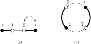
Figure 4: Graphic explanation of the notion “loop-like substring”. (a) The substring $(2{\bar{3}})({\bar{2}}3)$ can be transformed into the form of an adjacent substring (in the sense of Definition 5.7) by flipping arguments in the second kernel, $({\bar{2}}3)\mapsto(3{\bar{2}})$. (b) The emerging adjacent substring $(2{\bar{3}})(3{\bar{2}})$ can clearly be depicted in the form of a loop by gluing the arguments $2$ and $\bar{2}$ together.

5.2.3 Counting longest loop-like substrings ${\cal S}_{i}^{(\ell)}$ of the length $\ell$

Although in this subsection, we are going to concentrate on the longest loop-like substrings of the length $\ell$, our main counting result given by Lemma 5.3 stays valid for loop-like substrings of a smaller length $1\leq p<\ell$.

Lemma 5.3. The ordered Pfaffian expansion contains $(2\ell)!!\,(2\ell-2)!!$ longest loop-like strings of the length $\ell$.

Proof. Let ${\cal N}_{L}(\ell)$ be the total number of loop-like strings of the length $\ell$ in the ordered Pfaffian expansion and let $n_{L}(\ell)$ denote the number of equivalence classes all longest loop-like strings can be assigned to. Following Lemma 5.1, the two are related to each other as

$${\cal N}_{L}(\ell)=(2\ell)!!\,n_{L}(\ell),$$ (1.1cghaw)

because each equivalence class ${\cal C}_{j}$ contains precisely $(2\ell)!!$ equivalent strings (see Definition 5.3). It thus remains to determine $n_{L}(\ell)$ that can equally be interpreted as a number of inequivalent longest loop-like strings of the length $\ell$.

The latter can be evaluated by counting the number of ways, $n_{L}(\ell+1)$, all inequivalent longest loop-like strings of the length $\ell+1$ can be generated from those longest of the length $\ell$. Since both numbers, $n_{L}(\ell)$ and $n_{L}(\ell+1)$, refer to the longest loop-like strings, the two correspond to the Pfaffians of matrices of the size $\ell\times\ell$ and $(\ell+1)\times(\ell+1)$, correspondingly. In the language of strings, an increase of the matrix size by one leads to the appearance of an additional pair of arguments $(z_{\ell+1},{\bar{z}}_{\ell+1})$ in a string of the length $\ell+1$.

We claim that

$$n_{L}(\ell+1)=2\ell\,n_{L}(\ell).$$ (1.1cghax)

To prove this, we concentrate on a given longest loop-like string of the length $\ell$ and add to it an additional pair of arguments $(z_{\ell+1},{\bar{z}}_{\ell+1})$:

$$(z_{\ell+1},{\bar{z}}_{\ell+1})\;\;\;\otimes\underbrace{\prod_{k=1}^{\ell}(w_{\sigma_{i}(2j_{k}+1)},w_{\sigma_{i}(2j_{k}+2)})}_{{\rm longest\;loop-like\;string\;of\;the\;length\;}\ell}.$$ (1.1cghay)

Here, $\sigma_{i}$ is a particular permutation of $2\ell$ arguments (1.1cghz) corresponding to a longest loop-like string of the length $\ell$. The resulting string (1.1cghay) is not a longest loop-like string of the length $\ell+1$ (rather, it is composed of two loop-like strings of the lengths $1$ and $\ell$, respectively). Since a loop-like string necessarily assumes the presence of a fragment $(z_{\ell+1},\cdots)\,(\cdots,{\bar{z}}_{\ell+1})$ somewhere in the string, one has to exchange either $z_{\ell+1}$ or ${\bar{z}}_{\ell+1}$ with one of the arguments belonging to the original longest loop-like string of the length $\ell$. Clearly, there exist $2\ell$ exchange options for each argument, $z_{\ell+1}$ (or ${\bar{z}}_{\ell+1}$). As a result, we arrive at the relation (1.1cghax). Given $n_{L}(1)=1$, we derive the desired result by induction:

$$n_{L}(\ell)=(2\ell-2)!!$$ (1.1cghaz)

Combining it with (1.1cghaw) completes the proof. $\;\;\;\blacksquare$

5.2.4 Adjacent vs non-adjacent loop-like substrings

Further classification of loop-like substrings is needed in order to prepare ourselves to the proof of the Pfaffian integration theorem.

Definition 5.7. A loop-like substring ${\cal S}_{i}^{(p)}$ of the length $p=\|{\cal S}_{i}^{(p)}\|$ is called adjacent loop-like substring,  or simply a loop, if it is represented by a product

$${\cal S}_{i}^{(p)}=\prod_{k=1}^{p}Q_{n}(w_{\sigma_{i}(2j_{k}+1)},w_{\sigma_{i}(2j_{k}+2)})$$

of $p$ kernels such that:

1. The first argument of the first kernel and the second argument of the last, $p$-th kernel, are complex conjugate of each other,

   $$w_{\sigma_{i}(2j_{1}+1)}={\bar{w}}_{\sigma_{i}(2j_{p}+2)}.$$

2. For each pair of neighbouring kernels in the string, the second argument of the left kernel in the pair and the first argument of the right kernel in the pair are complex conjugate of each other,

   $$w_{\sigma_{i}(2j_{k}+2)}={\bar{w}}_{\sigma_{i}(2j_{k+1}+1)},\;\;\;\;k=1,\cdots,p-1.$$

   
   

Example 5.7. Out of $16$ longest loop-like strings arising in the Pfaffian expansion for $\ell=2$ , the following eight are adjacent:

$$-(1{\bar{2}})(2{\bar{1}}),\;\;-({\bar{2}}1)({\bar{1}}2),\;\;-({\bar{1}}2)({\bar{2}}1),\;\;-(2{\bar{1}})(1{\bar{2}}),$$

$$+(12)({\bar{2}}{\bar{1}}),\;\;+(21)({\bar{1}}{\bar{2}}),\;\;+({\bar{1}}{\bar{2}})(21),\;\;+({\bar{2}}{\bar{1}})(12).$$

Notice that although longest loop-like strings have been considered in the above example, the notion of an adjacent string is equally relevant for a loop-like string of smaller length.

Lemma 5.4. Out of $(2\ell)!!(2\ell-2)!!$ longest loop-like strings of the length $\ell$ associated with an ordered Pfaffian expansion, exactly $(2\ell)!!$ are adjacent.

Proof. To count the total number ${\cal N}_{A}(\ell)$ of all adjacent loop-like strings of the length $\ell$, we consider a specific pair of adjacent loop-like strings of the length $\ell$ represented by the sequences of arguments

$$(z_{j_{1}},\underbrace{{\bar{z}}_{j_{2}})(z_{j_{2}}}_{{\rm pair\;\natural\;1}},\underbrace{{\bar{z}}_{j_{3}})(z_{j_{3}}}_{{\rm pair\;\natural\;2}},{\bar{z}}_{j_{4}})\cdots(z_{j_{p-1}},{\bar{z}}_{j_{p}})\cdots(z_{j_{\ell-1}},\underbrace{{\bar{z}}_{j_{\ell}})(z_{j_{\ell}}}_{{\rm pair\;\natural\;(\ell-1)}},{\bar{z}}_{j_{1}})$$

and

$$({\bar{z}}_{j_{1}},\underbrace{{\bar{z}}_{j_{2}})(z_{j_{2}}}_{{\rm pair\;\natural\;1}},\underbrace{{\bar{z}}_{j_{3}})(z_{j_{3}}}_{{\rm pair\;\natural\;2}},{\bar{z}}_{j_{4}})\cdots(z_{j_{p-1}},{\bar{z}}_{j_{p}})\cdots(z_{j_{\ell-1}},\underbrace{{\bar{z}}_{j_{\ell}})(z_{j_{\ell}}}_{{\rm pair\;\natural\;(\ell-1)}},z_{j_{1}}).$$

Here, the mutually distinct $j_{p}$ take the values from $1$ to $\ell$. The two strings are identical up to an exchange of the first and the last arguments $z_{j_{1}}\rightleftarrows{\bar{z}}_{j_{1}}$. The remaining $2(\ell-1)$ arguments are distributed between the kernels in such a way that an adjacent string is formed in accordance with the Definition 5.7; the $(\ell-1)$ underbraces identifying $(\ell-1)$ pairs of complex conjugate arguments highlight the structure of an adjacent string.

The total number ${\cal N}_{A}(\ell)$ of all adjacent loop-like strings of the length $\ell$ equals the number of ways to generate those strings from the two depicted above. As soon as there are (i) $\ell$ ways to assign a number from $1$ to $\ell$ to the label $j_{1}$, (ii) $(\ell-1)!$ ways to assign the remaining $(\ell-1)$ numbers to the $(\ell-1)$ pairs left (labelled by $j_{2},\cdots,j_{\ell}$), and (iii) $2^{\ell-1}$ ways to exchange the arguments $z_{j_{k}}\rightleftarrows{\bar{z}}_{j_{k}}$ ($k=2,\cdots,\ell$) within those $(\ell-1)$ pairs, we derive:

$${\cal N}_{A}(\ell)=2\times\ell\times(\ell-1)!\times 2^{\ell-1}=(2\ell)!!$$ (1.1cghba)

End of proof. $\;\;\;\blacksquare$

Remark 5.1. Since the above reasoning holds for loop-like (sub)strings of any length $1\leq p\leq\ell$, one concludes that the total number of adjacent (sub)strings of the length $p$ equals ${\cal N}_{A}(p)=(2p)!!$.

Lemma 5.5. Any loop-like (sub)string of the length $p$ can be transformed into an adjacent (sub)string of the same length by means of proper (i) permutation of kernels and/or (ii) permutation of intra-kernel arguments.

Proof. To be coherent with the notations used in the proof of the Lemma 5.3, we deal below with a loop-like string of the length $\ell$. However, the very same argument applies to any loop-like (sub)string of the length $1\leq p\leq\ell$ so that our proof (based on mathematical induction) holds generally.

(i) For $\ell=1$ and $\ell=2$, the Lemma’s statement is obviously true. Indeed, a loop-like string of the length $\ell=1$ is automatically an adjacent one. For $\ell=2$, a loop-like string composed of two kernels is reduced to an adjacent string by utmost one intra-kernel permutation of arguments.

(ii) Now we assume the Lemma to hold for loop-like (sub)strings of the length $\ell$ (that is, that any loop-like string of the length $\ell$ can be reduced to an adjacent string by means of the two types of allowed operations).

(iii) Given the previous assumption, we have to show that a loop-like (sub)string of the length $(\ell+1)$ can also be reduced to an adjacent (sub)string. It follows from the proof of the Lemma 5.3 (see the discussion around (1.1cghay)) that a loop-like string of the length $(\ell+1)$ can be generated from a loop-like string of a smaller length $\ell$ by adding an additional pair of arguments $(z_{\ell+1},{\bar{z}}_{\ell+1})$ followed by exchange of either $z_{\ell+1}$ or ${\bar{z}}_{\ell+1}$ with one of the arguments of the original loop-like string of the length $\ell$. Since, under the induction assumption (ii), the latter can be made adjacent,

$$(z_{\ell+1},{\bar{z}}_{\ell+1})\,\otimes\,\underbrace{[(z_{j_{1}},\dots)\,\cdots\,(\dots,{\bar{z}}_{j_{q}})\,(z_{j_{q}},\dots)\,\cdots\,(\dots,{\bar{z}}_{j_{1}})]}_{{\rm adjacent\;string\;of\;the\;length\;}\ell},$$ (1.1cghbb)

one readily concludes that we are only two steps away from forming an adjacent string of the length $(\ell+1)$ out of (1.1cghbb). Indeed, an exchange of arguments ${\bar{z}}_{\ell+1}\rightleftarrows{\bar{z}}_{j_{q}}$ brings (1.1cghbb) to the form

$$(z_{\ell+1},{\bar{z}}_{j_{q}})\,(z_{j_{1}},\dots)\,\cdots\,(\dots,{\bar{z}}_{\ell+1})\,(z_{j_{q}},\dots)\,\cdots\,(\dots,{\bar{z}}_{j_{1}})$$ (1.1cghbc)

which boils down to the required adjacent string

$$\underbrace{(z_{j_{1}},\dots)\,\cdots\,(\dots,{\bar{z}}_{\ell+1})\,(z_{\ell+1},{\bar{z}}_{j_{q}})\,(z_{j_{q}},\dots)\,\cdots\,(\dots,{\bar{z}}_{j_{1}})}_{{\rm adjacent\;string\;of\;the\;length\;}(\ell+1)}$$ (1.1cghbd)

upon moving the pair $(z_{\ell+1},{\bar{z}}_{j_{q}})$ through $(q-1)$ pairs on the right. Exchanging ${\bar{z}}_{\ell+1}\rightleftarrows{z}_{j_{q}}$ instead can be done in the same way. $\;\;\;\blacksquare$

Remark 5.2. The reduction of a loop-like (sub)string to an adjacent (sub)string is not unique. For instance, the loop-like string

$$+(1{\bar{3}})({\bar{2}}3)({\bar{1}}2)$$

(see the first term in (1.1cghad)) can be reduced, by permutation of kernels and permutation of intra-kernel arguments, to one of the following adjacent strings:

$$+(1{\bar{3}})(3{\bar{2}})(2{\bar{1}}),\;\;-({\bar{1}}2)({\bar{2}}3)({\bar{3}}1),$$

$$+(2{\bar{1}})(1{\bar{3}})(3{\bar{2}}),\;\;-({\bar{2}}3)({\bar{3}}1)({\bar{1}}2),$$

$$+(3{\bar{2}})(2{\bar{1}})(1{\bar{3}}),\;\;-({\bar{3}}1)({\bar{1}}2)({\bar{2}}3).$$ (1.1cghbe)

To handle the problem of the non-unique reduction of a loop-like string to an adjacent string, the notion of string handedness has to be introduced.

5.2.5 Handedness of an adjacent substring

Definition 5.8. Close an adjacent substring ${\cal S}$ into a loop by “gluing” the right argument of the last kernel with the left argument of the first kernel below the chain as in Figure 4.,

$${\cal S}:\;\;\rightsquigarrow\bullet\underbrace{(w_{j_{1}},{\bar{w}}_{j_{2}})}_{{\rm first\;kernel}}\cdot\,(w_{j_{2}},{\bar{w}}_{j_{3}})\cdots(w_{j_{q-1}},{\bar{w}}_{j_{q}})\cdots(w_{j_{p-1}},{\bar{w}}_{j_{p}})\cdot\underbrace{(w_{j_{p}},{\bar{w}}_{j_{1}})}_{{\rm last\;kernel}}\bullet\rightsquigarrow$$

(here, a set of the arguments $(w_{1},\cdots,w_{2p})$ is specified by (1.1cghz) with $\ell$ set to $p$, and the symbol $\bullet$ denotes a gluing point). Read the arguments of a loop, one after the other, in a clockwise direction (as depicted by the symbol $\rightsquigarrow$), starting with ${\bar{w}}_{j_{1}}$ until you arrive at $w_{j_{p}}$. If $\alpha_{R}$ is the number of times an argument $z_{j_{q}}$ is followed by its conjugate ${\bar{z}}_{j_{q}}$ for all $q\in(1,\cdots,p)$,

$$(\dots,z_{j_{q}})\cdot({\bar{z}}_{j_{q}},\dots),$$

an adjacent substring ${\cal S}$ is said to have the handedness ${\mathbb{H}}(\alpha_{L},\alpha_{R})$, where $\alpha_{L}=p-\alpha_{R}$.

Example 5.8. The handedness of eight adjacent strings considered in the Example 5.7 with $p=l=2$ is listed below:

$${\mathbb{H}}(2,0),\;\;{\mathbb{H}}(0,2),\;\;{\mathbb{H}}(0,2),\;\;{\mathbb{H}}(2,0),$$

$${\mathbb{H}}(1,1),\;\;{\mathbb{H}}(1,1),\;\;{\mathbb{H}}(1,1),\;\;{\mathbb{H}}(1,1).$$ (1.1cghbf)

Lemma 5.6. Out of $(2\ell)!!$ adjacent strings of the length $\ell$ arising in an ordered Pfaffian expansion, there are exactly

$${\cal N}_{\alpha}(\ell)=\ell!\,{\ell\choose\alpha}$$ (1.1cghbg)

strings with the handedness ${\mathbb{H}}(\alpha,\ell-\alpha)$.

Proof. A string with the handedness ${\mathbb{H}}(\alpha,\ell-\alpha)$ closed into a loop (see Definition 5.8) contains $\alpha$ “left” fragments $(\dots,{\bar{z}}_{j_{q}})\cdot(z_{j_{q}},\dots)$ and $(\ell-\alpha)$ “right” fragments $(\dots,z_{j_{q}})\cdot({\bar{z}}_{j_{q}},\dots)$ with the opposite order of complex conjugation in the nearest neighbouring kernels; each fragment is labelled by an integer number $j_{q}\in(1,\cdots,\ell)$. To count a total number of all strings with the handedness ${\mathbb{H}}(\alpha,\ell-\alpha)$, we notice that there exist ${\ell\choose\alpha}$ ways to distribute “left” and “right” fragments on the loop, and $\ell!$ ways to assign $\ell$ integer numbers (from $1$ to $\ell$) to the labels $j_{1},\cdots,j_{\ell}$. Applying the combinatorial multiplication rule completes the proof. $\;\;\;\blacksquare$

Remark 5.3. It is instructive to realise that the Lemma 5.4 can be seen as a corollary to the Lemma 5.6. Indeed, the total number of all adjacent strings of the length $\ell$ is nothing but

$$\sum_{\alpha=0}^{\ell}{\cal N}_{\alpha}(\ell)=\ell!\,\sum_{\alpha=0}^{\ell}{\ell\choose\alpha}=(2\ell)!!$$

Not unexpectedly, this result is in concert with the Lemma 5.4.

Corollary 5.2. The number of adjacent substrings of the length $p$, $1\leq p<\ell$, with the handedness $\mathbb{H}(\alpha,p-\alpha)$ equals

$${\cal N}_{\alpha}(p)=p!\,{p\choose\alpha}.$$ (1.1cghbh)

The total number of all adjacent substrings of the length $p$ is $(2p)!!$

Proof. Follow the proof of the Lemma 5.6 and the Remark 5.3 with $\ell$ replaced by $p$. $\;\;\;\blacksquare$

Example 5.9. Out of $16$ longest loop-like strings arising in the Pfaffian expansion for $\ell=2$, there are eight adjacent as explicitly specified in Example 5.7. The handedness of those strings was considered in Example 5.8. In accordance with the Lemma 5.6, there must exist ${\cal N}_{0}(2)=2$ strings of the handedness ${\mathbb{H}}(0,2)$, ${\cal N}_{2}(2)=2$ strings of the handedness ${\mathbb{H}}(2,0)$, and ${\cal N}_{1}(2)=4$ strings of the handedness ${\mathbb{H}}(1,1)$. Direct counting (5.2.5) confirms that this is indeed the case.

5.2.6 Equivalence classes of adjacent (sub)strings

Having defined a notion of the handedness of an adjacent string, we are back to the issue of a non-uniqueness of reduction of a loop-like string to an adjacent one. To deal with the indicated non-uniqueness problem, we would like to define, and explicitly identify, all distinct equivalence classes for $(2\ell)!!$ adjacent strings arising in the context of an ordered Pfaffian expansion.

Definition 5.9. Two adjacent strings, ${\cal S}_{i}$ and ${\cal S}_{j}$, are said to be equivalent adjacent strings, ${\cal S}_{i}\sim{\cal S}_{j}$, if they can be obtained from each other by (i) permutation of kernels and/or (ii) intra-kernel permutation of arguments.

Example 5.10. The six adjacent strings (5.2.4) are equivalent to each other.

Definition 5.10. A group of equivalent adjacent strings is called the equivalence class of adjacent strings. The $j$-th equivalence class to be denoted ${\cal AC}_{j}$ consists of $\|{\cal AC}_{j}\|$ equivalent adjacent strings.

Lemma 5.7. All $(2\ell)!!$ adjacent strings arising in the ordered Pfaffian expansion can be assigned to $(2\ell-2)!!$ equivalence classes $\{{\cal AC}_{1},\cdots,{\cal AC}_{(2\ell-2)!!}\}$ of adjacent strings, each class containing $2\ell$ equivalent adjacent strings: $\|{\cal AC}_{j}\|=2\ell$ for all $j\in 1,\cdots,(2\ell-2)!!$.

Proof. Let us concentrate on a given adjacent string ${\cal S}$ with the handedness ${\mathbb{H}}(\alpha,\ell-\alpha)$ that belongs to an equivalence class ${\cal AC}_{j}$ and count a number of ways to generate equivalent strings out of it by means of (i) permutation of kernels and/or (ii) intra-kernel permutation of arguments without destroying the adjacency property. Two complementary generating mechanisms exist.

• First way (M1): One starts with an adjacent string of the handedness ${\mathbb{H}}(\alpha,\ell-\alpha)$,

  $$\rightsquigarrow\bullet\underbrace{(w_{j_{1}},{\bar{w}}_{j_{2}})}_{{\rm first\;kernel}}\cdot\,(w_{j_{2}},{\bar{w}}_{j_{3}})\cdots(w_{j_{p-1}},{\bar{w}}_{j_{p}})\cdots(w_{j_{\ell-1}},{\bar{w}}_{j_{\ell}})\cdot\underbrace{(w_{j_{\ell}},{\bar{w}}_{j_{1}})}_{{\rm last\;kernel}}\bullet\rightsquigarrow$$ (1.1cghbi)

  (the reader is referred to the Definition 5.8 for the notation used), simultaneously flips the intra-kernel arguments in all $\ell$ kernels,

  $$\;\;\;\;\;\;\;\underbrace{({\bar{w}}_{j_{2}},w_{j_{1}})}_{{\rm first\;kernel}}\cdot\,({\bar{w}}_{j_{3}},w_{j_{2}})\cdots({\bar{w}}_{j_{p}},w_{j_{p-1}})\cdots({\bar{w}}_{j_{\ell}},w_{j_{\ell-1}})\cdot\underbrace{({\bar{w}}_{j_{1}},w_{j_{\ell}})}_{{\rm last\;kernel}}\ ,$$

  and further permutes the kernels in a fan-like way so that the last $\ell$-th kernel in the string becomes the first, the $(\ell-1)$-th kernel in the string becomes the second, etc.:

  $$\rightsquigarrow\bullet\underbrace{({\bar{w}}_{j_{1}},w_{j_{\ell}})}_{{\rm last\;kernel}}\cdot\,({\bar{w}}_{j_{\ell}},w_{j_{\ell-1}})\cdots({\bar{w}}_{j_{p}},w_{j_{p-1}})\cdots({\bar{w}}_{j_{3}},w_{j_{2}})\cdot\underbrace{({\bar{w}}_{j_{2}},w_{j_{1}})}_{{\rm first\;kernel}}\bullet\rightsquigarrow$$ (1.1cghbj)

  The so obtained adjacent string is equivalent to the initial one (1.1cghbi) but possesses the complementary handedness ${\mathbb{H}}(\ell-\alpha,\alpha)$.
  

• Second way (M2): One starts with an adjacent string of the handedness ${\mathbb{H}}(\alpha,\ell-\alpha)$, and permutes the $\ell$ kernels in a cyclic manner to generate $(\ell-1)$ additional (but equivalent) adjacent strings with the same handedness (to visualise the process, one may think of moving a gluing point $\bullet$ through the kernels in (1.1cghbi)).

The two mechanisms, M1 and M2, combined together bring up $2\ell$ equivalent adjacent strings due to the combinatorial multiplication rule. As a result, we conclude that $\|{\cal AC}_{j}\|=2\ell$. Consequently, the number of distinct equivalence classes equals $(2\ell)!!/(2\ell)=(2\ell-2)!!$. $\;\;\;\blacksquare$

Example 5.11. To illustrate the Lemma 5.7, we consider an ordered Pfaffian expansion for $\ell=2$ as detailed in the Example 5.1. The eight adjacent strings of the length $\ell=2$ were specified in the Example 5.7; their handedness was considered in the Example 5.8. In accordance with the Lemma 5.7, there should exist $2$ distinct equivalence classes, each containing $4$ adjacent strings. Indeed, one readily verifies that those two equivalence classes are

$${\cal AC}_{1}:\;\;-(1{\bar{2}})(2{\bar{1}}),\;\;-({\bar{2}}1)({\bar{1}}2),\;\;-({\bar{1}}2)({\bar{2}}1),\;\;-(2{\bar{1}})(1{\bar{2}})$$

and

$${\cal AC}_{2}:\;\;+(12)({\bar{2}}{\bar{1}}),\;\;+(21)({\bar{1}}{\bar{2}}),\;\;+({\bar{1}}{\bar{2}})(21),\;\;+({\bar{2}}{\bar{1}})(12).$$

$\begin{array}[]{lll}{\begin{minipage}{390.25755pt} \raisebox{-14.22636pt}{\shadowbox{ \begin{minipage}{130.08621pt} \begin{center} \small{ {\bf Longest Loop-Like Strings} \newline {Total amount: $(2\ell)!!(2\ell-2)!!$}} \end{center} \end{minipage}}} = \raisebox{-14.22636pt}{\shadowbox{ \begin{minipage}{101.17755pt} \begin{center} \small{ {\bf~{}Adjacent Strings} \newline {Total amount: $(2\ell)!!$}} \end{center} \end{minipage}}} $\bigcup$ \raisebox{-14.22636pt}{\shadowbox{ \begin{minipage}{79.49744pt} \begin{center} \small{ {\bf Non-Adjacent}} \newline \small{{\bf Strings}} \end{center} \end{minipage}}} \end{minipage}}&{}&{}\\ {}&{}&{}\\ {}&{}&{}\end{array}\newline \qquad\left\{\begin{array}[]{l}{\cal C}_{1}\\ \cdots\\ {\cal C}_{j}\\ \cdots\\ {\cal C}_{(2\ell-2)!!}\end{array}\right\}\ \rightsquigarrow\;\left\{\begin{array}[]{ll}{\cal AC}_{1}&\rightsquigarrow\begin{array}[]{l}\raisebox{-14.22636pt}{\shadowbox{ \begin{minipage}{101.17755pt} \begin{center} \small{ $\ell$ strings: ${\mathbb{H}}(\alpha_{1},\ell-\alpha_{1})$\\ $\ell$ strings: ${\mathbb{H}}(\ell-\alpha_{1},\alpha_{1})$} \end{center} \end{minipage}}}\end{array}\\ \cdots\\ {\cal AC}_{j}&\rightsquigarrow\begin{array}[]{l}\raisebox{-14.22636pt}{\shadowbox{ \begin{minipage}{101.17755pt} \begin{center} \small{ $\ell$ strings: ${\mathbb{H}}(\alpha_{j},\ell-\alpha_{j})$\\ $\ell$ strings: ${\mathbb{H}}(\ell-\alpha_{j},\alpha_{j})$} \end{center} \end{minipage}}}\end{array}\\ \cdots\\ {\cal AC}_{(2\ell-2)!!}&\rightsquigarrow\begin{array}[]{l}\raisebox{-14.22636pt}{\shadowbox{ \begin{minipage}{144.54pt} \begin{center} \small{ $\ell$ strings: ${\mathbb{H}}(\alpha_{(2\ell-2)!!},\ell-\alpha_{(2\ell-2)!!})$\\ $\ell$ strings: ${\mathbb{H}}(\ell-\alpha_{(2\ell-2)!!},\alpha_{(2\ell-2)!!})$} \end{center} \end{minipage}}}\end{array}\end{array}\right\}\newline \newline \newline$

Figure 5: Any longest loop-like string from the equivalence classes $\{{\cal C}_{1},\cdots,{\cal C}_{(2\ell-2)!!}\}$ can be reduced to an adjacent string belonging to one of the equivalence classes $\{{\cal AC}_{1},\cdots,{\cal AC}_{(2\ell-2)!!}\}$ of adjacent strings by means of proper permutation of kernels and/or permutation of intra-kernel arguments (Lemma 5.5). This reduction is non-unique (Remark 5.2). Each equivalence class ${\cal AC}_{j}$ of adjacent strings contains $\ell$ adjacent strings of the handedness ${\mathbb{H}}(\alpha_{j},\ell-\alpha_{j})$ and $\ell$ adjacent strings of the complementary handedness ${\mathbb{H}}(\ell-\alpha_{j},\alpha_{j})$ (Remark 5.4). Notice that two distinct equivalence classes ${\cal AC}_{i}$ and ${\cal AC}_{j}$ (where $i\neq j$) may have the same values for $\alpha$: $\alpha_{i}=\alpha_{j}$.

Remark 5.4. In fact, a generic prescription can be given to build $(2\ell-2)!!$ distinct equivalence classes $\{{\cal AC}_{1},\cdots,{\cal AC}_{(2\ell-2)!!}\}$ for $(2\ell)!!$ adjacent strings arising in the ordered Pfaffian expansion. Because of the “duality” between equivalent adjacent strings with complementary handedness ${\mathbb{H}}(\alpha,\ell-\alpha)$ and ${\mathbb{H}}(\ell-\alpha,\alpha)$ discussed in the proof of the Lemma 5.6, the adjacent strings whose handedness ${\mathbb{H}}(\alpha,\ell-\alpha)$ is restricted by the inequality $0\leq\alpha\leq\lfloor\ell/2\rfloor$ will form a natural basis in the consideration to follow.

• The case $\ell=2\lambda+1$ odd.
  
  (i) For $0\leq\alpha_{1}\leq\lambda$, (i.a) pick up an adjacent string with the handedness ${\mathbb{H}}(\alpha_{1},\ell-\alpha_{1})$, out of ${\cal N}_{\alpha_{1}}(\ell)$, and generate $\ell$ equivalent adjacent strings with the same handedness through the mechanism M2 of the Lemma 5.7. (i.b) Apply the mechanism M1 of the same Lemma to each of the $\ell$ adjacent strings generated in (i.a) to create $\ell$ more equivalent adjacent strings of the handedness ${\mathbb{H}}(\ell-\alpha_{1},\alpha_{1})$ hereby raising their total amount to $2\ell$. The strings generated in (i.a) and (i.b) are said to belong to the equivalence class ${\cal AC}_{1}$.
  
  (ii) To generate the next equivalence class ${\cal AC}_{2}\neq{\cal AC}_{1}$, pick up an adjacent string not belonging to ${\cal AC}_{1}$ with the handedness ${\mathbb{H}}(\alpha_{2},\ell-\alpha_{2})$ out of $({\cal N}_{\alpha_{1}}(\ell)-\ell)$ left (again, $\alpha_{2}$ is restricted to $0\leq\alpha_{2}\leq\lambda$), and repeat the actions described in (i.a) and (i.b) to generate another set of $2\ell$ equivalent strings. These will belong to the equivalence class ${\cal AC}_{2}$ which is distinct from ${\cal AC}_{1}$.
  
  (iii) To generate the $j$-th equivalence class ${\cal AC}_{j}$, one picks up an adjacent string out of $({\cal N}_{\alpha_{1}}(\ell)-(j-1)\ell)$ left and repeats the actions sketched in (ii).
  
  (iv) The procedure stops once there are no adjacent strings left. Obviously, the total number of equivalence classes is

  $$\frac{1}{\ell}\sum_{\alpha=0}^{\lfloor\ell/2\rfloor}{\cal N}_{\alpha}(\ell)=(2\lambda)!\sum_{\alpha=0}^{\lambda}{2\lambda+1\choose\alpha}=(2\lambda)!\,2^{2\lambda}=(2\ell-2)!!$$ (1.1cghbk)

  This is in concert with the Lemma 5.7.
  

• The case $\ell=2\lambda$ even.
  
  In this case, special care should be exercised for the set of adjacent strings with the handedness ${\mathbb{H}}(\lambda,\lambda)$ because these adjacent strings are self-complementary: the mechanism M1 applied to any of those adjacent strings generates a string with the same, not complementary, handedness. The latter circumstance can readily be accommodated when giving a prescription for building $(2\ell-2)!!$ distinct equivalence classes of adjacent strings.
  
  (i) First, we separate all adjacent strings with the handedness ${\mathbb{H}}(\alpha,\ell-\alpha)$ where $0\leq\alpha\leq\lambda-1$ and apply a procedure identically equivalent to that described for the case $\ell$ odd to generate distinct equivalence classes of adjacent strings. The total amount of distinct equivalence classes built in this way equals

  $$L_{1}=\frac{1}{\ell}\sum_{\alpha=0}^{\lfloor\ell/2\rfloor-1}{\cal N}_{\alpha}(\ell)=(2\lambda-1)!\sum_{\alpha=0}^{\lambda-1}{2\lambda\choose\alpha}=(2\ell-2)!!-\frac{(2\lambda-1)!}{2}\,{2\lambda\choose\lambda}.$$ (1.1cghbl)

  
  
  

  (ii) Second, having generated in the previous step $L_{1}$ distinct equivalence classes $\{{\cal AC}_{1},\cdots,{\cal AC}_{L_{1}}\}$ of adjacent strings, we concentrate on the adjacent strings with the handedness ${\mathbb{H}}(\lambda,\lambda)$ not treated so far. To this end, we (ii.a) pick up an adjacent string out of ${\cal N}_{\lambda}(2\lambda)$ with the handedness ${\mathbb{H}}(\lambda,\lambda)$ and perform the operations M1 and M2 to generate $2\ell=4\lambda$ equivalent strings with the same handedness. The $2\ell$ equivalent adjacent strings will belong to a certain equivalence class, say, ${\cal AC}_{L_{1}+1}$. (ii.b) In the next step, we pick up an adjacent string with the handedness ${\mathbb{H}}(\lambda,\lambda)$ out of $({\cal N}_{\lambda}(2\lambda)-2\ell)$ left, and perform the operations detailed in (ii.a) in order to generate yet another set of $2\ell$ equivalent adjacent strings belonging to an equivalence class ${\cal AC}_{L_{1}+2}$. (ii.c) We proceed further on until the last available equivalence class composed of $2\ell$ adjacent strings is formed, ${\cal AC}_{L_{1}+L_{2}}$, where $L_{2}$ equals

  $$L_{2}=\frac{1}{2\ell}\,{\cal N}_{\lambda}(\ell)=\frac{(2\lambda-1)!}{2}\,{2\lambda\choose\lambda}.$$ (1.1cghbm)

  Hence, for $\ell=2\lambda$, the total number of equivalence classes for adjacent strings equals

  $$L_{1}+L_{2}=(2\ell-2)!!$$ (1.1cghbn)

  as expected from the Lemma 5.7.

5.3 Integrating out all longest loop-like strings of the length $\ell$

More spadework is needed to prove the Pfaffian integration theorem. Below, we will be interested in calculating the contribution $C_{L}(\ell)$ of longest loop-like strings (of the length $\ell$) into the sought integral (1.1cghbd):

$$C_{L}(\ell) =\int_{{\mathbb{C}}}\,\prod_{j=1}^{\ell}\,d\pi(z_{j})\,\,\left({\rm pf\,}\left[\begin{array}[]{cc}Q_{n}(z_{i},z_{j})&Q_{n}(z_{i},{\bar{z}}_{j})\\ Q_{n}({\bar{z}}_{i},z_{j})&Q_{n}({\bar{z}}_{i},{\bar{z}}_{j})\\ \end{array}\right]_{2\ell\times 2\ell}\right)_{{\scriptsize\begin{array}[]{c}{\rm longest}\\ {\rm loop-like\;strings}\end{array}}}$$ (1.1cghbs)

$$=\frac{1}{2^{\ell}\ell!}\int_{{\mathbb{C}}}\,\prod_{j=1}^{\ell}\,d\pi(z_{j})\,\,\sum_{\sigma\in S^{\prime}_{2\ell}}{\rm sgn}(\sigma)\,\prod_{j=0}^{\ell-1}Q_{n}(w_{\sigma(2j+1)},w_{\sigma(2j+2)}).$$ (1.1cghbt)

In the second line of (1.1cghbs), only that part of the ordered Pfaffian expansion (1.1cghx) appears which corresponds to a set of all loop-like strings of the length $\ell$. They are accounted for by picking up proper permutations $S^{\prime}_{2\ell}\subset S_{2\ell}$ in the expansion (1.1cghx),

$$S^{\prime}_{2\ell}\;\mapsto\;({\rm longest\;loop-like\;strings\;of\;the\;length\;\ell}).$$

Although, in accordance with the Lemma 5.3, the number of terms in the expansion (1.1cghbs) equals ${\cal N}_{L}(\ell)=(2\ell)!!(2\ell-2)!!$, there is no need to integrate all of them out because various loop-like strings belonging to the same equivalence class yield identical contributions. The latter observation effectively reduces the number of terms in (1.1cghbs) so that

$$C_{L}(\ell)=\frac{(2\ell)!!}{2^{\ell}\ell!}\int_{{\mathbb{C}}}\,\prod_{j=1}^{\ell}\,d\pi(z_{j})\,\,\sum_{\sigma\in S^{\prime\prime}_{2\ell}}{\rm sgn}(\sigma)\,\prod_{j=0}^{\ell-1}Q_{n}(w_{\sigma(2j+1)},w_{\sigma(2j+2)}).$$ (1.1cghbu)

Here, the prefactor $(2\ell)!!=2^{\ell}\ell!$ equals the number of longest loop-like strings in each equivalence class; the $\sigma$-series runs over the permutations $S^{\prime\prime}_{2\ell}\subset S^{\prime}_{2\ell}$ corresponding to $n_{L}(\ell)=(2\ell-2)!!$ longest loop-like strings, each of them being a representative of one distinct equivalence class,

$$S^{\prime\prime}_{2\ell}\;\mapsto\;\{{\cal S}_{1}\in{\cal C}_{1},\cdots,{\cal S}_{(2\ell-2)!!}\in{\cal C}_{(2\ell-2)!!}\},$$ (1.1cghbv)

see the Lemma 5.3. There are $(2\ell-2)!!$ terms in (1.1cghbu).

To perform the integration explicitly, one has to reduce the longest loop-like strings in (1.1cghbu) to the form of adjacent strings as discussed in the Lemma 5.5. In accordance with the Lemma 5.7, there exist $(2\ell-2)!!$ equivalence classes $\{{\cal AC}_{1},\cdots,{\cal AC}_{(2\ell-2)!!}\}$ of adjacent strings, each of them containing $2\ell$ equivalent adjacent strings (see also Fig. 5). This results in the representation

$$C_{L}(\ell)=\int_{{\mathbb{C}}}\,\prod_{j=1}^{\ell}\,d\pi(z_{j})\,\,\sum_{\sigma\in{\tilde{S}}^{\prime\prime}_{2\ell}}{\rm sgn}(\sigma)\,\prod_{j=0}^{\ell-1}Q_{n}(w_{\sigma(2j+1)},w_{\sigma(2j+2)}),$$ (1.1cghbw)

where the $\sigma$-series runs over the permutations ${\tilde{S}}^{\prime\prime}_{2\ell}\subset S^{\prime}_{2\ell}$ corresponding to $(2\ell-2)!!$ adjacent loop-like strings of the length $\ell$, each of them being a representative of each one of existing equivalence classes of adjacent strings,

$${\tilde{S}}^{\prime\prime}_{2\ell}\;\mapsto\;\{\tilde{{\cal S}}_{1}\in{\cal AC}_{1},\cdots,{\tilde{\cal S}}_{(2\ell-2)!!}\in{\cal AC}_{(2\ell-2)!!}\}.$$ (1.1cghbx)

The number of terms in (1.1cghbw) is $(2\ell-2)!!$.

To proceed, we rewrite (1.1cghbw) in a more symmetric form that treats all adjacent strings on the same footing:

$$C_{L}(\ell)=\frac{1}{2\ell}\,\int_{{\mathbb{C}}}\,\prod_{j=1}^{\ell}\,d\pi(z_{j})\,\,\sum_{\sigma\in S^{\prime\prime\prime}_{2\ell}}{\rm sgn}(\sigma)\,\prod_{j=0}^{\ell-1}Q_{n}(w_{\sigma(2j+1)},w_{\sigma(2j+2)}).$$ (1.1cghby)

Here, the $\sigma$-series runs over the permutations $S^{\prime\prime\prime}_{2\ell}\subset S^{\prime}_{2\ell}$ corresponding to all adjacent loop-like strings of the length $\ell$:

$$S^{\prime\prime\prime}_{2\ell}\;\mapsto\;\left\{\{\tilde{{\cal S}}^{(1)}_{1},\cdots,\tilde{{\cal S}}^{(1)}_{2\ell}\}\in{\cal AC}_{1},\cdots,\{{\tilde{\cal S}}_{1}^{((2\ell-2)!!)},\cdots,{\tilde{\cal S}}_{2\ell}^{((2\ell-2)!!)}\}\in{\cal AC}_{(2\ell-2)!!}\right\}.$$ (1.1cghbz)

As soon as there exist $2\ell$ equivalent adjacent strings in each equivalent class ${\cal AC}_{i}$ of adjacent strings, the prefactor $(2\ell)^{-1}$ was included into (1.1cghby) to avoid the overcounting.

An advantage of the representation (1.1cghby) can be appreciated with the help of the Lemma 5.6. According to it, the summation over the permutations $\sigma\in S_{2\ell}^{\prime\prime\prime}$ can be replaced with the summation over all longest adjacent strings with a given handedness ${\mathbb{H}}(\alpha,\ell-\alpha)$, for all $\alpha\in(0,\ell)$:

$$\sum_{\sigma\in S^{\prime\prime\prime}_{2\ell}}{\rm sgn}(\sigma)\,\prod_{j=0}^{\ell-1}Q_{n}(w_{\sigma(2j+1)},w_{\sigma(2j+2)})=\sum_{\alpha=0}^{\ell}\sum_{i=1}^{{\cal N}_{\alpha}(\ell)}{\cal S}_{i}(\alpha).$$ (1.1cghca)

Here, ${\cal S}_{i}(\alpha)$ denotes the $i$-th adjacent string of the length $\|{\cal S}_{i}(\alpha)\|=\ell$ with the handedness ${\mathbb{H}}(\alpha,\ell-\alpha)$. In accordance with the Lemma 5.6,

$${\cal N}_{\alpha}(\ell)=\ell!\,{\ell\choose\alpha}.$$ (1.1cghcb)

Given (1.1cghca), the integration in (1.1cghby) can be performed explicitly. Due to the new representation

$$C_{L}(\ell)=\frac{1}{2\ell}\,\sum_{\alpha=0}^{\ell}\sum_{i=1}^{{\cal N}_{\alpha}(\ell)}\int_{{\mathbb{C}}}\,\prod_{j=1}^{\ell}\,d\pi(z_{j})\,{\cal S}_{i}(\alpha),$$ (1.1cghcc)

one has to calculate the contribution of a string ${\cal S}_{i}(\alpha)$ with the handedness ${\mathbb{H}}(\alpha,\ell-\alpha)$ to the integral:

$$I_{\ell}(\alpha)=\int_{{\mathbb{C}}}\,\prod_{j=1}^{\ell}\,d\pi(z_{j})\,{\cal S}_{i}(\alpha).$$ (1.1cghcd)

(i) The case $\alpha=0$ is the simplest one. Having in mind the definition (1.1cghba) and introducing an auxiliary matrix ${\boldsymbol{\hat{\varsigma}}}$ with the entries

$$\varsigma_{jk}=\frac{1}{2}\,\int_{\mathbb{C}}d\pi(z)\,q_{j}(z)\,q_{k}({\bar{z}}),$$ (1.1cghce)

we straightforwardly derive:

$$I_{\ell}(0)={\rm sgn}(\sigma_{0})\int_{\mathbb{C}}\prod_{j=1}^{\ell}d\pi(z_{j})\left[\prod_{j=1}^{\ell-1}Q_{n}({\bar{z}}_{j},z_{j+1})\right]Q_{n}({\bar{z}}_{\ell},z_{1})=-{\rm tr}_{(0,n-1)}\left[({\boldsymbol{\hat{\mu}}}{\boldsymbol{\hat{\varsigma}}})^{\ell}\right].$$ (1.1cghcf)

Here, the permutation sign, ${\rm sign}(\sigma_{0})$, is ${\rm sgn}(\sigma_{0})=-1$ (see (1.1cghz)), while the trace ${\rm tr}_{(0,n-1)}(\cdots)$ reflects the fact that the integrated adjacent string is loop-like. Importantly, the result of the integration (1.1cghcf) does not depend on a particular arrangement of the arguments $z_{j}$ and ${\bar{z}}_{j}$ as far as the handedness ${\mathbb{H}}(0,\ell)$ is kept.

(ii) The case $\alpha=\ell$ associated with the adjacent loop-like strings of the handedness ${\mathbb{H}}(\ell,0)$ can be treated along the same lines to bring

$$I_{\ell}(\ell)=(-1)^{\ell-1}{\rm tr}_{(0,n-1)}\left[({\boldsymbol{\hat{\mu}}}{\boldsymbol{\hat{\varsigma}^{*}}})^{\ell}\right].$$ (1.1cghcg)

(iii) More care should be exercised for $0<\alpha<\ell$. In this case, two adjacent strings with the same handedness ${\mathbb{H}}(\alpha,\ell-\alpha)$ may bring different contributions into the integral (1.1cghcd). For instance, the adjacent string

$${\cal S}_{1}(\alpha)={\rm sgn}(\sigma_{\alpha})\left[\prod_{j=1}^{\alpha-1}{Q_{n}}(z_{j},{\bar{z}}_{j+1})\right]Q_{n}(z_{\alpha},z_{\alpha+1})\left[\prod_{j=\alpha+1}^{\ell-1}Q_{n}({\bar{z}}_{j},z_{j+1})\right]Q_{n}({\bar{z}}_{\ell},{\bar{z}}_{1})$$

yields the contribution

$$I^{(1)}_{\ell}(\alpha)=(-1)^{\alpha-1}{\rm tr}_{(0,n-1)}\left[({\boldsymbol{\hat{\mu}}}{\boldsymbol{\hat{\varsigma}}}^{*})^{\alpha}({\boldsymbol{\hat{\mu}}}{\boldsymbol{\hat{\varsigma}}})^{\ell-\alpha}\right].$$ (1.1cghch)

At the same time, the adjacent string

$${\cal S}_{{\ell\choose\alpha}}(\alpha)={\rm sgn}(\sigma_{\alpha})$$

$$\times\left[\prod_{j=1}^{\ell-\alpha-1}{Q_{n}}({\bar{z}}_{j},z_{j+1})\right]Q_{n}({\bar{z}}_{\ell-\alpha},{\bar{z}}_{\ell-\alpha+1})\left[\prod_{j=\ell-\alpha+1}^{\ell-1}Q_{n}(z_{j},{\bar{z}}_{j+1})\right]Q_{n}(z_{\ell},z_{1}),$$

possessing the very same handedness, yields

$$I^{({\ell\choose\alpha})}_{\ell}(\alpha)=(-1)^{\alpha-1}{\rm tr}_{(0,n-1)}\left[({\boldsymbol{\hat{\mu}}}{\boldsymbol{\hat{\varsigma}}})^{\ell-\alpha}({\boldsymbol{\hat{\mu}}}{\boldsymbol{\hat{\varsigma}}}^{*})^{\alpha}\right].$$ (1.1cghci)

In deriving the results (1.1cghch) and (1.1cghci), we have used the fact that the permutation sign ${\rm sign}(\sigma_{\alpha})$ is ${\rm sign}(\sigma_{\alpha})=(-1)^{\alpha-1}$.

It can readily be seen that the adjacent strings with a given handedness ${\mathbb{H}}(\alpha,\ell-\alpha)$ bring all possible ${\ell\choose\alpha}$ contributions, or words, that can be represented as a trace

$$W_{j}(\ell,\alpha)=-{\rm tr}_{(0,n-1)}\underbrace{\left[\cdots(-{\boldsymbol{\hat{\mu}}}{\boldsymbol{\hat{\varsigma}}}^{*})\cdots({\boldsymbol{\hat{\mu}}}{\boldsymbol{\hat{\varsigma}}})\cdots(-{\boldsymbol{\hat{\mu}}}{\boldsymbol{\hat{\varsigma}}}^{*})\cdots\right]}_{\alpha\;{\rm letters\;}(-{\boldsymbol{\hat{\mu}}}{\boldsymbol{\hat{\varsigma}}}^{*})\;{\rm and\;}\ell-\alpha\;{\rm letters\;}({\boldsymbol{\hat{\mu}}}{\boldsymbol{\hat{\varsigma}}})}$$ (1.1cghcj)

of a product of $\alpha$ matrices, or letters, $(-{\boldsymbol{\hat{\mu}}}{\boldsymbol{\hat{\varsigma}}}^{*})$ and $\ell-\alpha$ matrices (letters) $({\boldsymbol{\hat{\mu}}}{\boldsymbol{\hat{\varsigma}}})$ distributed in all possible ${\ell\choose\alpha}$ ways. Hence, the index $j$ in (1.1cghcj) takes the values $1\leq j\leq{\ell\choose\alpha}$. Importantly, each word $W_{j}(\ell,\alpha)$ appears exactly $\ell!$ times since there always exist $\ell!$ adjacent strings ${\cal S}_{i_{k}}(\alpha)$ ($k=1,\cdots,\ell!$) which are related to each other by a permutation of the integration variables in (1.1cghcc). As a result, the latter is reduced to

$$C_{L}(\ell)=\frac{1}{2\ell}\,\ell!\,\sum_{\alpha=0}^{\ell}\sum_{j=1}^{{\ell\choose\alpha}}W_{j}(\ell,\alpha).$$ (1.1cghck)

Spotting that

$$\sum_{\alpha=0}^{\ell}\sum_{j=1}^{{\ell\choose\alpha}}W_{j}(\ell,\alpha)=-{\rm tr}_{(0,n-1)}\left[\left({\boldsymbol{\hat{\mu}}}{\boldsymbol{\hat{\varsigma}}}-{\boldsymbol{\hat{\mu}}}{\boldsymbol{\hat{\varsigma}}}^{*}\right)^{\ell}\right],$$ (1.1cghcl)

we obtain

$$C_{L}(\ell)=-\frac{1}{2}\,(\ell-1)!\,{\rm tr}_{(0,n-1)}\left[({\boldsymbol{\hat{\mu}}}{\boldsymbol{\hat{\varsigma}}}-{\boldsymbol{\hat{\mu}}}{\boldsymbol{\hat{\varsigma}^{*}}})^{\ell}\right].$$ (1.1cghcm)

Finally, noticing that the matrix $({\boldsymbol{\hat{\mu}}}{\boldsymbol{\hat{\varsigma}}}-{\boldsymbol{\hat{\mu}}}{\boldsymbol{\hat{\varsigma}^{*}}})$ under the sign of trace is related to the matrix ${\boldsymbol{\hat{\upsilon}}}$ defined by (1.1cghbf) as

$${\boldsymbol{\hat{\upsilon}}}=2i\,({\boldsymbol{\hat{\mu}}}{\boldsymbol{\hat{\varsigma}}}-{\boldsymbol{\hat{\mu}}}{\boldsymbol{\hat{\varsigma}^{*}}}),$$ (1.1cghcn)

we arrive at the remarkably compact result

$$C_{L}(\ell)=-\frac{1}{2}\,\frac{(\ell-1)!}{(2i)^{\ell}}\,{\rm tr}_{(0,n-1)}({\boldsymbol{\hat{\upsilon}}}^{\ell}).$$ (1.1cghco)

Hence, we have proven the following Theorem.

Theorem 5.2. Let $d\pi(z)$ be any benign measure on $z\in{\mathbb{C}}$, and the function $Q_{n}(x,y)$ be an antisymmetric function of the form

$$Q_{n}(x,y)=\frac{1}{2}\sum_{j,k=0}^{n-1}q_{j}(x)\,{\hat{\mu}}_{jk}\,q_{k}(y)$$

where $q_{j}$’s are arbitrary polynomials of $j$-th order, and ${\boldsymbol{\hat{\mu}}}$ is an antisymmetric matrix. Then the integration formula

$$C_{L}(\ell)=\prod_{j=1}^{\ell}\,\int_{z_{j}\in{\mathbb{C}}}d\pi(z_{j})\,\, \left({\rm pf\,}\left[\begin{array}[]{cc}Q_{n}(z_{i},z_{j})&Q_{n}(z_{i},{\bar{z}}_{j})\\ Q_{n}({\bar{z}}_{i},z_{j})&Q_{n}({\bar{z}}_{i},{\bar{z}}_{j})\\ \end{array}\right]_{2\ell\times 2\ell}\right)_{{\scriptsize\begin{array}[]{c}{\rm longest}\\ {\rm loop-like\;strings}\end{array}}}$$ (1.1cghct)

$$=-\frac{1}{2}\,\frac{(\ell-1)!}{(2i)^{\ell}}\,{\rm tr}_{(0,n-1)}({\boldsymbol{\hat{\upsilon}}}^{\ell})$$ (1.1cghcu)

holds, provided the integrals on the l.h.s. exist. Here, the matrix ${\boldsymbol{\hat{\upsilon}}}$ is determined by the entries

$${\hat{\upsilon}}_{\alpha,\beta}=i\sum_{k=0}^{n-1}{\hat{\mu}}_{\alpha,k}\int_{z\in{\mathbb{C}}}d\pi(z)\left[q_{k}(z)\,q_{\beta}({\bar{z}})-q_{\beta}(z)\,q_{k}({\bar{z}})\right].$$

The following corollary holds.

Corollary 5.3. Consider a set of $2p$ arguments

$$\{w_{1}=z_{1},w_{2}={\bar{z}}_{1},\cdots,w_{2p-1}=z_{p},w_{2p}={\bar{z}}_{p}\},$$ (1.1cghcv)

all $(2p)!$ permutations of which are denoted by $S_{2p}$. Take the subset $S^{\prime}_{2p}\subset S_{2p}$ of $S_{2p}$ corresponding to all loop-like strings ${\cal S}_{i}^{(p)}$ of the length $\|{\cal S}_{i}^{(p)}\|=p$,

$${\cal S}_{i}^{(p)}=\prod_{j=0}^{p-1}Q_{n}(w_{\sigma_{i}(2j+1)},w_{\sigma_{i}(2j+2)}).$$

Here, $\sigma_{i}$ labels the $i$-th permutation $\sigma_{i}\in S_{2p}^{\prime}$. The Theorem 5.2 implies:

$$C_{L}(p)=\frac{1}{2^{p}p!}\int_{{\mathbb{C}}}\,\prod_{j=1}^{p}\,d\pi(z_{j})\,\,\sum_{\sigma\in S^{\prime}_{2p}}{\rm sgn}(\sigma)\,\prod_{j=0}^{p-1}Q_{n}(w_{\sigma(2j+1)},w_{\sigma(2j+2)})$$

$$=-\frac{1}{2}\frac{(p-1)!}{(2i)^{p}}\,{\rm tr}_{(0,n-1)}({\boldsymbol{\hat{\upsilon}}}^{p}).$$ (1.1cghcw)

5.4 Integrating out compound strings

Having dealt with the longest loop-like strings arising in the ordered Pfaffian expansion (see Theorem 5.2) and having extended the result of this theorem to loop-like strings of a smaller length (see Corollary 5.3), we now turn to the treatment of the remaining $(2\ell)!-(2\ell)!!(2\ell-2)!!$ strings to be referred to as compound strings. Our final goal here is to calculate their contribution to the integral in the l.h.s. of (1.1cghbd).

To give a definition of a compound string, we remind that any given string ${\cal S}_{i}$ of the length $\|{\cal S}_{i}\|=\ell$ from the ordered Pfaffian expansion can be decomposed into a set of loop-like substrings of smaller lengths (see Lemma 5.2). According to the Lemma 5.5, each of the above loop-like substrings ${\cal S}_{i}^{(\ell_{j})}$ can further be reduced to the form of an adjacent substring. This leads us to the following definition:

Definition 5.11. A string ${\cal S}_{i}$ of the length $\|{\cal S}_{i}\|=\ell$ from the ordered Pfaffian expansion is called a compound string if it is composed of a set of adjacent substrings ${\cal S}_{i}^{(\ell_{j})}$ of respective lengths $\|{\cal S}_{i}^{(\ell_{j})}\|=\ell_{j}$ such that ${\cal S}_{i}=\bigcup_{j}{\cal S}_{i}^{(\ell_{j})}$ with $\sum_{j}\ell_{j}=\ell$.

Remark 5.5. (i) This definition suggests that all compound strings can be classified in accordance with all possible patterns of unordered partitions ${\boldsymbol{\lambda}}$ of the size $|{\boldsymbol{\lambda}}|=\ell$ of an integer $\ell$:

$${\boldsymbol{\lambda}}=(\ell_{1}^{\sigma_{1}},\cdots,\ell_{g}^{\sigma_{g}}).$$ (1.1cghcx)

The frequency representation (1.1cghcx) of the partition ${\boldsymbol{\lambda}}$ says that the part $\ell_{j}$ appears $\sigma_{j}$ times so that

$$\ell=\sum_{j=1}^{g}\ell_{j}\sigma_{j}.$$ (1.1cghcy)

Here, $g$ is the number of inequivalent parts of the partition ${\boldsymbol{\lambda}}$.

(ii) Alternatively, the partition (1.1cghcx) of an integer $\ell$ can be represented as

$${\boldsymbol{\lambda}}=({\bar{\ell}}_{1},\cdots,{\bar{\ell}}_{r}),$$ (1.1cghcz)

where the order of $\bar{\ell}_{j}$’s is irrelevant, and some of them can be equal to each other. Obviously,

$$\sum_{j=1}^{r}{\bar{\ell}}_{j}=\ell.$$ (1.1cghda)

Here, $r$ is the length of unordered partition ${\boldsymbol{\lambda}}$.

(iii) The correspondence between compound strings of the length $\ell$ and unordered partitions ${\boldsymbol{\lambda}}$ of the size $|{\boldsymbol{\lambda}}|=\ell$ gives rise to a topological interpretation of compound strings, which can conveniently be represented in a diagrammatic form (see Fig. 6). The diagram for a generic compound string

$${\cal S}_{i}=\bigcup_{j=1}^{r}{\cal S}_{i}^{(\bar{\ell}_{j})},\;\;\;\;\sum_{j=1}^{r}{\bar{\ell}}_{j}=\ell,$$

consists of $r$ loops, the $j$-th loop depicting an adjacent substring ${\cal S}_{i}^{({\bar{\ell}}_{j})}$ of the length ${\bar{\ell}}_{j}$. Such a diagram will be said to belong to a topology class $\{{\bar{\ell}}_{1},\cdots,{\bar{\ell}}_{r}\}=\{\ell_{1}^{\sigma_{1}},\cdots,\ell_{g}^{\sigma_{g}}\}$.

Remark 5.6. The number of topologically distinct diagrams equals the number $p(\ell)$ of unordered partitions of an integer $\ell$ (see Remark 5.5). These are known to follow the sequence

$$p(\ell)=\{1,2,3,5,7,11,15,22,30,42,\cdots\}.$$ (1.1cghdb)

An exact evaluation of $p(\ell)$ can be performed with the help of Euler’s generating function (Andrews 1998)

$$\sum_{\ell=0}^{\infty}p(\ell)\,q^{\ell}=\prod_{m=1}^{\infty}\frac{1}{(1-q^{m})}\equiv\frac{1}{(q)_{\infty}}.$$ (1.1cghdc)

The asymptotic behaviour of $p(\ell)$ for $\ell\gg 1$ was studied by Hardy and Ramanujan (1918),

$$p(\ell)\sim\frac{1}{4\ell\sqrt{3}}\,\exp\left(\pi\sqrt{2\ell/3}\right).$$ (1.1cghdd)

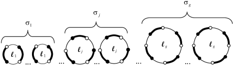
Figure 6: A diagrammatic representation of a compound string belonging to the topology class ${\boldsymbol{\lambda}}=(\ell_{1}^{\sigma_{1}},\cdots,\ell_{g}^{\sigma_{g}})$ with $\sum_{j=1}^{g}\ell_{j}\sigma_{j}=\ell$ and $\sum_{j=1}^{g}\sigma_{j}=r$. Here, $g$ denotes the number of inequivalent parts of the partition ${\boldsymbol{\lambda}}$ whilst $r$ equals the total number of loops.

To calculate the contribution of compound strings to the integral in the l.h.s. of (1.1cghbd), one has to determine (i) the contribution of a diagram belonging to a given topology class to the integral, and (ii) the number of diagrams within a given topology class.

Lemma 5.8. The number of diagrams belonging to the topology class ${\boldsymbol{\lambda}}=(\ell_{1}^{\sigma_{1}},\cdots,\ell_{g}^{\sigma_{g}})$ equals

$${\cal N}_{\{\ell_{1}^{\sigma_{1}},\cdots,\ell_{g}^{\sigma_{g}}\}}=\ell!\prod_{j=1}^{g}\frac{1}{(\ell_{j}!)^{\sigma_{j}}\,\sigma_{j}!}.$$ (1.1cghde)

Proof. To determine the number ${\cal N}_{\{\ell_{1}^{\sigma_{1}},\cdots,\ell_{g}^{\sigma_{g}}\}}$ of diagrams belonging to a given topology class $\{{\bar{\ell}}_{1},\cdots,{\bar{\ell}}_{r}\}=\{\ell_{1}^{\sigma_{1}},\cdots,\ell_{g}^{\sigma_{g}}\}$, we use the multiplication principle.

• First, we distribute the pairs of arguments $\{{\bar{\ell}}_{1},\cdots,{\bar{\ell}}_{r}\}$ between $r$ loops. This can be achieved by $m_{1}$ ways,

  $$m_{1}={\ell\choose{\bar{\ell}}_{1}}\,{\ell-{\bar{\ell}}_{1}\choose{\bar{\ell}}_{2}}\cdots{\ell-{\bar{\ell}}_{1}-\cdots-{\bar{\ell}}_{r-2}\choose{\bar{\ell}}_{r-1}}\,{\ell-{\bar{\ell}}_{1}-\cdots-{\bar{\ell}}_{r-1}\choose{\bar{\ell}}_{r}}\times\frac{1}{r!}.$$

  The factor $1/r!$ reflects the fact that the order of the $r$ loops is irrelevant. (Indeed, a given topology class is associated with an unordered partition of an integer $\ell$). Simple rearrangements show that $m_{1}$ simplifies down to

  $$m_{1}=\frac{\ell!}{{\bar{\ell}}_{1}!\cdots{\bar{\ell}}_{r}!}\frac{1}{r!}.$$ (1.1cghdf)

• Next, we shuffle all inequivalent loops (those with distinct lengths). This can be achieved by $m_{2}$ ways,

  $$m_{2}=\frac{(\sigma_{1}+\cdots+\sigma_{g})!}{\sigma_{1}!\cdots\sigma_{g}!}=\frac{r!}{\sigma_{1}!\cdots\sigma_{g}!}.$$ (1.1cghdg)

As a result, the total number of diagrams belonging to the topology class ${\boldsymbol{\lambda}}=(\ell_{1}^{\sigma_{1}},\cdots,\ell_{g}^{\sigma_{g}})$ equals

$${\cal N}_{\{\ell_{1}^{\sigma_{1}},\cdots,\ell_{g}^{\sigma_{g}}\}}=m_{1}m_{2}=\frac{\ell!}{{\bar{\ell}}_{1}!\cdots{\bar{\ell}}_{r}!}\frac{1}{\sigma_{1}!\cdots\sigma_{g}!}.$$ (1.1cghdh)

The observation $\prod_{j=1}^{r}{\bar{\ell}}_{j}!=\prod_{j=1}^{g}(\ell_{j}!)^{\sigma_{j}}$ ends the proof. $\;\;\;\blacksquare$


Lemma 5.9. A diagram associated with a topology class ${\boldsymbol{\lambda}}=(\ell_{1}^{\sigma_{1}},\cdots,\ell_{g}^{\sigma_{g}})$ contributes

$$C_{\{\ell_{1}^{\sigma_{1}},\cdots,\ell_{g}^{\sigma_{g}}\}}=\prod_{j=1}^{g}C_{L}^{\sigma_{j}}(\ell_{j})$$ (1.1cghdi)

to the integral in the l.h.s. of (1.1cghbd). The function $C_{L}(p)$ is defined by (5.3) of the Corollary 5.3.

Proof. The above claim is a direct consequence of the Lemma 5.2, Definition 5.11, and Remark 5.5. End of proof. $\;\;\;\blacksquare$

Theorem 5.3. All compound strings belonging to the topology class ${\boldsymbol{\lambda}}=(\ell_{1}^{\sigma_{1}},\cdots,\ell_{g}^{\sigma_{g}})$ yield, after the integration in (1.1cghbd), the contribution

$${\tilde{C}}_{{\boldsymbol{\lambda}}}=\frac{\ell!}{(2i)^{\ell}}\prod_{j=1}^{g}\left[\frac{1}{\ell_{j}^{\sigma_{j}}\sigma_{j}!}\left(-\frac{1}{2}\,{\rm tr}_{(0,n-1)}({\boldsymbol{\hat{\upsilon}}}^{\ell_{j}})\right)^{\sigma_{j}}\right].$$ (1.1cghdj)

Proof. Observe that ${\tilde{C}}_{{\boldsymbol{\lambda}}}={\cal N}_{\{\ell_{1}^{\sigma_{1}},\cdots,\ell_{g}^{\sigma_{g}}\}}C_{\{\ell_{1}^{\sigma_{1}},\cdots,\ell_{g}^{\sigma_{g}}\}}$, and make use of (5.3), (1.1cghde) and (1.1cghdi) to derive (1.1cghdj). End of proof. $\;\;\;\blacksquare$

5.5 Proof of the Pfaffian integration theorem

Now we have all ingredients needed to complete the proof of the Pfaffian integration theorem announced in Section 5.1. Indeed, in accordance with the topological interpretation of the terms arising in the Pfaffian expansion (1.1cghx), the integral on the l.h.s. of (1.1cghbd) is given by the sum of contributions of adjacent strings of two types: the longest adjacent strings and the compound strings. The contribution of the former, $C_{L}(\ell)$, is given by the Theorem 5.2 while the contribution of the latter, ${\tilde{C}}_{{\boldsymbol{\lambda}}}$, is determined by the Theorem 5.3. As soon as

$$C_{L}(\ell)={\tilde{C}}_{{\boldsymbol{\lambda}}=(\ell^{1})},$$

one immediately concludes that the integrated Pfaffian equals the sum of ${\tilde{C}}_{\boldsymbol{\lambda}}$ over all unordered partitions ${\boldsymbol{\lambda}}$ of the size $|{\boldsymbol{\lambda}}|=\ell$:

$${\cal I}=\int_{{\mathbb{C}}}\,\prod_{j=1}^{\ell}\,d\pi(z_{j})\,\,{\rm pf\,}\left[\begin{array}[]{cc}Q_{n}(z_{i},z_{j})&Q_{n}(z_{i},{\bar{z}}_{j})\\ Q_{n}({\bar{z}}_{i},z_{j})&Q_{n}({\bar{z}}_{i},{\bar{z}}_{j})\\ \end{array}\right]_{2\ell\times 2\ell}=\sum_{|{\boldsymbol{\lambda}}|=\ell}{\tilde{C}}_{{\boldsymbol{\lambda}}}$$ (1.1cghdm)

$$=\left(\frac{i}{2}\right)^{\ell}(-1)^{\ell}\ell!\,\sum_{|{\boldsymbol{\lambda}}|=\ell}\prod_{j=1}^{g}\left[\frac{1}{\sigma_{j}!}\left(-\frac{1}{2\ell_{j}}\,{\rm tr}_{(0,n-1)}({\boldsymbol{\hat{\upsilon}}}^{\ell_{j}})\right)^{\sigma_{j}}\right].$$ (1.1cghdn)

Quite remarkably, the r.h.s. of (1.1cghdm) can be recognised to be a zonal polynomial (Macdonald 1998)

$$Z_{(1^{\ell})}(p_{1},\cdots,p_{\ell})=(-1)^{\ell}\ell!\sum_{|\boldsymbol{\lambda}|=\ell}\,\prod_{j=1}^{g}\frac{1}{\sigma_{j}!}\left(-\frac{p_{\ell_{j}}}{\ell_{j}}\right)^{\sigma_{j}}$$

with the arguments

$$p_{j}=\frac{1}{2}\,{\rm tr}_{(0,n-1)}({\boldsymbol{\hat{\upsilon}}}^{j}),\;\;\;\;\;j=1,2,\cdots,\ell.$$ (1.1cghdo)

As a result, we conclude that

$${\cal I}=\left(\frac{i}{2}\right)^{\ell}Z_{(1^{\ell})}\left(\frac{1}{2}{\rm tr}_{(0,n-1)}{\boldsymbol{\hat{\upsilon}}}^{1},\cdots,\frac{1}{2}{\rm tr}_{(0,n-1)}{\boldsymbol{\hat{\upsilon}}}^{\ell}\right).$$ (1.1cghdp)

This coincides with the statement (1.1cghbd) of the Pfaffian integration theorem. $\;\;\;\blacksquare$

6 Probability function $p_{n,k}$: General solution and generating function

6.1 General solution

The general solution for the probability function $p_{n,k}$ of a fluctuating number of real eigenvalues in spectra of GinOE is now straightforward to derive. Indeed, it was shown in Section 3.3 that the probability function $p_{n,k}$ admits the representation

$$p_{n,k}=\frac{p_{n,n}}{\ell!}\,\left(\frac{2}{i}\right)^{\ell}\,\prod_{j=1}^{\ell}\int_{{\rm Im\,}z_{j}>0}d^{2}z_{j}\,$$

$$\times\;{\rm erfc}\left(\frac{z_{j}-{\bar{z}}_{j}}{i\sqrt{2}}\right)\,{\rm pf\,}\left[\begin{array}[]{cc}{\cal D}_{n}(z_{i},z_{j})&{\cal D}_{n}(z_{i},{\bar{z}}_{j})\\ {\cal D}_{n}({\bar{z}}_{i},z_{j})&{\cal D}_{n}({\bar{z}}_{i},{\bar{z}}_{j})\\ \end{array}\right]_{2\ell\times 2\ell}$$ (1.1cghc)

with the kernel function ${\cal D}_{n}(x,y)$ given by (1.1cghp) and (1.1cghq).

The $\ell$-fold integral in (6.1) can explicitly be performed by virtue of the Pfaffian integration theorem after the identification

$$d\pi(z)=e^{-(z^{2}+{\bar{z}}^{2})/2}{\rm erfc}\left(\frac{z-{\bar{z}}}{i\sqrt{2}}\right)\,\theta({\rm Im\,}z)\,d^{2}z,\;\;\;\;Q_{n}(x,y)=e^{(x^{2}+y^{2})/2}{\cal D}_{n}(x,y).$$

Straightforward calculations bring

$$p_{n,k}=\frac{p_{n,n}}{\ell!}\,Z_{(1^{\ell})}\left(\frac{1}{2}{\rm tr}_{(0,n-1)}{\boldsymbol{\hat{\upsilon}}}^{1},\cdots,\frac{1}{2}{\rm tr}_{(0,n-1)}{\boldsymbol{\hat{\upsilon}}}^{\ell}\right)$$ (1.1cghd)

where the matrix ${\boldsymbol{\hat{\upsilon}}}$ is given by (1.1cghbf). Combining the definition (1.1cghbf) with (1.1cghaj), (1.1cghao), (1.1cghar), (1.1cghat) and (1.1cghay), one concludes that

$${\boldsymbol{\hat{\upsilon}}}=2i(\boldsymbol{\hat{\mu}}\boldsymbol{\hat{\chi}})=\boldsymbol{{\hat{\sigma}}},$$ (1.1cghe)

see Appendices A and B. Finally, making use of the trace identity

$${\rm tr\,}_{(0,n-1)}{\boldsymbol{\hat{\sigma}}}^{j}=2\,{\rm tr\,}_{(0,\lfloor n/2\rfloor-1)}{\boldsymbol{\hat{\varrho}}}^{j}$$ (1.1cghf)

proven in Appendix C, we end up with the exact formula

$$p_{n,k}=\frac{p_{n,n}}{\ell!}\,Z_{(1^{\ell})}\left({\rm tr\,}_{(0,\lfloor n/2\rfloor-1)}{\boldsymbol{\hat{\varrho}}}^{1},\cdots,{\rm tr\,}_{(0,\lfloor n/2\rfloor-1)}{\boldsymbol{\hat{\varrho}}}^{\ell}\right).$$ (1.1cghg)

The entries of the matrix $\boldsymbol{{\hat{\varrho}}}$, calculated in Appendix C, are given by

$${{\hat{\varrho}}}_{\alpha,\beta}^{{\rm even}} = \int_{0}^{\infty}dy\,y^{2(\beta-\alpha)-1}\,e^{y^{2}}\,{\rm erfc\,}(y\sqrt{2})\,$$ (1.1cghh)

$$\times \left[(2\alpha+1)\,L_{2\alpha+1}^{2(\beta-\alpha)-1}(-2y^{2})+2y^{2}\,L_{2\alpha-1}^{2(\beta-\alpha)+1}(-2y^{2})\right]$$

and

$${\hat{\varrho}}_{\alpha,\,\beta}^{\rm odd}={\hat{\varrho}}_{\alpha,\,\beta}^{\rm even}-(-4)^{m-\beta}\frac{m!}{(2m)!}\frac{(2\beta)!}{\beta!}\,{\hat{\varrho}}_{\alpha,\,m}^{\rm even}$$ (1.1cghi)

for $n=2m$ even and $n=2m+1$ odd, respectively.

6.2 Generating function for $p_{n,k}$

Interestingly, the entire generating function

$$G_{n}(z)=\sum_{\ell=0}^{\lfloor n/2\rfloor}z^{\ell}p_{n,n-2\ell}$$ (1.1cghj)

for the probabilities $p_{n,k}$ can explicitly be determined. To proceed, we make use of the summation formula

$$\sum_{r=0}^{\infty}\frac{z^{r}}{r!}\,Z_{(1^{r})}(p_{1},\cdots,p_{r})=\exp\left(\sum_{r\geq 1}(-1)^{r-1}\frac{p_{r}z^{r}}{r}\right)$$ (1.1cghk)

well known in the theory of symmetric functions (Macdonald 1998). With $p_{r}={\rm tr\,}_{(0,\lfloor n/2\rfloor-1)}{\boldsymbol{\hat{\varrho}}}^{r}$, the r.h.s. transforms to

$$\exp\left({\rm tr\,}_{(0,\lfloor n/2\rfloor-1)}\sum_{r\geq 1}(-1)^{r-1}\frac{(z{\boldsymbol{\hat{\varrho}}})^{r}}{r}\right) =\exp\Big{(}{\rm tr\,}_{(0,\lfloor n/2\rfloor-1)}\log(\boldsymbol{\hat{1}}_{\lfloor n/2\rfloor}+z{\boldsymbol{\hat{\varrho}}})\Big{)},$$ (1.1cghl)

$$=\det\,\left[\boldsymbol{\hat{1}}+z{\boldsymbol{\hat{\varrho}}}\right]_{{\lfloor n/2\rfloor}\times{\lfloor n/2\rfloor}},$$

resulting in an amazingly simple answer:

$$G_{n}(z)=\sum_{\ell=0}^{\lfloor n/2\rfloor}z^{\ell}p_{n,n-2\ell}=p_{n,n}\,\det\,\left[\boldsymbol{\hat{1}}+z{\boldsymbol{\hat{\varrho}}}\right]_{{\lfloor n/2\rfloor}\times{\lfloor n/2\rfloor}}.$$ (1.1cghm)

6.3 Integer moments of the number of real eigenvalues

The result (1.1cghm) allows us to formally determine any integer moment ${\mathbb{E}}[{\cal N}_{r}^{q}]$ of the fluctuating number ${\cal N}_{r}$ of real eigenvalues in the spectra of GinOE. Denoting the fluctuating number of complex eigenvalues through $2{\cal N}_{c}$, we derive:

$${\mathbb{E}}[{\cal N}_{r}^{q}]={\mathbb{E}}[(n-2{\cal N}_{c})^{q}]=\sum_{j=0}^{q}{q\choose j}n^{q-j}(-2)^{j}{\mathbb{E}}[{\cal N}_{c}^{j}].$$ (1.1cghn)

Since

$${\mathbb{E}}[{\cal N}_{c}^{j}]=\left(z\frac{\partial}{\partial z}\right)^{j}\,G_{n}(z)\Big{|}_{z=1},$$ (1.1cgho)

the formula (1.1cghn) simplifies to

$${\mathbb{E}}[{\cal N}_{r}^{q}]=p_{n,n}\,\left(n-2z\frac{\partial}{\partial z}\right)^{q}\,\det\,\left[\boldsymbol{\hat{1}}+z{\boldsymbol{\hat{\varrho}}}\right]_{{\lfloor n/2\rfloor}\times{\lfloor n/2\rfloor}}\Big{|}_{z=1}.$$ (1.1cghp)

Of course, to make the formulae (1.1cghm) and (1.1cghp) explicit, the determinant

$$d_{n}(z)=\det\,\left[\boldsymbol{\hat{1}}+z{\boldsymbol{\hat{\varrho}}}\right]_{{\lfloor n/2\rfloor}\times{\lfloor n/2\rfloor}}$$

has to be evaluated in a closed form. There are a few indications that this is a formidable task, but we have not succeeded in the calculation of $d_{n}(z)$ yet.

7 Asymptotic analysis of the probability $p_{n,n-2}$ to find exactly one pair of complex conjugated eigenvalues

To determine a qualitative behaviour of the probability function $p_{n,k}$, an asymptotic analysis of the exact solution (1.1a) is needed. In this section, the simplest probability function $p_{n,n-2}$,

$$p_{n,n-2}=2\,p_{n,n}\,\int_{0}^{\infty}dy\,y\,e^{y^{2}}\,{\rm erfc}(y\sqrt{2})\,L_{n-2}^{2}(-2y^{2}),$$ (1.1cgha)

is studied in the large-$n$ limit. Our consideration is based on an alternative exact representation for $p_{n,n-2}$ (see the Theorem 7.1) which is more suitable for obtaining regular large-$n$ asymptotics.

7.1 Alternative exact representation of $p_{n,n-2}$

Let us define the sequence

$$S_{n}=\int_{0}^{\infty}dy\,y\,e^{y^{2}}\,{\rm erfc}(y\sqrt{2})\,L_{n}^{2}(-2y^{2}),\;\;\;n=0,1,\cdots,$$ (1.1cghb)

such that

$$p_{n,n-2}=2p_{n,n}\,S_{n-2}.$$ (1.1cghc)

To find an exact alternative representation for $S_{n}$ (and, hence, for $p_{n,n-2}$), we (i) introduce a generating function $\tau(z)$ in the form

$$\tau(z)=\sum_{n=0}^{\infty}S_{n}z^{n}$$ (1.1cghd)

which is supposed to exist in some domain $\Omega_{\tau}\in{\mathbb{R}}$ of the real line ${\mathbb{R}}$ (to be specified later on), (ii) calculate $\tau(z)$ explicitly, and (iii) expand it back in $z\in\Omega_{\tau}$.

Lemma 7.1. The generating function $\tau(z)$ reads:

$$\tau(z)=\frac{1}{2(1-z^{2})(1-z)}\left(-1+\sqrt{2}\sqrt{\frac{1-z}{1-3z}}\right),$$ (1.1cghe)

where

$$-1<z<\frac{1}{3}.$$ (1.1cghf)

Proof. The identity

$$\sum_{n=0}^{\infty}L_{n}^{\lambda}(x)\,z^{n}=(1-z)^{-\lambda-1}\,\exp\left(\frac{xz}{z-1}\right),\;\;\;|z|<1,$$

applied in the context of (1.1cghb) and (1.1cghd), gives rise to the representation

$$\tau(z)=\frac{1}{(1-z)^{3}}\,\int_{0}^{\infty}dy\,y\,{\rm erfc\,}(y\sqrt{2})\,\exp\left(y^{2}\frac{1+z}{1-z}\right),\;\;\;|z|<1.$$ (1.1cghg)

A change of the integration variable $y$ to

$$\xi=y^{2}\frac{1+z}{1-z}$$ (1.1cghh)

followed by integration by parts results in

$$\tau(z)=\frac{1}{2(1-z^{2})(1-z)}\left[e^{\xi}\,{\rm erfc\,}\left(a_{z}\,\sqrt{\xi}\right)\Big{|}_{\xi=0}^{\xi=\infty}-\int_{0}^{\infty}d\xi\,e^{\xi}\,\frac{d}{d\xi}\,{\rm erfc\,}\left(a_{z}\,\sqrt{\xi}\right)\right],$$ (1.1cghi)

where

$$a_{z}=\sqrt{2}\sqrt{\frac{1-z}{1+z}}.$$

For the boundary term in (1.1cghi) to nullify at $\xi=\infty$, the parameter $z$ has to belong to the domain

$$\Omega_{\tau}:\;\;-1<z<\frac{1}{3}.$$ (1.1cghj)

Performing the remaining integral, we end up with (1.1cghe). End of proof. $\;\;\;\blacksquare$

Having determined the generating function $\tau(z)$, we are going to Taylor-expand it around $z=0$ in order to arrive at an alternative formula for the sequence $S_{n}$. As $\tau(z)$ is a relatively simple function, we may expect that $S_{n}$ obtained in this way will also have a relatively simple form.

Lemma 7.2. The following formula holds:

$$S_{n}=\frac{1}{\sqrt{2}}\,\sum_{j=0}^{\lfloor n/2\rfloor}3^{j+\alpha_{n}/2}\,P_{2j+\alpha_{n}}\left(\frac{2}{\sqrt{3}}\right)-\frac{1}{2}\Big{(}\lfloor n/2\rfloor+1\Big{)}.$$ (1.1cghk)

Here, $\alpha_{n}=\lceil n/2\rceil-\lfloor n/2\rfloor$.

Proof. To expand the function $\tau(z)$ given by (1.1cghe) around $z=0$, we represent it in the form

$$\tau(z)=\frac{1}{2}\,\tau_{1}(z)\left(-1+\sqrt{2}\,\tau_{2}(z)\right),$$ (1.1cghl)

where

$$\tau_{1}(z)=\frac{1}{(1-z^{2})(1-z)},\;\;\;\tau_{2}(z)=\sqrt{\frac{1-z}{1-3z}},$$ (1.1cghm)

and constantly use a variant of the Cauchy formula

$$\left(\sum_{k=0}^{\infty}a_{k}\,z^{k}\right)\cdot\left(\sum_{k=0}^{\infty}b_{k}\,z^{k}\right)=\sum_{n=0}^{\infty}c_{n}\,z^{n},\;\;\;\;c_{n}=\sum_{k=0}^{n}a_{k}\,b_{n-k},$$ (1.1cghn)

where absolute convergence of the resulting series is assumed.

Expansion of $\tau_{1}(z)$. To determine the coefficients $c_{k}^{(1)}$ in the expansion

$$\tau_{1}(z)=\sum_{k=0}^{\infty}c_{k}^{(1)}z^{k},$$ (1.1cgho)

we notice that

$$\frac{1}{1-z}=\sum_{k=0}^{\infty}z^{k},\;\;\;\frac{1}{1-z^{2}}=\sum_{k=0}^{\infty}z^{2k},\;\;\;$$ (1.1cghp)

so that, in the notation of (1.1cghn),

$$a_{k}=1,\;\;\;b_{k}=\frac{1+(-1)^{k}}{2}.$$ (1.1cghq)

Straightforward application of the Cauchy formula yields

$$c_{k}^{(1)}=\sum_{j=0}^{k}a_{j}b_{k-j}=\frac{1}{2}\left[k+1+\frac{1+(-1)^{k}}{2}\right]=\lfloor k/2\rfloor+1.$$ (1.1cghr)

Expansion of $\tau_{2}(z)$. To determine the coefficients $c_{k}^{(2)}$ in the expansion

$$\tau_{2}(z)=\sum_{k=0}^{\infty}c_{k}^{(2)}z^{k},$$ (1.1cghs)

we notice that

$$\sqrt{1-z}=\sum_{k=0}^{\infty}{1/2\choose k}\,(-z)^{k},\;\;\;\frac{1}{\sqrt{1-3z}}=\sum_{k=0}^{\infty}{-1/2\choose k}\,(-3z)^{k},\;\;\;$$ (1.1cght)

so that, in the notation of (1.1cghn),

$$a_{k}={1/2\choose k}\,(-1)^{k},\;\;\;b_{k}={-1/2\choose k}\,(-3)^{k}.$$ (1.1cghu)

The Cauchy formula yields

$$c_{k}^{(2)}=\sum_{j=0}^{k}a_{j}b_{k-j}=3^{k}\frac{(1/2)_{k}}{k!}\,\,{}_{2}F_{1}\left(-\frac{1}{2},-k;\frac{1}{2}-k;\frac{1}{3}\right).$$ (1.1cghv)

The latter can be expressed in terms of Legendre polynomials by means of the identity 

$${}_{2}F_{1}\left(-\frac{1}{2},-k;\frac{1}{2}-k;w\right)=\frac{k!}{(1/2)_{k}}\,w^{k/2}\left[P_{k}\left(\frac{w+1}{2\sqrt{w}}\right)-\sqrt{w}\,P_{k-1}\left(\frac{w+1}{2\sqrt{w}}\right)\right]$$ (1.1cghw)

that simplifies (1.1cghv) to

$$c_{k}^{(2)}=3^{k/2}P_{k}\left(\frac{2}{\sqrt{3}}\right)-3^{(k-1)/2}P_{k-1}\left(\frac{2}{\sqrt{3}}\right).$$ (1.1cghx)

Expansion of the product $\tau_{1}(z)\tau_{2}(z)$. To determine the coefficients $c_{k}^{(3)}$ in the expansion

$$\tau_{1}(z)\tau_{2}(z)=\sum_{k=0}^{\infty}c_{k}^{(3)}\,z^{k},$$ (1.1cghy)

we again use the Cauchy formula

$$c_{k}^{(3)}=\sum_{j=0}^{k}c_{k-j}^{(1)}c_{j}^{(2)},$$ (1.1cghz)

with $c_{k}^{(1)}$ and $c_{k}^{(2)}$ given by (1.1cghr) and (1.1cghx), respectively. Lengthy but straightforward calculations result in

$$c_{k}^{(3)}=\sum_{j=0}^{\lfloor k/2\rfloor}3^{j+\alpha_{k}/2}\,P_{2j+\alpha_{k}}\left(\frac{2}{\sqrt{3}}\right),$$ (1.1cghaa)

where $\alpha_{k}=\lceil k/2\rceil-\lfloor k/2\rfloor$.

The observation

$$S_{n}=\frac{1}{\sqrt{2}}\,c_{n}^{(3)}-\frac{1}{2}\,c_{n}^{(1)}$$ (1.1cghab)

completes the proof. $\;\;\;\blacksquare$

Theorem 7.1. The probability $p_{n,n-2}$ to find exactly one pair of complex conjugated eigenvalues in spectra of GinOE admits the following exact representation:

$$p_{n,n-2}=p_{n,n}\,\left[\sqrt{2}\,\sum_{j=0}^{\lfloor n/2\rfloor-1}3^{j+\alpha_{n}/2}\,P_{2j+\alpha_{n}}\left(\frac{2}{\sqrt{3}}\right)-\lfloor n/2\rfloor\right].$$ (1.1cghac)

Here, $\alpha_{n}=\lceil n/2\rceil-\lfloor n/2\rfloor$, and $P_{n}$ stands for Legendre polynomials.

Proof. Use the Lemma 7.2 and relation (1.1cghc) to deduce (1.1cghac). $\;\;\;\blacksquare$

7.2 Asymptotic analysis of $p_{n,n-2}$

The result (1.1cghac), combined with the integral representation of Legendre polynomials

$$P_{n}(\phi)=\frac{1}{\pi}\int_{0}^{\pi}d\theta\left(\phi+\sqrt{\phi^{2}-1}\,\cos\theta\right)^{n},$$ (1.1cghad)

is particularly useful for carrying out an asymptotic analysis of the probability $p_{n,n-2}$ in the large-$n$ limit. Indeed, (1.1cghad) facilitates performing a summation in (1.1cghac) leading to

$$p_{n,n-2}=p_{n,n}\left[\frac{\sqrt{2}}{\pi}\int_{-1}^{+1}\frac{dx}{\sqrt{1-x^{2}}}\,\frac{(x+2)^{\alpha_{n}}-(x+2)^{n}}{1-(x+2)^{2}}-\lfloor n/2\rfloor\right].$$ (1.1cghae)

The large-$n$ behaviour of the integral

$$J_{n}=\int_{-1}^{+1}\frac{dx}{\sqrt{1-x^{2}}}\,\frac{(x+2)^{\alpha_{n}}-(x+2)^{n}}{1-(x+2)^{2}}$$ (1.1cghaf)

is of our primary interest. A saddle-point analysis shows that the saddle point $x_{\rm sp}\approx-2$ lies away from the integration domain $x\in(-1,+1)$. As a result, the contribution of the end points of the integration domain, $x_{\rm L}=-1$ and $x_{\rm R}=+1$, should be examined. One can see that the close vicinity $x=1-\epsilon$ of $x_{\rm R}=+1$ dominates exponentially in $n\gg 1$. Indeed, the vicinity $\epsilon\in(0,c_{0})$ yields

$$J_{n}\approx\int_{0}^{c_{0}}\frac{d\epsilon}{\sqrt{\epsilon(2-\epsilon)}}\,\frac{3^{n}(1-\epsilon/3)^{n}-3^{\alpha_{n}}(1-\epsilon/3)^{\alpha_{n}}}{3^{2}(1-\epsilon/3)^{2}-1},$$

where $c_{0}$ is a proper cut-off. In the large-$n$ limit, only a region of order $n^{-1}$, $\epsilon=\tau/n$, effectively contributes $J_{n}$ reducing it to

$$J_{n}\approx\frac{3^{n}}{8\sqrt{2n}}\int_{0}^{\infty}\frac{d\tau}{\sqrt{\tau}}\,e^{-\tau/3}=\frac{3^{n+1/2}}{8}\sqrt{\frac{\pi}{2n}}.$$ (1.1cghag)

Combined with (1.1cghae) and (1.1cghaf), this estimate leads to the following theorem.

Theorem 7.2. The leading large-$n$ behaviour of the probability $p_{n,n-2}$ is given by the formula

$$p_{n,n-2}\approx\frac{3^{n+1/2}}{8\sqrt{\pi\,n}}\,p_{n,n}$$ (1.1cghah)

where $p_{n,n}=2^{-n(n-1)/4}$.

Remark 7.1. The Theorem 7.2 implies the inequality $p_{n,n-2}\gg p_{n,n}$.

8 Correlations of complex eigenvalues of a matrix without real eigenvalues

8.1 GOE correlations in GinOE spectra

One of the earliest results on eigenlevel statistics in GinOE is due to Ginibre (1965) who spotted that spectra of random real matrices which happened to have no complex eigenvalues exhibit the famous GOE behaviour. Indeed, for ${\boldsymbol{\cal H}}_{n}\in{\mathbb{T}}(n/n)$, the j.p.d.f. (• ‣ 2.3) reduces to

$$P_{{\boldsymbol{\cal H}}_{n}}(\lambda_{1},\cdots,\lambda_{n}) =\frac{2^{-n(n+1)/4}}{n!\,\prod_{j=1}^{n}\Gamma(j/2)}\prod_{i>j=1}^{n}|\lambda_{i}-\lambda_{j}|\,\prod_{j=1}^{n}\,\exp(-\lambda_{j}^{2}/2).$$ (1.1cgha)

The GOE spectral correlations readily follow (Mehta 2004).

8.2 GinSE-like correlations in GinOE spectra

Below, we concentrate on just the opposite case of random real matrices ${\boldsymbol{\cal H}}_{0}\in{\mathbb{T}}(n/0)$ whose spectrum occasionally contains no real eigenvalues. The j.p.d.f. of all complex eigenvalues of ${\boldsymbol{\cal H}}_{0}$ can also be deduced from (• ‣ 2.3), the result being

$$P_{{\boldsymbol{\cal H}}_{0}}(z_{1},\cdots,z_{\ell}) =\frac{2^{-n(n-1)/4}\,i^{n/2}}{(n/2)!\,\prod_{j=1}^{n}\Gamma(j/2)}\,\prod_{i>j=1}^{\ell}|z_{i}-z_{j}|^{2}|z_{i}-{\bar{z}}_{j}|^{2}\,$$ (1.1cghb)

$$\times\prod_{j=1}^{\ell}\,({\bar{z}}_{j}-z_{j})\,{\rm erfc}\left(\frac{z_{j}-{\bar{z}}_{j}}{i\sqrt{2}}\right)\,\exp\left(-\frac{z_{j}^{2}+{\bar{z}}_{j}^{2}}{2}\right)$$

with $n$ even, $n=2\ell$. Remarkably, while the above j.p.d.f. resembles the j.p.d.f. of complex eigenvalues in GinSE (1.1cghc), it is manifestly different from the latter.

Is it possible to determine the correlation functions for the new complex eigenvalue model (1.1cghb)? The answer is positive.

Lemma 8.1. Let ${\boldsymbol{\cal H}_{0}}$ be an $n\times n$ random real matrix with no real eigenvalues such that its entries are statistically independent random variables picked from a normal distribution $\textsf{N}(0,1)$. Then, the $p$-point correlation function ($1\leq p\leq\ell$) of its complex eigenvalues equals

$$R^{({\boldsymbol{\cal H}}_{0})}_{0,p}(z_{1},\cdots,z_{p};n)=p_{n,n}\,\frac{\prod_{j=0}^{\ell-1}r_{j}}{\prod_{j=1}^{n}\Gamma(j/2)}\prod_{j=1}^{p}{\rm erfc}\left(\frac{z_{j}-{\bar{z}}_{j}}{i\sqrt{2}}\right)\,\exp\left(-\frac{z_{j}^{2}+{\bar{z}}_{j}^{2}}{2}\right)$$

$$\times\,{\rm pf\,}\left[\begin{array}[]{cc}\kappa_{\ell}(z_{i},z_{j})&\kappa_{\ell}(z_{i},{\bar{z}}_{j})\\ \kappa_{\ell}({\bar{z}}_{i},z_{j})&\kappa_{\ell}({\bar{z}}_{i},{\bar{z}}_{j})\\ \end{array}\right]_{2p\times 2p}.$$ (1.1cghe)

Here, $n=2\ell$ and the ‘pre-kernel’ $\kappa_{\ell}$ is

$$\kappa_{\ell}(z,z^{\prime})=i\sum_{j=0}^{\ell-1}\frac{1}{r_{j}}\bigg{[}p_{2j}(z)p_{2j+1}(z^{\prime})-p_{2j}(z^{\prime})p_{2j+1}(z)\bigg{]}.$$ (1.1cghf)

The polynomials $p_{j}(z)$ in (1.1cghf) are skew orthogonal in the complex half-plane ${\rm Im\,}z>0$,

$$\langle p_{2j+1},p_{2k}\rangle_{\rm c}=-\langle p_{2k},p_{2j+1}\rangle_{\rm c}=i\,r_{j}\,\delta_{jk},$$ (1.1cghg)

$$\langle p_{2j+1},p_{2k+1}\rangle_{\rm c}=\langle p_{2j},p_{2k}\rangle_{\rm c}=0,$$ (1.1cghh)

with respect to the skew product

$$\langle f,g\rangle_{\rm c}=\int_{{\rm Im\,}z>0}d^{2}z\,{\rm erfc}\left(\frac{z-{\bar{z}}}{i\sqrt{2}}\right)\,\exp\left(-\frac{z^{2}+{\bar{z}}^{2}}{2}\right)\,\left[f(z)g({\bar{z}})-f({\bar{z}})g(z)\right].$$ (1.1cghi)

Proof. By definition (2.3), the $p$-point correlation function is

$$R^{({\boldsymbol{\cal H}}_{0})}_{0,p}(z_{1},\cdots,z_{p};n)=\frac{\ell!}{(\ell-p)!}\prod_{j=p+1}^{\ell}\int_{{\rm Im}z_{j}>0}d^{2}z_{j}\,P_{{\boldsymbol{\cal H}}_{0}}(z_{1},\cdots,z_{\ell}).$$ (1.1cghj)

Since the $n\times n$ real matrix with no real eigenvalues has $\ell$ pairs of complex conjugated eigenvalues, it holds that $n=2\ell$.

Conceptually, the proof to be presented consists of three parts. First, we concentrate on the j.p.d.f. $P_{{\boldsymbol{\cal H}}_{0}}(z_{1},\cdots,z_{\ell})$ and show that it can be represented in terms of a certain quaternion determinant. Second, we prove that the quaternion matrix under the quaternion determinant enjoys the projection property (see Definition 2.1). Third, we apply the Dyson integration theorem to carry out all $(\ell-p)$ integrations in (1.1cghj).

Part 1.—As the Vandermonde structure of (1.1cghb) mimics that of GinSE (1.1cghc), it is tempting to employ the identity

$$\prod_{i>j=1}^{\ell}|z_{i}-z_{j}|^{2}|z_{i}-{\bar{z}}_{j}|^{2}\,\prod_{j=1}^{\ell}({\bar{z}_{j}-z_{j}})=\det\big{[}z_{j}^{i-1},\,{\bar{z}}_{j}^{i-1}\big{]}_{\matrix{\scriptstyle i=1,\cdots,2\ell\hfill\cr\scriptstyle j=1,\cdots,\ell\hfill\cr}}$$ (1.1cghk)

that helps us reduce the j.p.d.f. $P_{{\boldsymbol{\cal H}}_{0}}$ to the form

$$P_{{\boldsymbol{\cal H}}_{0}}(z_{1},\cdots,z_{\ell}) =\frac{2^{-n(n-1)/4}\,i^{\ell}}{(n/2)!\,\prod_{j=1}^{n}\Gamma(j/2)}\,\det\big{[}p_{i-1}(z_{j}),\,p_{i-1}({\bar{z}}_{j})\big{]}_{\matrix{\scriptstyle i=1,\cdots,2\ell\hfill\cr\scriptstyle j=1,\cdots,\ell\hfill\cr}}$$ (1.1cghl)

$$\times\prod_{j=1}^{\ell}{\rm erfc}\left(\frac{z_{j}-{\bar{z}}_{j}}{i\sqrt{2}}\right)\,\exp\left(-\frac{z_{j}^{2}+{\bar{z}}_{j}^{2}}{2}\right).$$

Here, $p_{k}(z)$ are arbitrary monic polynomials of degree $k$.

The very structure of the matrix under the determinant in (1.1cghl),

$$\det\,\left[\begin{array}[]{cccccc}p_{0}(z_{1})&p_{0}({\bar{z}}_{1})&\cdots&\cdots&p_{0}(z_{\ell})&p_{0}({\bar{z}}_{\ell})\\ p_{1}(z_{1})&p_{1}({\bar{z}}_{1})&\cdots&\cdots&p_{1}(z_{\ell})&p_{1}({\bar{z}}_{\ell})\\ \vdots&\vdots&{}\hfil&{}\hfil&\vdots&\vdots\\ \vdots&\vdots&{}\hfil&{}\hfil&\vdots&\vdots\\ p_{2\ell-2}(z_{1})&p_{2\ell-2}({\bar{z}}_{1})&\cdots&\cdots&p_{2\ell-2}(z_{\ell})&p_{2\ell-2}({\bar{z}}_{\ell})\\ p_{2\ell-1}(z_{1})&p_{2\ell-1}({\bar{z}}_{1})&\cdots&\cdots&p_{2\ell-1}(z_{\ell})&p_{2\ell-1}({\bar{z}}_{\ell})\\ \end{array}\right]$$ (1.1cghs)

suggests that we introduce a set of quaternions $\{{\boldsymbol{\psi}}_{0}(z),\cdots,{\boldsymbol{\psi}}_{\ell-1}(z)\}$,

$${\boldsymbol{\psi}}_{j}(z) =\frac{p_{2j}(z)+p_{2j+1}(\bar{z})}{2}\,{\boldsymbol{\hat{e}}_{0}}+\frac{p_{2j}(z)-p_{2j+1}(\bar{z})}{2i}\,{\boldsymbol{\hat{e}}_{1}}$$ (1.1cght)

$$+\frac{p_{2j}(\bar{z})-p_{2j+1}(z)}{2}\,{\boldsymbol{\hat{e}}_{2}}+\frac{p_{2j}(\bar{z})+p_{2j+1}(z)}{2i}\,{\boldsymbol{\hat{e}}_{3}}$$

whose $2\times 2$ matrix representation reads

$$\Theta[{\boldsymbol{\psi}}_{j}(z)]=\left[\begin{array}[]{cc}p_{2j}(z)&p_{2j}({\bar{z}})\\ p_{2j+1}(z)&p_{2j+1}({\bar{z}})\\ \end{array}\right].$$ (1.1cghaf)

As a result, the above determinant can equivalently be written as

$$\det\,\left[p_{i-1}(z_{j}),\,p_{i-1}({\bar{z}}_{j})\right]_{\matrix{\scriptstyle i=1,\cdots,2\ell\hfill\cr\scriptstyle j=1,\cdots,\ell\hfill\cr}}=\det\,\left[\Theta[{\boldsymbol{\psi}}_{i-1}(z_{j})]\right]_{\matrix{\scriptstyle i=1,\cdots,\ell\hfill\cr\scriptstyle j=1,\cdots,\ell\hfill\cr}}.$$ (1.1cghag)

The latter can be put into a quaternion determinant form (see Corollary 5.1.3 in Mehta’s book (2004)):

$$\det\,\left[\Theta[{\boldsymbol{\psi}}_{i-1}(z_{j})]\right]_{\matrix{\scriptstyle i=1,\cdots,\ell\hfill\cr\scriptstyle j=1,\cdots,\ell\hfill\cr}}={\rm qdet\,}\left[\boldsymbol{{\cal A}\bar{{\cal A}}}\,\right]_{\ell\times\ell}={\rm qdet\,}\left[\boldsymbol{\bar{{\cal A}}{\cal A}}\,\right]_{\ell\times\ell}.$$ (1.1cghah)

Here, $\boldsymbol{{\cal A}}$ is an $\ell\times\ell$ quaternion matrix with the entries

$$\boldsymbol{{\cal A}}_{ij}={\boldsymbol{\psi}}_{i-1}(z_{j})$$ (1.1cghai)

and $\boldsymbol{{\bar{\cal A}}}$ is the dual quaternion matrix whose entries

$$\boldsymbol{\bar{{\cal A}}}_{ij}={\boldsymbol{\bar{\psi}}}_{j-1}(z_{i})$$ (1.1cghaj)

are determined by the dual quaternion $\bar{{\boldsymbol{\psi}}}_{j}(z)$,

$${\bar{\boldsymbol{\psi}}}_{j}(z) =\frac{p_{2j}(z)+p_{2j+1}(\bar{z})}{2}\,{\boldsymbol{\hat{e}}_{0}}-\frac{p_{2j}(z)-p_{2j+1}(\bar{z})}{2i}\,{\boldsymbol{\hat{e}}_{1}}$$ (1.1cghak)

$$-\frac{p_{2j}(\bar{z})-p_{2j+1}(z)}{2}\,{\boldsymbol{\hat{e}}_{2}}-\frac{p_{2j}(\bar{z})+p_{2j+1}(z)}{2i}\,{\boldsymbol{\hat{e}}_{3}}$$

such that

$$\Theta[{\boldsymbol{\bar{\psi}}}_{j}(z)]=\boldsymbol{{\hat{e}}}_{2}\,\Theta[{\boldsymbol{\psi}}_{j}(z)]^{\rm T}\,\boldsymbol{{\hat{e}}}_{2}^{-1}=\left[\begin{array}[]{cc}p_{2j+1}(\bar{z})&-p_{2j}({\bar{z}})\\ -p_{2j+1}(z)&p_{2j}(z)\\ \end{array}\right].$$ (1.1cghan)

Combining (1.1cghag) and (1.1cghah) into

$$\det\,\left[p_{i-1}(z_{j}),\,p_{i-1}({\bar{z}}_{j})\right]_{\matrix{\scriptstyle i=1,\cdots,2\ell\hfill\cr\scriptstyle j=1,\cdots,\ell\hfill\cr}}={\rm qdet\,}\left[\boldsymbol{\bar{{\cal A}}{\cal A}}\,\right]_{\ell\times\ell},$$ (1.1cghao)

we obtain

$$\det\,\left[p_{i-1}(z_{j}),\,p_{i-1}({\bar{z}}_{j})\right]_{\matrix{\scriptstyle i=1,\cdots,2\ell\hfill\cr\scriptstyle j=1,\cdots,\ell\hfill\cr}}=i^{-\ell}\prod_{j=0}^{\ell-1}r_{j}\;{\rm qdet}\left[{\boldsymbol{\hat{\kappa}}}_{\ell}(z_{i},z_{j})\right]_{\ell\times\ell}.$$ (1.1cghap)

Here, the (self-dual) quaternion kernel ${\boldsymbol{\hat{\kappa}}}_{\ell}$ admits a $2\times 2$ matrix representation

$$\Theta\left[{\boldsymbol{\hat{\kappa}}}_{\ell}(z_{i},z_{j})\right]=\left(\begin{array}[]{cc}-\kappa_{\ell}({\bar{z}}_{i},z_{j})&-\kappa_{\ell}({\bar{z}}_{i},{\bar{z}}_{j})\\ \kappa_{\ell}(z_{i},z_{j})&\kappa_{\ell}(z_{i},\bar{z}_{j})\\ \end{array}\right)$$ (1.1cghas)

with

$$\kappa_{\ell}(z,w)=i\sum_{j=0}^{\ell-1}\frac{1}{r_{j}}\bigg{[}p_{2j}(z)p_{2j+1}(w)-p_{2j}(w)p_{2j+1}(z)\bigg{]}.$$ (1.1cghat)

The set of constants $\{r_{j}\}$ is not fixed so far.

The above consideration results in the following expression for the j.p.d.f. $P_{{\boldsymbol{\cal H}}_{0}}$ [Eq. (1.1cghl)]

$$P_{{\boldsymbol{\cal H}}_{0}}(z_{1},\cdots,z_{\ell}) =\frac{2^{-n(n-1)/4}}{(n/2)!}\,\frac{\prod_{j=0}^{\ell-1}r_{j}}{\prod_{j=1}^{n}\Gamma(j/2)}\;{\rm qdet}\left[{\boldsymbol{\hat{\kappa}}}_{\ell}(z_{i},z_{j})\right]_{\ell\times\ell}$$ (1.1cghau)

$$\times\prod_{j=1}^{\ell}{\rm erfc}\left(\frac{z_{j}-{\bar{z}}_{j}}{i\sqrt{2}}\right)\,\exp\left(-\frac{z_{j}^{2}+{\bar{z}}_{j}^{2}}{2}\right),$$

that serves as a proper starting point for evaluating the $p$-point correlation function $R^{{({\boldsymbol{\cal H}}_{0})}}_{0,p}(z_{1},\cdots,z_{p};n)$ specified in Eq. (8.2).

Part 2.—Now, we are going to prove that the quaternion ${\boldsymbol{\hat{\kappa}}}_{\ell}$ satisfies the projection property Definition 2.1. To simplify the consideration to follow, we set the so far arbitrary monic polynomials $p_{k}(z)$ to be skew-orthogonal in the complex half-plane, ${\rm Im\,}z>0$, as defined by (1.1cghg) – (1.1cghi).

Having imposed the skew-orthogonality on $p_{k}(z)$, with $r_{j}\in{\mathbb{R}}$, we are in the position to verify whether or not the projection property for the quaternion ${\boldsymbol{\hat{\kappa}}}_{\ell}$ is fulfilled. In accordance with the Definition 2.1, one has to consider the integral

$$I=\int_{{\rm Im\,}w>0}d^{2}w\,{\rm erfc}\left(\frac{w-{\bar{w}}}{i\sqrt{2}}\right)\,\exp\left(-\frac{w^{2}+{\bar{w}}^{2}}{2}\right)\,\Theta\left[{\boldsymbol{\hat{\kappa}}}_{\ell}(z_{1},w)\right]\,\Theta\left[{\boldsymbol{\hat{\kappa}}}_{\ell}(w,z_{2})\right]$$ (1.1cghav)

that equals

$$I=\left(\begin{array}[]{cc}\delta_{\ell}({\bar{z}}_{1},z_{2})&\delta_{\ell}({\bar{z}}_{1},{\bar{z}}_{2})\\ -\delta_{\ell}(z_{1},z_{2})&-\delta_{\ell}(z_{1},\bar{z}_{2})\\ \end{array}\right).$$ (1.1cghay)

Here, the function $\delta_{\ell}(z_{1},z_{2})$ is defined by the integral

$$\delta_{\ell}(z_{1},z_{2})=\int_{{\rm Im\,}w>0}d^{2}w\,{\rm erfc}\left(\frac{w-{\bar{w}}}{i\sqrt{2}}\right)\,\exp\left(-\frac{w^{2}+{\bar{w}}^{2}}{2}\right)\,$$

$$\times\big{[}\kappa_{\ell}(z_{1},w)\kappa_{\ell}({\bar{w}},z_{2})-\kappa_{\ell}(z_{2},w)\kappa_{\ell}({\bar{w}},z_{1})\big{]}.$$ (1.1cghaz)

Its evaluation, based on (1.1cghat), (1.1cghi), (1.1cghg) and (1.1cghh), is straightforward, the result being

$$\delta_{\ell}(z_{1},z_{2})=-\kappa_{\ell}(z_{1},z_{2})$$ (1.1cghba)

so that

$$I=\Theta\left[{\boldsymbol{\hat{\kappa}}}_{\ell}(z_{1},z_{2})\right].$$ (1.1cghbb)

Put differently, the quaternion kernel ${\boldsymbol{\hat{\kappa}}}_{\ell}$ satisfies the projection property in the form

$$\int_{{\rm Im\,}w>0}d^{2}w\,{\rm erfc}\left(\frac{w-{\bar{w}}}{i\sqrt{2}}\right)\,\exp\left(-\frac{w^{2}+{\bar{w}}^{2}}{2}\right)\,{\boldsymbol{\hat{\kappa}}}_{\ell}(z_{1},w)\,{\boldsymbol{\hat{\kappa}}}_{\ell}(w,z_{2})={\boldsymbol{\hat{\kappa}}}_{\ell}(z_{1},z_{2}).$$ (1.1cghbc)

This is precisely (1.1cghhb) of the Dyson integration theorem with a quaternion $\lambda=0$.

Part 3.—The above proof of the projection property for the quaternion kernel ${\boldsymbol{\hat{\kappa}}}_{\ell}$ in (1.1cghau) paves the way for carrying out the $(\ell-p)$ integrations in (1.1cghj). Indeed, the integrations therein can be performed by virtue of the Dyson integration theorem (Theorem 2.1) since

$$\Theta\left[{\bar{\boldsymbol{\hat{\kappa}}}}_{\ell}(z_{1},z_{2})\right]\stackrel{{\scriptstyle\rm def}}{{=}}{\boldsymbol{\hat{e}}}_{2}\,\Theta\left[{\boldsymbol{\hat{\kappa}}}_{\ell}(z_{1},z_{2})\right]^{\rm T}{\boldsymbol{\hat{e}}}_{2}^{-1}=\Theta\left[{\boldsymbol{\hat{\kappa}}}_{\ell}(z_{2},z_{1})\right].$$ (1.1cghbd)

To this end, one has to determine the constant $c$ defined by the integral [see (1.1cghhd)]

$$c\,{\boldsymbol{e}_{0}}=\int_{{\rm Im\,}z>0}d^{2}z\,{\rm erfc}\left(\frac{z-{\bar{z}}}{i\sqrt{2}}\right)\,\exp\left(-\frac{z^{2}+{\bar{z}}^{2}}{2}\right)\,{\boldsymbol{\hat{\kappa}}}_{\ell}(z,z)$$ (1.1cghbe)

yielding

$$c=\int_{{\rm Im\,}z>0}d^{2}z\,{\rm erfc}\left(\frac{z-{\bar{z}}}{i\sqrt{2}}\right)\,\exp\left(-\frac{z^{2}+{\bar{z}}^{2}}{2}\right)\,{\kappa}_{\ell}(z,\bar{z})=\ell.$$ (1.1cghbf)

The projection property (1.1cghbc) combined with the result (1.1cghbf) brings the key integration identity:

$$\frac{1}{(\ell-p)!}\prod_{j=p+1}^{\ell}\int_{{\rm Im\,}z_{j}>0}d^{2}z_{j}\,{\rm erfc}\left(\frac{z_{j}-{\bar{z}}_{j}}{i\sqrt{2}}\right)\,\exp\left(-\frac{z_{j}^{2}+{\bar{z}}_{j}^{2}}{2}\right)\,{\rm qdet}\left[{\boldsymbol{\hat{\kappa}}}_{\ell}(z_{i},z_{j})\right]_{\ell\times\ell}$$

$$={\rm qdet}\left[{\boldsymbol{\hat{\kappa}}}_{\ell}(z_{i},z_{j})\right]_{p\times p}={\rm pf\,}\left[\begin{array}[]{cc}{\kappa}_{\ell}(z_{i},z_{j})&{\kappa}_{\ell}(z_{i},{\bar{z}}_{j})\\ {\kappa}_{\ell}({\bar{z}}_{i},z_{j})&{\kappa}_{\ell}({\bar{z}}_{i},{\bar{z}}_{j})\\ \end{array}\right]_{2p\times 2p}.$$ (1.1cghbi)

Applied to (1.1cghj) and (1.1cghau), it results in

$$R^{({\boldsymbol{\cal H}}_{k})}_{0,p}(z_{1},\cdots,z_{p};n)=p_{n,n}\,\frac{\prod_{j=0}^{\ell-1}r_{j}}{\prod_{j=1}^{n}\Gamma(j/2)}\;\prod_{j=1}^{p}{\rm erfc}\left(\frac{z_{j}-{\bar{z}}_{j}}{i\sqrt{2}}\right)\,\exp\left(-\frac{z_{j}^{2}+{\bar{z}}_{j}^{2}}{2}\right)$$

$$\times{\rm pf\,}\left[\begin{array}[]{cc}{\kappa}_{\ell}(z_{i},z_{j})&{\kappa}_{\ell}(z_{i},{\bar{z}}_{j})\\ {\kappa}_{\ell}({\bar{z}}_{i},z_{j})&{\kappa}_{\ell}({\bar{z}}_{i},{\bar{z}}_{j})\\ \end{array}\right]_{2p\times 2p},$$ (1.1cghbl)

where $n=2\ell$. This completes the proof of the Lemma 8.1. $\;\;\;\blacksquare$

8.3 Probability $p_{n,0}$ to find no real eigenvalues

The technique exposed in the previous subsection allows us to establish the following structural result for the probability to find no real eigenvalues in GinOE spectra.

Corollary 8.1. The probability $p_{n,0}$ to find no real eigenvalues in spectra of GinOE equals

$$p_{n,0}=\frac{p_{n,n}}{\prod_{j=1}^{n}\Gamma(j/2)}\,\prod_{j=0}^{\ell-1}r_{j}.$$ (1.1cghbm)

Here, $n=2\ell$; the constants $r_{j}$ are defined by (1.1cghg).

Proof. For $n=2\ell$ even, the definition (1.1cgha) translates to

$$p_{n,0}=\prod_{j=1}^{\ell}\int_{{\rm Im\,}z_{j}>0}d^{2}z_{j}\,P_{{\boldsymbol{\cal H}_{0}}}(z_{1},\cdots,z_{\ell}).$$ (1.1cghbn)

Given $P_{{\boldsymbol{\cal H}_{0}}}$ in the form (1.1cghau), the above probability reduces to

$$p_{n,0}=\frac{p_{n,n}}{\ell!}\,\frac{\prod_{j=0}^{\ell-1}r_{j}}{\prod_{j=1}^{n}\Gamma(j/2)}\,\prod_{j=1}^{\ell}\int_{{\rm Im\,}z_{j}>0}d^{2}z_{j}\;{\rm qdet}\left[{\boldsymbol{\hat{\kappa}}}_{\ell}(z_{i},z_{j})\right]_{\ell\times\ell}$$

$$\times\prod_{j=1}^{\ell}{\rm erfc}\left(\frac{z_{j}-{\bar{z}}_{j}}{i\sqrt{2}}\right)\,\exp\left(-\frac{z_{j}^{2}+{\bar{z}}_{j}^{2}}{2}\right).$$ (1.1cghbo)

Due to the projection property (1.1cghbc) of the quaternion kernel ${\boldsymbol{\hat{\kappa}}}_{\ell}$, the integration in (8.3) can readily be performed [see, e.g., the identity (8.2)] bringing

$$\prod_{j=1}^{\ell}\int_{{\rm Im\,}z_{j}>0}d^{2}z_{j}\;{\rm qdet}\left[{\boldsymbol{\hat{\kappa}}}_{\ell}(z_{i},z_{j})\right]_{\ell\times\ell}\,\prod_{j=1}^{\ell}{\rm erfc}\left(\frac{z_{j}-{\bar{z}}_{j}}{i\sqrt{2}}\right)\,\exp\left(-\frac{z_{j}^{2}+{\bar{z}}_{j}^{2}}{2}\right)=\ell!$$ (1.1cghbp)

This establishes the result (1.1cghbm) thus completing the proof. $\;\;\;\blacksquare$

Remark 8.1. To make the formula (1.1cghbm) explicit, one has to know the normalisation constants $r_{j}$ which we have failed to determine explicitly so far.

9 Conclusions and open problems

To summarise, an exact formula was derived for the probability $p_{n,k}$ to find precisely $k$ real eigenvalues in the spectrum of an $n\times n$ random matrix drawn from GinOE. Based on the Pfaffian integration theorem (that can be seen as an extension of the Dyson integration theorem to kernels that do not possess the projection property), the solution found expresses the probability function $p_{n,k}$ in terms of zonal polynomials . This links the integrable structure of GinOE to the theory of symmetric functions (Macdonald 1998). Undoubtedly, much more effort is needed to accomplish the spectral theory of GinOE. Below, we list some of the open problems that have to be addressed.

(I) Probability Function $p_{n,k}$ and Associated Generating Function $G_{n}(z)$. The exact solution for the probability $p_{n,k}$ expresses the probability in terms of zonal polynomials of some complicated arguments. Does a more explicit representation (like the one for $p_{n,n-2}$, see (1.1cgha) and (1.1cghac)) exist for $p_{n,k}$? A similar question arises in the context of the solution for the determinantal generating function $G_{n}(z)$ given by (1.1cghm). Can the determinant (1.1cghm) be calculated in a closed form as a function of $k$, $n$ and $z$? We have a few indications that this is a formidable task.

(II) Asymptotic Analysis of $p_{n,k}$ in the Large-$n$ Limit. The problem we wish to pose here concerns the large-$n$ behaviour of $p_{n,k}$ in various scaling limits: (a) $k\sim n^{0}$, (b) $n-k\sim n^{0}$, and (c) $k\sim n^{1/2}$ (this scaling is prompted by the result (1.1cgham) for an average number of real eigenvalues). If available, the large-$n$ formulae of this kind would facilitate a comparison of our exact theory with existing numerical and experimental data, as reported by Halasz et al (1997) and Kwapień et al (2000).

(III) Correlation Functions of Complex Eigenvalues and $p_{n,0}$. The solution presented for these two spectral characteristics involves specific polynomials which are skew orthogonal in the complex plane with respect to a somewhat unusual weight function containing the complementary error function. Can those be determined explicitly to eventually bring closed formulae for both the correlation functions and the probability $p_{n,0}$? Their large-$n$ analysis would be of great interest, too.

(IV) Correlation Functions of Both Real and Complex Eigenvalues and a Generalised Pfaffian Integration Theorem. The calculation of all partial $(p,q)$-point correlation functions $R_{p,q}^{({\boldsymbol{\cal H}}_{k})}$ for GinOE matrices with a given number $(k)$ of real eigenvalues (defined as an integral of the j.p.d.f. over all but $p$ real and $q$ complex eigenvalues, see (2.3)) is yet another important problem to tackle. Also, can the unconditional $(p,q)$-point correlation functions $R_{p,q}=\sum_{k}R_{p,q}^{({\boldsymbol{\cal H}}_{k})}$ be explicitly determined? We believe that progress in this direction can be achieved through a proper extension of the Pfaffian integration theorem:

$$\prod_{j=p+1}^{\ell}\,\int_{z_{j}\in{\mathbb{C}}}d\pi(z_{j})\,\, {\rm pf\,}\left[\begin{array}[]{cc}Q_{n}(z_{i},z_{j})&Q_{n}(z_{i},{\bar{z}}_{j})\\ Q_{n}({\bar{z}}_{i},z_{j})&Q_{n}({\bar{z}}_{i},{\bar{z}}_{j})\\ \end{array}\right]_{2\ell\times 2\ell}=\;?$$ (1.1cghc)

Here, the notation of the Theorem 5.1 was used. Notice that one should not assume the projection property for the kernel $Q_{n}$.

The above list of open problems calls for further research of GinOE that will eventually unveil the rich mathematical structures underlying this classical but still largely unexplored non-Hermitean random matrix model.

Appendix A. The $n\times n$ matrix ${\boldsymbol{\hat{\chi}}}$

A1. Symmetries of ${\boldsymbol{\hat{\chi}}}$ and useful expansions.—The definition (1.1cghay) of the matrix ${\boldsymbol{\hat{\chi}}}$ suggests that it is antisymmetric,

$${\hat{\chi}}_{jk}=-{\hat{\chi}}_{kj},$$ (A.4)

and purely imaginary

$${\bar{\hat{\chi}}}_{jk}=-{\hat{\chi}}_{jk}$$ (A.5)

as confirmed by the formula

$${\hat{\chi}}_{jk}=i\int d\alpha(w)\,e^{-(w^{2}+{\bar{w}}^{2})/2}\,\left[\,{\rm Re\,}q_{j}(w)\,{\rm Im\,}q_{k}({\bar{w}})+{\rm Im\,}q_{j}(w)\,{\rm Re\,}q_{k}({\bar{w}})\right].$$ (A.6)

Due to (3.2) that relates the skew orthogonal polynomials $q_{j}(w)$ to Hermite polynomials $H_{j}(w)$, the following expansions are useful for even/odd order Hermite polynomials taken at $w=x+iy$:

$${\rm Re\,}H_{2m}(w)=\sum_{j=0}^{m}\frac{(-1)^{j}2^{2j}}{(2j)!}\,(-2m)_{2j}\,y^{2j}H_{2m-2j}(x),$$ (A.7)

$${\rm Im\,}H_{2m}(w)=\sum_{j=0}^{m-1}\frac{(-1)^{j-1}2^{2j+1}}{(2j+1)!}\,(-2m)_{2j+1}\,y^{2j+1}H_{2m-2j-1}(x),$$ (A.8)

and

$${\rm Re\,}H_{2m+1}(w)=\sum_{j=0}^{m}\frac{(-1)^{j}2^{2j}}{(2j)!}\,(-2m-1)_{2j}\,y^{2j}H_{2m+1-2j}(x),$$ (A.9)

$${\rm Im\,}H_{2m+1}(w)=\sum_{j=0}^{m}\frac{(-1)^{j-1}2^{2j+1}}{(2j+1)!}\,(-2m-1)_{2j+1}\,y^{2j+1}H_{2m-2j}(x).$$ (A.10)

Here, $(-a)_{n}$ is the Pochhammer symbol ($a>0$),

$$(-a)_{n}=(-1)^{n}\frac{\Gamma(a+1)}{\Gamma(a-n+1)}.$$

A2. Calculation of the matrix elements ${\hat{\chi}}_{2\alpha,2\beta}$ and ${\hat{\chi}}_{2\alpha+1,2\beta+1}$.—We claim that

$${\hat{\chi}}_{2\alpha,2\beta}={\hat{\chi}}_{2\alpha+1,2\beta+1}=0$$ (A.11)

for all $\alpha=0,1,\cdots$ and $\beta=0,1,\cdots$. To prove this statement, let us consider ${\hat{\chi}}_{2\alpha,2\beta}$. In accordance with (A.6), this matrix element is related to the integral containing

$$e^{-(w^{2}+{\bar{w}}^{2})/2}\,\Big{[}{\rm Re\,}q_{2\alpha}(w)\,{\rm Im\,}q_{2\beta}({\bar{w}})+{\rm Im\,}q_{2\alpha}(w)\,{\rm Re\,}q_{2\beta}({\bar{w}})\Big{]}.$$

Having in mind (3.2), (A.7) and (A.8), we observe that the above expression, being integrated over the $x$-part of the integration measure

$$d\alpha(w)=dx\,\cdot{\rm erfc}(y\sqrt{2})\,\theta(y)\,dy,$$ (A.12)

nullifies due to the products of Hermite polynomials $H_{{\rm even}\,\natural}(x)\,H_{{\rm odd}\,\natural}(x)$ of even and odd orders. Thus, we conclude that ${\hat{\chi}}_{2\alpha,2\beta}=0$. By the same token, the matrix element ${\hat{\chi}}_{2\alpha+1,2\beta+1}$ is zero as well.

A3. Calculation of the matrix elements ${\hat{\chi}}_{2\alpha+1,2\beta}$ and ${\hat{\chi}}_{2\alpha,2\beta+1}$.—We claim that

$${\hat{\chi}}_{2\alpha+1,2\beta}=\frac{i}{2}\,(-1)^{\beta-\alpha}h_{\alpha}\,\int_{0}^{\infty}dy\,y^{2(\beta-\alpha)-1}\,e^{y^{2}}\,{\rm erfc\,}(y\sqrt{2})\,$$

$$\times\left[(2\alpha+1)\,L_{2\alpha+1}^{2(\beta-\alpha)-1}(-2y^{2})+2y^{2}\,L_{2\alpha-1}^{2(\beta-\alpha)+1}(-2y^{2})\right].$$ (A.13)

In accordance with the symmetry relation (A.4), it holds

$${\hat{\chi}}_{2\alpha,2\beta+1}=-{\hat{\chi}}_{2\beta+1,2\alpha}.$$ (A.14)

To prove the result (Appendix A. The $n\times n$ matrix ${\boldsymbol{\hat{\chi}}}$), we start with the definition (A.6),

$${\hat{\chi}}_{2\alpha+1,2\beta}=i\int d\alpha(w)\,e^{-(w^{2}+{\bar{w}}^{2})/2}\,$$

$$\times\left[\,{\rm Re\,}q_{2\alpha+1}(w)\,{\rm Im\,}q_{2\beta}({\bar{w}})+{\rm Im\,}q_{2\alpha+1}(w)\,{\rm Re\,}q_{2\beta}({\bar{w}})\right],$$ (A.15)

where the skew orthogonal polynomials $q_{j}(w)$ are given by (3.2). Substituting them into (Appendix A. The $n\times n$ matrix ${\boldsymbol{\hat{\chi}}}$), representing $w$ as $w=x+iy$ and making use of the expansions (A.7) to (A.10), one can carry out the integration over $x\in{\mathbb{R}}$ straightforwardly, due to the factorised integration measure (A.12) and the orthogonality of Hermite polynomials on ${\mathbb{R}}$ with respect to the weight $\exp(-x^{2})$. Lengthy but straightforward calculations result in

$${\hat{\chi}}_{2\alpha+1,2\beta}=\frac{i\,\alpha!}{2}\left({\tilde{\gamma}}_{\alpha,\beta}-{\tilde{\gamma}}_{\alpha-1,\beta}\right)$$ (A.16)

where ${\tilde{\gamma}_{\alpha,\beta}}$ is

$${\tilde{\gamma}}_{\alpha,\beta}=(-1)^{\beta-\alpha}\,(2\alpha+1)\,\frac{h_{\alpha}}{\alpha!}\,\int_{0}^{\infty}dy\,y^{2(\beta-\alpha)-1}\,e^{y^{2}}\,{\rm erfc\,}(y\sqrt{2})$$

$$\times(2\beta)!\,\sum_{j=0}^{2\alpha+1}\frac{(2y^{2})^{j}}{j!\,(2\alpha+1-j)!\,(j+2(\beta-\alpha)-1)!}.$$ (A.17)

Notice that for $\alpha\leq-1$, the sum in (Appendix A. The $n\times n$ matrix ${\boldsymbol{\hat{\chi}}}$) is void so that ${\tilde{\gamma}}_{\alpha\leq-1,\beta}=0$. Otherwise, the series can be summed up in terms of Laguerre polynomials,

$$(2\beta)!\,\sum_{j=0}^{2\alpha+1}\frac{(2y^{2})^{j}}{j!\,(2\alpha+1-j)!\,(j+2(\beta-\alpha)-1)!}=L_{2\alpha+1}^{2(\beta-\alpha)-1}(-2y^{2}),$$ (A.18)

to yield

$${\tilde{\gamma}}_{\alpha,\beta}=(-1)^{\beta-\alpha}\,(2\alpha+1)\,\frac{h_{\alpha}}{\alpha!}\,\int_{0}^{\infty}dy\,y^{2(\beta-\alpha)-1}\,e^{y^{2}}\,{\rm erfc\,}(y\sqrt{2})\,L_{2\alpha+1}^{2(\beta-\alpha)-1}(-2y^{2}).$$ (A.19)

From now on, the Laguerre polynomials of “negative order” are interpreted to be zeros. Substituting it back to (A.16), we end up with (Appendix A. The $n\times n$ matrix ${\boldsymbol{\hat{\chi}}}$).

Finally, the formula for ${\hat{\chi}}_{2\alpha,2\beta+1}$ follows from the symmetry relation (A.14).

A4. The structure of ${\boldsymbol{\hat{\chi}}}$.—To summarise the calculations of Appendix A, the structure of the $n\times n$ matrix ${\boldsymbol{\hat{\chi}}}$ is presented below. For $n=2m$ even, the matrix ${\boldsymbol{\hat{\chi}}}$ is

$${\hat{\chi}}_{ij}^{\rm even}=\left(\begin{array}[]{ccccc}0&{\hat{\chi}}_{01}&\cdots&0&{\hat{\chi}}_{0,2m-1}\\ -{\hat{\chi}}_{01}&0&\cdots&{\hat{\chi}}_{1,2m-2}&0\\ \vdots&\vdots&\ddots&\vdots&\vdots\\ 0&-{\hat{\chi}}_{1,2m-2}&\cdots&0&{\hat{\chi}}_{2m-2,2m-1}\\ -{\hat{\chi}}_{0,2m-1}&0&\cdots&-{\hat{\chi}}_{2m-2,2m-1}&0\\ \end{array}\right).$$ (A.25)

For $n=2m+1$ odd, the structure of ${\boldsymbol{\hat{\chi}}}$ follows the pattern

$${\hat{\chi}}_{ij}^{\rm odd}=\left(\begin{array}[]{ccccc}0&{\hat{\chi}}_{01}&\cdots&{\hat{\chi}}_{0,2m-1}&0\\ -{\hat{\chi}}_{01}&0&\cdots&0&{\hat{\chi}}_{1,2m}\\ \vdots&\vdots&\ddots&\vdots&\vdots\\ -{\hat{\chi}}_{0,2m-1}&0&\cdots&0&{\hat{\chi}}_{2m-1,2m}\\ 0&-{\hat{\chi}}_{1,2m}&\cdots&-{\hat{\chi}}_{2m-1,2m}&0\\ \end{array}\right).$$ (A.31)

Appendix B. The $n\times n$ matrix $\boldsymbol{{\hat{\sigma}}}=2i\,\boldsymbol{({\hat{\mu}}{\hat{\chi}})}$

B1. Calculation of the entries ${\hat{\sigma}}_{\alpha,\beta}=2i\,({\hat{\mu}}{\hat{\chi}})_{\alpha,\beta}$ for $n$ even.—The matrices ${\boldsymbol{\hat{\mu}}}$, ${\boldsymbol{\hat{\chi}}}$ and thus $\boldsymbol{({\hat{\mu}}{\hat{\chi}})}$ are sensitive to the parity of $n$, the matrix dimensionality. For $n=2m$, we make use of (1.1cghaj), (A.11), (A.14) and (A.25) to derive

$$({\hat{\mu}}{\hat{\chi}})_{2\alpha,2\beta+1}^{\rm even}=({\hat{\mu}}{\hat{\chi}})_{2\alpha+1,2\beta}^{\rm even}=0,$$ (B.1)

$$({\hat{\mu}}{\hat{\chi}})_{2\alpha,2\beta}^{\rm even}=-\frac{1}{h_{\alpha}}\,{\hat{\chi}}_{2\alpha+1,2\beta}=\frac{1}{h_{\alpha}}\,{\hat{\chi}}_{2\beta,2\alpha+1},$$ (B.2)

$$({\hat{\mu}}{\hat{\chi}})_{2\alpha+1,2\beta+1}^{\rm even}=\frac{1}{h_{\alpha}}\,{\hat{\chi}}_{2\alpha,2\beta+1}=-\frac{1}{h_{\alpha}}\,{\hat{\chi}}_{2\beta+1,2\alpha}=\frac{h_{\beta}}{h_{\alpha}}\,({\hat{\mu}}{\hat{\chi}})_{2\beta,2\alpha}^{\rm even}.$$ (B.3)

Here, $\alpha=0,1,\cdots$ and $\beta=0,1,\cdots$.

An integral representation for the entries ${\hat{\sigma}}^{\rm even}_{2\alpha,2\beta}$ and ${\hat{\sigma}}^{\rm even}_{2\alpha+1,2\beta+1}$ can be read off from (Appendix A. The $n\times n$ matrix ${\boldsymbol{\hat{\chi}}}$). Explicitly, we have

$${\hat{\sigma}}_{2\alpha,2\beta}^{\rm even}=(-1)^{\beta-\alpha}\int_{0}^{\infty}dy\,y^{2(\beta-\alpha)-1}\,e^{y^{2}}\,{\rm erfc\,}(y\sqrt{2})\,$$

$$\times\left[(2\alpha+1)\,L_{2\alpha+1}^{2(\beta-\alpha)-1}(-2y^{2})+2y^{2}\,L_{2\alpha-1}^{2(\beta-\alpha)+1}(-2y^{2})\right]$$ (B.4)

and

$${\hat{\sigma}}_{2\alpha+1,2\beta+1}^{\rm even}=\frac{h_{\beta}}{h_{\alpha}}\,{\hat{\sigma}}_{2\beta,2\alpha}^{\rm even}.$$ (B.5)

All other entries are zeros.

Yet another representation in terms of ${\tilde{\gamma}}_{\alpha,\beta}$ given by (A.19) is useful. Equations (A.16), (B.2) and (B.3) yield:

$${\hat{\sigma}}_{2\alpha,2\beta}^{\rm even} =\frac{\alpha!}{h_{\alpha}}\,\left({\tilde{\gamma}}_{\alpha,\beta}-{\tilde{\gamma}}_{\alpha-1,\beta}\right),$$ (B.6)

$${\hat{\sigma}}_{2\alpha+1,2\beta+1}^{\rm even} =\frac{\beta!}{h_{\alpha}}\,\left({\tilde{\gamma}}_{\beta,\alpha}-{\tilde{\gamma}}_{\beta-1,\alpha}\right).$$ (B.7)

All other entries nullify in accordance with (B.1).

B2. Calculation of the entries ${\hat{\sigma}}_{\alpha,\beta}=2i\,({\hat{\mu}}{\hat{\chi}})_{\alpha,\beta}$ for $n$ odd.—For $n=2m+1$, we make use of (1.1cghao), (A.11), (A.14), (A.31), (B.2) and (B.3) to derive

$$({\hat{\mu}}{\hat{\chi}})_{2\alpha,2\beta+1}^{\rm odd}=({\hat{\mu}}{\hat{\chi}})_{2\alpha+1,2\beta}^{\rm odd}=0,$$ (B.8)

$$({\hat{\mu}}{\hat{\chi}})_{2\alpha,2\beta}^{\rm odd}=(1-\delta_{\alpha,m})({\hat{\mu}}{\hat{\chi}})_{2\alpha,2\beta}^{\rm even}-\frac{m!}{h_{m}}\,\delta_{\alpha,m}\,\sum_{j=0}^{m-1}\frac{h_{j}}{j!}\,({\hat{\mu}}{\hat{\chi}})_{2j,2\beta}^{\rm even},$$ (B.9)

$$({\hat{\mu}}{\hat{\chi}})_{2\alpha+1,2\beta+1}^{\rm odd}=\frac{h_{\beta}}{h_{\alpha}}\,\left[({\hat{\mu}}{\hat{\chi}})_{2\beta,2\alpha}^{\rm even}-\frac{m!}{h_{m}}\,\frac{h_{\alpha}}{\alpha!}({\hat{\mu}}{\hat{\chi}})_{2\beta,2m}^{\rm even}\right].$$ (B.10)

Here, $\alpha=0,1,\cdots$ and $\beta=0,1,\cdots$.

The above formulae simplify if expressed in terms of ${\tilde{\gamma}}_{\alpha,\beta}$ akin to (B.6) and (B.7). Straightforward calculations lead to the following result for the entries of ${\boldsymbol{\hat{\sigma}}}^{\rm odd}$:

$${\hat{\sigma}}_{2\alpha,2\beta}^{\rm odd}=\frac{\alpha!}{h_{\alpha}}\Big{[}(1-\delta_{\alpha,m})({\tilde{\gamma}}_{\alpha,\beta}-{\tilde{\gamma}}_{\alpha-1,\beta})-\delta_{\alpha,m}\,{\tilde{\gamma}}_{m-1,\beta}\Big{]},$$ (B.11)

$${\hat{\sigma}}_{2\alpha+1,2\beta+1}^{\rm odd}=\frac{\beta!}{\alpha!}\Big{[}\frac{\alpha!}{h_{\alpha}}({\tilde{\gamma}}_{\beta,\alpha}-{\tilde{\gamma}}_{\beta-1,\alpha})-\frac{m!}{h_{m}}({\tilde{\gamma}}_{\beta,m}-{\tilde{\gamma}}_{\beta-1,m})\Big{]}.$$ (B.12)

Finally, the integral representations for (B.11) and (B.12) can be obtained from (A.19).

Appendix C. The $\lfloor n/2\rfloor\times\lfloor n/2\rfloor$ matrix ${\boldsymbol{\hat{\varrho}}}$ and the trace identity

C1. The definition of ${\boldsymbol{\hat{\varrho}}}$.—Since the $n\times n$ matrix $\boldsymbol{{\hat{\sigma}}}$ has half of its entries vanishing, it is useful to define a reduced, $\lfloor n/2\rfloor\times\lfloor n/2\rfloor$ matrix ${\boldsymbol{\hat{\varrho}}}$, such that

$${{\hat{\varrho}}}_{\alpha,\beta}^{{\rm even}}=(-1)^{\beta-\alpha}\,{\hat{\sigma}}_{2\alpha,2\beta}^{\rm even}=(-1)^{\beta-\alpha}\frac{\alpha!}{h_{\alpha}}\,\left({\tilde{\gamma}}_{\alpha,\beta}-{\tilde{\gamma}}_{\alpha-1,\beta}\right)$$ (C.1)

for $n=2m$ even, and

$${{\hat{\varrho}}}_{\alpha,\beta}^{{\rm odd}}=(-1)^{\beta-\alpha}\frac{h_{\beta}}{h_{\alpha}}\,{\hat{\sigma}}_{2\beta+1,2\alpha+1}^{\rm odd}=(-1)^{\beta-\alpha}\left[{\hat{\sigma}}_{2\alpha,2\beta}^{\rm even}-\frac{m!}{h_{m}}\,\frac{h_{\beta}}{\beta!}{\hat{\sigma}}_{2\alpha,2m}^{\rm even}\right]$$

$$={\hat{\varrho}}_{\alpha,\beta}^{\rm even}-(-1)^{\beta-m}\,\frac{m!}{h_{m}}\,\frac{h_{\beta}}{\beta!}{\hat{\varrho}}_{\alpha,m}^{\rm even}$$ (C.2)

for $n=2m+1$ odd. Explicitly,

$${{\hat{\varrho}}}_{\alpha,\beta}^{{\rm even}} = \int_{0}^{\infty}dy\,y^{2(\beta-\alpha)-1}\,e^{y^{2}}\,{\rm erfc\,}(y\sqrt{2})\,$$ (C.3)

$$\times \left[(2\alpha+1)\,L_{2\alpha+1}^{2(\beta-\alpha)-1}(-2y^{2})+2y^{2}\,L_{2\alpha-1}^{2(\beta-\alpha)+1}(-2y^{2})\right]$$

and

$${\hat{\varrho}}_{\alpha,\,\beta}^{\rm odd}={\hat{\varrho}}_{\alpha,\,\beta}^{\rm even}-(-4)^{m-\beta}\frac{m!}{(2m)!}\frac{(2\beta)!}{\beta!}\,{\hat{\varrho}}_{\alpha,\,m}^{\rm even}.$$ (C.4)

The above formulae have been obtained from the definitions (C.1) and (Appendix C. The $\lfloor n/2\rfloor\times\lfloor n/2\rfloor$ matrix ${\boldsymbol{\hat{\varrho}}}$ and the trace identity) with the help of (Appendix B. The $n\times n$ matrix $\boldsymbol{{\hat{\sigma}}}=2i\,\boldsymbol{({\hat{\mu}}{\hat{\chi}})}$) and (1.1cghv).

C2. The trace identity.—It turns out that the probability function $p_{n,k}$ is most economically expressed in terms of ${\boldsymbol{\hat{\varrho}}}$. To realise this, it is instructive to prove the following trace identity.

Lemma C1. Let ${\boldsymbol{\hat{\sigma}}}$ be an $n\times n$ matrix with the entries given by either (B.6), (B.7) or (B.11), (B.12) depending on the parity of $n$. Then, the trace identity

$${\rm tr\,}_{(0,n-1)}{\boldsymbol{\hat{\sigma}}}^{j}=2\,{\rm tr\,}_{(0,\lfloor n/2\rfloor-1)}{\boldsymbol{\hat{\varrho}}}^{j}$$ (C.5)

holds for all $j=1,2,\cdots$ and the matrix ${\boldsymbol{\hat{\varrho}}}$ defined by (C.1) and (Appendix C. The $\lfloor n/2\rfloor\times\lfloor n/2\rfloor$ matrix ${\boldsymbol{\hat{\varrho}}}$ and the trace identity).

Proof. Since the matrix elements ${\hat{\sigma}}_{2\alpha,2\beta+1}$ and ${\hat{\sigma}}_{2\alpha+1,2\beta}$ are zeros, the trace of ${\boldsymbol{\hat{\sigma}}}^{j}$ ($j=1,2,\cdots$) can always be separated into two pieces:

$${\rm tr\,}_{(0,n-1)}{\boldsymbol{\hat{\sigma}}}^{j}={\rm tr\,}_{(0,\lceil n/2\rceil-1)}{\boldsymbol{\hat{a}}\,}^{j}+{\rm tr\,}_{(0,\lfloor n/2\rfloor-1)}{\boldsymbol{\hat{b}}\,}^{j}.$$ (C.6)

The matrices ${\boldsymbol{\hat{a}}}$ and ${\boldsymbol{\hat{b}}}$ are defined through their entries,

$${\hat{a}}_{\alpha,\beta}={\hat{\sigma}}_{2\alpha,2\beta},$$ (C.7)

$${\hat{b}}_{\alpha,\beta}={\hat{\sigma}}_{2\alpha+1,2\beta+1},$$ (C.8)

and explicitly depend on the parity of $n$ in accordance with the discussion in Appendix B.

(i) The case $n=2m$ even is the simplest one because of the relation (B.5). Indeed, its straightforward use results in

$${\rm tr\,}_{(0,m-1)}{\boldsymbol{\hat{b}}\,}^{j}={\rm tr\,}_{(0,m-1)}{\boldsymbol{\hat{a}}\,}^{j}.$$ (C.9)

This can further be simplified due to(C.9), (C.7), (C.6) and (C.1),

$${\rm tr\,}_{(0,2m-1)}{\boldsymbol{\hat{\sigma}}}^{j}=2\,{\rm tr\,}_{(0,m-1)}{\boldsymbol{\hat{a}}\,}^{j}=2\,{\rm tr\,}_{(0,m-1)}{{\boldsymbol{\hat{\varrho}}\,}^{\rm even}}^{j}.$$ (C.10)

This completes the proof of (C.5) for $n=2m$ even.

(ii) The case $n=2m+1$ odd is a bit more complicated since a simple analogue of (B.5) does not exist. Instead, we have [(C.7) and (C.8)]

$${\hat{a}}_{\alpha,\beta}=c_{\alpha}\,\Big{[}(1-\delta_{\alpha,m})({\tilde{\gamma}}_{\alpha,\beta}-{\tilde{\gamma}}_{\alpha-1,\beta})-\delta_{\alpha,m}\,{\tilde{\gamma}}_{m-1,\beta}\Big{]},$$ (C.11)

$${\hat{b}}_{\alpha,\beta}=c_{\alpha}\,({\tilde{\gamma}}_{\beta,\alpha}-{\tilde{\gamma}}_{\beta-1,\alpha})-c_{m}\,({\tilde{\gamma}}_{\beta,m}-{\tilde{\gamma}}_{\beta-1,m}),$$ (C.12)

where $c_{\alpha}=\alpha!/h_{\alpha}$ has been defined in (1.1cghar). In writing (C.12), we dropped the prefactor $\beta!/\alpha!$ appearing in (B.12) since it does not affect the value of the second trace in (C.6). To prove (C.5), we will start with (C.6) in order to demonstrate that

$${\rm tr\,}_{(0,m-1)}{\boldsymbol{\hat{b}}\,}^{j}={\rm tr\,}_{(0,m)}{\boldsymbol{\hat{a}}\,}^{j}.$$ (C.13)

This will be followed by a proof that either of these traces reduces to ${\rm tr\,}_{(0,m-1)}{\boldsymbol{\hat{\varrho}}}^{{\rm odd\;}j}$.

Let us prove (C.13) by focusing on the eigenvalues $\{\lambda\}$ of the matrices ${\boldsymbol{\hat{a}}}$ and ${\boldsymbol{\hat{b}}}$ which are the roots of the secular equations

$$\det\,\big{[}{\boldsymbol{\hat{a}}}-\lambda\,{\boldsymbol{\hat{1}}}\big{]}_{(m+1)\times(m+1)}=0,$$ (C.14)

$$\det\,\big{[}{\boldsymbol{\hat{b}}}-\lambda\,{\boldsymbol{\hat{1}}}\big{]}_{m\times m}=0.$$ (C.15)

We claim that (C.13) holds because exactly one out of $(m+1)$ eigenvalues of the matrix ${\boldsymbol{\hat{a}}}$ is zero whilst the remaining $m$ eigenvalues of ${\boldsymbol{\hat{a}}}$ coincide with $m$ eigenvalues of ${\boldsymbol{\hat{b}}}$. Put differently, we are going to prove that

$$\det\,\big{[}{\boldsymbol{\hat{a}}}-\lambda\,{\boldsymbol{\hat{1}}}\big{]}_{(m+1)\times(m+1)}=-\lambda\,\det\,\big{[}{\boldsymbol{\hat{b}}}-\lambda\,{\boldsymbol{\hat{1}}}\big{]}_{m\times m}.$$ (C.16)

The proof consists of four steps.

Step $\natural\,1$. Consider the $(m+1)\times(m+1)$ matrix ${\boldsymbol{\hat{a}}}-\lambda{\boldsymbol{\hat{1}}}$ under the determinant in the secular equation (C.14),

$$\left(\begin{array}[]{ccccc}c_{0}\,{\tilde{\gamma}}_{0,0}-\lambda&c_{0}\,{\tilde{\gamma}}_{0,1}&\cdots&c_{0}\,{\tilde{\gamma}}_{0,m-1}&c_{0}\,{\tilde{\gamma}}_{0,m}\\ c_{1}\,\Gamma_{1,0}&c_{1}\,\Gamma_{1,1}-\lambda&\cdots&c_{1}\,\Gamma_{1,m-1}&c_{1}\,\Gamma_{1,m}\\ \vdots&\vdots&\ddots&\vdots&\vdots\\ c_{m-1}\,\Gamma_{m-1,0}&c_{m-1}\,\Gamma_{m-1,1}&\cdots&c_{m-1}\,\Gamma_{m-1,m-1}-\lambda&c_{m-1}\,\Gamma_{m-1,m}\\ -c_{m}\,{\tilde{\gamma}}_{m-1,0}&-c_{m}\,{\tilde{\gamma}}_{m-1,1}&\cdots&-c_{m}\,{\tilde{\gamma}}_{m-1,m-1}&-c_{m}\,{\tilde{\gamma}}_{m-1,m}-\lambda\\ \end{array}\right),$$ (C.22)

where $\Gamma_{\alpha,\beta}={\tilde{\gamma}}_{\alpha,\beta}-{\tilde{\gamma}}_{\alpha-1,\beta}$. Let us perform a number of operations with rows and columns that will leave the value of the secular determinant intact. First, we multiply the content of the first row by $c_{1}/c_{0}$ and add it to the second row. Having done this, we multiply a new content of the second row by $c_{2}/c_{1}$ and add it to the content of the third row. We go on with this procedure until we arrive at the modified $m$th row whose content is multiplied by $c_{m}/c_{m-1}$ and further added to the last, $(m+1)$th, row. While not affecting a value of the determinant in (C.14), the above sequence of transformations brings (LABEL:det1) to the form

$$\left(\begin{array}[]{cccc}c_{0}\,{\tilde{\gamma}}_{0,0}-\lambda&c_{0}\,{\tilde{\gamma}}_{0,1}&\cdots&c_{0}\,{\tilde{\gamma}}_{0,m}\\ c_{1}\,{\tilde{\gamma}}_{1,0}-(c_{1}/c_{0})\lambda&c_{1}\,{\tilde{\gamma}}_{1,1}-\lambda&\cdots&c_{1}\,{\tilde{\gamma}}_{1,m}\\ \vdots&\vdots&\ddots&\vdots\\ c_{m-1}\,{\tilde{\gamma}}_{m-1,0}-(c_{m-1}/c_{0})\lambda&c_{m-1}\,{\tilde{\gamma}}_{m-1,1}-(c_{m-1}/c_{1})\lambda&\cdots&c_{m-1}\,{\tilde{\gamma}}_{m-1,m}\\ -(c_{m}/c_{0})\lambda&-(c_{m}/c_{1})\lambda&\cdots&-(c_{m}/c_{m})\lambda\\ \end{array}\right).$$ (C.29)

The last row of this equation suggests that a factor $\lambda$ can be taken out of the secular determinant. In other words, $\lambda=0$ is always an eigenvalue of the $(m+1)\times(m+1)$ matrix ${\boldsymbol{\hat{a}}}$.

Step $\natural\,2$. Next, we multiply the content of the first row in (LABEL:det2) by $c_{1}/c_{0}$ and subtract it from the content of the second row; having done that, we multiply the content of the modified second row by $c_{2}/c_{1}$ and subtract it from the third row; going on with this procedure, we arrive at the $(m-1)$th row, multiply it by $c_{m-1}/c_{m-2}$ to subtract this from the content of the $m$th row. We do not touch the last, $(m+1)$th row. This set of transformations yields

$$\left(\begin{array}[]{ccccc}c_{0}\,{\tilde{\gamma}}_{0,0}-\lambda&c_{0}\,{\tilde{\gamma}}_{0,1}&\cdots&c_{0}\,{\tilde{\gamma}}_{0,m-1}&c_{0}\,{\tilde{\gamma}}_{0,m}\\ c_{1}\,\Gamma_{1,0}&c_{1}\,\Gamma_{1,1}-\lambda&\cdots&c_{1}\,\Gamma_{1,m-1}&c_{1}\,\Gamma_{1,m}\\ \vdots&\vdots&\ddots&\vdots&\vdots\\ c_{m-1}\,\Gamma_{m-1,0}&c_{m-1}\,\Gamma_{m-1,1}&\cdots&c_{m-1}\,\Gamma_{m-1,m-1}-\lambda&c_{m-1}\,\Gamma_{m-1,m}\\ -(c_{m}/c_{0})\lambda&-(c_{m}/c_{1})\lambda&\cdots&-(c_{m}/c_{m-1})\lambda&-(c_{m}/c_{m})\lambda\\ \end{array}\right).$$ (C.36)

Note, that all but the last row of the matrix (LABEL:det3) coincide with those in (LABEL:det1).

Step $\natural\,3$. Now, let us factor out $c_{0}$ from the first row, $c_{1}$ from the second row, …, $c_{m-1}$ from the $m$th row to obtain

$$\prod_{j=0}^{m-1}c_{j}$$

times

$$\left(\begin{array}[]{ccccc}{\tilde{\gamma}}_{0,0}-\lambda/c_{0}&{\tilde{\gamma}}_{0,1}&\cdots&{\tilde{\gamma}}_{0,m-1}&{\tilde{\gamma}}_{0,m}\\ \Gamma_{1,0}&\Gamma_{1,1}-\lambda/c_{1}&\cdots&\Gamma_{1,m-1}&\Gamma_{1,m}\\ \vdots&\vdots&\ddots&\vdots&\vdots\\ \Gamma_{m-1,0}&\Gamma_{m-1,1}&\cdots&\Gamma_{m-1,m-1}-\lambda/c_{m-1}&\Gamma_{m-1,m}\\ -(c_{m}/c_{0})\lambda&-(c_{m}/c_{1})\lambda&\cdots&-(c_{m}/c_{m-1})\lambda&-(c_{m}/c_{m})\lambda\\ \end{array}\right).$$ (C.43)

Next, we multiply the first column by $c_{0}$, the second column by $c_{1}$, …, the $m$th column by $c_{m-1}$, and do not alter the last, $(m+1)$th column. This leads us to

$$\left(\begin{array}[]{ccccc}c_{0}\,{\tilde{\gamma}}_{0,0}-\lambda&c_{1}\,{\tilde{\gamma}}_{0,1}&\cdots&c_{m-1}\,{\tilde{\gamma}}_{0,m-1}&{\tilde{\gamma}}_{0,m}\\ c_{0}\,\Gamma_{1,0}&c_{1}\,\Gamma_{1,1}-\lambda&\cdots&c_{m-1}\,\Gamma_{1,m-1}&\Gamma_{1,m}\\ \vdots&\vdots&\ddots&\vdots&\vdots\\ c_{0}\,\Gamma_{m-1,0}&c_{1}\,\Gamma_{m-1,1}&\cdots&c_{m-1}\,\Gamma_{m-1,m-1}-\lambda&\Gamma_{m-1,m}\\ -c_{m}\lambda&-c_{m}\lambda&\cdots&-c_{m}\lambda&-\lambda\\ \end{array}\right).$$ (C.49)

Step $\natural\,4$. Now, we multiply the last, $(m+1)$th column by $c_{m}$ and subtract it from the first, second, …, the $m$th column to reduce (C.49) to

$$\left(\begin{array}[]{cccc}c_{0}\,{\tilde{\gamma}}_{0,0}-c_{m}{\tilde{\gamma}}_{0,m}-\lambda&\cdots&\cdots&{\tilde{\gamma}}_{0,m}\\ c_{0}\,\Gamma_{1,0}-c_{m}\,\Gamma_{1,m}&\cdots&\cdots&\Gamma_{1,m}\\ \vdots&\ddots&\vdots&\vdots\\ c_{0}\,\Gamma_{m-1,0}-c_{m}\,\Gamma_{m-1,m}&\cdots&\cdots&\Gamma_{m-1,m}\\ 0&\cdots&0&-\lambda\\ \end{array}\right).$$ (C.55)

The determinant of the latter matrix can be calculated via expanding with respect to its last row. As a result, the secular equation (C.14) is reduced to

$$-\lambda\cdot\det\left[c_{\beta}\left({\tilde{\gamma}}_{\alpha,\beta}-{\tilde{\gamma}}_{\alpha-1,\beta}\right)-c_{m}\left({\tilde{\gamma}}_{\alpha,m}-{\tilde{\gamma}}_{\alpha-1,m}\right)-\lambda\,\delta_{\alpha,\beta}\right]_{(\alpha,\beta)=0,\cdots,m-1}.$$ (C.56)

A comparison with (C.12) allows us to rewrite (C.56) in the form

$$-\lambda\,\det\left[{\boldsymbol{\hat{b}}}^{\rm T}-\lambda\,{\boldsymbol{\hat{1}}}\right]_{m\times m}.$$ (C.57)

This establishes (C.13).

Finally, it remains to show that, for all $j=1,2,\cdots$, the identity

$${\rm tr}_{(0,m-1)}{\boldsymbol{\hat{b}}\,}^{j}={\rm tr}_{(0,m-1)}{\boldsymbol{\hat{\varrho}}\,}^{{\rm odd\;}j},$$ (C.58)

holds. That (C.58) is indeed true, follows from (C.8) and (Appendix C. The $\lfloor n/2\rfloor\times\lfloor n/2\rfloor$ matrix ${\boldsymbol{\hat{\varrho}}}$ and the trace identity). This completes our proof of the Lemma. $\;\;\;\blacksquare$

Appendix D. Calculation of the trace ${\rm tr}_{(0,\lfloor n/2\rfloor-1)}{\boldsymbol{\hat{\varrho}}}$

Since the matrix ${\boldsymbol{\hat{\varrho}}}$ is sensitive to the parity of $n$, two separate calculations are needed.

(i) The case $n=2m$ even.—To calculate the trace, we make use of (C.3) to write down

$${\rm tr}_{(0,m-1)}{\boldsymbol{\hat{\varrho}}}^{\rm even}=\sum_{\alpha=0}^{m-1}{\hat{\varrho}}_{\alpha,\alpha}=\int_{0}^{\infty}dy\,y^{-1}\,e^{y^{2}}\,{\rm erfc}(y\sqrt{2})\,$$

$$\times\sum_{\alpha=0}^{m-1}\Big{[}(2\alpha+1)\,L_{2\alpha+1}^{-1}(-2y^{2})+2y^{2}\,L_{2\alpha-1}^{1}(-2y^{2})\Big{]}.$$ (D.1)

First, to put (Appendix D. Calculation of the trace ${\rm tr}_{(0,\lfloor n/2\rfloor-1)}{\boldsymbol{\hat{\varrho}}}$) into a more tractable form, we apply the identity

$$L_{n}^{-m}(w)=\frac{w^{m}}{(-n)_{m}}\,L_{n-m}^{m}(w)$$ (D.2)

which, in the context of (Appendix D. Calculation of the trace ${\rm tr}_{(0,\lfloor n/2\rfloor-1)}{\boldsymbol{\hat{\varrho}}}$), reads

$$L_{2\alpha+1}^{-1}(w)=-\frac{w}{2\alpha+1}\,L_{2\alpha}^{1}(w).$$ (D.3)

The use of (D.3) reduces the integrand of (Appendix D. Calculation of the trace ${\rm tr}_{(0,\lfloor n/2\rfloor-1)}{\boldsymbol{\hat{\varrho}}}$) to

$$(2\alpha+1)\,L_{2\alpha+1}^{-1}(-2y^{2})+2y^{2}\,L_{2\alpha-1}^{1}(-2y^{2})=2y^{2}\Big{[}L_{2\alpha}^{1}(-2y^{2})+L_{2\alpha-1}^{1}(-2y^{2})\Big{]}.$$ (D.4)

Second, we spot that the transformation

$$L_{\nu}^{\lambda-1}(w)=L_{\nu}^{\lambda}(w)-L_{\nu-1}^{\lambda}(w)$$ (D.5)

applied to (D.4), yields

$$\underbrace{L_{2\alpha}^{1}(-2y^{2})}_{L_{2\alpha}^{2}-L_{2\alpha-1}^{2}}+\underbrace{L_{2\alpha-1}^{1}(-2y^{2})}_{L_{2\alpha-1}^{2}-L_{2\alpha-2}^{2}}=L_{2\alpha}^{2}(-2y^{2})-L_{2\alpha-2}^{2}(-2y^{2}).$$ (D.6)

As a consequence, the summation in (Appendix D. Calculation of the trace ${\rm tr}_{(0,\lfloor n/2\rfloor-1)}{\boldsymbol{\hat{\varrho}}}$) can be performed explicitly,

$$\sum_{\alpha=0}^{m-1}\Big{[}(2\alpha+1)\,L_{2\alpha+1}^{-1}(-2y^{2})+2y^{2}\,L_{2\alpha-1}^{1}(-2y^{2})\Big{]}$$

$$=2y^{2}\sum_{\alpha=0}^{m-1}\Big{[}L_{2\alpha}^{2}(-2y^{2})-L_{2\alpha-2}^{2}(-2y^{2})\Big{]}$$

$$=2y^{2}\,L_{2m-2}^{2}(-2y^{2}),$$ (D.7)

resulting in a remarkably simple formula

$${\rm tr}_{(0,m-1)}{\boldsymbol{\hat{\varrho}}}^{\rm even}=2\int_{0}^{\infty}dy\,y\,e^{y^{2}}\,{\rm erfc}(y\sqrt{2})\,L_{2m-2}^{2}(-2y^{2}).$$ (D.8)

(ii) The case $n=2m+1$ odd.—To calculate the trace, we combine (C.1) and (C.4) into

$${\hat{\varrho}}_{\alpha,\alpha}^{\rm odd}={\hat{\varrho}}_{\alpha,\alpha}^{\rm even}-\frac{m!}{h_{m}}\,\left({\tilde{\gamma}}_{\alpha,m}-{\tilde{\gamma}}_{\alpha-1,m}\right).$$ (D.9)

Summing it up, we derive

$${\rm tr}_{(0,m-1)}{\boldsymbol{\hat{\varrho}}}^{\rm odd}={\rm tr}_{(0,m-1)}{\boldsymbol{\hat{\varrho}}}^{\rm even}-\frac{m!}{h_{m}}\,{\tilde{\gamma}}_{m-1,m}.$$ (D.10)

Further use of (D.8) and (A.19) yields

$${\rm tr}_{(0,m-1)}{\boldsymbol{\hat{\varrho}}}^{\rm odd}=2\int_{0}^{\infty}dy\,y\,e^{y^{2}}\,{\rm erfc}(y\sqrt{2})\,\left[L_{2m-2}^{2}(-2y^{2})+L_{2m-1}^{1}(-2y^{2})\right].$$ (D.11)

With the help of the identity (D.5), this eventually simplifies to

$${\rm tr}_{(0,m-1)}{\boldsymbol{\hat{\varrho}}}^{\rm odd}=2\int_{0}^{\infty}dy\,y\,e^{y^{2}}\,{\rm erfc}(y\sqrt{2})\,L_{2m-1}^{2}(-2y^{2}).$$ (D.12)

The formulae (D.8) and (D.12) can be unified into a single equation, holding for $n$ of arbitrary parity:

$${\rm tr}_{(0,\lfloor n/2\rfloor-1)}{\boldsymbol{\hat{\varrho}}}=2\int_{0}^{\infty}dy\,y\,e^{y^{2}}\,{\rm erfc}(y\sqrt{2})\,L_{n-2}^{2}(-2y^{2}).$$ (D.13)

References

References

- [1]
- [2] [] Adler M, Forrester P J, Nagao T, van Moerbeke P 2000 Classical skew orthogonal polynomials and random matrices J. Stat. Phys. 99 141
- [3]
- [4] [] Agam O, Bettelheim E, Wiegmann P B, and Zabrodin A 2002 Viscous fingering and the shape of an electronic droplet in the quantum Hall regime Phys. Rev. Lett.88 236801
- [5]
- [6] [] Akemann 2005 The Complex Laguerre Symplectic Ensemble of Non-Hermitean Matrices Nucl. Phys.B 730 253
- [7]
- [8] [] Akemann G and Basile F 2007 Massive partition functions and complex eigenvalue correlations in matrix models with symplectic symmetry Nucl. Phys. B 766 150
- [9]
- [10] [] Akemann G 2007 Matrix Models and QCD with Chemical Potential arXiv: hep-th/0701175 [Int. J. Mod. Phys. A (in press)]
- [11]
- [12] [] Andrews G E 1998 The Theory of Partitions (Cambridge: Cambridge University Press)
- [13]
- [14] [] Bai Z D 1997 Circular law Ann. Probab. 25 494
- [15]
- [16] [] Borodin A and Strahov E 2005 Averages of characteristic polynomials in random matrix theory Commun. Pure and Appl. Math. LVIII 0001
- [17]
- [18] [] Chalker J T and Mehlig B 1998 Eigenvector statistics in non-Hermitean random matrix ensembles Phys. Rev. Lett.81 3367
- [19]
- [20] [] Dyson F J 1970 Correlations between eigenvalues of a random matrix Commun. Math. Phys. 19 235
- [21]
- [22] [] Dyson F J 1972 Quaternion determinants Helv. Phys. Acta 49 289
- [23]
- [24] [] Edelman A, Kostlan E, and Shub M 1994 How many eigenvalues of a random matrix are real? J. Amer. Math. Soc. 7 247
- [25]
- [26] [] Edelman A 1997 The probability that a random real Gaussian matrix has real eigenvalues, related distributions, and the circular law J. Mult. Analysis 60 203
- [27]
- [28] [] Efetov K B 1997a Directed quantum chaos Phys. Rev. Lett.79 491
- [29]
- [30] [] Efetov K B 1997b Quantum disordered systems with a direction Phys. Rev.B 56 9630
- [31]
- [32] [] Eynard B 2001 Asymptotics of skew orthogonal polynomials J. Phys. A: Math. Gen.34 7591
- [33]
- [34] [] Forrester P J 2005 Log-Gases and Random Matrices (web-book)
- [35]
- [36] [] Fyodorov Y V, Khoruzhenko B, and Sommers H-J 1997 Almost Hermitean random matrices: Crossover from Wigner-Dyson to Ginibre eigenvalue statistics Phys. Rev. Lett.79 557
- [37]
- [38] [] Fyodorov Y V and Sommers H-J 2003 Random matrices close to Hermitean or unitary: Overview of methods and results J. Phys. A: Math. Gen.36 3303
- [39]
- [40] [] Ginibre J 1965 Statistical ensembles of complex, quaternion, and real matrices J. Math. Phys.19 133
- [41]
- [42] [] Girko V L 1984 Circle law Theory Probab. Appl. 29 694
- [43]
- [44] [] Girko V L 1986 Elliptic law Theory Probab. Appl. 30 677
- [45]
- [46] [] Grobe R, Haake F, and Sommers H-J 1988 Quantum distinction of regular and chaotic dissipative motion Phys. Rev. Lett.61 1899
- [47]
- [48] [] Grobe R and Haake F 1989 Universality of cubic-level repulsion for dissipative quantum chaos Phys. Rev. Lett.62 2893
- [49]
- [50] [] Guhr T, Müller-Groeling A, and Weidenmüller H A 1998 Random matrix theories in quantum physics: Common concepts Phys. Reports 299 189
- [51]
- [52] [] Halasz M A, Osborn J C, and Verbaarschot J J M 1997 Random matrix triality at nonzero chemical potential Phys. Rev.D 56 7059
- [53]
- [54] [] Hardy G H, Ramanujan S 1918 Asymptotic formulae in combinatory analysis Proc. London Math. Soc. B 17 75
- [55]
- [56] [] Jack H 1976 A class of polynomials in search of a definition, or the symmetric group parameterized Jack, Hall-Littlewood and Macdonald polynomials (Contemporary Mathematics Series) ed V B Kuznetsov and S Sahi (Providence: AMS 2006)
- [57]
- [58] [] Janik R A, Nörenberg W, Nowak M A, Papp G, and Zahed I 1999 Correlations of eigenvectors for non-Hermitean random-matrix models Phys. Rev.E 60 2699
- [59]
- [60] [] Kanzieper E 2002a Eigenvalue correlations in non-Hermitean symplectic random matrices J. Phys. A: Math. Gen.35 6631
- [61]
- [62] [] Kanzieper E 2002b Replica field theories, Painlevé transcendents, and exact correlation functions Phys. Rev. Lett.89 250201
- [63]
- [64] [] Kanzieper E 2005 Exact replica treatment of non-Hermitean complex random matrices Frontiers in Field Theory ed O Kovras (New York: Nova Science Publishers) p 23
- [65]
- [66] [] Kanzieper E and Akemann G 2005 Statistics of real eigenvalues in Ginibre’s ensemble of random real matrices Phys. Rev. Lett.95 230201
- [67]
- [68] [] Khoruzhenko B A and Mezzadri F 2005 Private communication
- [69]
- [70] [] Kolesnikov A V and Efetov K B 1999 Distribution of complex eigenvalues for symplectic ensembles of non-Hermitean matrices Waves Random Media9 71
- [71]
- [72] [] Kwapień J, Drożdż S, and Ioannides A A 2000 Temporal correlations versus noise in the correlation matrix formalism: An example of the brain auditory response Phys. Rev.E 62 5557
- [73]
- [74] [] Kwapień J, Drożdż S, Górski A Z, and Oświȩcimka P 2006 Asymmetric matrices in an analysis of financial correlations Acta Phys. Polonica B37, 3039
- [75]
- [76] [] Le Caër G and Ho J S 1990 The Voronoi tessellation generated from eigenvalues of complex random matrices J. Phys. A: Math. Gen.23 3279
- [77]
- [78] [] Le Caër G and Delannay R 1993 Topological models of 2D fractal cellular structures J. Phys. I France 3 1777
- [79]
- [80] [] Lehmann N and Sommers H J 1991 Eigenvalue statistics of random real matrices Phys. Rev. Lett.67 941
- [81]
- [82] [] Macdonald I G 1998 Symmetric Functions and Hall Polynomials (Oxford: Oxford University Press)
- [83]
- [84] [] Mahoux G and Mehta M L 1991 A method of integration over matrix variables J. Phys. I (France) 1 1093
- [85]
- [86] [] Markum H, Pullirsch R, and Wettig T 1999 Non-Hermitean random matrix theory and lattice QCD with chemical potential Phys. Rev. Lett.83 484
- [87]
- [88] [] Mehlig B and Chalker J T 2000 Statistical properties of eigenvectors in non-Hermitean Gaussian random matrix ensembles J. Math. Phys.41 3233
- [89]
- [90] [] Mehta M L and Srivastava P K 1966 Correlation functions for eigenvalues of real quaternion matrices J. Math. Phys.7 341
- [91]
- [92] [] Mehta M L 1976 A note on certain multiple integrals J. Math. Phys.17 2198
- [93]
- [94] [] Mehta M L 2004 Random Matrices (Amsterdam: Elsevier)
- [95]
- [96] [] Mineev-Weinstein M, Wiegmann P B, and Zabrodin A 2000 Integrable structure of interface dynamics Phys. Rev. Lett.84 5106
- [97]
- [98] [] Muirhead R J 1982 Aspects of Multivariate Statistical Theory (New York: John Wiley & Sons)
- [99]
- [100] [] Nagao T and Nishigaki S M 2001 Massive random matrix ensembles at and : QCD in three dimensions Phys. Rev.D 63 045011
- [101]
- [102] [] Nishigaki S M and Kamenev A 2002 Replica treatment of non-Hermitean disordered Hamiltonians J. Phys. A: Math. Gen.35 4571
- [103]
- [104] [] Osborn J C 2004 Universal results from an alternate random matrix model for QCD with a baryon chemical potential Phys. Rev. Lett.93 (2004) 222001
- [105]
- [106] [] Prudnikov A P, Brychkov Yu A, and Marichev O I 1986 Integrals and Series vol 2 (New York: Gordon and Breach)
- [107]
- [108] [] Prudnikov A P, Brychkov Yu A, and Marichev O I 1990 Integrals and Series vol 3 (New York: Gordon and Breach)
- [109]
- [110] [] Sinclair C D 2006 Averages over Ginibre’s ensemble of random real matrices arXiv: math-ph/0605006
- [111]
- [112] [] Sommers H J, Crisanti A, Sompolinsky H, and Stein Y 1988 Spectrum of large random asymmetric matrices Phys. Rev. Lett.60 1895
- [113]
- [114] [] Sompolinsky H, Crisanti A, Sommers H J 1988 Chaos in random neural networks Phys. Rev. Lett.61 259
- [115]
- [116] [] Splittorff K and Verbaarschot J J M 2004 Factorization of Correlation Functions and the Replica Limit of the Toda Lattice Equation Nucl. Phys.B 683 467
- [117]
- [118] [] Stephanov M 1996 Random matrix model of QCD at finite density and the nature of the quenched limit Phys. Rev. Lett.76 4472
- [119]
- [120] [] Timme M, Wolf F, and Geisel T 2002 Coexistence of regular and irregular dynamics in complex networks of pulse-coupled oscillators Phys. Rev. Lett.89 258701
- [121]
- [122] [] Timme M, Wolf F, and Geisel T 2004 Topological speed limits to network synchronization Phys. Rev. Lett.92 074101
- [123]
- [124] [] Tracy C A and Widom H 1998 Correlation functions, cluster functions, and spacing distributions for random matrices J. Stat. Phys. 92 809
- [125]
- [126] [] Wigner E P 1957 Statistical properties of real symmetric matrices with many dimensions Proc. 4th Can. Math. Cong. (Toronto) p 174
- [127]
- [128] [] Wigner E P 1960 The unreasonable effectiveness of mathematics in natural sciences Commun. Pure and Applied Mathematics 13 1
- [129]
- [130] [] Zabrodin A 2003 New applications of non-Hermitean random matrices Proceedings of the International Conference on Theoretical Physics (TH-2002) ed D Iagolnitzer, V Rivasseau, and J Zinn-Justin (Basel: Birkhäuser Verlag)
- [131]