A new approach to the modeling of local defects in crystals:
the reduced Hartree-Fock case

Abstract.

This article is concerned with the derivation and the mathematical study of a new mean-field model for the description of interacting electrons in crystals with local defects. We work with a reduced Hartree-Fock model, obtained from the usual Hartree-Fock model by neglecting the exchange term.

First, we recall the definition of the self-consistent Fermi sea of the perfect crystal, which is obtained as a minimizer of some periodic problem, as was shown by Catto, Le Bris and Lions. We also prove some of its properties which were not mentioned before.

Then, we define and study in detail a nonlinear model for the electrons of the crystal in the presence of a defect. We use formal analogies between the Fermi sea of a perturbed crystal and the Dirac sea in Quantum Electrodynamics in the presence of an external electrostatic field. The latter was recently studied by Hainzl, Lewin, Séré and Solovej, based on ideas from Chaix and Iracane. This enables us to define the ground state of the self-consistent Fermi sea in the presence of a defect.

We end the paper by proving that our model is in fact the thermodynamic limit of the so-called supercell model, widely used in numerical simulations.

Describing the electronic state of crystals with local defects is a major issue in solid-state physics, materials science and nano-electronics [25, 17, 33].

In this article, we develop a theory based on formal analogies between the Fermi sea of a perturbed crystal and the polarized Dirac sea in Quantum Electrodynamics in the presence of an external electrostatic field. Recently, the latter model was extensively studied by Hainzl, Lewin, Séré and Solovej in the Hartree-Fock approximation [10, 11, 13, 12], based on ideas from Chaix and Iracane [6] (see also [7, 1]). This was summarized in the review [14]. Using and adapting these methods, we are able to propose a new mathematical approach for the self-consistent description of a crystal in the presence of local defects.

We focus in this article on the reduced Hartree-Fock (rHF) model in which the so-called exchange term is neglected. To further simplify the mathematical formulas, we do not explicitly take the spin variable into account and we assume that the host crystal is cubic with a single atom of charge $Z$ per unit cell. The arguments below can be easily extended to the general case.

In the whole paper, the main object of interest will be the so-called density matrix of the electrons. This is a self-adjoint operator $0\leq\gamma\leq 1$ acting on the one-body space $L^{2}({\mathbb{R}}^{3})$. When $\gamma$ has a finite rank, it models a finite number of electrons. In the periodic case, the ground state density matrix ${\gamma^{0}_{\rm per}}$ has an infinite rank (it describes infinitely many electrons) and commutes with the translations of the lattice. We will see in the sequel that the ground state density matrix of a crystal with a local defect can be written as $\gamma={\gamma^{0}_{\rm per}}+Q$, where $Q$ is a compact perturbation of the periodic density matrix ${\gamma^{0}_{\rm per}}$ of the reference perfect crystal.

In each of the above three cases (finite number of electrons, perfect crystal, defective crystal), the ground state density matrix can be obtained by minimizing some nonlinear energy functional depending on a set of admissible density matrices. In the case of a crystal with a local defect, the perturbation $Q$ is a minimizer of some nonlinear minimization problem set in the whole space ${\mathbb{R}}^{3}$, with a possible lack of compactness at infinity. The main unusual feature compared to standard variational problems is that $Q$ is a self-adjoint operator of infinite rank. This was already the case in [10, 11, 12, 13].

The paper is organized as follows. In Section 1, we recall the definition of the reduced Hartree-Fock model for a finite number of electrons, which serves as a basis for the theories of infinitely many electrons in a (possibly perturbed) periodic nuclear distribution. Section 2 is devoted to the definition of the model for the infinite periodic crystal, following mainly [4, 5] (but we provide some additional material compared to what was done in [4, 5]). In Section 3, we define a model for the crystal with local defects which takes the perfect crystal as reference. In Section 4, we prove that this model is the thermodynamic limit of the supercell model.

For the convenience of the reader, we have gathered all the proofs in Section 5. Often, the proofs follow the same lines as those in [10, 11, 12, 13] and we shall not detail identical arguments. But there are many difficulties associated with the particular model under study which do not appear in previous works and which are addressed in detail here.

1. The reduced Hartree-Fock model for $N$ electrons

We start by recalling the definition of the reduced Hartree-Fock model [31] for a finite number of electrons. Note that the reduced Hartree-Fock model should not be confused with the restricted Hartree-Fock model commonly used in numerical simulations (see e.g. [8]). We consider a system containing $N$ nonrelativistic quantum electrons and a set of nuclei having a density of charge $\rho_{\rm nuc}$. If for instance there are $K$ nuclei of charges $z_{1},...,z_{K}\in{\mathbb{N}}\setminus\left\{0\right\}$ located at $R_{1},...,R_{K}\in{\mathbb{R}}^{3}$, then

$$\rho_{\rm nuc}(x):=\sum_{k=1}^{K}z_{k}\,m_{k}(x-R_{k}),$$

where $m_{1},...,m_{K}$ are positive measures on ${\mathbb{R}}^{3}$ of total mass one. Point-like nuclei would correspond to $m_{k}=\delta$ (the Dirac measure) but for convenience we shall deal with smeared nuclei in the sequel, i.e. we assume that for all $k=1...K$, $m_{k}$ is a smooth nonnegative function such that $\int_{{\mathbb{R}}^{3}}m_{k}=1$. The technical difficulties arising with point-like nuclei will be dealt with elsewhere.

The energy of the whole system in the reduced Hartree-Fock model reads [31, 5]

(1.1) $$\mathcal{E}^{\rm rHF}_{\rho_{\rm nuc}}(\gamma)={\rm Tr}\left(-\frac{1}{2}\Delta\gamma\right)+\frac{1}{2}D\left(\rho_{\gamma}-\rho_{\rm nuc},\rho_{\gamma}-\rho_{\rm nuc}\right).$$

We have chosen a system of units such that $\hbar=m=e=\frac{1}{4\pi\epsilon_{0}}=1$ where $m$ and $e$ are respectively the mass and the charge of an electron, $\hbar$ is the reduced Planck constant and $\epsilon_{0}$ is the dielectric permittivity of the vacuum. The first term in the right-hand side of (1.1) is the kinetic energy of the electrons and $D(\cdot,\cdot)$ is the classical Coulomb interaction, which reads for $f$ and $g$ in $L^{6/5}({\mathbb{R}}^{3})$ as

(1.2) $$D(f,g)=\int_{{\mathbb{R}}^{3}}\int_{{\mathbb{R}}^{3}}\frac{f(x)\,g(y)}{|x-y|}dx\,dy=4\pi\int_{{\mathbb{R}}^{3}}\frac{\overline{\widehat{f}(k)}\widehat{g}(k)}{|k|^{2}}dk.$$

where $\widehat{f}$ denotes the Fourier transform of $f$. In this mean-field model, the state of the $N$ electrons is described by the one-body density matrix $\gamma$, which is an element of the following class

$$\mathcal{P}^{N}=\bigg{\{}\gamma\in\mathcal{S}(L^{2}({\mathbb{R}}^{3}))\;|\;\ 0\leq\gamma\leq 1,\ {\rm Tr}(\gamma)=N,\ {\rm Tr}\left(\sqrt{-\Delta}\gamma\sqrt{-\Delta}\right)<\infty\bigg{\}}.$$

Here and below, $\mathcal{S}(\mathfrak{H})$ denotes the space of bounded self-adjoint operators acting on the Hilbert space $\mathfrak{H}$. Also we define ${\rm Tr}((-\Delta)\gamma):={\rm Tr}(\sqrt{-\Delta}\gamma\sqrt{-\Delta})$ which makes sense when $\gamma\in\mathcal{P}^{N}$. The set $\mathcal{P}^{N}$ is the closed convex hull of the set of orthogonal projectors of rank $N$ acting on $L^{2}({\mathbb{R}}^{3})$ and having a finite kinetic energy. Each such projector $\gamma=\sum_{i=1}^{N}|\varphi_{i}\rangle\langle\varphi_{i}|$ is the density matrix of a Hartree-Fock state

(1.3) $$\Psi=\varphi_{1}\wedge\cdots\wedge\varphi_{N}$$

in the usual $N$-body space of fermionic wavefunctions with finite kinetic energy $\bigwedge_{i=1}^{N}H^{1}({\mathbb{R}}^{3})$.

The function $\rho_{\gamma}$ appearing in (1.1) is the density associated with the operator $\gamma$, defined by $\rho_{\gamma}(x)=\gamma(x,x)$ where $\gamma(x,y)$ is the kernel of the trace class operator $\gamma$. Notice that for all $\gamma\in\mathcal{P}^{N}$, one has $\rho_{\gamma}\geq 0$ and $\sqrt{\rho_{\gamma}}\in H^{1}({\mathbb{R}}^{3})$, hence the last term of (1.1) is well-defined, since $\rho_{\gamma}\in L^{1}({\mathbb{R}}^{3})\cap L^{3}({\mathbb{R}}^{3})\subset L^{6/5}({\mathbb{R}}^{3})$.

It can be proved (see the appendix of [31]) that if $N\leq\sum_{k=1}^{M}z_{k}$ (neutral or positively charged systems), the variational problem

(1.4) $$I_{\rm rHF}(\rho_{\rm nuc},N)=\inf\left\{\mathcal{E}^{\rm rHF}_{\rho_{\rm nuc}}(\gamma),\quad\gamma\in\mathcal{P}^{N}\right\}$$

has a minimizer $\gamma$ and that the corresponding minimizing density $\rho_{\gamma}$ is unique.

The Hartree-Fock model [21] is the variational approximation of the time-independent Schrödinger equation obtained by restricting the set of fermionic wavefunctions under consideration to the subset of functions of the form (1.3). The HF functional reads

(1.5) $$\mathcal{E}^{\rm HF}_{\rho_{\rm nuc}}(\gamma)=\mathcal{E}^{\rm rHF}_{\rho_{\rm nuc}}(\gamma)-\frac{1}{2}\iint_{{\mathbb{R}}^{6}}\frac{|\gamma(x,y)|^{2}}{|x-y|}dx\,dy,$$

the last term being called the exchange energy. As the Hartree-Fock energy functional is nonconvex, there is little hope to obtain rigorous thermodynamic limits in this setting, at least with current state-of-the-art techniques. For this reason, the exchange term is often neglected in mathematical studies.

2. The reduced Hartree-Fock model for a perfect crystal

In this article, we clamp the nuclei on a periodic lattice, optimizing only over the state of the electrons. More precisely we are interested in the change of the electronic state of the crystal when a local defect is introduced. To this end, we shall rely heavily on the rHF model for the infinite perfect crystal (with no defect) which was studied by Catto, Le Bris and Lions in [4, 5]. The latter can be obtained as the thermodynamical limit of the rHF model for finite systems which was introduced in the previous section. This will be explained in Section 4 below.

Let $\Gamma=[-1/2,1/2)^{3}$ be the unit cell. We denote by $\Gamma^{\ast}=[-\pi,\pi)^{3}$ the first Brillouin zone of the lattice, and by $\tau_{k}$ the translation operator on $L^{2}_{\rm loc}({\mathbb{R}}^{3})$ defined by $\tau_{k}u(x)=u(x-k)$. We then introduce

$$\mathcal{P}_{\rm per}=\bigg{\{}\gamma\in{\mathcal{S}}(L^{2}({\mathbb{R}}^{3}))\;|\;0\leq\gamma\leq 1,\ \forall k\in{\mathbb{Z}}^{3},\ \tau_{k}\gamma=\gamma\tau_{k},\\ \int_{\Gamma^{\ast}}{\rm Tr}_{L^{2}_{\xi}(\Gamma)}((1-\Delta_{\xi})^{1/2}\gamma_{\xi}(1-\Delta_{\xi})^{1/2})\,d\xi<\infty\;\bigg{\}}$$

where $(\gamma_{\xi})_{\xi\in\Gamma^{\ast}}$ is the Bloch waves decomposition of $\gamma$, see [27, 5]:

$$\gamma=\frac{1}{(2\pi)^{3}}\int_{\Gamma^{\ast}}\gamma_{\xi}\,d\xi,\qquad\gamma_{\xi}\in\mathcal{S}(L^{2}_{\xi}(\Gamma)),$$

$$L^{2}_{\xi}(\Gamma)=\left\{u\in L^{2}_{\rm loc}({\mathbb{R}}^{3})\ |\ \tau_{k}u=e^{-ik\cdot\xi}u,\;\forall k\in{\mathbb{Z}}^{3}\right\}$$

which corresponds to the decomposition in fibers $L^{2}({\mathbb{R}}^{3})=\int^{\oplus}_{\Gamma^{*}}L^{2}_{\xi}(\Gamma)d\xi$. For any $\gamma\in\mathcal{P}_{\rm per}$, we denote by $\gamma_{\xi}(x,y)$ the integral kernel of $\gamma_{\xi}$. The density of $\gamma$ is then the nonnegative ${\mathbb{Z}}^{3}$-periodic function of $L^{1}_{\rm loc}({\mathbb{R}}^{3})\cap L^{3}_{\rm loc}({\mathbb{R}}^{3})$ defined as

$$\rho_{\gamma}(x):=\frac{1}{(2\pi)^{3}}\int_{\Gamma^{*}}\gamma_{\xi}(x,x)\,d\xi.$$

Notice that for any $\gamma\in\mathcal{P}_{\rm per}$

$$\int_{\Gamma}\rho_{\gamma}(x)dx=\frac{1}{(2\pi)^{3}}\int_{\Gamma^{\ast}}{\rm Tr}_{L^{2}_{\xi}(\Gamma)}(\gamma_{\xi})\,d\xi,$$

i.e. this gives the number of electrons per unit cell. Later we shall add the constraint that the system is neutral and restrict to states $\gamma\in\mathcal{P}_{\rm per}$ satisfying

$$\int_{\Gamma}\rho_{\gamma}(x)dx=Z$$

where $Z$ is the total charge of the nuclei in each unit cell.

We also introduce the ${\mathbb{Z}}^{3}$-periodic Green kernel of the Poisson interaction [22], denoted by $G_{1}$ and uniquely defined by

$$\left\{\begin{array}[]{l}\displaystyle-\Delta G_{1}=4\pi\left(\sum_{k\in{\mathbb{Z}}^{3}}\delta_{k}-1\right)\\ \displaystyle G_{1}\ {\mathbb{Z}}^{3}\mbox{-periodic},\ \mathop{\mbox{min}}_{{\mathbb{R}}^{3}}G_{1}=0.\end{array}\right.$$

The Fourier expansion of $G_{1}$ is

$$G_{1}(x)=c+\sum_{k\in 2\pi{\mathbb{Z}}^{3}\setminus\left\{0\right\}}\frac{4\pi}{|k|^{2}}e^{ik\cdot x}$$

with $c=\int_{\Gamma}G_{1}>0$. The electrostatic potential associated with a ${\mathbb{Z}}^{3}$-periodic density $\rho\in L^{1}_{\rm loc}({\mathbb{R}}^{3})\cap L^{3}_{\rm loc}({\mathbb{R}}^{3})$ is the ${\mathbb{Z}}^{3}$-periodic function defined as

$$(\rho\star_{\Gamma}G_{1})(x):=\int_{\Gamma}G_{1}(x-y)\,\rho(y)\,dy.$$

We also set for any ${\mathbb{Z}}^{3}$-periodic functions $f$ and $g$

$$D_{G_{1}}(f,g):=\int_{\Gamma}\int_{\Gamma}G_{1}(x-y)\,f(x)\,g(y)dx\,dy.$$

Throughout this article, we will denote by $\chi_{I}$ the characteristic function of the set $I\subset{\mathbb{R}}$ and by $\chi_{I}(A)$ the spectral projector on $I$ of the self-adjoint operator $A$.

The periodic density of the nuclei is given by

(2.1) $$\mu_{\rm per}(x)=\sum_{R\in{\mathbb{Z}}^{3}}Z\,m(x-R).$$

We assume for simplicity that $m$ is a nonnegative function of $\mathcal{C}_{c}^{\infty}({\mathbb{R}}^{3})$ with support in $\Gamma$, and that $\int_{{\mathbb{R}}^{3}}m(x)dx=1$. Hence $\int_{\Gamma}\mu_{\rm per}(x)dx=Z$, the total charge of the nuclei in each unit cell. The periodic rHF energy is then defined for $\gamma\in\mathcal{P}_{\rm per}$ as

(2.2) $$\framebox{$\displaystyle\mathcal{E}^{0}_{\rm per}(\gamma)=\frac{1}{(2\pi)^{3}}\int_{\Gamma^{\ast}}{\rm Tr}_{L^{2}_{\xi}(\Gamma)}\left(-\frac{1}{2}\Delta\gamma_{\xi}\right)d\xi+\frac{1}{2}D_{G_{1}}\left(\rho_{\gamma}-\mu_{\rm per},\rho_{\gamma}-\mu_{\rm per}\right).$}$$

Introducing

(2.3) $$\mathcal{P}^{Z}_{\rm per}:=\left\{\gamma\in\mathcal{P}_{\rm per}\ |\ \int_{\Gamma}\rho_{\gamma}=Z\right\},$$

the periodic rHF ground state energy (per unit cell) is given by

(2.4) $$\framebox{$\displaystyle I_{\rm per}^{0}=\inf\left\{\mathcal{E}^{0}_{\rm per}(\gamma),\ \gamma\in\mathcal{P}^{Z}_{\rm per}\right\}.$}$$

It was proved by Catto, Le Bris and Lions in [5] that there exists a minimizer $\gamma^{0}_{\rm per}\in\mathcal{P}^{Z}_{\rm per}$ to the minimization problem (2.4), and that all the minimizers of (2.4) share the same density $\rho_{\gamma^{0}_{\rm per}}$. We give in Appendix A the proof of the following

Theorem 1 (Definition of the periodic rHF minimizer).

Let $Z\in{\mathbb{N}}\setminus\{0\}$. The minimization problem (2.4) admits a unique minimizer $\gamma^{0}_{\rm per}$. Denoting by

(2.5) $$H^{0}_{\rm per}:=-\frac{\Delta}{2}+(\rho_{\gamma^{0}_{\rm per}}-\mu_{\rm per})\star_{\Gamma}G_{1},$$

the corresponding periodic mean-field Hamiltonian, $\gamma^{0}_{\rm per}$ is solution to the self-consistent equation

(2.6) $$\gamma^{0}_{\rm per}=\chi_{(-\infty,\epsilon_{F}]}(H^{0}_{\rm per}),$$

where $\epsilon_{F}$ is a Lagrange multiplier called Fermi level, which can be interpreted as a chemical potential.

Additionally, for any $\epsilon_{F}\in{\mathbb{R}}$ such that (2.6) holds, $\gamma^{0}_{\rm per}$ is the unique minimizer on $\mathcal{P}_{\rm per}$ of the energy functional

$$\gamma\mapsto\mathcal{E}^{0}_{\rm per}(\gamma)-\epsilon_{F}\int_{\Gamma}\rho_{\gamma}.$$

Theorem 1 contains three main results that were not present in [5]: first $\gamma^{0}_{\rm per}$ is unique, second it is a projector, and third it satisfies Equation (2.6). These three properties are crucial for a proper construction of the model for the crystal with a defect.

It can easily be seen that $(\rho_{\gamma^{0}_{\rm per}}-\mu_{\rm per})\star_{\Gamma}G_{1}$ belongs to $L^{2}_{\rm loc}({\mathbb{R}}^{3})$. By a result of Thomas [34] this implies that the spectrum of $H^{0}_{\rm per}$ is purely absolutely continuous. This is an essential property for the proof of the uniqueness of $\gamma^{0}_{\rm per}$. Let $(\lambda_{n}(\xi))_{n\geq 1}$ denote the nondecreasing sequence of the eigenvalues of $(H^{0}_{\rm per})_{\xi}$. Then

$$\sigma(H^{0}_{\rm per})=\bigcup_{n\geq 1}\lambda_{n}(\Gamma^{*}),\qquad H^{0}_{\rm per}=\frac{1}{(2\pi)^{3}}\int_{\Gamma^{*}}(H^{0}_{\rm per})_{\xi}\;d\xi.$$

The projector $\gamma^{0}_{\rm per}$ represents the state of the Fermi sea, i.e. of the infinite system of all the electrons in the periodic crystal. Of course, it is an infinite rank projector, meaning that

$$\gamma^{0}_{\rm per}=\sum_{k}|\varphi_{k}\rangle\langle\varphi_{k}|$$

should be interpreted as the one-body matrix of a formal infinite Slater determinant

$$\Psi=\varphi_{1}\wedge\varphi_{2}\wedge\cdots\wedge\varphi_{k}\wedge\cdots.$$

The fact that $\gamma^{0}_{\rm per}$ is additionally a spectral projector associated with the continuous spectrum of an operator leads to the obvious analogy with the Dirac sea which is the projector on the negative spectral subspace of the Dirac operator [10, 11, 12, 13].

Most of our results will hold true for insulators (or semi-conductors) only. When necessary, we shall take $Z\in{\mathbb{N}}\setminus\{0\}$ and make the following assumption:

(A1) There is a gap between the $Z$-th and the $(Z+1)$-st bands, i.e. $\Sigma^{+}_{Z}<\Sigma^{-}_{Z+1}$, where $\Sigma^{+}_{Z}$ and $\Sigma^{-}_{Z+1}$ are respectively the maximum and the minimum of the $Z$-th and the $(Z+1)$-st bands of $H^{0}_{\rm per}$.

We emphasize that Assumption (A1) is a condition on the solution $\gamma^{0}_{\rm per}$ of the nonlinear problem (2.4). Note that under (A1), one has $\gamma^{0}_{\rm per}=\chi_{(-\infty,\epsilon_{F}]}(H^{0}_{\rm per})$ for any $\epsilon_{F}\in(\Sigma^{+}_{Z},\Sigma^{-}_{Z+1})$.

3. The reduced Hartree-Fock model for a crystal with a defect

In this section, we define the reduced Hartree-Fock model describing the behavior of the Fermi sea and possibly of a finite number of bound electrons (or holes) close to a local defect. Our model is an obvious transposition of the Bogoliubov-Dirac-Fock model which was proposed by Chaix and Iracane [6] to describe the polarized Dirac sea (and a finite number of relativistic electrons) in the presence of an external potential. Our mathematical definition of the reduced energy functional follows mainly ideas from [10, 11]. We shall prove in Section 4 that this model can be obtained as the thermodynamic limit of the so-called supercell model. An analogous result was proved in [13] for the Bogoliubov-Dirac-Fock (BDF) model.

Assume that the periodic nuclear density $\mu_{\rm per}$ defined in (2.1) is replaced by a locally perturbed nuclear density $\mu_{\rm per}+\nu$. The defect $\nu$ can model a vacancy, an interstitial atom, or an impurity, with possible local rearrangement of the neighboring atoms. The main idea underlying the model is to define a finite energy by subtracting the infinite energy of the periodic Fermi sea $\gamma^{0}_{\rm per}$ defined in the previous section, from the infinite energy of the perturbed system under consideration. For the BDF model, this was proposed first in [13]. Formally, one obtains for a test state $\gamma$

(3.1) $$\mathcal{E}^{\rm rHF}_{\mu_{\rm per}+\nu}(\gamma)-\mathcal{E}^{\rm rHF}_{\mu_{\rm per}+\nu}(\gamma^{0}_{\rm per})\ ``="\ {\rm Tr}\left(H^{0}_{\rm per}(\gamma-\gamma^{0}_{\rm per})\right)\\ -\int_{{\mathbb{R}}^{3}}\int_{{\mathbb{R}}^{3}}\frac{\nu(x)\rho_{[{\gamma-\gamma^{0}_{\rm per}}]}(y)}{|x-y|}dx\,dy+\frac{1}{2}\int_{{\mathbb{R}}^{3}}\int_{{\mathbb{R}}^{3}}\frac{\rho_{[\gamma-\gamma^{0}_{\rm per}]}(x)\rho_{[\gamma-\gamma^{0}_{\rm per}]}(y)}{|x-y|}dx\,dy.$$

Of course the two terms in the left-hand side of (3.1) are not well-defined because $\mu_{\rm per}$ is periodic and because $\gamma$ and $\gamma^{0}_{\rm per}$ have infinite ranks, but we shall be able to give a mathematical meaning to the right-hand side, exploiting the fact that $Q:=\gamma-\gamma^{0}_{\rm per}$ induces a small perturbation of the reference state $\gamma^{0}_{\rm per}$. The formal computation (3.1) will be justified by means of thermodynamic limit arguments in Section 4.

3.1. Definition of the reduced Hartree-Fock energy of a defect

We now define properly the reduced Hartree-Fock energy of the Fermi sea in the presence of the defect $\nu$. We denote by $\mathfrak{S}_{p}$ the Schatten class of operators $Q$ acting on $L^{2}({\mathbb{R}}^{3})$ having a finite $p$ trace, i.e. such that ${\rm Tr}(|Q|^{p})<\infty$. Note that $\mathfrak{S}_{1}$ is the space of trace-class operators, and that $\mathfrak{S}_{2}$ is the space of Hilbert-Schmidt operators. Let $\Pi$ be an orthogonal projector on $L^{2}({\mathbb{R}}^{3})$ such that both $\Pi$ and $1-\Pi$ have infinite ranks. A self-adjoint compact operator $Q$ is said to be $\Pi$-trace class ($Q\in\mathfrak{S}_{1}^{\Pi}$) when $Q\in\mathfrak{S}_{2}$ and $\Pi Q\Pi,(1-\Pi)Q(1-\Pi)\in\mathfrak{S}_{1}$. Its $\Pi$-trace is then defined as ${\rm Tr}_{\Pi}(Q)={\rm Tr}(\Pi Q\Pi+(1-\Pi)Q(1-\Pi))$. Notice that if $Q\in\mathfrak{S}_{1}$, then $Q\in\mathfrak{S}_{1}^{\Pi}$ for any $\Pi$ and ${\rm Tr}_{\Pi}(Q)={\rm Tr}(Q)$. See [10, Section 2.1] for general properties related to this definition. In the following, we use the shorthand notation

$$Q^{--}:=\gamma^{0}_{\rm per}Q\gamma^{0}_{\rm per},\quad Q^{++}:=(1-\gamma^{0}_{\rm per})Q(1-\gamma^{0}_{\rm per}),$$

$$\mathfrak{S}_{1}^{0}:=\mathfrak{S}_{1}^{\gamma^{0}_{\rm per}}=\left\{Q\in\mathfrak{S}_{2}\;\big{|}\;Q^{++}\in\mathfrak{S}_{1},\;Q^{--}\in\mathfrak{S}_{1}\right\}\quad\text{and}\quad{\rm Tr}_{0}(Q):={\rm Tr}_{\gamma^{0}_{\rm per}}(Q).$$

We also introduce the Banach space

$$\mathcal{Q}=\left\{Q\in\mathfrak{S}_{1}^{0}\ \big{|}\ Q^{*}=Q,\ |\nabla|Q\in\mathfrak{S}_{2},\ |\nabla|Q^{++}|\nabla|\in\mathfrak{S}_{1},\ |\nabla|Q^{--}|\nabla|\in\mathfrak{S}_{1}\right\},$$

endowed with its natural norm

(3.2) $$\left|\!\left|Q\right|\!\right|_{\mathcal{Q}}:=\left|\!\left|Q\right|\!\right|_{\mathfrak{S}_{2}}+\left|\!\left|Q^{++}\right|\!\right|_{\mathfrak{S}_{1}}+\left|\!\left|Q^{--}\right|\!\right|_{\mathfrak{S}_{1}}\\ +\left|\!\left||\nabla|Q\right|\!\right|_{\mathfrak{S}_{2}}+\left|\!\left||\nabla|Q^{++}|\nabla|\right|\!\right|_{\mathfrak{S}_{1}}+\left|\!\left||\nabla|Q^{--}|\nabla|\right|\!\right|_{\mathfrak{S}_{1}}.$$

The convex set on which the energy will be defined is

(3.3) $$\mathcal{K}:=\big{\{}Q\in\mathcal{Q}\ |\ -\gamma^{0}_{\rm per}\leq Q\leq 1-\gamma^{0}_{\rm per}\big{\}}.$$

Notice that $\mathcal{K}$ is the closed convex hull of states $Q\in\mathcal{Q}$ of the special form $Q=\gamma-\gamma^{0}_{\rm per}$, $\gamma$ being an orthogonal projector on $L^{2}({\mathbb{R}}^{3})$. Besides, the number ${\rm Tr}_{0}(Q)$ can be interpreted as the charge of the system measured with respect to that of the unperturbed Fermi sea. It can be proved [10, Lemma 2] that ${\rm Tr}_{0}(Q)$ is always an integer if $Q$ is a Hilbert-Schmidt operator of the special form $Q=\gamma-\gamma^{0}_{\rm per}$, with $\gamma$ an orthogonal projector. Additionally, in this case, ${\rm Tr}_{0}(Q)=0$ when $\|Q\|<1$.

Note that the constraint $-\gamma^{0}_{\rm per}\leq Q\leq 1-\gamma^{0}_{\rm per}$ in (3.3) is equivalent [1, 10] to the inequality

(3.4) $$Q^{2}\leq Q^{++}-Q^{--}$$

and implies in particular that $Q^{++}\geq 0$ and $Q^{--}\leq 0$ for any $Q\in\mathcal{K}$.

In order to define properly the energy of $Q$, we need to associate a density $\rho_{Q}$ with any state $Q\in\mathcal{K}$. We shall see that $\rho_{Q}$ can in fact be defined for any $Q\in\mathcal{Q}$. This is not obvious a priori since $\mathcal{Q}$ does not only contain trace-class operators. Additionally we need to check that the last two terms of (3.1) are well-defined. For this purpose, we introduce the so-called Coulomb space

$$\mathcal{C}:=\{\rho\in\mathcal{S}^{\prime}({\mathbb{R}}^{3})\ |\ D(\rho,\rho)<\infty\}$$

where $D(f,g)=4\pi\int_{{\mathbb{R}}^{3}}|k|^{-2}\overline{\widehat{f}(k)}\widehat{g}(k)dk$ was already defined before in (1.2). The dual space of $\mathcal{C}$ is the Beppo-Levi space $\mathcal{C}^{\prime}:=\left\{V\in L^{6}({\mathbb{R}}^{3})\ |\ \nabla V\in L^{2}({\mathbb{R}}^{3})\right\}.$ We now use a duality argument to define $\rho_{Q}$:

Proposition 1 (Definition of the density $\rho_{Q}$ for $Q\in\mathcal{Q}$).

Assume that $Q\in\mathcal{Q}$. Then $QV\in\mathfrak{S}_{1}^{0}$ for any $V=V_{1}+V_{2}\in\mathcal{C}^{\prime}+\left(L^{2}({\mathbb{R}}^{3})\cap L^{\infty}({\mathbb{R}}^{3})\right)$ and moreover there exists a constant $C$ (independent of $Q$ and $V$) such that

$$|{\rm Tr}_{0}(QV)|\leq C\left|\!\left|Q\right|\!\right|_{\mathcal{Q}}(\left|\!\left|V_{1}\right|\!\right|_{\mathcal{C}^{\prime}}+\left|\!\left|V_{2}\right|\!\right|_{L^{2}({\mathbb{R}}^{3})}).$$

Thus the linear form $V\in\mathcal{C}^{\prime}+\left(L^{2}({\mathbb{R}}^{3})\cap L^{\infty}({\mathbb{R}}^{3})\right)\mapsto{\rm Tr}_{0}(QV)$ can be continuously extended to $\mathcal{C}^{\prime}+L^{2}({\mathbb{R}}^{3})$ and there exists a uniquely defined function $\rho_{Q}\in\mathcal{C}\cap L^{2}({\mathbb{R}}^{3})$ such that

$$\forall V=V_{1}+V_{2}\in\mathcal{C}^{\prime}+\left(L^{2}({\mathbb{R}}^{3})\cap L^{\infty}({\mathbb{R}}^{3})\right),\quad{\left\langle\rho_{Q},V_{1}\right\rangle}_{\mathcal{C},\mathcal{C}^{\prime}}+\int_{{\mathbb{R}}^{3}}\rho_{Q}V_{2}={\rm Tr}_{0}(QV).$$

The linear map $Q\in\mathcal{Q}\mapsto\rho_{Q}\in\mathcal{C}\cap L^{2}({\mathbb{R}}^{3})$ is continuous:

$$\left|\!\left|\rho_{Q}\right|\!\right|_{\mathcal{C}}+\left|\!\left|\rho_{Q}\right|\!\right|_{L^{2}({\mathbb{R}}^{3})}\leq C\left|\!\left|Q\right|\!\right|_{\mathcal{Q}}.$$

Eventually when $Q\in\mathfrak{S}_{1}\subset\mathfrak{S}_{1}^{0}$, then $\rho_{Q}(x)=Q(x,x)$ where $Q(x,y)$ is the integral kernel of $Q$.

The proof of Proposition 1 is given in Section 5.2.

Assuming that (A1) holds true, we are now in a position to give a rigorous sense to the right-hand side of (3.1) for $\gamma-\gamma^{0}_{\rm per}=Q\in\mathcal{K}$. In the sequel, we use the following notation for any $Q\in\mathcal{Q}$:

(3.5) $${\rm Tr}_{0}(H^{0}_{\rm per}Q):={\rm Tr}(|H^{0}_{\rm per}-\kappa|^{1/2}(Q^{++}-Q^{--})|H^{0}_{\rm per}-\kappa|^{1/2})+\kappa{\rm Tr}_{0}(Q)$$

where $\kappa$ is an arbitrary real number in the gap $(\Sigma_{Z}^{+},\Sigma_{Z+1}^{-})$ (this expression will be proved to be independent of $\kappa$, see Corollary 1 below). Then we define the energy of any state $Q\in\mathcal{K}$ as

(3.6) $$\framebox{$\displaystyle\mathcal{E}^{\nu}(Q):={\rm Tr}_{0}(H^{0}_{\rm per}Q)-D(\rho_{Q},\nu)+\frac{1}{2}D(\rho_{Q},\rho_{Q}).$}$$

The function $\nu$ is an external density of charge representing the nuclear charge of the defect. For the sake of simplicity, we shall assume that $\nu\in L^{1}({\mathbb{R}}^{3})\cap L^{2}({\mathbb{R}}^{3})\subset\mathcal{C}$ throughout the paper, although some of our results are true with a weaker assumption. We shall need the following

Lemma 1.

Assume that (A1) holds true. For any fixed $\kappa$ in the gap $(\Sigma^{+}_{Z},\Sigma^{-}_{Z+1})$, there exist two constants $c_{1},c_{2}>0$ such that

(3.7) $$c_{1}(1-\Delta)\leq|H^{0}_{\rm per}-\kappa|\leq c_{2}(1-\Delta)$$

as operators on $L^{2}({\mathbb{R}}^{3})$. In particular

$$\left|\!\left||H^{0}_{\rm per}-\kappa|^{1/2}(1-\Delta)^{-1/2}\right|\!\right|\leq\sqrt{c_{2}},\quad\left|\!\left||H^{0}_{\rm per}-\kappa|^{-1/2}(1-\Delta)^{1/2}\right|\!\right|\leq 1/\sqrt{c_{1}}.$$

Similarly, $(H^{0}_{\rm per}-\kappa)(1-\Delta)^{-1}$ and its inverse are bounded operators.

The proof of the above lemma is elementary; it will be given in Section 5.1.1. By the definition of $\mathcal{Q}$ and Lemma 1, it is clear that the right-hand side of (3.5) is a well-defined quantity for any $Q\in\mathcal{Q}$ and any $\kappa\in(\Sigma^{+}_{Z},\Sigma^{-}_{Z+1})$. By Proposition 1 which states that $\rho_{Q}\in\mathcal{C}$ for any $Q\in\mathcal{Q}$, we deduce that (3.6) is a well-defined functional.

We shall need the following space of more regular operators

(3.8) $$\mathcal{Q}_{\rm r}:=\{Q\in\mathcal{Q}\ |\ (-\Delta)Q^{2}(-\Delta)\in\mathfrak{S}_{1},\ (-\Delta)(Q^{++}-Q^{--})(-\Delta)\in\mathfrak{S}_{1}\}$$

and the associated convex set

$$\mathcal{K}_{\rm r}:=\mathcal{K}\cap\mathcal{Q}_{\rm r}.$$

The following result will be useful (its proof will be given below in Section 5.3):

Lemma 2.

The space $\mathcal{Q}_{\rm r}$ (resp. the convex set $\mathcal{K}_{\rm r}$) is dense in $\mathcal{Q}$ (resp. in $\mathcal{K}$) for the topology of $\mathcal{Q}$.

Corollary 1.

Assume that (A1) holds true. When $Q\in\mathcal{Q}_{\rm r}$, then $H^{0}_{\rm per}Q\in\mathfrak{S}_{1}^{0}$. For any $Q\in\mathcal{Q}$, the expression (3.5) for ${\rm Tr}_{0}(H^{0}_{\rm per}Q)$ does not depend on $\kappa\in(\Sigma^{+}_{Z},\Sigma^{-}_{Z+1})$. If $Q\in\mathcal{K}$, then

$$0 \leq c_{1}{\rm Tr}((1-\Delta)^{1/2}Q^{2}(1-\Delta)^{1/2})$$

$$\leq c_{1}{\rm Tr}((1-\Delta)^{1/2}(Q^{++}-Q^{--})(1-\Delta)^{1/2})$$

$$\leq {\rm Tr}_{0}(H^{0}_{\rm per}Q)-\kappa{\rm Tr}_{0}(Q)$$

$$\leq c_{2}{\rm Tr}((1-\Delta)^{1/2}(Q^{++}-Q^{--})(1-\Delta)^{1/2})$$

where $c_{1}$ and $c_{2}$ are given by Lemma 1.

Proof.

Let $Q\in\mathcal{Q}_{\rm r}$ and $\kappa\in(\Sigma^{+}_{Z},\Sigma^{-}_{Z+1})$. Then $((H_{\rm per}^{0}-\kappa)Q)^{++}=|H^{0}_{\rm per}-\kappa|Q^{++}=|H^{0}_{\rm per}-\kappa|(1-\Delta)^{-1}(1-\Delta)Q^{++}\in\mathfrak{S}_{1}$ by Lemma 1 and the definition of $\mathcal{Q}_{\rm r}$. A similar argument for $((H_{\rm per}^{0}-\kappa)Q)^{--}$ proves that $H^{0}_{\rm per}Q\in\mathfrak{S}_{1}^{0}$. Then for any $Q\in\mathcal{Q}_{\rm r}$, (1) is a straightforward consequence of (3.7) and (3.4). We conclude using the density of $\mathcal{Q}_{\rm r}$ in $\mathcal{Q}$ and the density of $\mathcal{K}_{\rm r}$ in $\mathcal{K}$. ∎

The following is an adaptation of [10, Thm 1]:

Corollary 2.

Let $\nu\in L^{1}({\mathbb{R}}^{3})\cap L^{2}({\mathbb{R}}^{3})$, $Z\in{\mathbb{N}}\setminus\left\{0\right\}$ and assume that (A1) holds. For any $\kappa\in(\Sigma^{+}_{Z},\Sigma^{-}_{Z+1})$, one has for some $d_{1},d_{2}>0$

(3.10) $$\forall Q\in\mathcal{K},\quad\mathcal{E}^{\nu}(Q)-\kappa{\rm Tr}_{0}(Q)\geq d_{1}\bigg{(}\left|\!\left|Q^{++}\right|\!\right|_{\mathfrak{S}_{1}}+\left|\!\left|Q^{--}\right|\!\right|_{\mathfrak{S}_{1}}\\ +\left|\!\left||\nabla|Q^{++}|\nabla|\right|\!\right|_{\mathfrak{S}_{1}}+\left|\!\left||\nabla|Q^{--}|\nabla|\right|\!\right|_{\mathfrak{S}_{1}}\bigg{)}+d_{2}\left(\left|\!\left|Q\right|\!\right|_{\mathfrak{S}_{2}}^{2}+\left|\!\left||\nabla|Q\right|\!\right|_{\mathfrak{S}_{2}}^{2}\right)-\frac{1}{2}D(\nu,\nu)$$

Hence $\mathcal{E}^{\nu}-\kappa{\rm Tr}_{0}$ is bounded from below and coercive on $\mathcal{K}$. Additionally, when $\nu\equiv 0$, $Q\mapsto\mathcal{E}^{0}(Q)-\kappa{\rm Tr}_{0}(Q)$ is nonnegative, 0 being its unique minimizer.

Proof.

Inequality (3.10) is a straightforward consequence of (1) and the fact that $D(\cdot,\cdot)$ defines a scalar product on $\mathcal{C}$. The rest of the proof is obvious. ∎

Remark 1.

The energy $\mathcal{E}^{\nu}(Q)$ measures the energy of a state $\gamma=\gamma^{0}_{\rm per}+Q$ with respect to that of $\gamma^{0}_{\rm per}$. Thus the last statement of Corollary 2 is another way of expressing the fact that $\gamma^{0}_{\rm per}$ is the state of lowest energy of the periodic system when there is no defect.

3.2. Existence of minimizers with a chemical potential

In view of Corollary 2, it is natural to introduce the following minimization problem

(3.11) $$E^{\nu}_{\epsilon_{F}}:=\inf\{\mathcal{E}^{\nu}(Q)-\epsilon_{F}{\rm Tr}_{0}(Q),\ Q\in\mathcal{K}\}>-\infty$$

for any Fermi level $\epsilon_{F}\in(\Sigma_{Z}^{+},\Sigma_{Z+1}^{-})$. The following result is proved in Section 5.5, following ideas from [11]:

Theorem 2 (Existence of minimizers with a chemical potential).

Let $\nu\in L^{1}({\mathbb{R}}^{3})\cap L^{2}({\mathbb{R}}^{3})$, $Z\in{\mathbb{N}}\setminus\left\{0\right\}$ and assume that (A1) holds. Then for any $\epsilon_{F}\in(\Sigma^{+}_{Z},\Sigma^{-}_{Z+1})$, there exists a minimizer $\bar{Q}\in\mathcal{K}$ for (3.11). Problem (3.11) may have several minimizers, but they all share the same density $\bar{\rho}=\rho_{\bar{Q}}$. Any minimizer $\bar{Q}$ of (3.11) satisfies the self-consistent equation

(3.12) $$\left\{\begin{array}[]{l}\bar{Q}=\chi_{(-\infty,\epsilon_{F})}(H_{\bar{Q}})-\gamma^{0}_{\rm per}+\delta,\vskip 3.0pt plus 1.0pt minus 1.0pt\\ H_{\bar{Q}}=H^{0}_{\rm per}+(\rho_{\bar{Q}}-\nu)\ast|\cdot|^{-1}\end{array}\right.$$

where $\delta$ is a finite rank self-adjoint operator satisfying $0\leq\delta\leq 1$ and ${\rm Ran}(\delta)\subseteq\ker(H_{\bar{Q}}-\epsilon_{F})$.

Remark 2.

It is easily seen that $(\rho_{\bar{Q}}-\nu)\ast|\cdot|^{-1}$ is a compact perturbation of $H^{0}_{\rm per}$, implying that $H_{\bar{Q}}$ is self-adjoint on $\mathcal{D}(H^{0}_{\rm per})=\mathcal{D}(-\Delta)=H^{2}({\mathbb{R}}^{3})$ and that $\sigma_{\rm ess}(H_{\bar{Q}})=\sigma(H^{0}_{\rm per}).$ Thus the discrete spectrum of $H_{\bar{Q}}$ is composed of isolated eigenvalues of finite multiplicity, possibly accumulating at the ends of the bands.

Recall that the charge of the minimizing state $\bar{Q}$ obtained in Theorem 2 is defined as ${\rm Tr}_{0}(\bar{Q})$. Similarly to [10, 11], it can be proved by perturbation theory that for any fixed $\epsilon_{F}$, there exists a constant $C(\epsilon_{F})$ such that when $D(\nu,\nu)\leq C(\epsilon_{F})$, one has $\ker(H_{\bar{Q}}-\epsilon_{F})=\{0\}$ and ${\rm Tr}_{0}(\bar{Q})=0$, i.e. the minimizer of the energy with chemical potential $\epsilon_{F}$ is a neutral perturbation of the periodic Fermi sea.

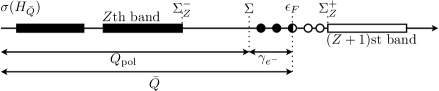
Figure 1. Decomposition $\bar{Q}=Q_{\rm pol}+\gamma_{e^{-}}$ for not too strong a positively charged nuclear defect ($\nu\geq 0$).

For a fixed external density $\nu$ and an adequately chosen chemical potential $\epsilon_{F}$, one can have ${\rm Tr}_{0}(\bar{Q})\neq 0$ meaning either that electron-hole pairs have been created from the Fermi sea, and/or that the system of lowest energy contains a finite number of bound electrons or holes close to the defect. In the applications, one will usually have for a positively charged nuclear defect ($\nu\geq 0$) that the spectrum of $H_{\bar{Q}}$ contains a sequence of eigenvalues converging to the bottom $\Sigma_{Z+1}^{-}$ of the lowest unfilled band (conduction band), and that $\epsilon_{F}$ is chosen such that exactly $q$ eigenvalues are filled, corresponding to $q$ bound electrons:

(3.13) $$\bar{Q}=\left(\chi_{(-\infty,\Sigma)}(H_{\bar{Q}})-\gamma^{0}_{\rm per}\right)+\left(\chi_{[\Sigma,\epsilon_{F})}(H_{\bar{Q}})+\delta\right):=Q_{\rm pol}+\gamma_{\rm e^{-}},$$

where we have chosen as a reference the center of the gap

$$\Sigma:=\frac{\Sigma^{+}_{Z}+\Sigma^{-}_{Z+1}}{2}.$$

For not too strong a defect density $\nu$, one has $\ker(H_{\bar{Q}}-\Sigma)=\{0\}$ and ${\rm Tr}_{0}(Q_{\rm pol})=0$. Hence ${\rm Tr}(\gamma_{\rm e^{-}})=q$. Let us assume for simplicity that $\delta=0$ and that $q\in{\mathbb{N}}\setminus\{0\}$. Then

(3.14) $$\gamma_{\rm e^{-}}=\chi_{[\Sigma,\epsilon_{F})}(H_{\bar{Q}})=\sum_{n=1}^{q}|\varphi_{n}\rangle\langle\varphi_{n}|$$

where $(\varphi_{n})$ are eigenfunctions of $H_{\bar{Q}}$ corresponding to its $q$ first eigenvalues in $[\Sigma,\epsilon_{F})$:

(3.15) $$H_{\bar{Q}}\varphi_{n}=\lambda_{n}\varphi_{n}.$$

Notice that

(3.16) $$H_{\bar{Q}}=-\Delta/2+(\rho_{\gamma_{\rm e^{-}}}-\nu)\ast|\cdot|^{-1}+V_{\rm pol}$$

where

$$V_{\rm pol}=(\rho_{\gamma^{0}_{\rm per}}-\mu_{\rm per})\star_{\Gamma}G_{1}+\rho_{Q_{\rm pol}}\ast|\cdot|^{-1}$$

is the polarization potential created by the self-consistent Fermi sea and seen by the $q$ electrons. Thus the $q$ electrons solve a usual reduced Hartree-Fock equation (3.15) in which the mean-field operator (3.16) additionally contains the self-consistent polarization of the medium.

The interpretation given in the previous paragraph is different if the positive density of charge $\nu$ of the defect is strong enough to create an electron-hole pair from the Fermi sea.

We end this section by specifying the regularity of solutions of (3.12). The proof is given in Section 5.4.

Proposition 2.

Let $\nu\in L^{1}({\mathbb{R}}^{3})\cap L^{2}({\mathbb{R}}^{3})$, $Z\in{\mathbb{N}}\setminus\left\{0\right\}$ and assume that (A1) holds. Any $Q\in\mathcal{K}$ solution of the self-consistent equation (3.12) belongs to $\mathcal{K}_{\rm r}$.

Remark 3.

Notice that it is natural to wonder whether $Q\in\mathfrak{S}_{1}$, which would in particular imply that $\rho_{Q}\in L^{1}({\mathbb{R}}^{3})$. This is known to be false for the Bogoliubov-Dirac-Fock model studied in [10, 11, 12, 13]. We do not answer this question for our model in the present paper.

3.3. Existence of minimizers under a charge constraint

In the previous section, we stated the existence of minimizers for any chemical potential in the gap of the periodic operator $H^{0}_{\rm per}$, but of course the total charge ${\rm Tr}_{0}(\bar{Q})$ of the obtained solution was unknown a priori. Here we tackle the more subtle problem of minimizing the energy while imposing a charge constraint. Mathematically this is more difficult because although the energy $\mathcal{E}^{\nu}(Q)$ is convex on $\mathcal{K}$ and weakly lower semi-continuous (wlsc) for the weak-$\ast$ topology of $\mathcal{Q}$ (as will be shown in the proof of Theorem 2), the $\gamma^{0}_{\rm per}$-trace functional $Q\in\mathcal{K}\mapsto{\rm Tr}_{0}(Q)$ is continuous but not wlsc for the weak-$\ast$ topology of $\mathcal{Q}$: in principle it is possible that a (positive or negative) part of the charge of a minimizing sequence for the charge-constrained minimization problem escapes to infinity, leaving at the limit a state of a different (lower or higher) charge. In fact, we can prove that a minimizer exists under a charge constraint, if and only if some binding conditions hold, the role of which being to prevent the lack of compactness.

As explained above, imposing ${\rm Tr}_{0}(Q)=q$ should intuitively lead (for a sufficiently weak defect density $\nu$) to a system of $q$ electrons coupled to a polarized Fermi sea. Notice that we do not impose that $q=\int_{{\mathbb{R}}^{3}}\nu$, i.e. our model allows a priori to treat defects with non-zero total charge.

As usual in reduced Hartree-Fock theories, we consider the case of a real charge constraint $q\in{\mathbb{R}}$:

(3.17) $$E^{\nu}(q):=\inf\{\mathcal{E}^{\nu}(Q),\ Q\in\mathcal{K},\ {\rm Tr}_{0}(Q)=q\}.$$

When no defect is present, $E^{0}(q)$ can be computed explicitly:

Proposition 3 (Defect-free charge-constrained energy).

Let $Z\in{\mathbb{N}}\setminus\left\{0\right\}$ and assume that (A1) holds. Then one has

$$E^{0}(q)=\left\{\begin{array}[]{ll}\Sigma^{-}_{Z+1}q&{\rm when\ }q\geq 0\\ \Sigma^{+}_{Z}q&{\rm when\ }q\leq 0.\\ \end{array}\right.$$

The minimization problem (3.17) with $\nu\equiv 0$ has no solution except when $q=0$.

The proof of Proposition 3 is given in Section 5.6. We now state the main result of this section, which is directly inspired from [12]:

Theorem 3 (Existence of minimizers under a charge constraint).

Let $\nu\in L^{1}({\mathbb{R}}^{3})\cap L^{2}({\mathbb{R}}^{3})$, $Z\in{\mathbb{N}}\setminus\left\{0\right\}$ and assume that (A1) holds. The following assertions are equivalent:

(a) Problem (3.17) admits a minimizer $\bar{Q}$;

(b) Every minimizing sequence for (3.17) is precompact in $\mathcal{Q}$ and converges towards a minimizer $\bar{Q}$ of (3.17);

(c) $\forall q^{\prime}\in{\mathbb{R}}\setminus\{0\},\quad E^{\nu}(q)<E^{\nu}(q-q^{\prime})+E^{0}(q^{\prime})$.

Assume that the equivalent conditions (a), (b) and (c) above are fulfilled. In this case, the minimizer $\bar{Q}$ is not necessarily unique, but all the minimizers share the same density $\bar{\rho}=\rho_{\bar{Q}}$. Besides, there exists $\epsilon_{F}\in[\Sigma^{+}_{Z},\Sigma^{-}_{Z+1}]$ such that the obtained minimizer $\bar{Q}$ is a global minimizer for $E^{\nu}_{\epsilon_{F}}$ defined in (3.11). It solves Equation (3.12) for some $0\leq\delta\leq 1$ with ${\rm Ran}(\delta)\subseteq\ker(H_{\bar{Q}}-\epsilon_{F})$. The operator $\delta$ is finite rank if $\epsilon_{F}\in(\Sigma^{+}_{Z},\Sigma^{-}_{Z+1})$ and trace-class if $\epsilon_{F}\in\{\Sigma^{+}_{Z},\Sigma^{-}_{Z+1}\}$.

Additionally the set of $q$’s in ${\mathbb{R}}$ satisfying the above equivalent conditions is a non-empty closed interval $I\subseteq{\mathbb{R}}$. This is the largest interval on which $q\mapsto E^{\nu}(q)$ is strictly convex.

Remark 4.

One has $I=\left\{{\rm Tr}_{0}(\bar{Q}),\ \bar{Q}\text{ min. of }E^{\nu}_{\epsilon_{F}},\ \epsilon_{F}\in[\Sigma_{Z}^{+},\Sigma_{Z+1}^{-}]\right\}$. Hence $I\neq\emptyset$ by Theorem 2.

Theorem 3 is proved in Section 5.8. Many of the above statements are very common in reduced Hartree-Fock theories and not all the details will be given (see, e.g. [31]). The difficult part is the proof that (b) is equivalent to (c), for which we use ideas from [12].

Conditions like (c) appear classically when analyzing the compactness properties of minimizing sequences, for instance by using the concentration-compactness principle of P.-L. Lions [24]. They are also very classical for linear models in which the bottom of the essential spectrum has the form of the minimum with respect to $q^{\prime}$ of the right hand side of (c), as expressed by the HVZ Theorem [16, 35, 36]. Assume for simplicity that $q>0$ and that $\bar{Q}$ can be written as in (3.13) and (3.14). When $0<q^{\prime}\leq q$, (c) means that it is not favorable to let $q^{\prime}$ electrons escape to infinity, while keeping $q-q^{\prime}$ electrons near the defect. When $q^{\prime}<0$, it means that it is not favorable to let $|q^{\prime}|$ holes escape to infinity, while keeping $q+|q^{\prime}|$ electrons near the defect. When $q^{\prime}>q$, it means that it is not favorable to let $q^{\prime}$ electrons escape to infinity, while keeping $q^{\prime}-q$ holes near the defect.

In this article we do not show when (c) holds true. Proving (c) usually requires some decay property of the density of charge $\rho_{\bar{Q}}$ for a solution $\bar{Q}$ of the nonlinear equation (3.12). In particular, knowing that $\rho_{\bar{Q}}\in L^{1}({\mathbb{R}}^{3})$ would be very useful (see Remark 3). We plan to investigate more closely the decay properties of $\rho_{\bar{Q}}$ and the validity of (c) in the near future. At present, the validity of a condition similar to (c) for the Bogoliubov-Dirac-Fock model was only proved in the nonrelativistic limit or in the weak coupling limit, see [12].

4. Thermodynamic limit of the supercell model

As mentioned before, we shall now justify the model of the previous section by proving that it is the thermodynamic limit of the supercell model.

Let us emphasize that there are several ways of performing thermodynamic limits. In [5], the authors consider a box of size $L$, $\Lambda_{L}:=[-L/2,L/2)^{3}$, and assume that the nuclei are located on ${\mathbb{Z}}^{3}\cap\Lambda_{L}$. Then they consider the rHF model of Section 1 for $N$ electrons living in the whole space, with $N=ZL^{3}$ chosen to impose neutrality. Denoting by $\rho_{L}$ the ground state electronic density of the latter problem, it is proved in [5, Thm 2.2] that the energy per unit cell converges to $I^{0}_{\rm per}$, and that the following holds:

(4.1) $$\sqrt{L^{-3}\sum_{k\in{\mathbb{Z}}^{3}\cap\Lambda_{L}}\rho_{{L}}(x-k)}\rightarrow\sqrt{\rho_{\gamma^{0}_{\rm per}}}$$

weakly in $H^{1}_{\rm loc}({\mathbb{R}}^{3})$, strongly in $L^{p}_{\rm loc}({\mathbb{R}}^{3})$ for all $2\leq p<6$ and almost everywhere on ${\mathbb{R}}^{3}$ when $L\to\infty$. Let us recall that $I^{0}_{\rm per}$ and $\gamma^{0}_{\rm per}$ are defined in Section 2.

Another way for performing thermodynamic limits is to confine the nuclei and the electrons in a domain $\Omega_{L}$ with $|\Omega_{L}|\to\infty$, by means of Dirichlet boundary conditions for the electrons. The latter approach was chosen for the Schrödinger model with quantum nuclei in the canonical and grand canonical ensembles [28] by Lieb and Lebowitz in the seminal paper [19] (see also [18]), where the existence of a limit for the energy per unit volume is proved. The crystal case in the Schrödinger model was tackled by Fefferman [9] in the same spirit. We do not know whether Fefferman’s proof can be adapted to treat the Hartree-Fock case.

Another possibility, perhaps less satisfactory from a physical viewpoint but more directly related to practical calculations (see e.g. [8]), is to take $\Omega_{L}=\Lambda_{L}$ and to impose periodic boundary conditions on the box $\Lambda_{L}$. Usually the Coulomb interaction is also replaced by a $(L{\mathbb{Z}}^{3})$-periodic Coulomb potential, leading to the so-called supercell model which will be described in detail below. This approach has the advantage of respecting the symmetry of the system in the crystal case. It was used by Hainzl, Lewin and Solovej in [13] to justify the Hartree-Fock approximation of no-photon Quantum Electrodynamics. The supercell limit of a linear model for photonic crystals is studied in [32].

Of course the conjecture is that the final results (the energy per unit cell and the ground state density of the crystal) should not depend on the chosen thermodynamic limit procedure. This is actually the case for the reduced Hartree-Fock model of the crystal. See [15] for a result in this direction for a model with quantum nuclei.

Let us now describe the supercell model. For $L\in{\mathbb{N}}\setminus\left\{0\right\}$, we introduce the supercell $\Lambda_{L}=[-L/2,L/2)^{3}$ and the Hilbert space

$$L^{2}_{\rm per}(\Lambda_{L})=\left\{\varphi\in L^{2}_{\rm loc}({\mathbb{R}}^{3})\ |\ \varphi\mbox{ $(L{\mathbb{Z}}^{3})$-periodic}\right\}.$$

We also introduce the $L{\mathbb{Z}}^{3}$-periodic Coulomb potential $G_{L}$ defined as the unique solution to

$$\left\{\begin{array}[]{l}\displaystyle-\Delta G_{L}=4\pi\left(\sum_{k\in L\,{\mathbb{Z}}^{3}}\delta_{k}-\frac{1}{L^{3}}\right)\\ G_{L}\ L\,{\mathbb{Z}}^{3}\mbox{-periodic},\ \ \mathop{\mbox{min}}_{{\mathbb{R}}^{3}}G_{L}=0.\end{array}\right.$$

It is easy to check that $G_{L}(x)=L^{-1}G_{1}(x/L)$ and that

$$G_{L}(x)=\frac{c}{L}+\sum_{k\in\frac{2\pi}{L}{\mathbb{Z}}^{3}\setminus\left\{0\right\}}\frac{4\pi}{|k|^{2}}\,\frac{1}{L^{3}}\,e^{ik\cdot x}.$$

For any $L{\mathbb{Z}}^{3}$-periodic function $g$, we define

$$\left(g\star_{\Lambda_{L}}G_{L}\right)(x):=\int_{\Lambda_{L}}G_{L}(x-y)\,g(y)\,dy,$$

$$D_{G_{L}}(f,g):=\int_{\Lambda_{L}}\int_{\Lambda_{L}}G_{L}(x-y)\,f(x)\,g(y)\,dx\,dy.$$

An admissible electronic state is then described by a one-body density matrix $\gamma$ in

$$\mathcal{P}_{{\rm sc},L}=\bigg{\{}\gamma\in\mathfrak{S}_{1}(L^{2}_{\rm per}(\Lambda_{L}))\ |\ \gamma^{\ast}=\gamma,\ 0\leq\gamma\leq 1,\ {\rm Tr}_{L^{2}_{\rm per}(\Lambda_{L})}(-\Delta\gamma)<+\infty\bigg{\}}.$$

Any $\gamma\in\mathcal{P}_{{\rm sc},L}$ has a well-defined density of charge $\rho_{\gamma}(x)=\gamma(x,x)$ where $\gamma(x,y)$ is the kernel of the operator $\gamma$. Notice that $\gamma(x+Lz,y+Lz^{\prime})=\gamma(x,y)$ for any $z,z^{\prime}\in{\mathbb{Z}}^{3}$, which implies that $\rho_{\gamma}$ is $L{\mathbb{Z}}^{3}$-periodic.

Throughout this section, we use the subscript ‘sc’ to indicate that we consider the thermodynamic limit of the supercell model.

4.1. Thermodynamic limit without defect

Because our model with defect uses the defect-free density matrix of the Fermi sea as a reference, we need to start with the study of the thermodynamic limit without defect. We are going to prove for the supercell model a result analogous to [5, Thm 2.2].

The reduced Hartree-Fock energy functional of the supercell model is defined for $\gamma\in\mathcal{P}_{{\rm sc},L}$ as

$$\framebox{$\displaystyle\mathcal{E}^{0}_{{\rm sc},L}(\gamma)={\rm Tr}_{L^{2}_{\rm per}(\Lambda_{L})}\left(-\frac{1}{2}\Delta\gamma\right)+\frac{1}{2}D_{G_{L}}\left(\rho_{\gamma}-\mu_{\rm per},\rho_{\gamma}-\mu_{\rm per}\right)$}$$

where we recall that $\mu_{\rm per}(x)=\sum_{R\in{\mathbb{Z}}^{3}}Zm(x-R)$ is a ${\mathbb{Z}}^{3}$- (thus $L{\mathbb{Z}}^{3}$-) periodic function. The reduced Hartree-Fock ground state energy for a neutral system in the box of size $L$ is then given by

(4.2) $$\framebox{$\displaystyle I^{0}_{{\rm sc},L}=\inf\left\{\mathcal{E}^{0}_{{\rm sc},L}(\gamma),\;\gamma\in\mathcal{P}_{{\rm sc},L},\ \int_{\Lambda_{L}}\rho_{\gamma}=\int_{\Lambda_{L}}\mu_{\rm per}=ZL^{3}\right\}.$}$$

Let us recall that $I^{0}_{\rm per}$, $\gamma^{0}_{\rm per}$ and $H^{0}_{\rm per}$ are defined in Section 2. In Section 5.9, we prove the following

Theorem 4 (Thermodynamic limit of the defect-free supercell model).

Let $Z>0$.

i) For all $L\in{\mathbb{N}}\setminus\{0\}$, the minimizing problem $I^{0}_{{\rm sc},L}$ has at least one minimizer, and all the minimizers share the same density. This density is ${\mathbb{Z}}^{3}$-periodic. Besides, there is one minimizer $\gamma^{0}_{{\rm sc},L}$ of (4.2) which commutes with the translations $\tau_{k}$, $k\in{\mathbb{Z}}^{3}$.

ii) The following thermodynamic limit properties hold true:

$\bullet$ (Convergence of the energy per unit cell).

$$\lim_{L\to\infty}\frac{I^{0}_{{\rm sc},L}}{L^{3}}=I^{0}_{\rm per};$$

$\bullet$ (Convergence of the density).

(4.3) $$\sqrt{\rho_{\gamma^{0}_{{\rm sc},L}}}\rightharpoonup\sqrt{\rho_{\gamma^{0}_{\rm per}}}\quad\text{weakly in}\ H^{1}_{\rm loc}({\mathbb{R}}^{3}),$$

$${\rho_{\gamma^{0}_{{\rm sc},L}}}\to{\rho_{\gamma^{0}_{\rm per}}}\quad\text{strongly in\ }L^{p}_{\rm loc}({\mathbb{R}}^{3})\ \text{ for}\ 1\leq p<3\text{\ and a.e.};$$

$\bullet$ (Convergence of the mean-field Hamiltonian and its spectrum). Let

$$H^{0}_{{\rm sc},L}=-\frac{\Delta}{2}+(\rho_{\gamma^{0}_{{\rm sc},L}}-\mu_{\rm per})\star_{\Gamma}G_{1}$$

seen as an operator acting on $L^{2}({\mathbb{R}}^{3})$. Then, for all $L\in{\mathbb{N}}\setminus\{0\}$, $H^{0}_{{\rm sc},L}-H^{0}_{\rm per}$ is a bounded operator and

$$\lim_{L\to\infty}\left|\!\left|H^{0}_{{\rm sc},L}-H^{0}_{\rm per}\right|\!\right|=0.$$

Denoting by $(\lambda_{n}^{L}(\xi))_{n\in{\mathbb{N}}\setminus\{0\}}$ the nondecreasing sequence of eigenvalues of $(H^{0}_{{\rm sc},L})_{\xi}$ for $\xi\in\Gamma^{\ast}$, one has

(4.4) $$\lim_{L\to\infty}\sup_{n\in{\mathbb{N}}\setminus\left\{0\right\}}\sup_{\xi\in\Gamma^{\ast}}\left|\lambda_{n}^{L}(\xi)-\lambda_{n}(\xi)\right|=0$$

where $(\lambda_{n}(\xi))_{n\geq 1}$ are the eigenvalues of $(H^{0}_{\rm per})_{\xi}$ introduced in Theorem 1.

iii) Assume in addition that (A1) holds. Fix some $\epsilon_{F}\in(\Sigma^{+}_{Z},\Sigma^{-}_{Z+1})$. Then for $L$ large enough, the minimizer $\gamma^{0}_{{\rm sc},L}$ of $I^{0}_{{\rm sc},L}$ is unique. It is also the unique minimizer of the following problem

(4.5) $$I^{0}_{{\rm sc},L,\epsilon_{F}}:=\inf\left\{\mathcal{E}^{0}_{{\rm sc},L}(\gamma)-\epsilon_{F}{\rm Tr}_{L^{2}_{\rm per}(\Lambda_{L})}(\gamma),\quad\gamma\in\mathcal{P}_{{\rm sc},L}\right\}.$$

Remark 5.

Notice that some of the above assertions are more precise for the supercell model than for the thermodynamic limit procedure considered in [5, Thm 2.2] (compare for instance (4.3) with (4.1)). This is because the supercell model respects the symmetry of the system, allowing in particular to have a minimizer $\gamma^{0}_{{\rm sc},L}$ in the box of size $L^{3}$ which is periodic for the lattice ${\mathbb{Z}}^{3}$. For an insulator, the uniqueness of $\gamma^{0}_{{\rm sc},L}$ for large $L$ and the convergence properties of iii) are also very interesting for computational purposes.

4.2. Thermodynamic limit with defect

We end this section by considering the thermodynamic limit of the supercell model with a defect. Recall that $\nu\in L^{1}({\mathbb{R}}^{3})\cap L^{2}({\mathbb{R}}^{3})\subset\mathcal{C}$ is the density of charge of the defect. First we need to periodize this function with respect to the large box $\Lambda_{L}$, for instance by defining

$$\nu_{L}(x):=\sum_{z\in{\mathbb{Z}}^{3}}({\mathds{1}}_{\Lambda_{L}}\nu)(\cdot-Lz).$$

The reduced Hartree-Fock energy functional of the supercell model with defect is then defined for $\gamma\in\mathcal{P}_{{\rm sc},L}$ as

$$\framebox{$\displaystyle\mathcal{E}^{\nu}_{{\rm sc},L}(\gamma)={\rm Tr}_{L^{2}_{\rm per}(\Lambda_{L})}\left(-\frac{1}{2}\Delta\gamma\right)+\frac{1}{2}D_{G_{L}}\left(\rho_{\gamma}-\mu_{\rm per}-\nu_{L},\rho_{\gamma}-\mu_{\rm per}-\nu_{L}\right).$}$$

For $\epsilon_{F}\in(\Sigma^{+}_{Z},\Sigma^{-}_{Z+1})$, we consider the following minimization problem

(4.6) $$\framebox{$\displaystyle I^{\nu}_{{\rm sc},L,\epsilon_{F}}=\inf\left\{\mathcal{E}^{\nu}_{{\rm sc},L}(\gamma)-\epsilon_{F}{\rm Tr}_{L^{2}_{\rm per}(\Lambda_{L})}(\gamma),\;\gamma\in\mathcal{P}_{{\rm sc},L}\right\}.$}$$

We recall that $\gamma^{0}_{\rm per}$ is defined in Section 2, that $E_{\kappa}^{\nu}$ and $\bar{Q}$ are defined in Section 3.2, and that $I^{0}_{{\rm sc},L,\epsilon_{F}}$ is defined in Section 4.1. In Section 5.10, we prove the

Theorem 5 (Thermodynamic limit of the supercell model with defect).

Let $Z\in{\mathbb{N}}\setminus\left\{0\right\}$. Assume that (A1) holds and fix some $\epsilon_{F}\in(\Sigma^{+}_{Z},\Sigma^{-}_{Z+1})$. Then one has

(4.7) $$\lim_{L\to\infty}\left(I^{\nu}_{{\rm sc},L,\epsilon_{F}}-I^{0}_{{\rm sc},L,\epsilon_{F}}\right)=E_{\epsilon_{F}}^{\nu}-\int_{{\mathbb{R}}^{3}}\nu\left((\rho_{\gamma^{0}_{\rm per}}-\mu_{\rm per})\star_{\Gamma}G_{1}\right)+\frac{1}{2}D(\nu,\nu).$$

Additionally, if $\gamma_{{\rm sc},L}^{\nu}$ denotes a minimizer for (4.6), then one has, up to extraction of a subsequence,

$$(\gamma^{\nu}_{{\rm sc},L}-\gamma^{0}_{{\rm sc},L})(x,y)\to\bar{Q}(x,y)$$

weakly in $H^{1}_{\rm loc}({\mathbb{R}}^{3}\times{\mathbb{R}}^{3})$ and strongly in $L^{2}_{\rm loc}({\mathbb{R}}^{3}\times{\mathbb{R}}^{3})$, where $\bar{Q}$ is a minimizer of (3.11), as obtained in Theorem 2. Besides,

$$\rho_{\gamma^{\nu}_{{\rm sc},L}}-\rho_{\gamma^{0}_{{\rm sc},L}}\to\bar{\rho}$$

weakly in $L^{2}_{\rm loc}({\mathbb{R}}^{3})$, where $\bar{\rho}$ is the common density of all the minimizers of (3.11).

Remark 6.

In numerical simulations, the right-hand side of (4.7) is approximated by $I^{\nu}_{{\rm sc},L,\epsilon_{F}}-I^{0}_{{\rm sc},L,\epsilon_{F}}$ for a given value of $L$. This approach has several drawbacks. First, the values of $L$ that lead to tractable numerical simulations are in many cases much too small to obtain a correct estimation of the limit $L\to\infty$. Second, it is not easy to extend this method for computing $E^{\nu}_{\epsilon_{F}}$, to the direct evaluation of $E^{\nu}(q)$ for a given $q$ (i.e. the energy of a defect with a prescribed total charge). The formalism introduced in the present article (problems (3.11) and (3.17)) suggests an alternative way for computing energies of defects in crystalline materials. A work in this direction was already started [3].

5. Proof of the main results

Unless otherwise stated, the operators used in the following proofs are considered as operators on $L^{2}({\mathbb{R}}^{3})$.

5.1. Useful estimates

We gather in this section some results which we shall need throughout the proofs. We start with the

5.1.1. Proof of Lemma 1

Recall that $H^{0}_{\rm per}=-\Delta/2+V_{\rm per}$ with $V_{\rm per}:=(\rho_{\gamma^{0}_{\rm per}}-\mu_{\rm per})\star_{\Gamma}G_{1}\in L^{\infty}({\mathbb{R}}^{3})$. Thus $|H^{0}_{\rm per}-\kappa|\geq H^{0}_{\rm per}-\kappa\geq-\Delta/2-C$ for some large enough constant $C$. On the other hand, as $\kappa\in(\Sigma_{Z}^{+},\Sigma_{Z+1}^{-})$, there exists $\alpha>0$ such that $\left|H^{0}_{\rm per}-\kappa\right|\geq\alpha$. This implies that

$$|H^{0}_{\rm per}-\kappa|\geq\max(-\Delta/2-C,\alpha)\geq c_{1}(1-\Delta)$$

for some constant $c_{1}>0$. The proof of the upper bound in (3.7) is straightforward.

Then $(-\Delta/2+c)^{-1}(H^{0}_{\rm per}-\kappa+c)=1+(-\Delta/2+c)^{-1}(V_{\rm per}-\kappa)$ is a bounded invertible operator for $c$ large enough, since

$$\left|\!\left|(-\Delta/2+c)^{-1}(V_{\rm per}-\kappa)\right|\!\right|\leq\frac{\left|\!\left|V_{\rm per}\right|\!\right|_{L^{\infty}}+|\kappa|}{c}.$$

Thus $(H^{0}_{\rm per}-\kappa+c)^{-1}(-\Delta/2+c)$ is bounded for a well-chosen $c\gg 1$, which clearly implies that

$$(H^{0}_{\rm per}-\kappa)^{-1}(-\Delta+1)=\frac{H^{0}_{\rm per}-\kappa+c}{H^{0}_{\rm per}-\kappa}(H^{0}_{\rm per}-\kappa+c)^{-1}(-\Delta/2+c)\frac{-\Delta+1}{-\Delta/2+c}$$

is also bounded, together with its inverse.∎

5.1.2. Some commutator estimates

Throughout this paper, we shall use Cauchy’s formula to express the projector ${\gamma^{0}_{\rm per}}$:

(5.1) $${\gamma^{0}_{\rm per}}=\frac{1}{2i\pi}\int_{\mathscr{C}}(z-H^{0}_{\rm per})^{-1}\,dz,$$

where $\mathscr{C}$ is a fixed regular bounded closed contour enclosing the lowest $Z$ bands of the spectrum of $H^{0}_{\rm per}$.

The following result will be a useful tool to replace the resolvent $(z-H^{0}_{\rm per})^{-1}$ with the operator $(-\Delta+1)^{-1}$ which will be easier to manipulate. Its proof is the same as the one of Lemma 1.

Lemma 3.

The operator $B(z):=(z-H^{0}_{\rm per})^{-1}(-\Delta+1)$ and its inverse are bounded uniformly in $z\in\mathscr{C}$.

The next result provides some useful properties of commutators:

Lemma 4.

The operators $[\gamma^{0}_{\rm per},\Delta]$ and $(1-\Delta)\,[\gamma^{0}_{\rm per},|\nabla|]\,(1-\Delta)$ are bounded.

Proof.

The boundedness of $[\gamma^{0}_{\rm per},\Delta]$ follows from (5.1) and from the fact that $[(z-H^{0}_{\rm per})^{-1},\Delta]$ is bounded uniformly in $z\in\mathscr{C}$ by Lemma 3.

Using again (5.1), it suffices to prove that $(1-\Delta)[(z-H^{0}_{\rm per})^{-1},|\nabla|](1-\Delta)$ is bounded uniformly in $z\in\mathscr{C}$ to infer that $(1-\Delta)\,[\gamma^{0}_{\rm per},|\nabla|]\,(1-\Delta)$ is bounded. In order to prove the uniform boundedness of $(1-\Delta)[(z-H^{0}_{\rm per})^{-1},|\nabla|](1-\Delta)$, we use the formal equality

(5.2) $$[(z-A)^{-1},B]=(z-A)^{-1}[A,B](z-A)^{-1}.$$

We thus obtain

(5.3) $$(1-\Delta)[(z-H^{0}_{\rm per})^{-1},|\nabla|](1-\Delta)=B(z)^{*}\left[|\nabla|,V_{\rm per}\right]B(z).$$

Using (5.1) and lemma 3, we obtain

$$\|(1-\Delta)[{\gamma^{0}_{\rm per}},|\nabla|](1-\Delta)\|\leq C\left|\!\left|\left[|\nabla|,V_{\rm per}\right]\right|\!\right|\leq C\left|\!\left|\nabla V_{\rm per}\right|\!\right|_{L^{\infty}({\mathbb{R}}^{3})}.$$

∎

Lemma 5.

Let $V=V_{1}+V_{2}$ with $V_{1}\in\mathcal{C}^{\prime}$ and $V_{2}\in L^{2}({\mathbb{R}}^{3})$. Then $[{\gamma^{0}_{\rm per}},V]\in\mathfrak{S}_{2}$ and there exists a positive real constant $C$ such that

$$\|[{\gamma^{0}_{\rm per}},V]\|_{\mathfrak{S}_{2}}\leq C(\|V_{1}\|_{\mathcal{C}^{\prime}}+\left|\!\left|V_{2}\right|\!\right|_{L^{2}({\mathbb{R}}^{3})}).$$

Proof.

Formulas (5.1) and (5.2) lead to

$$[{\gamma^{0}_{\rm per}},V_{2}] = -\frac{1}{4i\pi}\int_{\mathscr{C}}B(z)(-\Delta+1)^{-1}[\Delta,V_{2}](-\Delta+1)^{-1}B(z)^{*}\,dz$$

$$= -\frac{1}{4i\pi}\int_{\mathscr{C}}B(z)((-\Delta+1)^{-1}\Delta)V_{2}(-\Delta+1)^{-1}B(z)^{*}\,dz$$

$$\qquad\qquad\qquad+\frac{1}{4i\pi}\int_{\mathscr{C}}B(z)(-\Delta+1)^{-1}V_{2}(\Delta(-\Delta+1)^{-1})B(z)^{*}\,dz.$$

As $(-\Delta+1)^{-1}$ and $(-\Delta+1)^{-1}\Delta$ are bounded operators, we obtain, using Lemma 3,

$$\left|\!\left|[{\gamma^{0}_{\rm per}},V_{2}]\right|\!\right|_{\mathfrak{S}_{2}}\leq C\left|\!\left|(-\Delta+1)^{-1}V_{2}\right|\!\right|_{\mathfrak{S}_{2}},$$

for some constant $C$ independent of $V_{2}$. Likewise,

$$[{\gamma^{0}_{\rm per}},V_{1}] = -\frac{1}{4i\pi}\int_{\mathscr{C}}B(z)(-\Delta+1)^{-1}[\Delta,V_{1}](-\Delta+1)^{-1}B(z)^{*}\,dz$$

$$= -\sum_{i=1}^{3}\frac{1}{4i\pi}\int_{\mathscr{C}}B(z)\left((-\Delta+1)^{-1}\partial_{x_{i}}\right)\frac{\partial V_{1}}{\partial{x_{i}}}(-\Delta+1)^{-1}B(z)^{*}\,dz$$

$$\qquad+\sum_{i=1}^{3}\frac{1}{4i\pi}\int_{\mathscr{C}}B(z)(-\Delta+1)^{-1}\frac{\partial V_{1}}{\partial{x_{i}}}\left(\partial_{x_{i}}(-\Delta+1)^{-1}\right))B(z)^{*}\,dz,$$

which implies

$$\left|\!\left|[{\gamma^{0}_{\rm per}},V_{1}]\right|\!\right|_{\mathfrak{S}_{2}}\leq C\left|\!\left|(-\Delta+1)^{-1}\nabla V_{1}\right|\!\right|_{\mathfrak{S}_{2}}$$

for some constant $C$ independent of $V_{1}$. We then use the Kato-Seiler-Simon inequality (see [29] and [30, Thm 4.1])

(5.4) $$\forall p\geq 2,\qquad\left|\!\left|f(-i\nabla)g(x)\right|\!\right|_{\mathfrak{S}_{p}}\leq(2\pi)^{-3/p}\left|\!\left|g\right|\!\right|_{L^{p}({\mathbb{R}}^{3})}\left|\!\left|f\right|\!\right|_{L^{p}({\mathbb{R}}^{3})}$$

to infer

(5.5) $$\left|\!\left|[{\gamma^{0}_{\rm per}},V_{2}]\right|\!\right|_{\mathfrak{S}_{2}}\leq C^{\prime}\left|\!\left|V_{2}\right|\!\right|_{L^{2}({\mathbb{R}}^{3})},$$

(5.6) $$\left|\!\left|[{\gamma^{0}_{\rm per}},V_{1}]\right|\!\right|_{\mathfrak{S}_{2}}\leq C^{\prime}\left|\!\left|\nabla V_{1}\right|\!\right|_{L^{2}({\mathbb{R}}^{3})}=C^{\prime}\left|\!\left|V_{1}\right|\!\right|_{\mathcal{C}^{\prime}}.$$

∎

Lemma 6.

The operator $[\,|H^{0}_{\rm per}-\kappa|,|\nabla|\,]$ is bounded for any $\kappa$ in the gap $(\Sigma^{+}_{Z},\Sigma^{-}_{Z+1})$.

Proof.

We have $|H^{0}_{\rm per}-\kappa|=-(H^{0}_{\rm per}-\kappa){\gamma^{0}_{\rm per}}+(H^{0}_{\rm per}-\kappa)(1-{\gamma^{0}_{\rm per}})$ and thus

$$[\,|H^{0}_{\rm per}-\kappa|,|\nabla|\,] = -2(H^{0}_{\rm per}-\kappa)[{\gamma^{0}_{\rm per}},|\nabla|]+[|\nabla|,V_{\rm per}](2{\gamma^{0}_{\rm per}}-1)$$

$$= 2(B(\kappa)^{*})^{-1}(1-\Delta)[{\gamma^{0}_{\rm per}},|\nabla|]+[|\nabla|,V_{\rm per}](2{\gamma^{0}_{\rm per}}-1)$$

which gives the result since $\left|\!\left|[|\nabla|,V_{\rm per}]\right|\!\right|\leq\left|\!\left|\nabla V_{\rm per}\right|\!\right|_{L^{\infty}({\mathbb{R}}^{3})}$ and $(1-\Delta)[{\gamma^{0}_{\rm per}},|\nabla|]$ is bounded by Lemma 4. ∎

5.2. Proof of Proposition 1

Let $V=V_{1}+V_{2}$ where $V_{1}\in\mathcal{C}^{\prime}$ and $V_{2}\in L^{2}({\mathbb{R}}^{3})\cap L^{\infty}({\mathbb{R}}^{3})$, and $Q\in\mathcal{Q}$. Notice that

$$(QV)^{++}=Q^{++}V(\gamma_{\rm per}^{0})^{\perp}+Q^{+-}[\gamma_{\rm per}^{0},V](\gamma_{\rm per}^{0})^{\perp},$$

(5.7) $$(QV)^{--}=Q^{--}V\gamma_{\rm per}^{0}-Q^{-+}[\gamma_{\rm per}^{0},V]\gamma_{\rm per}^{0},$$

where $(\gamma_{\rm per}^{0})^{\perp}=1-\gamma_{\rm per}^{0}$. We only treat the $(QV)^{--}$ term, the argument being the same for $(QV)^{++}$.

First we write $Q^{--}V\gamma_{\rm per}^{0}=Q^{--}(1+|\nabla|)(1+|\nabla|)^{-1}V\gamma^{0}_{\rm per}$ and notice that $(1+|\nabla|)^{-1}V$ is bounded since $V_{2}\in L^{\infty}({\mathbb{R}}^{3})$ by assumption and

$$\left|\!\left|(1+|\nabla|)^{-1}V_{1}\right|\!\right|_{\mathfrak{S}_{6}}\leq C\left|\!\left|V_{1}\right|\!\right|_{L^{6}}\leq C^{\prime}\left|\!\left|\nabla V_{1}\right|\!\right|_{L^{2}}=C^{\prime}\left|\!\left|V_{1}\right|\!\right|_{\mathcal{C}^{\prime}}$$

by the Kato-Seiler-Simon inequality (5.4) and the critical Sobolev embedding of $H^{1}({\mathbb{R}}^{3})$ in $L^{6}({\mathbb{R}}^{3})$. This proves that $Q^{--}V\gamma_{\rm per}^{0}$ is a trace-class operator. Thus the following is true:

$$|{\rm Tr}(Q^{--}V\gamma_{\rm per}^{0})| = |{\rm Tr}(Q^{--}V)|$$

$$= |{\rm Tr}((1+|\nabla|)Q^{--}(1+|\nabla|)(1+|\nabla|)^{-1}V(1+|\nabla|)^{-1})|$$

$$\leq \left|\!\left|Q\right|\!\right|_{\mathcal{Q}}\left|\!\left|(1+|\nabla|)^{-1}V(1+|\nabla|)^{-1}\right|\!\right|_{\mathfrak{S}_{\infty}}.$$

Then

$$\left|\!\left|(1+|\nabla|)^{-1}V_{1}(1+|\nabla|)^{-1}\right|\!\right|_{\mathfrak{S}_{\infty}} \leq \left|\!\left|(1+|\nabla|)^{-1}V_{1}\right|\!\right|_{\mathfrak{S}_{6}}\left|\!\left|(1+|\nabla|)^{-1}\right|\!\right|$$

$$\leq C\left|\!\left|V_{1}\right|\!\right|_{L^{6}}\leq C^{\prime}\left|\!\left|V_{1}\right|\!\right|_{\mathcal{C}^{\prime}},$$

and

$$\left|\!\left|(1+|\nabla|)^{-1}V_{2}(1+|\nabla|)^{-1}\right|\!\right|_{\mathfrak{S}_{\infty}} \leq \left|\!\left|(1+|\nabla|)^{-1}|V_{2}|(1+|\nabla|)^{-1}\right|\!\right|_{\mathfrak{S}_{\infty}}$$

$$\leq \left|\!\left|(1+|\nabla|)^{-1}|V_{2}|^{1/2}\right|\!\right|_{\mathfrak{S}_{4}}^{2}\leq C\left|\!\left|V_{2}\right|\!\right|_{L^{2}}.$$

Hence,

$$|{\rm Tr}(Q^{--}V\gamma_{\rm per}^{0})|\leq C\,\left|\!\left|Q\right|\!\right|_{\mathcal{Q}}(\left|\!\left|V_{1}\right|\!\right|_{\mathcal{C}^{\prime}}+\left|\!\left|V_{2}\right|\!\right|_{L^{2}}).$$

For the second term of (5.7), we just use Lemma 5 which tells us that $Q^{-+}[\gamma_{\rm per}^{0},V]\gamma_{\rm per}^{0}\in\mathfrak{S}_{1}$ since $Q^{-+}\in\mathfrak{S}_{2}$ and $[\gamma_{\rm per}^{0},V]\in\mathfrak{S}_{2}$. Additionally

$$|{\rm Tr}(Q^{-+}[\gamma_{\rm per}^{0},V]\gamma_{\rm per}^{0})|\leq\left|\!\left|Q^{-+}[\gamma_{\rm per}^{0},V]\gamma_{\rm per}^{0}\right|\!\right|_{\mathfrak{S}_{1}}\leq C\left|\!\left|Q^{-+}\right|\!\right|_{\mathfrak{S}_{2}}(\left|\!\left|V_{1}\right|\!\right|_{\mathcal{C}^{\prime}}+\left|\!\left|V_{2}\right|\!\right|_{L^{2}}).$$

The end of the proof of Proposition 1 is then obvious. ∎

5.3. Proof of Lemma 2

Let $Q\in\mathcal{Q}$. For $\epsilon>0$, we introduce the following regularization operator

(5.8) $$R_{\epsilon}:=(1+\epsilon|H^{0}_{\rm per}-\Sigma|)^{-1}$$

and set

$$Q_{\epsilon}:=R_{\epsilon}QR_{\epsilon}.$$

Notice first that $Q_{\epsilon}\in\mathcal{Q}_{\rm r}$. Indeed, using the same notation as in Lemma 3, we obtain

$$(1-\Delta)R_{\epsilon}=(1-\Delta)(H^{0}_{\rm per}-\Sigma)^{-1}\frac{H^{0}_{\rm per}-\Sigma}{1+\epsilon|H^{0}_{\rm per}-\Sigma|}=-B(\Sigma)^{*}\frac{H^{0}_{\rm per}-\Sigma}{1+\epsilon|H^{0}_{\rm per}-\Sigma|}$$

which shows that $\|(1-\Delta)R_{\epsilon}\|\leq\epsilon^{-1}\|B(\Sigma)^{*}\|.$ Similarly, $\|R_{\epsilon}(1-\Delta)\|\leq\epsilon^{-1}\|B(\Sigma)\|$. As $R_{\epsilon}$ commutes with $\gamma^{0}_{\rm per}$, we infer

$$(1-\Delta)Q_{\epsilon}^{--}(1-\Delta)=(1-\Delta)R_{\epsilon}Q^{--}R_{\epsilon}(1-\Delta)\in\mathfrak{S}_{1}.$$

Likewise, $(1-\Delta)Q_{\epsilon}^{++}(1-\Delta)\in\mathfrak{S}_{1}$. Then we show that $Q_{\epsilon}\in\mathcal{K}_{\rm r}\subset\mathcal{K}$ when $Q\in\mathcal{K}$. To prove this, we use the fact that $-\gamma^{0}_{\rm per}\leq Q\leq 1-\gamma^{0}_{\rm per}$ is equivalent to $Q^{2}\leq Q^{++}-Q^{--}$ (see Section 3.1). As $\|R_{\epsilon}\|\leq 1$, we obtain

(5.9) $$(Q_{\epsilon})^{2}=R_{\epsilon}Q(R_{\epsilon})^{2}QR_{\epsilon}\leq R_{\epsilon}Q^{2}R_{\epsilon}\\ \leq R_{\epsilon}(Q^{++}-Q^{--})R_{\epsilon}=(Q_{\epsilon})^{++}-(Q_{\epsilon})^{--}$$

where we have used that $(R_{\epsilon})^{2}\leq 1$ and that $\gamma^{0}_{\rm per}$ commutes with $R_{\epsilon}$. Hence, it only remains to prove that $Q_{\epsilon}\to Q$ for the $\mathcal{Q}$-topology as $\epsilon\to 0$, for any fixed $Q\in\mathcal{Q}$. We shall need the

Lemma 7.

For any $1\leq p<\infty$ and any fixed $Q\in\mathfrak{S}_{p}$, one has

(5.10) $$\lim_{\epsilon\to 0}\left|\!\left|R_{\epsilon}Q-Q\right|\!\right|_{\mathfrak{S}_{p}}=0.$$

Proof.

Notice that

$$R_{\epsilon}-1=-\frac{\epsilon|H^{0}_{\rm per}-\Sigma|}{1+\epsilon|H^{0}_{\rm per}-\Sigma|}$$

satisfies $\|R_{\epsilon}-1\|\leq 1$. Hence $\left|\!\left|(R_{\epsilon}-1)Q\right|\!\right|_{\mathfrak{S}_{p}}\leq\left|\!\left|Q\right|\!\right|_{\mathfrak{S}_{p}}.$ By linearity and density of “smooth” finite rank operators in $\mathfrak{S}_{p}$ for any $1\leq p<\infty$, it suffices to prove (5.10) for $Q=|f\rangle\langle f|$ with $f\in H^{2}({\mathbb{R}}^{3})$. Then

$$\left|\!\left|(R_{\epsilon}-1)|f\rangle\langle f|\right|\!\right|_{\mathfrak{S}_{1}}\leq\left|\!\left|(R_{\epsilon}-1)f\right|\!\right|_{L^{2}}\left|\!\left|f\right|\!\right|_{L^{2}}\leq\epsilon\left|\!\left||H^{0}_{\rm per}-\Sigma|f\right|\!\right|_{L^{2}}\left|\!\left|f\right|\!\right|_{L^{2}}$$

which converges to 0 as $\epsilon\to 0$ and controls $\left|\!\left|(R_{\epsilon}-1)|f\rangle\langle f|\right|\!\right|_{\mathfrak{S}_{p}}$ for $1\leq p<\infty$. ∎

We are now able to complete the proof of Lemma 2. First, by (5.2)

$$[R_{\epsilon},|\nabla|]=-\epsilon R_{\epsilon}\;\left[|H^{0}_{\rm per}-\Sigma|,|\nabla|\right]\;R_{\epsilon}$$

and therefore by Lemma 6 there exists a constant $C>0$ such that

(5.11) $$\|\;[R_{\epsilon},|\nabla|]\;\|\leq C\epsilon.$$

Hence, $\lim_{\epsilon\to 0}\|\;[R_{\epsilon},|\nabla|]\;\|=0$. Compute now for instance

$$|\nabla|(R_{\epsilon}QR_{\epsilon}-Q)^{--}|\nabla| = |\nabla|((R_{\epsilon}-1)Q^{--}R_{\epsilon}+Q^{--}(R_{\epsilon}-1))|\nabla|$$

$$= [|\nabla|,R_{\epsilon}]Q^{--}[R_{\epsilon},|\nabla|]+[|\nabla|,R_{\epsilon}]Q^{--}|\nabla|R_{\epsilon}$$

$$\quad+(R_{\epsilon}-1)|\nabla|Q^{--}[R_{\epsilon},|\nabla|]+|\nabla|Q^{--}[R_{\epsilon},|\nabla|]$$

$$\quad+(R_{\epsilon}-1)|\nabla|Q^{--}|\nabla|R_{\epsilon}+|\nabla|Q^{--}|\nabla|(R_{\epsilon}-1).$$

Applying either (5.11) or Lemma 7 to each term of the previous expression allows to conclude that

$$\lim_{\epsilon\to 0}\left|\!\left||\nabla|(Q_{\epsilon}^{--}-Q^{--})|\nabla|\right|\!\right|_{\mathfrak{S}_{1}}=0.$$

The proof is the same for the other terms in the definition of $\left|\!\left|\cdot\right|\!\right|_{\mathcal{Q}}$. ∎

5.4. Proof of Proposition 2: regularity of solutions

Let $Q\in\mathcal{Q}$ be of the form

$$Q=\chi_{(-\infty,\epsilon_{F})}(H^{0}_{\rm per}+V)-{\gamma^{0}_{\rm per}}+\delta$$

where $0\leq\delta\leq 1$ is a finite rank operator with $\text{Ran}(\delta)\subseteq\ker(H^{0}_{\rm per}+V-\epsilon_{F})$ and $V=\rho\ast|\cdot|^{-1}$ for some $\rho\in L^{1}({\mathbb{R}}^{3})\cap L^{2}({\mathbb{R}}^{3})$ (in our case $\rho=\rho_{Q}-\nu$). Note that $V\in\mathcal{C}^{\prime}\cap L^{\infty}({\mathbb{R}}^{3})$ since

$$\left|\!\left|V\right|\!\right|_{L^{\infty}} \leq (2\pi)^{-3/2}\int_{{\mathbb{R}}^{3}}|\widehat{V}(k)|dk=C\int_{{\mathbb{R}}^{3}}\frac{|\widehat{\rho}(k)|}{|k|^{2}}dk$$

$$\leq C\left(\int_{{\mathbb{R}}^{3}}\frac{|\widehat{\rho}(k)|^{2}(1+|k|^{2})}{|k|^{2}}dk\right)^{1/2}\left(\int_{{\mathbb{R}}^{3}}\frac{dk}{|k|^{2}(1+|k|^{2})}\right)^{1/2}<\infty.$$

Since $\ker(H^{0}_{\rm per}+V-\epsilon_{F})\subseteq\mathcal{D}(H^{0}_{\rm per}+V)=\mathcal{D}(H^{0}_{\rm per})=H^{2}({\mathbb{R}}^{3})$, it is clear that the finite rank operator $\delta$ satisfies $(1-\Delta)\delta(1-\Delta)\in\mathfrak{S}_{1}$. Thus, up to a change of $\epsilon_{F}$, we can assume that $\ker(H^{0}_{\rm per}+V-\epsilon_{F})=\{0\}$ and that $\delta=0$:

$$Q=\chi_{(-\infty,\epsilon_{F})}(H^{0}_{\rm per}+V)-{\gamma^{0}_{\rm per}}.$$

Then we remark that $Q^{2}=Q^{++}-Q^{--}$, hence we only have to prove that $(1-\Delta)Q\in\mathfrak{S}_{2}$.

Let $\mathscr{C}$ be a smooth curve enclosing the whole spectrum of $H^{0}_{\rm per}+V$ below $\epsilon_{F}$. Since $V\in L^{\infty}({\mathbb{R}}^{3})$ and $|H^{0}_{\rm per}+V-z|\geq c>0$ uniformly in $z\in\mathscr{C}$, we can mimic the proof of Lemma 3 and find that

(5.12) $$\sup_{z\in\mathscr{C}}\|(1-\Delta)(H^{0}_{\rm per}+V-z)^{-1}\|<\infty.$$

We then use Cauchy’s formula (5.1) and iterate the resolvent formula

$$(z-H^{0}_{\rm per}-V)^{-1}=(z-H^{0}_{\rm per})^{-1}+(z-H^{0}_{\rm per}-V)^{-1}V(z-H^{0}_{\rm per})^{-1}$$

to obtain

$$Q=\frac{1}{2i\pi}\int_{\mathscr{C}}\bigg{(}(z-H^{0}_{\rm per}-V)^{-1}-(z-H^{0}_{\rm per})^{-1}\bigg{)}dz\\ =Q_{1}+Q_{2}+Q_{3}$$

with

$$Q_{1}=\frac{1}{2i\pi}\int_{\mathscr{C}}(z-H^{0}_{\rm per})^{-1}V(z-H^{0}_{\rm per})^{-1}dz,$$

$$Q_{2}=\frac{1}{2i\pi}\int_{\mathscr{C}}(z-H^{0}_{\rm per})^{-1}V(z-H^{0}_{\rm per})^{-1}V(z-H^{0}_{\rm per})^{-1}dz,$$

$$Q_{3}=\frac{1}{2i\pi}\int_{\mathscr{C}}(z-H^{0}_{\rm per}-V)^{-1}V(z-H^{0}_{\rm per})^{-1}V(z-H^{0}_{\rm per})^{-1}V(z-H^{0}_{\rm per})^{-1}dz.$$

Notice that $(1-\Delta)Q_{3}\in\mathfrak{S}_{2}$ by (5.12) and the estimate

$$\left|\!\left|V(z-H^{0}_{\rm per})^{-1}\right|\!\right|_{\mathfrak{S}_{6}}\leq\left|\!\left|V(1-\Delta)^{-1}\right|\!\right|_{\mathfrak{S}_{6}}\left|\!\left|B(z)^{*}\right|\!\right|\leq C\left|\!\left|V\right|\!\right|_{L^{6}}$$

where we have used (5.4) and Lemma 3.

Let us now prove that $(1-\Delta)Q_{1}\in\mathfrak{S}_{2}$. First we notice that

$$\int_{\mathscr{C}}(z-H^{0}_{\rm per})^{-1}{\gamma^{0}_{\rm per}}V{\gamma^{0}_{\rm per}}(z-H^{0}_{\rm per})^{-1}dz\\ =\int_{\mathscr{C}}(z-H^{0}_{\rm per})^{-1}({\gamma^{0}_{\rm per}})^{\perp}V({\gamma^{0}_{\rm per}})^{\perp}(z-H^{0}_{\rm per})^{-1}dz=0$$

by the residuum formula. Then we have

$$(1-\Delta)\int_{\mathscr{C}}(z-H^{0}_{\rm per})^{-1}{\gamma^{0}_{\rm per}}V({\gamma^{0}_{\rm per}})^{\perp}(z-H^{0}_{\rm per})^{-1}dz\\ =\int_{\mathscr{C}}B(z)^{*}[{\gamma^{0}_{\rm per}},V]({\gamma^{0}_{\rm per}})^{\perp}(z-H^{0}_{\rm per})^{-1}dz$$

which belongs to $\mathfrak{S}_{2}$ by Lemmas 3 and 5. The proof is the same for $Q_{2}$.∎

5.5. Proof of Theorem 2: existence of a minimizer with chemical potential

Let $(Q_{n})_{n\in{\mathbb{N}}}$ be a minimizing sequence for (3.11). It follows from (3.10) that $(Q_{n})_{n\in{\mathbb{N}}}$ is bounded in $\mathcal{Q}$. By Proposition 1, $(\rho_{Q_{n}})_{n\in{\mathbb{N}}}$ is bounded in $\mathcal{C}\cap L^{2}({\mathbb{R}}^{3})$. Up to extraction, we can assume that there exists $\bar{Q}$ in the convex set $\mathcal{K}$ such that

i)	$Q_{n}\rightharpoonup\bar{Q}$ and $|\nabla|Q_{n}\rightharpoonup|\nabla|\bar{Q}$ weakly in $\mathfrak{S}_{2}$;
ii)	$|H^{0}_{\rm per}-{\epsilon_{F}}|^{1/2}Q_{n}^{++}|H^{0}_{\rm per}-{\epsilon_{F}}|^{1/2}\rightharpoonup|H^{0}_{\rm per}-{\epsilon_{F}}|^{1/2}\bar{Q}^{++}|H^{0}_{\rm per}-{\epsilon_{F}}|^{1/2}$,
	$|H^{0}_{\rm per}-{\epsilon_{F}}|^{1/2}Q_{n}^{--}|H^{0}_{\rm per}-{\epsilon_{F}}|^{1/2}\rightharpoonup|H^{0}_{\rm per}-{\epsilon_{F}}|^{1/2}\bar{Q}^{--}|H^{0}_{\rm per}-{\epsilon_{F}}|^{1/2}$
	for the weak-$\ast$ topology of $\mathfrak{S}_{1}$;
iii)	$\rho_{Q_{n}}\rightharpoonup\rho_{\bar{Q}}$ in $\mathcal{C}\cap L^{2}({\mathbb{R}}^{3})$.

Recall that $\mathfrak{S}_{1}$ is the dual of the space of compact operators [26, Thm VI.26]. Thus here $A_{n}\rightharpoonup A$ for the weak-$\ast$ topology of $\mathfrak{S}_{1}$ means ${\rm Tr}(A_{n}K)\to{\rm Tr}(AK)$ for any compact operator $K$.

Then, as $D(\cdot,\cdot)$ defines a scalar product on $\mathcal{C}$,

$$D(\rho_{\bar{Q}}-\nu,\rho_{\bar{Q}}-\nu)\leq\liminf_{n\rightarrow+\infty}D(\rho_{Q_{n}}-\nu,\rho_{Q_{n}}-\nu).$$

Now since $Q_{n}^{++}\geq 0$, $|H^{0}_{\rm per}-{\epsilon_{F}}|^{1/2}Q_{n}^{++}|H^{0}_{\rm per}-{\epsilon_{F}}|^{1/2}$ is also a nonnegative operator for any $n$. Thus Fatou’s Lemma [30] yields

$${\rm Tr}(|H^{0}_{\rm per}-{\epsilon_{F}}|^{1/2}\bar{Q}^{++}|H^{0}_{\rm per}-{\epsilon_{F}}|^{1/2})\\ \leq\liminf_{n\to\infty}{\rm Tr}(|H^{0}_{\rm per}-{\epsilon_{F}}|^{1/2}Q_{n}^{++}|H^{0}_{\rm per}-{\epsilon_{F}}|^{1/2}).$$

The same argument for the term involving $-\bar{Q}^{--}\geq 0$ yields

$$\mathcal{E}^{\nu}(\bar{Q})-{\epsilon_{F}}{\rm Tr}_{0}(\bar{Q})\leq\liminf_{n\to\infty}(\mathcal{E}^{\nu}(Q_{n})-{\epsilon_{F}}{\rm Tr}_{0}(Q_{n}))=E^{\nu}_{\epsilon_{F}},$$

i.e. $\bar{Q}\in\mathcal{K}$ is a minimizer.

The proof that $\bar{Q}$ satisfies the self-consistent equation (3.12) is classical: writing that $\mathcal{E}^{\nu}((1-t)\bar{Q}+tQ)\geq\mathcal{E}^{\nu}(\bar{Q})$ for any $Q\in\mathcal{K}_{\rm r}$ and $t\in[0,1]$, one deduces that $\bar{Q}$ minimizes the following linear functional

(5.13) $$Q\in\mathcal{K}\mapsto F(Q):={\rm Tr}(|H^{0}_{\rm per}-{\epsilon_{F}}|^{1/2}(Q^{++}-Q^{--})|H^{0}_{\rm per}-{\epsilon_{F}}|^{1/2})+D(\rho_{\bar{Q}}-\nu,\rho_{Q}).$$

Notice that when $Q\in\mathcal{K}_{\rm r}\subseteq\mathcal{K}$, one has

$$F(Q)={\rm Tr}_{0}((H_{\bar{Q}}-{\epsilon_{F}})Q)$$

where we have used the definition of $\rho_{Q}$ in Proposition 1 to infer

$$D(\rho_{\bar{Q}}-\nu,\rho_{Q})={\rm Tr}_{0}\left(\left((\rho_{\bar{Q}}-\nu)\star|\cdot|^{-1}\right)Q\right),$$

since $(\rho_{\bar{Q}}-\nu)\star|\cdot|^{-1}\in\mathcal{C}^{\prime}$ when $\rho_{\bar{Q}}-\nu\in\mathcal{C}$. Minimizers of the functional (5.13) are easily proved to be of the form (3.12). They belong to $\mathcal{K}_{\rm r}$ by Proposition 2. ∎

5.6. Proof of Proposition 3: the value of $E^{0}(q)$

Clearly

(5.14) $$E^{0}(q)\geq\inf\{{\rm Tr}_{0}(H^{0}_{\rm per}Q),\ Q\in\mathcal{K},\ {\rm Tr}_{0}(Q)=q\}:=\tilde{E}^{0}(q)$$

since $D(\rho_{Q},\rho_{Q})\geq 0$. It can be easily proved that

$$\tilde{E}^{0}(q)=\left\{\begin{array}[]{ll}\Sigma^{-}_{Z+1}q&{\rm when\ }q\geq 0\\ \Sigma^{+}_{Z}q&{\rm when\ }q\leq 0,\\ \end{array}\right.$$

see, e.g., the proof of Lemma 13 in [12].

Thus it remains to prove that $E^{0}(q)\leq\tilde{E}^{0}(q)$ which we do by a kind of scaling argument. Let us deal with the case $q\geq 0$, the other case being similar. We can assume that $\Sigma_{Z+1}^{-}=\min_{\xi\in\Gamma^{*}}\lambda_{Z+1}(\xi)=\lambda_{Z+1}(\xi_{0})$ since each $\lambda_{n}(\xi)$ is known to be continuous on $\Gamma^{*}$. For simplicity, we also assume that $\xi_{0}$ is in the interior of $\Gamma^{*}$ (the proof can be easily adapted if this is not the case). Let us denote by $u_{Z+1}(\xi,\cdot)\in L^{2}_{\xi}$ an eigenvector associated with the eigenvalue $\lambda_{Z+1}(\xi)$ for any $\xi\in\Gamma^{*}$. It will be convenient to extend it on ${\mathbb{R}}^{3}\times{\mathbb{R}}^{3}$ by $u_{Z+1}(\xi,x)=0$ when $\xi\in{\mathbb{R}}^{3}\setminus\Gamma^{*}$. Since $H^{0}_{\rm per}u_{Z+1}(\xi,x)=\lambda_{Z+1}(\xi)u_{Z+1}(\xi,x)$ for any $\xi\in\Gamma^{*}$, it is clear that

$$\sup_{\xi\in{\mathbb{R}}^{3}}\left|\!\left|\Delta u_{Z+1}(\xi,\cdot)\right|\!\right|_{L^{2}_{\xi}(\Gamma)}<\infty,$$

i.e. $u_{Z+1}\in L^{\infty}({\mathbb{R}}^{3},H^{2}_{\rm loc}({\mathbb{R}}^{3}))$ and $u_{Z+1}\in L^{\infty}({\mathbb{R}}^{3}\times{\mathbb{R}}^{3})$ by the ${\mathbb{Z}}^{3}$-periodicity (resp. the $2\pi{\mathbb{Z}}^{3}$-periodicity) of $e^{-i\xi\cdot x}u_{Z+1}(\xi,x)$ with respect to $x$ (resp. to $\xi$).

Consider now a fixed space $V$ of dimension $d=[q]+1$, consisting of $\mathcal{C}^{\infty}_{0}$ functions $f\;:\;{\mathbb{R}}^{3}\rightarrow{\mathbb{C}}$ with support in the unit ball $B(0,1)$ of ${\mathbb{R}}^{3}$. For any $\lambda\geq 1$, we introduce the following subspace of $L^{2}({\mathbb{R}}^{3})$:

$$W_{\lambda}:=\left\{g_{\lambda}:=\lambda^{3/2}\int_{{\mathbb{R}}^{3}}f(\lambda(\xi-\xi_{0}))u_{Z+1}(\xi,\cdot)d\xi,\quad f\in V\right\}$$

which has the same dimension as $V$ by the properties of the Bloch decomposition, when $\lambda$ is large enough such that the ball $B(\xi_{0},\lambda^{-1})$ is contained in $\Gamma^{*}$. Noting that for any $g_{\lambda}\in W_{\lambda}$ arising from some $f\in V$

$$|g_{\lambda}(x)| \leq \lambda^{-3/2}\int_{{\mathbb{R}}^{3}}|f(\xi^{\prime})u_{Z+1}(\xi_{0}+\lambda^{-1}\xi^{\prime},x)|d\xi^{\prime}$$

$$\leq \lambda^{-3/2}\left|\!\left|u_{Z+1}\right|\!\right|_{L^{\infty}({\mathbb{R}}^{3}\times{\mathbb{R}}^{3})}\int_{B(0,1)}|f(\xi)|d\xi,$$

$$\leq C\lambda^{-3/2}\left|\!\left|u_{Z+1}\right|\!\right|_{L^{\infty}({\mathbb{R}}^{3}\times{\mathbb{R}}^{3})}\left|\!\left|f\right|\!\right|_{L^{2}({\mathbb{R}}^{3})},$$

we deduce by interpolation that

$$\forall\ 2<p\leq\infty,\qquad\lim_{\lambda\to\infty}\sup_{\begin{subarray}{c}g\in W_{\lambda}\\ \left|\!\left|g\right|\!\right|_{L^{2}({\mathbb{R}}^{3})}=1\end{subarray}}\left|\!\left|g\right|\!\right|_{L^{p}({\mathbb{R}}^{3})}=0.$$

By construction one also has for any fixed $f\in V$ with associated $g_{\lambda}\in W_{\lambda}$

$${\left\langle g_{\lambda},(H^{0}_{\rm per}-\Sigma_{Z+1}^{-})g_{\lambda}\right\rangle}=\lambda^{3}\int_{{\mathbb{R}}^{3}}|f(\lambda(\xi-\xi_{0}))|^{2}(\lambda_{Z+1}(\xi)-\Sigma_{Z+1}^{-})d\xi\to_{\lambda\to\infty}0.$$

Take now an orthonormal basis $(\varphi_{1}^{\lambda},...,\varphi_{[q]+1}^{\lambda})$ of $W_{\lambda}$ and introduce the operator

$$Q^{\lambda}:=\sum_{n=1}^{[q]}|\varphi_{n}^{\lambda}\rangle\langle\varphi_{n}^{\lambda}|+(q-[q])|\varphi_{d}^{\lambda}\rangle\langle\varphi_{d}^{\lambda}|.$$

By construction $\gamma^{0}_{\rm per}\varphi_{n}^{\lambda}=0$ for any $n=1,...,[q]+1$ and ${\rm Tr}_{0}(Q^{\lambda})={\rm Tr}(Q^{\lambda})=q$, thus $Q^{\lambda}\in\mathcal{K}$ satisfies the charge constraint. Then

$${\rm Tr}_{0}(H^{0}_{\rm per}Q^{\lambda})=\sum_{n=1}^{[q]}{\left\langle\varphi_{n}^{\lambda},H^{0}_{\rm per}\varphi_{n}^{\lambda}\right\rangle}+(q-[q]){\left\langle\varphi_{[q]+1}^{\lambda},H^{0}_{\rm per}\varphi_{[q]+1}^{\lambda}\right\rangle}\to\Sigma^{-}_{Z+1}q$$

as $\lambda\to\infty$. Besides, $(\rho_{Q^{\lambda}}^{1/2})_{\lambda\geq 1}$ is a bounded family in $H^{1}({\mathbb{R}}^{3})$ which converges to $0$ in $L^{p}({\mathbb{R}}^{3})$ for any $p>2$. By the Hardy-Littlewood-Sobolev inequality [20], one has

(5.15) $$D(\rho_{Q^{\lambda}},\rho_{Q^{\lambda}})\leq C\left|\!\left|\rho_{Q^{\lambda}}\right|\!\right|_{L^{6/5}}^{2}$$

which implies $D(\rho_{Q^{\lambda}},\rho_{Q^{\lambda}})\to 0$ as $\lambda\to\infty$. Eventually $\mathcal{E}^{0}(Q^{\lambda})\to\tilde{E}^{0}(q)$ and Proposition 3 is proved.∎

5.7. Density of finite rank operators in $\mathcal{K}$

This section is devoted to the generalization of results in [12, Appendix B] concerning the density of finite rank operators, which will be useful for proving Theorem 3.

Lemma 8.

For any $Q\in\mathcal{K}$ there exists an orthogonal projector $P$ such that $P-{\gamma^{0}_{\rm per}}\in\mathcal{K}$ and a trace-class operator $\delta\in\mathcal{Q}$ such that $0\leq\delta\leq 1$, $[P,\delta]=0$ and

$$Q=P-{\gamma^{0}_{\rm per}}+\delta.$$

Proof.

This is an easy adaptation of [12, Lemma 19]. ∎

We denote for simplicity $\mathfrak{H}_{+}=(1-{\gamma^{0}_{\rm per}})L^{2}({\mathbb{R}}^{3})$ and $\mathfrak{H}_{-}={\gamma^{0}_{\rm per}}L^{2}({\mathbb{R}}^{3})$.

Proposition 4.

Let $P$ be an orthogonal projector on $L^{2}({\mathbb{R}}^{3})$ such that $Q=P-{\gamma^{0}_{\rm per}}\in\mathcal{K}$. Denote by $(f_{1},...,f_{N})\in(\mathfrak{H}_{+}\cap H^{1}({\mathbb{R}}^{3}))^{N}$ an orthonormal basis of $E_{1}=\ker(P-{\gamma^{0}_{\rm per}}-1)=\ker({\gamma^{0}_{\rm per}})\cap\ker(1-P)$ and by $(g_{1},...,g_{M})\in(\mathfrak{H}_{-}\cap H^{1}({\mathbb{R}}^{3}))^{M}$ an orthonormal basis of $E_{-1}=\ker(P-{\gamma^{0}_{\rm per}}+1)=\ker(1-{\gamma^{0}_{\rm per}})\cap\ker(P)$. Then there exist an orthonormal basis $(v_{i})_{i\geq 1}\subset\mathfrak{H}_{+}\cap H^{1}({\mathbb{R}}^{3})$ of $(E_{1})^{\perp}$ in $\mathfrak{H}_{+}$, an orthonormal basis $(u_{i})_{i\geq 1}\subset\mathfrak{H}_{-}\cap H^{1}({\mathbb{R}}^{3})$ of $(E_{-1})^{\perp}$ in $\mathfrak{H}_{-}$, and a sequence $(\lambda_{i})_{i\geq 1}\in\ell_{2}({\mathbb{R}}^{+})$ such that

(5.16) $$P=\sum_{n=1}^{N}|f_{n}\rangle\langle f_{n}|+\sum_{i=1}^{\infty}\frac{|u_{i}+\lambda_{i}v_{i}\rangle\langle u_{i}+\lambda_{i}v_{i}|}{1+\lambda_{i}^{2}},$$

(5.17) $$1-P=\sum_{m=1}^{M}|g_{m}\rangle\langle g_{m}|+\sum_{i=1}^{\infty}\frac{|v_{i}-\lambda_{i}u_{i}\rangle\langle v_{i}-\lambda_{i}u_{i}|}{1+\lambda_{i}^{2}}.$$

Additionally $\sum_{i\geq 1}\lambda_{i}^{2}(\|\nabla u_{i}\|^{2}_{L^{2}}+\|\nabla v_{i}\|^{2}_{L^{2}})<\infty.$

Proof.

This is an obvious corollary of [12, Theorem 7]. ∎

Corollary 3.

Let $Q\in\mathcal{K}$. Then there exists a sequence $\{Q_{k}\}_{k\geq 1}$ of finite rank operators belonging to $\mathcal{K}_{\rm r}$ such that $\left|\!\left|Q_{k}-Q\right|\!\right|_{\mathcal{Q}}\to 0$ as $k\to\infty$ and for any $k\geq 1$, ${\rm Tr}_{0}(Q_{k})={\rm Tr}_{0}(Q)$.

Proof.

Taking $\lambda_{i}=0$ for $i>k$ in the decomposition of Proposition 4, one can approximate $P$ by another projector $P_{k}$ such that $P_{k}-{\gamma^{0}_{\rm per}}\to P-{\gamma^{0}_{\rm per}}$ in $\mathcal{Q}$ as $k\to\infty$ and $P_{k}-{\gamma^{0}_{\rm per}}$ is finite rank:

(5.18) $$P_{k}-{\gamma^{0}_{\rm per}}=\sum_{n=1}^{N}|f_{n}\rangle\langle f_{n}|-\sum_{m=1}^{M}|g_{m}\rangle\langle g_{m}|+\sum_{i=1}^{k}\frac{\lambda_{i}^{2}}{1+\lambda_{i}^{2}}\big{(}|v_{i}\rangle\langle v_{i}|-|u_{i}\rangle\langle u_{i}|\big{)}\\ +\sum_{i=1}^{k}\frac{\lambda_{i}}{1+\lambda_{i}^{2}}\big{(}|u_{i}\rangle\langle v_{i}|+|v_{i}\rangle\langle u_{i}|\big{)}.$$

It then suffices to approximate each function in (5.18) by a smoother one, for instance by defining for $\epsilon\ll 1$, $\tilde{u}_{i}:=\left|\!\left|R_{\epsilon}u_{i}\right|\!\right|_{L^{2}}^{-1}R_{\epsilon}u_{i}$ and orthonormalizing these new functions, where $R_{\epsilon}$ was defined previously in Equation (5.8).

Then for any $Q=P-{\gamma^{0}_{\rm per}}+\delta$ of the form given by Lemma 8, it remains to approximate $\delta$ by a finite rank operator $\delta_{k}$ such that $[P_{k},\delta_{k}]=0$, which is done in the same way. ∎

5.8. Proof of Theorem 3: existence of minimizers under a charge constraint

The proof of Theorem 3 follows ideas of [12]. The proof that any minimizer solves (3.12) is the same as before and will be omitted.

Step 1: Large HVZ-type inequalities

Let us start by the following result, which indeed shows that (b)$\Rightarrow$(c):

Lemma 9 (Large HVZ-type inequalities).

Let $Z\in{\mathbb{N}}\setminus\left\{0\right\}$, $\nu\in\mathcal{C}$ and assume that (A1) holds. Then, for every $q,q^{\prime}\in{\mathbb{R}}$, one has

$$E^{\nu}(q)\leq E^{\nu}(q-q^{\prime})+E^{0}(q^{\prime}).$$

If moreover there is a $q^{\prime}\neq 0$ such that $E^{\nu}(q)=E^{\nu}(q-q^{\prime})+E^{0}(q^{\prime})$, then there is a minimizing sequence of $E^{\nu}(q)$ which is not precompact.

Proof.

Thanks to Corollary 3, the proof is exactly the same as [12, Prop. 6]. ∎

Step 2: A necessary and sufficient condition for compactness

The following Proposition is the analogue of [12, Lemma 8]:

Proposition 5 (Conservation of charge implies compactness).

Let $Z\in{\mathbb{N}}\setminus\left\{0\right\}$, $\nu\in\mathcal{C}$, $q\in{\mathbb{R}}$ and assume that (A1) holds. Assume that $(Q_{n})_{n\geq 1}$ is a minimizing sequence in $\mathcal{K}_{\rm r}$ for (3.11) such that $Q_{n}\rightharpoonup Q\in\mathcal{K}$ for the weak-$\ast$ topology of $\mathcal{Q}$. Then $Q_{n}\to Q$ for the strong topology of $\mathcal{Q}$ if and only if ${\rm Tr}_{0}(Q)=q$.

Proof.

Let $(Q_{n})_{n\geq 1}\subseteq\mathcal{K}_{\rm r}$ be as stated and assume that ${\rm Tr}_{0}(Q)=q$. We know from the proof of Theorem 2 that

(5.19) $$\mathcal{E}^{\nu}(Q)\leq\lim_{n\to\infty}\mathcal{E}^{\nu}(Q_{n})=E^{\nu}(q),$$

hence $Q\in\mathcal{K}$ is a minimizer of $E^{\nu}(q)$. Therefore $Q$ satisfies the equation

$$Q=\chi_{(-\infty,{\epsilon_{F}})}(H_{Q})-\gamma^{0}_{\rm per}+\delta$$

for some ${\epsilon_{F}}\in(\Sigma^{+}_{Z},\Sigma^{-}_{Z+1})$ and where $\delta$ is a finite rank operator satisfying $0\leq\delta\leq 1$ and ${\rm Ran}(\delta)\subseteq\ker(H_{Q}-{\epsilon_{F}})$. In particular $Q\in\mathcal{K}_{\rm r}$ by Proposition 2. We now introduce

$$P:=\chi_{(-\infty,{\epsilon_{F}})}(H_{Q}),\quad P^{\prime}:=\chi_{({\epsilon_{F}},\infty)}(H_{Q})\quad\text{and}\quad\pi:=\chi_{\{{\epsilon_{F}}\}}(H_{Q}).$$

Let us write

$$\mathcal{E}^{\nu}(Q_{n})=\mathcal{E}^{\nu}(Q)+{\rm Tr}_{0}(H_{Q}(Q_{n}-Q))+\frac{1}{2}D(\rho_{Q_{n}}-\rho_{Q},\rho_{Q_{n}}-\rho_{Q}).$$

Now using [10, Lemma 1] and the hypothesis ${\rm Tr}_{0}(Q_{n})={\rm Tr}_{0}(Q)$, we obtain

$${\rm Tr}_{0}(H_{Q}(Q_{n}-Q)) = {\rm Tr}_{0}((H_{Q}-\epsilon_{F})(Q_{n}-Q))={\rm Tr}_{P}((H_{Q}-{\epsilon_{F}})(Q_{n}-Q))$$

$$= {\rm Tr}(|H_{Q}-{\epsilon_{F}}|(P^{\prime}(Q_{n}-Q)P^{\prime}-P(Q_{n}-Q)P)),$$

where we recall that by definition ${\rm Tr}_{P}(A)={\rm Tr}(PAP+(1-P)A(1-P))$. We have $-P-\delta\leq Q_{n}-Q\leq 1-P-\delta$ which yields

(5.20) $$P(Q_{n}-Q)^{2}P+P^{\prime}(Q_{n}-Q)^{2}P^{\prime}\leq P^{\prime}(Q_{n}-Q)P^{\prime}-P(Q_{n}-Q)P$$

and in particular $P^{\prime}(Q_{n}-Q)P^{\prime}\geq 0$ and $P(Q_{n}-Q)P\leq 0$, i.e. ${\rm Tr}_{0}(H_{Q}(Q_{n}-Q))\geq 0.$ Since we know that $\lim_{n\to\infty}\mathcal{E}^{\nu}(Q_{n})=\mathcal{E}^{\nu}(Q)$, we infer

(5.21) $$\lim_{n\to\infty}{\rm Tr}(|H_{Q}-{\epsilon_{F}}|P^{\prime}(Q_{n}-Q)P^{\prime})=\lim_{n\to\infty}{\rm Tr}(|H_{Q}-{\epsilon_{F}}|P(Q_{n}-Q)P)=0$$

and from (5.20)

$$\lim_{n\to\infty}{\rm Tr}(|H_{Q}-{\epsilon_{F}}|P^{\prime}(Q_{n}-Q)^{2}P^{\prime})=\lim_{n\to\infty}{\rm Tr}(|H_{Q}-{\epsilon_{F}}|P(Q_{n}-Q)^{2}P)=0.$$

On the one hand, it is easy to see that

$$P|H_{Q}-{\epsilon_{F}}|P\geq cP|H_{Q}-\kappa|P\quad\mbox{and}\quad P^{\prime}|H_{Q}-{\epsilon_{F}}|P^{\prime}\geq cP^{\prime}|H_{Q}-\kappa|P^{\prime}$$

for some small enough constant $c>0$ and some $\kappa\notin\sigma(H_{Q})$ close enough to $\epsilon_{F}$. On the other hand, the weak convergence of $(Q_{n})$ and the fact that $\pi$ is a “smooth” finite rank operator imply that

(5.22) $$\lim_{n\to\infty}{\rm Tr}(|H_{Q}-\kappa|\pi(Q_{n}-Q)^{2}\pi)=\lim_{n\to\infty}{\rm Tr}(|H_{Q}-\kappa|\pi(Q_{n}-Q)\pi)=0.$$

It is then clear that this yields

(5.23) $$\lim_{n\to\infty}{\rm Tr}(|H_{Q}-\kappa|(Q_{n}-Q)^{2})=0.$$

As we have chosen $\kappa\notin\sigma(H_{Q})$, we can mimic the proof of Lemma 3 and obtain that

(5.24) $$c_{1}(1-\Delta)\leq|H_{Q}-\kappa|\leq c_{2}(1-\Delta).$$

Hence (5.23) shows that $(1-\Delta)^{1/2}(Q_{n}-Q)\to 0$ in $\mathfrak{S}_{2}$.

Writing now

(5.25) $$(Q_{n}-Q)^{--}=P(Q_{n}-Q)P+(\gamma^{0}_{\rm per}-P)(Q_{n}-Q)\gamma^{0}_{\rm per}\\ -(P-\gamma^{0}_{\rm per})(Q_{n}-Q)(P-\gamma^{0}_{\rm per})+\gamma^{0}_{\rm per}(Q_{n}-Q)(\gamma^{0}_{\rm per}-P)$$

and using (5.24), (5.21) and (5.22), we easily see that $|H_{Q}-\kappa|^{1/2}(Q_{n}-Q)^{--}|H_{Q}-\kappa|^{1/2}\to 0$ and $(1-\Delta)^{1/2}(Q_{n}-Q)^{--}(1-\Delta)^{1/2}\to 0$ in $\mathfrak{S}_{1}$. The proof is the same for $(Q_{n}-Q)^{++}$. ∎

Step 3: Proof that (c)$\Rightarrow$(b)

We argue by contradiction. Let $(Q_{n})_{n\geq 1}\subseteq\mathcal{K}$ be a minimizing sequence for $E^{\nu}(q)$ which is not precompact for the topology of $\mathcal{Q}$. By the density of $\mathcal{K}_{\rm r}$ in $\mathcal{K}$, we can further assume that each $Q_{n}\in\mathcal{K}_{\rm r}$. The bound (1) on the energy tells us that $(Q_{n})_{n\geq 1}$ is bounded in $\mathcal{Q}$. Then, up to extraction and by Proposition 5, we can assume that $Q_{n}\rightharpoonup Q\in\mathcal{K}$ where ${\rm Tr}_{0}(Q)\neq q$, and that $\rho_{Q_{n}}\rightharpoonup\rho_{Q}$ weakly in $\mathcal{C}$. We write ${\rm Tr}_{0}(Q)=q-q^{\prime}$ with $q^{\prime}\neq 0$. We now prove that

(5.26) $$E^{\nu}(q)\geq E^{\nu}(q-q^{\prime})+E^{0}(q^{\prime})$$

which will contradict (c). To this end, we argue like in the proof of [12, Thm. 3]: consider a smooth radial function $\chi$ with support in $B(0,1)$ such that $0\leq\chi\leq 1$ and $\chi\equiv 1$ in $B(0,1/2)$; define $\chi_{R}(x):=\chi(x/R)$. Then let be $\eta_{R}:=\sqrt{1-\chi_{R}^{2}}$. Let us introduce the following localization operators

$$Y_{R}:=\gamma^{0}_{\rm per}\eta_{R}\gamma^{0}_{\rm per}+(\gamma^{0}_{\rm per})^{\perp}\eta_{R}(\gamma^{0}_{\rm per})^{\perp},\qquad X_{R}=\sqrt{1-Y_{R}^{2}}.$$

Lemma 10.

We have for all $3<p\leq\infty$,

(5.27) $$\left|\!\left|[\eta_{R},\gamma^{0}_{\rm per}]\right|\!\right|_{\mathfrak{S}_{p}}=O(R^{-1+3/p}),\qquad\left|\!\left|Y_{R}-\eta_{R}\right|\!\right|_{\mathfrak{S}_{p}}=O(R^{-1+3/p}).$$

Moreover $\left|\!\left|X_{R}^{2}-\chi_{R}^{2}\right|\!\right|_{\mathfrak{S}_{p}}=O\left(R^{-1+3/p}\right)$.

Proof.

By (5.1) and (5.2)

$$[\gamma^{0}_{\rm per},\eta_{R}]=-\frac{1}{4i\pi}\int_{\mathscr{C}}(z-H^{0}_{\rm per})^{-1}\left[\Delta,\eta_{R}\right](z-H^{0}_{\rm per})^{-1}\,dz$$

which yields $\left|\!\left|[\eta_{R},\gamma^{0}_{\rm per}]\right|\!\right|_{\mathfrak{S}_{p}}\leq C\left|\!\left|(1-\Delta)^{-1}(\nabla\eta_{R})\right|\!\right|_{\mathfrak{S}_{p}}\leq C^{\prime}\left|\!\left|\nabla\eta_{R}\right|\!\right|_{L^{p}}$ by the Kato-Seiler-Simon inequality and following the proof of Lemma 5. Eventually we notice $Y_{R}-\eta_{R}=\left(1-2\gamma^{0}_{\rm per}\right)[\gamma^{0}_{\rm per},\eta_{R}]$ and thus (5.27) is proved since $\gamma^{0}_{\rm per}$ is bounded. The last inequality is a consequence of $\left|\!\left|Y_{R}\right|\!\right|\leq 1$, $\left|\!\left|\eta_{R}\right|\!\right|\leq 1$. ∎

Lemma 11.

One has

(5.28) $$\left|\!\left|\left[Y_{R},|H^{0}_{\rm per}-\Sigma|^{1/2}\right]|H^{0}_{\rm per}-\Sigma|^{-1/2}\right|\!\right|=O(R^{-1})$$

where we recall that $\Sigma=(\Sigma_{Z}^{+}+\Sigma_{Z+1}^{-})/2$ is the middle of the gap.

Proof.

We use the well-known integral representation of the square root [2]

(5.29) $$|H^{0}_{\rm per}-\Sigma|^{1/2}=\frac{1}{\pi}\int_{0}^{\infty}\frac{|H^{0}_{\rm per}-\Sigma|}{s+|H^{0}_{\rm per}-\Sigma|}\frac{ds}{\sqrt{s}}.$$

Recall that $Y_{R}={\gamma^{0}_{\rm per}}\eta_{R}{\gamma^{0}_{\rm per}}+({\gamma^{0}_{\rm per}})^{\perp}\eta_{R}({\gamma^{0}_{\rm per}})^{\perp}$. For shortness, we only detail the estimation of the term involving $({\gamma^{0}_{\rm per}})^{\perp}\eta_{R}({\gamma^{0}_{\rm per}})^{\perp}$. Using that $|H^{0}_{\rm per}-\Sigma|$ commutes with $({\gamma^{0}_{\rm per}})^{\perp}$ and that $({\gamma^{0}_{\rm per}})^{\perp}$ is bounded, we see that it suffices to estimate

(5.30) $$({\gamma^{0}_{\rm per}})^{\perp}\int_{0}^{\infty}\left[\eta_{R},\frac{|H^{0}_{\rm per}-\Sigma|}{s+|H^{0}_{\rm per}-\Sigma|}\right]|H^{0}_{\rm per}-\Sigma|^{-1/2}\frac{ds}{\sqrt{s}}({\gamma^{0}_{\rm per}})^{\perp}\\ =-\frac{1}{2}\int_{0}^{\infty}\frac{({\gamma^{0}_{\rm per}})^{\perp}}{s+|H^{0}_{\rm per}-\Sigma|}\left[\eta_{R},-\Delta\right]|H^{0}_{\rm per}-\Sigma|^{-1/2}\frac{({\gamma^{0}_{\rm per}})^{\perp}}{s+|H^{0}_{\rm per}-\Sigma|}\sqrt{s}ds.$$

Then $\left[\eta_{R},-\Delta\right]=(\Delta\eta_{R})+2(\nabla\eta_{R})\cdot\nabla$, hence $\left|\!\left|\left[\eta_{R},-\Delta\right]|H^{0}_{\rm per}-\Sigma|^{-1/2}\right|\!\right|=O(R^{-1})$ where we have used that $\nabla|H^{0}_{\rm per}-\Sigma|^{-1/2}$ is a bounded operator by Lemma 1. Then we use that $|H^{0}_{\rm per}-\Sigma|\geq\epsilon$ for some $\epsilon>0$ to estimate the right hand side of (5.30) in the operator norm by

$$\left|\!\left|\left[\eta_{R},-\Delta\right]|H^{0}_{\rm per}-\Sigma|^{-1/2}\right|\!\right|\times\int_{0}^{\infty}\frac{\sqrt{s}ds}{(\epsilon+s)^{2}}=O(R^{-1}).$$

∎

Notice now that $Y_{R}Q_{n}Y_{R}\in\mathcal{K}$ for all $R\geq 1$ (the same is true for $X_{R}Q_{n}X_{R}$ but we shall actually not need it). To see this, notice for instance that

(5.31) $$(1+|\nabla|)(Y_{R}Q_{n}Y_{R})=-(1+|\nabla|)|H^{0}_{\rm per}-\Sigma|^{-1/2}\bigg{(}\left[Y_{R},|H^{0}_{\rm per}-\Sigma|^{1/2}\right]\times\\ \times|H^{0}_{\rm per}-\Sigma|^{-1/2}|H^{0}_{\rm per}-\Sigma|^{1/2}Q_{n}Y_{R}-Y_{R}|H^{0}_{\rm per}-\Sigma|^{1/2}Q_{n}Y_{R}\bigg{)}$$

which belongs to $\mathfrak{S}_{2}$ since $|H^{0}_{\rm per}-\Sigma|^{1/2}Q_{n}\in\mathfrak{S}_{2}$ and $\left[Y_{R},|H^{0}_{\rm per}-\Sigma|^{1/2}\right]|H^{0}_{\rm per}-\Sigma|^{-1/2}$ is bounded by Lemma 11. The proof that $(1+|\nabla|)(Y_{R}Q_{n}Y_{R})^{++}(1+|\nabla|)$ and $(1+|\nabla|)(Y_{R}Q_{n}Y_{R})^{--}(1+|\nabla|)$ are trace-class is similar. Eventually, the proof that $-{\gamma^{0}_{\rm per}}\leq Y_{R}QY_{R}\leq 1-{\gamma^{0}_{\rm per}}$ is easy, using the equivalent condition (3.4) and the fact that ${\gamma^{0}_{\rm per}}$ commutes with $Y_{R}$.

We are now able to prove (5.26) as announced. We write, following [11],

(5.32) $$\mathcal{E}^{\nu}(Q_{n})={\rm Tr}(X_{R}|H^{0}_{\rm per}-\Sigma|^{1/2}(Q_{n}^{++}-Q_{n}^{--})|H^{0}_{\rm per}-\Sigma|^{1/2}X_{R})\\ +{\rm Tr}(Y_{R}|H^{0}_{\rm per}-\Sigma|^{1/2}(Q_{n}^{++}-Q_{n}^{--})|H^{0}_{\rm per}-\Sigma|^{1/2}Y_{R})+\Sigma{\rm Tr}_{0}(X_{R}Q_{n}X_{R})\\ +\Sigma{\rm Tr}_{0}(Y_{R}Q_{n}Y_{R})+\frac{1}{2}D(\rho_{Q_{n}}-\nu,\rho_{Q_{n}}-\nu)-\frac{1}{2}D(\nu,\nu)$$

where we have used that $[{\gamma^{0}_{\rm per}},X_{R}]=[{\gamma^{0}_{\rm per}},Y_{R}]=0$ to infer ${\rm Tr}_{0}(Q_{n})={\rm Tr}_{0}(X_{R}Q_{n}X_{R})+{\rm Tr}_{0}(Y_{R}Q_{n}Y_{R}).$ Then, by Lemma 11 and using the fact that $(Q_{n})_{n\geq 1}$ is a bounded sequence in $\mathcal{Q}$, we deduce that

(5.33) $${\rm Tr}(Y_{R}|H^{0}_{\rm per}-\Sigma|^{1/2}(Q_{n}^{++}-Q_{n}^{--})|H^{0}_{\rm per}-\Sigma|^{1/2}Y_{R})\\ \geq{\rm Tr}(|H^{0}_{\rm per}-\Sigma|^{1/2}Y_{R}(Q_{n}^{++}-Q_{n}^{--})Y_{R}|H^{0}_{\rm per}-\Sigma|^{1/2})-C/R$$

for some constant $C>0$. Arguing similarly for the other terms, we obtain

(5.34) $$\mathcal{E}^{\nu}(Q_{n})\geq\tilde{\mathcal{E}}^{0}(Y_{R}Q_{n}Y_{R})+{\rm Tr}(\chi_{R}|H^{0}_{\rm per}-\Sigma|^{1/2}(Q_{n}^{++}-Q_{n}^{--})|H^{0}_{\rm per}-\Sigma|^{1/2}\chi_{R})\\ +\Sigma{\rm Tr}(\chi_{R}(Q_{n}^{++}+Q_{n}^{--})\chi_{R})+\frac{1}{2}D(\rho_{Q_{n}}-\nu,\rho_{Q_{n}}-\nu)-\frac{1}{2}D(\nu,\nu)-C^{\prime}/R$$

for some constant $C^{\prime}$, where

$$\tilde{\mathcal{E}}^{0}(Q):={\rm Tr}(|H^{0}_{\rm per}-\Sigma|^{1/2}(Q^{++}-Q^{--})|H^{0}_{\rm per}-\Sigma|^{1/2})+\Sigma{\rm Tr}_{0}(Q).$$

Recall (Proposition 3)

$$E^{0}(q)=\inf\{\tilde{\mathcal{E}}^{0}(Q),\quad Q\in\mathcal{K},\quad{\rm Tr}_{0}(Q)=q\}.$$

Thus, using

$$q={\rm Tr}_{0}(Q_{n})={\rm Tr}_{0}(Y_{R}Q_{n}Y_{R})+{\rm Tr}_{0}(X_{R}Q_{n}X_{R}),$$

and the fact that $q\mapsto E^{0}(q)$ is Lipschitz by Proposition 3, (5.34) yields

(5.35) $$\mathcal{E}^{\nu}(Q_{n})\geq{\rm Tr}(\chi_{R}|H^{0}_{\rm per}-\Sigma|^{1/2}(Q_{n}^{++}-Q_{n}^{--})|H^{0}_{\rm per}-\Sigma|^{1/2}\chi_{R})\\ +\Sigma{\rm Tr}(\chi_{R}(Q_{n}^{++}+Q_{n}^{--})\chi_{R})+E^{0}\big{(}q-{\rm Tr}(\chi_{R}(Q_{n}^{++}+Q_{n}^{--})\chi_{R})\big{)}\\ +\frac{1}{2}D(\rho_{Q_{n}}-\nu,\rho_{Q_{n}}-\nu)-\frac{1}{2}D(\nu,\nu)-C^{\prime}/R$$

Let us now pass to the limit $n\to\infty$. First we notice

(5.36) $$\liminf_{n\to\infty}{\rm Tr}(\chi_{R}|H^{0}_{\rm per}-\Sigma|^{1/2}(Q_{n}^{++}-Q_{n}^{--})|H^{0}_{\rm per}-\Sigma|^{1/2}\chi_{R})\\ \geq{\rm Tr}(\chi_{R}|H^{0}_{\rm per}-\Sigma|^{1/2}(Q^{++}-Q^{--})|H^{0}_{\rm per}-\Sigma|^{1/2}\chi_{R}),$$

(5.37) $$\liminf_{n\to\infty}D(\rho_{Q_{n}}-\nu,\rho_{Q_{n}}-\nu)\geq D(\rho_{Q}-\nu,\rho_{Q}-\nu)$$

by Fatou’s Lemma and the weak convergence $\rho_{Q_{n}}\rightharpoonup\rho_{Q}$ in $\mathcal{C}$. Then

$$\lim_{n\to\infty}{\rm Tr}(\chi_{R}Q_{n}^{++}\chi_{R})={\rm Tr}(\chi_{R}Q^{++}\chi_{R}),\ \lim_{n\to\infty}{\rm Tr}(\chi_{R}Q_{n}^{--}\chi_{R})={\rm Tr}(\chi_{R}Q^{--}\chi_{R})$$

which is obtained by writing for instance

$${\rm Tr}(\chi_{R}Q_{n}^{++}\chi_{R})={\rm Tr}(\chi_{R}(1+|\nabla|)^{-1}(1+|\nabla|)Q_{n}^{++}(1+|\nabla|)(1+|\nabla|)^{-1}\chi_{R})$$

and using that $\chi_{R}(1+|\nabla|)^{-1}$ is compact (it belongs to $\mathfrak{S}_{p}$ for $p>3$ by the Kato-Seiler-Simon inequality) and that

$$(1+|\nabla|)Q_{n}^{++}(1+|\nabla|)\rightharpoonup(1+|\nabla|)Q^{++}(1+|\nabla|)$$

for the weak-$\ast$ topology of $\mathfrak{S}_{1}$. Thus,

(5.38) $$E^{\nu}(q)=\liminf_{n\to\infty}\mathcal{E}^{\nu}(Q_{n})\geq{\rm Tr}(\chi_{R}|H^{0}_{\rm per}-\Sigma|^{1/2}(Q^{++}-Q^{--})|H^{0}_{\rm per}-\Sigma|^{1/2}\chi_{R})\\ +\Sigma{\rm Tr}(\chi_{R}(Q^{++}+Q^{--})\chi_{R})+E^{0}\big{(}q-{\rm Tr}(\chi_{R}(Q^{++}+Q^{--})\chi_{R})\big{)}\\ +\frac{1}{2}D(\rho_{Q}-\nu,\rho_{Q}-\nu)-\frac{1}{2}D(\nu,\nu)-C^{\prime}/R.$$

Passing now to the limit as $R\to\infty$, we obtain (5.26). This contradicts (3) and shows that (b)$\Leftrightarrow$(c) in Theorem 3.

Step 4: Characterization of the $q$’s such that (c) holds

Because $q\mapsto E^{\nu}(q)$ is a convex function, it is classical that the set $I=\{q\in{\mathbb{R}},\ \text{{(c)} holds}\}$ is a closed interval of ${\mathbb{R}}$, see e.g. [31]. It is non empty since it contains ${\rm Tr}_{0}(\bar{Q})$ for any minimizer $\bar{Q}$ of $E^{\nu}_{\epsilon_{F}}$ obtained in Theorem 2, for any ${\epsilon_{F}}$ in the gap $(\Sigma_{Z}^{+},\Sigma_{Z+1}^{-})$. Additionally, $q\mapsto E^{\nu}(q)$ is linear on the connected components of ${\mathbb{R}}\setminus I$ and $I$ is the largest interval on which this function is strictly convex. Let us now state and prove the

Lemma 12.

Let $Z\in{\mathbb{N}}\setminus\left\{0\right\}$, $\nu\in L^{1}({\mathbb{R}}^{3})\cap L^{2}({\mathbb{R}}^{3})$, and assume that (A1) holds. Assume that $Q_{1}$ and $Q_{2}$ are respectively two minimizers of $E^{\nu}(q_{1})$ and $E^{\nu}(q_{2})$ with $q_{1}\neq q_{2}$. Then $\rho_{Q_{1}}\neq\rho_{Q_{2}}$ and therefore

$$E^{\nu}(tq_{1}+(1-t)q_{2})\leq\mathcal{E}^{\nu}(tQ_{1}+(1-t)Q_{2})<tE^{\nu}(q_{1})+(1-t)E^{\nu}(q_{2}).$$

Proof.

Assume by contradiction that $\rho_{Q_{1}}=\rho_{Q_{2}}$. It is classical that the operators $Q_{1}$ and $Q_{2}$ satisfy the self-consistent equations

$$Q_{1}=\chi_{(-\infty,\epsilon_{1})}(H_{Q_{1}})-{\gamma^{0}_{\rm per}}+\delta_{1},\qquad Q_{2}=\chi_{(-\infty,\epsilon_{2})}(H_{Q_{2}})-{\gamma^{0}_{\rm per}}+\delta_{2}$$

where $0\leq\delta_{k}\leq 1$ and $\text{Ran}(\delta_{k})\subseteq\ker(H_{Q_{k}}-\epsilon_{k})$ for $k=1,2$. Necessarily $\epsilon_{1}$ and $\epsilon_{2}$ are in $[\Sigma^{+}_{Z},\Sigma^{-}_{Z+1}]$ otherwise $Q_{1}$ and $Q_{2}$ would not be compact, which is not possible since every operator of $\mathcal{K}$ is compact. Since $H_{Q_{1}}=H_{Q_{2}}$ has only a point spectrum in the gap, we deduce that if $\epsilon_{k}\in(\Sigma^{+}_{Z},\Sigma^{-}_{Z+1})$, then necessarily $\delta_{k}$ is finite rank. If $\epsilon_{k}\in\{\Sigma^{+}_{Z},\Sigma^{-}_{Z+1}\}$, then it can easily be proved that at least $\delta_{k}\in\mathfrak{S}_{1}$. Hence $Q_{1}$ and $Q_{2}$ differ by a trace-class operator: $Q_{2}=Q_{1}+\delta$, ${\rm Tr}|\delta|<\infty$. Now $0\neq q_{2}-q_{1}={\rm Tr}(\delta)=\int\rho_{\delta}$ which contradicts our assumption that $\rho_{\delta}=\rho_{Q_{1}}-\rho_{Q_{2}}=0$. The rest follows from the strict convexity of $\rho\mapsto D(\rho,\rho)$. ∎

Corollary 4.

There is no minimizer for $E^{\nu}(q)$ if $q\notin I$, the interval on which (c) holds. Thus (a) implies (c).

Proof.

Assume that there is a minimizer $Q_{1}$ for some $q_{1}\notin I$, for instance $q_{1}>\max I:=q_{2}$. Applying Lemma 12 to $q_{1}$ and $q_{2}$ shows that $E^{\nu}(\cdot)$ cannot be linear on $[q_{2},q_{1}]$ which contradicts the definition of $I$. ∎

5.9. Proof of Theorem 4: thermodynamic limit of the supercell model for a perfect crystal

Step 1

Let us first prove that $\displaystyle\limsup_{L\to+\infty}\frac{1}{L^{3}}I^{0}_{{\rm sc},L}\leq I^{0}_{\rm per}$. Starting from the Bloch decomposition

$$\gamma^{0}_{\rm per}=\frac{1}{(2\pi)^{3}}\int_{\Gamma^{\ast}}(\gamma^{0}_{\rm per})_{\xi}\,d\xi$$

of $\gamma^{0}_{\rm per}$ it is possible to construct a convenient test function $\widetilde{\gamma}_{{\rm sc},L}$ for (4.2) as follows:

$$\widetilde{\gamma}_{{\rm sc},L}(x,y)\,=\,\frac{1}{(2\pi)^{3}}\sum_{\xi\,\in\,\frac{2\pi}{L}{\mathbb{Z}}^{3}\cap\Gamma^{\ast}}e^{i\xi x}\bigg{(}\int_{\xi+[-\frac{2\pi\eta}{L},\frac{2\pi(1-\eta)}{L})^{3}}e^{-i\xi^{\prime}x}(\gamma^{0}_{\rm per})_{\xi^{\prime}}(x,y)\;e^{i\xi^{\prime}y}d\xi^{\prime}\bigg{)}\;e^{-i\xi y},$$

with $\eta=0$ if $L$ is even and $\eta=1/2$ if $L$ is odd. It is indeed easy to check that $\widetilde{\gamma}_{{\rm sc},L}$ is in $\mathcal{P}_{{\rm sc},L}$ and satisfies $\rho_{\widetilde{\gamma}_{{\rm sc},L}}=\rho_{\gamma^{0}_{\rm per}}$. In particular,

$$\int_{\Lambda_{L}}\rho_{\widetilde{\gamma}_{{\rm sc},L}}=\int_{\Lambda_{L}}\mu_{\rm per}=ZL^{3},$$

and, since both $\rho_{\gamma^{0}_{\rm per}}$ and $\mu_{\rm per}$ are ${\mathbb{Z}}^{3}$-periodic,

$$D_{G_{L}}\left(\rho_{\widetilde{\gamma}_{{\rm sc},L}}-\mu_{\rm per},\rho_{\widetilde{\gamma}_{{\rm sc},L}}-\mu_{\rm per}\right)=L^{3}\,D_{G_{1}}\left(\rho_{\gamma^{0}_{\rm per}}-\mu_{\rm per},\rho_{\gamma^{0}_{\rm per}}-\mu_{\rm per}\right).$$

Besides,

$$\frac{1}{L^{3}}\,{\rm Tr}_{L^{2}_{\rm per}(\Lambda_{L})}\left(-\frac{1}{2}\Delta\widetilde{\gamma}_{{\rm sc},L}\right)=\frac{1}{(2\pi)^{3}}\int_{\Gamma^{\ast}}{\rm Tr}_{L^{2}_{\xi}(\Gamma)}\left(-\frac{1}{2}\Delta\left(\gamma^{0}_{\rm per}\right)_{\xi}\right)\,d\xi\\ -\frac{1}{2(2\pi)^{3}}\sum_{\xi\,\in\,\frac{2\pi}{L}{\mathbb{Z}}^{3}\cap\Gamma^{\ast}}\int_{\xi+[-\frac{2\pi\eta}{L},\frac{2\pi(1-\eta)}{L})^{3}}|\xi-\xi^{\prime}|^{2}{\rm Tr}_{L^{2}_{\xi^{\prime}}(\Gamma)}((\gamma^{0}_{\rm per})_{\xi^{\prime}})\,d\xi^{\prime}\\ -\frac{i}{(2\pi)^{3}}\sum_{\xi\,\in\,\frac{2\pi}{L}{\mathbb{Z}}^{3}\cap\Gamma^{\ast}}\int_{\xi+[-\frac{2\pi\eta}{L},\frac{2\pi(1-\eta)}{L})^{3}}(\xi-\xi^{\prime})\cdot{\rm Tr}_{L^{2}_{\xi^{\prime}}(\Gamma)}(-i\nabla(\gamma^{0}_{\rm per})_{\xi^{\prime}})\,d\xi^{\prime}.$$

It follows from the boundedness of $\int_{\Gamma^{\ast}}{\rm Tr}_{L^{2}_{\xi}(\Gamma)}((1-\Delta)(\gamma^{0}_{\rm per})_{\xi})\,d\xi$ and from the inequality $|-2i\nabla|\leq(1-\Delta)$ that the last two terms of the above expression go to zero, hence that

$$\lim_{L\to+\infty}\frac{1}{L^{3}}\,{\rm Tr}_{L^{2}_{\rm per}(\Lambda_{L})}\left(-\frac{1}{2}\Delta\widetilde{\gamma}_{{\rm sc},L}\right)=\frac{1}{(2\pi)^{3}}\int_{\Gamma^{\ast}}{\rm Tr}_{L^{2}_{\xi}(\Gamma)}\left(-\frac{1}{2}(\Delta\gamma^{0}_{\rm per})_{\xi}\right)\,d\xi.$$

Therefore $\lim_{L\to+\infty}L^{-3}\mathcal{E}_{{\rm sc},L}^{0}(\widetilde{\gamma}_{{\rm sc},L})=\mathcal{E}^{0}_{\rm per}(\gamma^{0}_{\rm per})=I^{0}_{\rm per}$ and consequently

$$\limsup_{L\to+\infty}\frac{1}{L^{3}}I^{0}_{{\rm sc},L}\leq\lim_{L\to+\infty}\frac{1}{L^{3}}\mathcal{E}_{{\rm sc},L}^{0}(\widetilde{\gamma}_{{\rm sc},L})=I^{0}_{\rm per}.$$

Step 2

Let us now establish that $\displaystyle\liminf_{L\to+\infty}\frac{1}{L^{3}}I^{0}_{{\rm sc},L}\geq I^{0}_{\rm per}$. First, the existence of a minimizer $\gamma_{L}$ for (4.2) and the uniqueness of the corresponding density $\rho^{0}_{{\rm sc},L}$ follows from the same arguments as in the proof of [5, Thm 2.1]. Note that, by symmetry, $\rho^{0}_{{\rm sc},L}$ is ${\mathbb{Z}}^{3}$-periodic. We now define the operator $\gamma^{0}_{{\rm sc},L}$ as

$${\gamma}_{{\rm sc},L}^{0}\,=\,\frac{1}{L^{3}}\,\sum_{k\in{\mathbb{Z}}^{3}\cap\Lambda_{L}}\tau_{k}^{\ast}\gamma_{L}\tau_{k}.$$

By simple periodicity arguments, it is clear that $\tau_{k}^{\ast}\gamma_{L}\tau_{k}$ is also a minimizer for (4.2) for all $k\in{\mathbb{Z}}^{3}$. By convexity, so is ${\gamma}_{{\rm sc},L}^{0}$. Besides, ${\gamma}_{{\rm sc},L}^{0}$ commutes with the translations $\tau_{k}$ for all $k\in{\mathbb{Z}}^{3}$ so that its kernel ${\gamma}_{{\rm sc},L}^{0}(x,y)$ satisfies

$$\forall(x,y,z)\in{\mathbb{R}}^{3}\times{\mathbb{R}}^{3}\times{\mathbb{Z}}^{3},\quad{\gamma}_{{\rm sc},L}^{0}(x+z,y+z)={\gamma}_{{\rm sc},L}^{0}(x,y).$$

The optimality conditions imply that $\gamma^{0}_{{\rm sc},L}$ can be expanded as follows

$$\gamma^{0}_{{\rm sc},L}(x,y)=\frac{1}{L^{3}}\sum_{\xi\in\frac{2\pi}{L}{\mathbb{Z}}^{3}\cap\Gamma^{\ast}}\sum_{k\geq 1}n_{k,\xi}^{L}e^{i\xi\cdot x}v_{k,\xi}^{L}(x)\,\overline{v_{k,\xi}^{L}(y)}e^{-i\xi\cdot y}$$

where for any $\xi\in\frac{2\pi}{L}{\mathbb{Z}}^{3}\cap\Gamma^{\ast}$, $(v_{k,\xi}^{L})_{k\geq 1}$ is a Hilbert basis of $L^{2}_{\rm per}(\Gamma)$ consisting of eigenfunctions of the self-adjoint operator on $L^{2}_{\rm per}(\Gamma)$ defined by

$$-\frac{1}{2}\Delta-i\xi\cdot\nabla+(\rho^{0}_{{\rm sc},L}-\mu_{\rm per})\star_{\Gamma}G_{1}+\frac{1}{2}|\xi|^{2}$$

associated with eigenvalues $\lambda_{1}^{L}(\xi)\leq\lambda_{2}^{L}(\xi)\leq\cdots$ The occupation numbers $n_{k,\xi}^{L}$ are in the range $[0,1]$ and such that

$$\frac{1}{L^{3}}\sum_{\xi\in\frac{2\pi}{L}{\mathbb{Z}}^{3}\cap\Gamma^{\ast}}\sum_{k\geq 1}n_{k,\xi}^{L}=Z.$$

Lastly, there exists a Fermi level $\epsilon_{F}^{L}\in{\mathbb{R}}$ such that $n_{k,\xi}^{L}=1$ whenever $\lambda_{k}^{L}(\xi)<\epsilon_{F}^{L}$ and $n_{k,\xi}^{L}=0$ whenever $\lambda_{k}^{L}(\xi)>\epsilon_{F}^{L}$. One has

(5.39) $$\frac{1}{L^{3}}I^{0}_{{\rm sc},L}=\frac{1}{L^{3}}\mathcal{E}^{0}_{{\rm sc},L}(\gamma_{{\rm sc},L}^{0})=\frac{1}{L^{3}}\sum_{\xi\in\frac{2\pi}{L}{\mathbb{Z}}^{3}\cap\Gamma^{\ast}}\sum_{k\geq 1}\frac{n_{k,\xi}^{L}}{2}\|(-i\nabla+\xi)v_{k,\xi}^{L}\|_{L^{2}_{\rm per}(\Gamma)}^{2}\\ +\frac{1}{2\,L^{3}}D_{G_{L}}(\rho_{{\gamma}_{{\rm sc},L}^{0}}-\mu_{\rm per},\rho_{{\gamma}_{{\rm sc},L}^{0}}-\mu_{\rm per}).$$

We now introduce

$$\widetilde{\gamma}_{{\rm sc},L}^{0}(x,y)=\frac{1}{(2\pi)^{3}}\int_{\Gamma^{\ast}}\sum_{k\geq 1}n_{k,\beta_{L}(\xi)}^{L}e^{i\xi\cdot x}v_{k,\beta_{L}(\xi)}^{L}(x)\,\overline{v_{k,\beta_{L}(\xi)}^{L}(y)}e^{-i\xi\cdot y}\,d\xi$$

where $\beta_{L}(\xi)$ is the unique element of $\frac{2\pi}{L}{\mathbb{Z}}^{3}\cap\Gamma^{\ast}$ such that $\xi\in\beta_{L}(\xi)+[-\frac{2\pi\eta}{L},\frac{2\pi(1-\eta)}{L})^{3}$. It is easy to check that $\tilde{\gamma}_{{\rm sc},L}^{0}\in\mathcal{P}_{\rm per}^{Z}$. Thus $\tilde{\gamma}_{{\rm sc},L}^{0}\in\mathcal{P}^{Z}_{\rm per}$ can be used as a test function for (2.4). Therefore

(5.40) $$\mathcal{E}^{0}_{\rm per}(\tilde{\gamma}_{{\rm sc},L}^{0})\geq I^{0}_{\rm per}.$$

As $\rho_{\tilde{\gamma}_{{\rm sc},L}^{0}}=\rho_{{\gamma}_{{\rm sc},L}^{0}}$ is ${\mathbb{Z}}^{3}$-periodic, one has

(5.41) $$D_{G_{1}}(\rho_{\tilde{\gamma}_{{\rm sc},L}^{0}}-\mu_{\rm per},\rho_{\tilde{\gamma}_{{\rm sc},L}^{0}}-\mu_{\rm per})=\frac{1}{L^{3}}D_{G_{L}}(\rho_{{\gamma}_{{\rm sc},L}^{0}}-\mu_{\rm per},\rho_{{\gamma}_{{\rm sc},L}^{0}}-\mu_{\rm per}).$$

Besides,

(5.42) $$\frac{1}{(2\pi)^{3}}\int_{\Gamma^{\ast}}{\rm Tr}_{L^{2}_{\xi}(\Gamma)}\left(-\frac{1}{2}\Delta\left(\gamma^{0}_{{\rm sc},L}\right)_{\xi}\right)\,d\xi=\frac{1}{(2\pi)^{3}}\int_{\Gamma^{\ast}}\sum_{k\geq 1}\frac{n_{k,\beta_{L}(\xi)}^{L}}{2}\|(-i\nabla+\xi)v_{k,\beta_{L}(\xi)}^{L}\|_{L^{2}_{\rm per}(\Gamma)}^{2}\\ =\frac{1}{L^{3}}\sum_{\xi\in\frac{2\pi}{L}{\mathbb{Z}}^{3}\cap\Gamma^{\ast}}\sum_{k\geq 1}\frac{n_{k,\xi}^{L}}{2}\|(-i\nabla+\xi)v_{k,\xi}^{L}\|_{L^{2}_{\rm per}(\Gamma)}^{2}+R_{L}$$

with

$$R_{L}=\frac{1}{(2\pi)^{3}}\int_{\Gamma^{\ast}}\sum_{k\geq 1}\frac{n_{k,\beta_{L}(\xi)}^{L}}{2}\left(\|(-i\nabla+\xi)v_{k,\beta_{L}(\xi)}^{L}\|_{L^{2}_{\rm per}(\Gamma)}^{2}-\|(-i\nabla+\beta_{L}(\xi))v_{k,\beta_{L}(\xi)}^{L}\|_{L^{2}_{\rm per}(\Gamma)}^{2}\right).$$

Putting (5.39)–(5.42) together, we end up with $\frac{1}{L^{3}}I^{0}_{{\rm sc},L}+R_{L}\geq I^{0}_{\rm per}.$ As

$$|R_{L}|\leq\left(\frac{6ZI^{0}_{{\rm sc},L}}{L^{3}}\right)^{1/2}\,\frac{2\pi}{L}+\frac{3Z}{2}\left(\frac{2\pi}{L}\right)^{2},$$

we finally obtain $\displaystyle\liminf_{L\rightarrow+\infty}\frac{1}{L^{3}}I^{0}_{{\rm sc},L}\geq I^{0}_{\rm per}$.

Step 3: Convergence of the density

A byproduct of Steps 1 and 2 is that $(\tilde{\gamma}^{0}_{{\rm sc},L})_{L\in{\mathbb{N}}\setminus\left\{0\right\}}$ is a minimizing sequence for $I^{0}_{\rm per}$. The convergence results on the density $\rho_{{\gamma}^{0}_{{\rm sc},L}}=\rho_{\tilde{\gamma}^{0}_{{\rm sc},L}}$ immediately follow from the proof of [5, Thm 2.1].

Step 4: Convergence of the mean-field Hamiltonian and its spectrum

One has $H^{0}_{{\rm sc},L}-H^{0}_{\rm per}=\Phi_{L}$ where $\Phi_{L}$ solves the Poisson equation $-\Delta\Phi_{L}=4\pi(\rho_{\gamma^{0}_{{\rm sc},L}}-\rho_{\gamma^{0}_{\rm per}})$ on $\Gamma$ with periodic boundary conditions. As it follows from Step 3 that $(\rho_{\gamma^{0}_{{\rm sc},L}}-\rho_{\gamma^{0}_{\rm per}})$ converges to zero in $L^{2}_{\rm per}(\Gamma)$, we obtain that $\Phi_{L}$ converges to zero in $H^{2}_{\rm per}(\Gamma)$, hence in $L^{\infty}({\mathbb{R}}^{3})$. Consequently,

(5.43) $$\left|\!\left|H^{0}_{{\rm sc},L}-H^{0}_{\rm per}\right|\!\right|\leq\left|\!\left|\Phi_{L}\right|\!\right|_{L^{\infty}}\to 0$$

as $L\to\infty$. This clearly implies, via the min-max principle, that

$$\sup_{n\geq 1}\sup_{\xi\in\Gamma^{*}}\left|\lambda_{n}^{L}(\xi)-\lambda_{n}(\xi)\right|\leq\|\Phi_{L}\|_{L^{\infty}}\mathop{\longrightarrow}_{L\to\infty}0$$

where $(\lambda_{n}^{L}(\xi))_{n\geq 1,\,\xi\in\Gamma^{\ast}}$ (resp. $(\lambda_{n}(\xi))_{n\geq 1,\,\xi\in\Gamma^{\ast}}$) are the Bloch eigenvalues of $H^{0}_{{\rm sc},L}$ (resp. $H^{0}_{\rm per}$).

Step 5: Uniqueness of $\gamma^{0}_{{\rm sc},L}$ for large values of $L$

In the remainder of the proof, we assume that (A1) holds, i.e. that $H^{0}_{\rm per}$ has a gap.

The spectrum of $H^{0}_{{\rm sc},L}$ considered as an operator on $L^{2}_{\rm per}(\Lambda_{L})$ is given by

$$\sigma_{L^{2}_{\rm per}(\Lambda_{L})}(H^{0}_{{\rm sc},L})=\bigcup_{n\in{\mathbb{N}}\setminus\left\{0\right\}}\bigcup_{\xi\in\frac{2\pi}{L}{\mathbb{Z}}^{3}\cap\Gamma^{*}}\lambda_{n}^{L}(\xi).$$

It follows from Step 4 that there exists some $L_{0}\in{\mathbb{N}}\setminus\left\{0\right\}$ such that for all $L\geq L_{0}$, the lowest $ZL^{3}$ eigenvalues of $H^{0}_{{\rm sc},L}$ (including multiplicities) are

$$\bigcup_{1\leq n\leq Z}\bigcup_{\xi\in\frac{2\pi}{L}{\mathbb{Z}}^{3}\cap\Gamma^{*}}\lambda_{n}^{L}(\xi)$$

and there is a gap between the $(ZL^{3})$-th and the $(ZL^{3}+1)$-st eigenvalues. As a consequence, $\gamma^{0}_{{\rm sc},L}$ is uniquely defined: it is the spectral projector associated with the lowest $ZL^{3}$ eigenvalues of $H^{0}_{{\rm sc},L}$, considered as an operator on $L^{2}_{\rm per}(\Lambda_{L})$.

Step 6

Let ${\epsilon_{F}}\in(\Sigma_{Z}^{+},\Sigma_{Z+1}^{-})$. For $L$ large enough, $\gamma^{0}_{{\rm sc},L}=\chi_{(-\infty,{\epsilon_{F}}]}(H^{0}_{{\rm sc},L})=\chi_{(-\infty,0]}(H^{0}_{{\rm sc},L}-{\epsilon_{F}})$ as operators acting on $L^{2}_{\rm per}(\Lambda_{L})$. This means that $\gamma^{0}_{{\rm sc},L}$ satisfies the Euler-Lagrange equation associated with $I^{0}_{{\rm sc},L,{\epsilon_{F}}}$, see (4.5). As the functional $\gamma\mapsto\mathcal{E}^{0}_{{\rm sc},L}(\gamma)-{\epsilon_{F}}{\rm Tr}_{L^{2}_{\rm per}(\Lambda_{L})}(\gamma)$ is convex on $\mathcal{P}_{{\rm sc},L}$, $\gamma^{0}_{{\rm sc},L}$ is a minimizer of this functional. Its uniqueness follows as usual from the uniqueness of the minimizing density and from the fact that $0$ is not in the spectrum of $H^{0}_{{\rm sc},L}-{\epsilon_{F}}$.

5.10. Proof of Theorem 5: thermodynamic limit of the supercell model for a crystal with local defects

We follow the method of [13]. As in the previous section, we denote by $\gamma^{0}_{{\rm sc},L}$ the minimizer of (4.2), which is unique for $L$ large enough and is also the unique minimizer of (4.5). Let $\mathcal{K}_{L}$ be the set of operators $Q_{L}$ on $L^{2}_{\rm per}(\Lambda_{L})$ such that $\gamma^{0}_{{\rm sc},L}+Q_{L}\in\mathcal{P}_{{\rm sc},L}$. In fact

$$\mathcal{K}_{L}=\big{\{}Q_{L}\in\mathfrak{S}_{1}(L^{2}_{\rm per}(\Lambda_{L}))\;|\;Q_{L}^{\ast}=Q_{L},\;|\nabla|Q_{L}|\nabla|\in\mathfrak{S}_{1}(L^{2}_{\rm per}(\Lambda_{L})),\;\\ \qquad\qquad-\gamma^{0}_{{\rm sc},L}\leq Q_{L}\leq 1-\gamma^{0}_{{\rm sc},L}\big{\}}.$$

We introduce $\mathcal{E}^{\nu}_{{\rm sc},L,{\epsilon_{F}}}:=\mathcal{E}^{\nu}_{{\rm sc},L}-{\epsilon_{F}}{\rm Tr}_{L^{2}_{\rm per}(\Lambda_{L})}$. Let $Q_{L}\in\mathcal{K}_{L}$, one has

$$\mathcal{E}^{\nu}_{{\rm sc},L,{\epsilon_{F}}}(\gamma^{0}_{{\rm sc},L}+Q_{L})-\mathcal{E}^{0}_{{\rm sc},L,{\epsilon_{F}}}(\gamma^{0}_{{\rm sc},L})={\rm Tr}_{L^{2}_{\rm per}(\Lambda_{L})}(H^{0}_{{\rm sc},L}Q_{L})-D_{G_{L}}(\rho_{Q_{L}},\nu_{L})\\ +\frac{1}{2}D_{G_{L}}(\rho_{Q_{L}},\rho_{Q_{L}})-{\epsilon_{F}}{\rm Tr}_{L^{2}_{\rm per}(\Lambda_{L})}(Q_{L})-D_{G_{L}}(\nu_{L},\rho_{\gamma^{0}_{{\rm sc},L}}-\mu_{\rm per})+\frac{1}{2}D_{G_{L}}(\nu_{L},\nu_{L}).$$

Note that in the above expression, $H^{0}_{{\rm sc},L}$ is considered as an operator on $L^{2}_{\rm per}(\Lambda_{L})$. Using Theorem 4, this equality can be rewritten, for $L$ large enough, as

(5.44) $$\mathcal{E}^{\nu}_{{\rm sc},L,\epsilon_{F}}(\gamma^{0}_{{\rm sc},L}+Q_{L})-\mathcal{E}^{0}_{{\rm sc},L,{\epsilon_{F}}}(\gamma^{0}_{{\rm sc},L})={\rm Tr}_{L^{2}_{\rm per}(\Lambda_{L})}(|H^{0}_{{\rm sc},L}-{\epsilon_{F}}|(Q_{L}^{++,L}-Q_{L}^{--,L}))\\ +\frac{1}{2}D_{G_{L}}(\rho_{Q_{L}}-\nu_{L},\rho_{Q_{L}}-\nu_{L})-D_{G_{L}}(\nu_{L},\rho_{\gamma^{0}_{{\rm sc},L}}-\mu_{\rm per})$$

where we have set

$$Q_{L}^{++,L}=(1-\gamma^{0}_{{\rm sc},L})Q_{L}(1-\gamma^{0}_{{\rm sc},L})\quad\mbox{and}\quad Q_{L}^{--,L}=\gamma^{0}_{{\rm sc},L}Q_{L}\gamma^{0}_{{\rm sc},L}.$$

It follows from (5.44) that

$$I^{\nu}_{{\rm sc},L,\epsilon_{F}}-I^{0}_{{\rm sc},L,{\epsilon_{F}}}=\inf\left\{E_{{\rm sc},L}^{\nu}(Q_{L})-{\epsilon_{F}}{\rm Tr}_{L^{2}_{\rm per}(\Lambda_{L})}(Q_{L}),\;Q_{L}\in\mathcal{K}_{L}\right\}\\ -D_{G_{L}}(\nu_{L},\rho_{\gamma^{0}_{{\rm sc},L}}-\mu_{\rm per})+\frac{1}{2}D_{G_{L}}(\nu_{L},\nu_{L}).$$

where

$$E_{{\rm sc},L}^{\nu}(Q_{L})-{\epsilon_{F}}{\rm Tr}_{L^{2}_{\rm per}(\Lambda_{L})}(Q_{L}):=-D_{G_{L}}(\rho_{Q_{L}},\nu_{L})+\frac{1}{2}D_{G_{L}}(\rho_{Q_{L}},\rho_{Q_{L}})\\ +{\rm Tr}_{L^{2}_{\rm per}(\Lambda_{L})}\left(|H^{0}_{{\rm sc},L}-{\epsilon_{F}}|^{1/2}(Q_{L}^{++,L}-Q_{L}^{--,L})|H^{0}_{{\rm sc},L}-{\epsilon_{F}}|^{1/2}\right).$$

First, using $\nu$ being in $L^{1}({\mathbb{R}}^{3})\cap L^{2}({\mathbb{R}}^{3})$ and the convergence of $\Phi_{L}=(\rho_{\gamma^{0}_{{\rm sc},L}}-\rho_{\gamma^{0}_{{\rm per}}})\star_{\Gamma}G_{1}$ to zero in $L^{\infty}$ (see Step 4 of the proof of Theorem 4 in Section 5.9), we obtain

$$-D_{G_{L}}(\nu_{L},\rho_{\gamma^{0}_{{\rm sc},L}}-\mu_{\rm per})+\frac{1}{2}D_{G_{L}}(\nu_{L},\nu_{L})\longrightarrow-\int_{{\mathbb{R}}^{3}}\nu\big{(}(\rho_{\gamma^{0}_{{\rm per}}}-\mu_{\rm per})\star_{\Gamma}G_{1}\big{)}+\frac{1}{2}D(\nu,\nu).$$

Our goal is to prove that

(5.45) $$\lim_{L\to\infty}E_{{\epsilon_{F}},L}^{\nu}=E_{\epsilon_{F}}^{\nu}$$

where

(5.46) $$E_{{\epsilon_{F}},L}^{\nu}=\inf\left\{E_{{\rm sc},L}^{\nu}(Q_{L})-{\epsilon_{F}}{\rm Tr}_{L^{2}_{\rm per}(\Lambda_{L})}(Q_{L}),\;Q_{L}\in\mathcal{K}_{L}\right\}.$$

Step 1: Preliminaries

In the proof of (5.45), we shall need several times to compare states living in $L^{2}_{\rm per}(\Lambda_{L})$ with states living in $L^{2}({\mathbb{R}}^{3})$. To this end, we introduce the map

$$i_{L}:L^{2}({\mathbb{R}}^{3}) \to L^{2}_{\rm per}(\Lambda_{L})$$

$$\varphi \mapsto \sum_{z\in{\mathbb{Z}}^{3}}({\mathds{1}}_{\Lambda_{L}}\varphi)(\cdot-Lz).$$

Notice that $(i_{L})^{*}:L^{2}_{\rm per}(\Lambda_{L})\to L^{2}({\mathbb{R}}^{3})$ is the operator which to any periodic function $\varphi\in L^{2}_{\rm per}(\Lambda_{L})$ associates the function ${\mathds{1}}_{\Lambda_{L}}\varphi\in L^{2}({\mathbb{R}}^{3})$. Remark that $i_{L}(i_{L})^{*}=Id_{L^{2}_{\rm per}(\Lambda_{L})}$ whereas $(i_{L})^{*}i_{L}={\mathds{1}}_{\Lambda_{L}}$. Hence $i_{L}$ defines an isometry from $L^{2}(\Lambda_{L})$ to $L^{2}_{\rm per}(\Lambda_{L})$. The equality $(i_{L})^{*}i_{L}\varphi=\varphi$ is only true when $\varphi\in L^{2}({\mathbb{R}}^{3})$ has its support in $\Lambda_{L}$. When $\varphi\in H^{1}({\mathbb{R}}^{3})$ satisfies $\mbox{Supp}(\varphi)\subset\Lambda_{L}$, then one also has $\partial_{x_{i}}i_{L}(\varphi)=i_{L}(\partial_{x_{i}}\varphi)$.

Notice in addition that if $A\in\mathfrak{S}_{1}(L^{2}_{\rm per}(\Lambda_{L}))$, then $(i_{L})^{*}Ai_{L}\in\mathfrak{S}_{1}(L^{2}(\Lambda_{L}))\subseteq\mathfrak{S}_{1}(L^{2}({\mathbb{R}}^{3}))$ and

$${\rm Tr}_{L^{2}_{\rm per}(\Lambda_{L})}(A)={\rm Tr}_{L^{2}({\mathbb{R}}^{3})}\left((i_{L})^{*}Ai_{L}\right).$$

Similarly if $A\in\mathfrak{S}_{p}(L^{2}_{\rm per}(\Lambda_{L}))$,

(5.47) $$\left|\!\left|A\right|\!\right|_{\mathfrak{S}_{p}(L^{2}_{\rm per}(\Lambda_{L}))}=\left|\!\left|(i_{L})^{*}Ai_{L}\right|\!\right|_{\mathfrak{S}_{p}(L^{2}({\mathbb{R}}^{3}))}.$$

Finally, we shall use that for any ${\mathbb{Z}}^{3}$-periodic bounded function $f$, $i_{L}f=fi_{L}$, where we use the same notation $f$ to denote the multiplication operator by the function $f$ acting either on $L^{2}_{\rm per}(\Lambda_{L})$ or on $L^{2}({\mathbb{R}}^{3})$. Similarly, the operator $H^{0}_{{\rm sc},L}=-\Delta/2+(\rho_{\gamma^{0}_{{\rm sc},L}}-\mu_{\rm per})\star_{\Gamma}G_{1}$ can be seen as acting on $L^{2}_{\rm per}(\Lambda_{L})$ or on $L^{2}({\mathbb{R}}^{3})$ and we use the same notation in the two cases. Then we have for any $\varphi\in\mathcal{C}_{0}^{\infty}({\mathbb{R}}^{3})$ satisfying ${\rm Supp}(\varphi)\subseteq\Lambda_{L}$

(5.48) $$H^{0}_{{\rm sc},L}i_{L}\varphi=i_{L}H^{0}_{{\rm sc},L}\varphi.$$

Notice that one can also define $-i\nabla$ on $L^{2}({\mathbb{R}}^{3})$ or on $L^{2}_{\rm per}(\Lambda_{L})$ and we shall adopt the same notation for these two operators. We gather some useful limits in the following

Lemma 13.

Let be $\psi\in L^{2}({\mathbb{R}}^{3})$ and $\varphi\in\mathcal{C}_{0}^{\infty}({\mathbb{R}}^{3})$. Then we have as $L\to\infty$

1. $(i_{L})^{*}\gamma^{0}_{{\rm sc},L}i_{L}\psi\rightarrow\gamma^{0}_{\rm per}\psi$ in $L^{2}({\mathbb{R}}^{3})$;

2. $(i_{L})^{*}H^{0}_{{\rm sc},L}\gamma^{0}_{{\rm sc},L}i_{L}\varphi\rightarrow H^{0}_{{\rm per}}\gamma^{0}_{\rm per}\varphi$ in $L^{2}({\mathbb{R}}^{3})$;

3. $(i_{L})^{*}\Delta\gamma^{0}_{{\rm sc},L}i_{L}\varphi\rightarrow\Delta\gamma^{0}_{\rm per}\varphi$ in $L^{2}({\mathbb{R}}^{3})$;

4. $(i_{L})^{*}(1+|\nabla|)i_{L}\varphi\rightarrow(1+|\nabla|)\varphi$ in $L^{2}({\mathbb{R}}^{3})$;

5. $(i_{L})^{*}|H^{0}_{{\rm sc},L}-{\epsilon_{F}}|^{1/2}i_{L}\varphi\rightarrow|H^{0}_{{\rm per}}-{\epsilon_{F}}|^{1/2}\varphi$ in $L^{2}({\mathbb{R}}^{3})$ for any fixed ${\epsilon_{F}}$ in the gap $(\Sigma_{Z}^{+},\Sigma_{Z+1}^{-})$.

Proof.

The operator $(i_{L})^{*}\gamma^{0}_{{\rm sc},L}i_{L}$ being uniformly bounded with respect to $L$, it suffices to prove the first assertion for a dense subset of $L^{2}({\mathbb{R}}^{3})$ like $\mathcal{C}_{0}^{\infty}({\mathbb{R}}^{3})$. Hence we may assume that $\psi=\varphi\in\mathcal{C}_{0}^{\infty}({\mathbb{R}}^{3})$.

Let $K$ be a compact set in the resolvent set of $H^{0}_{\rm per}$. We are going to prove that

(5.49) $$\lim_{L\to\infty}(i_{L})^{*}(z-H_{{\rm sc},L}^{0})^{-1}i_{L}\varphi\rightarrow_{L\to\infty}(z-H^{0}_{\rm per})^{-1}\varphi$$

in $L^{2}({\mathbb{R}}^{3})$, uniformly for $z\in K$. To this end, we first notice that by Theorem 4, $K$ is contained in the resolvent set of $H^{0}_{{\rm sc},L}$ for $L$ large enough and thus

$$\left|\!\left|(z-H_{{\rm sc},L}^{0})^{-1}-(z-H_{{\rm per}}^{0})^{-1}\right|\!\right|_{\mathcal{B}(L^{2}_{\rm per}(\Lambda_{L}))}\leq C(K)\left|\!\left|H_{{\rm per}}^{0}-H_{{\rm sc},L}^{0}\right|\!\right|_{\mathcal{B}(L^{2}_{\rm per}(\Lambda_{L}))}\to 0$$

by (5.43). Hence it suffices to prove (5.49) with $H_{{\rm sc},L}^{0}$ replaced by $H_{{\rm per}}^{0}$ (seen as an operator acting on $L^{2}_{\rm per}(\Lambda_{L})$). Then we use its Bloch decomposition (detailed in Appendix, see (A.2)) and compute, assuming $L$ large enough for $\mbox{Supp}(\varphi)\subset\Lambda_{L}$,

$$(i_{L})^{*}(z-H_{{\rm per}}^{0})^{-1}i_{L}\varphi(x)=\!\!\!\!\!\sum_{k\in\frac{2\pi}{L}{\mathbb{Z}}^{3}\cap\Gamma^{*}}\sum_{n\geq 1}\frac{L^{-3}}{z-\lambda_{n}(k)}\left(\int_{{\mathbb{R}}^{3}}\overline{e_{n}(k,\cdot)}\varphi\right){\mathds{1}}_{\Lambda_{L}}(x)e_{n}(k,x),$$

$$\left|\!\left|(i_{L})^{*}(z-H_{{\rm per}}^{0})^{-1}i_{L}\varphi\right|\!\right|_{L^{2}({\mathbb{R}}^{3})}^{2}=\sum_{k\in\frac{2\pi}{L}{\mathbb{Z}}^{3}\cap\Gamma^{*}}\sum_{n\geq 1}\frac{L^{-3}}{|z-\lambda_{n}(k)|^{2}}\left|\int_{{\mathbb{R}}^{3}}\overline{e_{n}(k,\cdot)}\varphi\right|^{2}.$$

It is then easy to see that $(i_{L})^{*}(z-H_{{\rm per}}^{0})^{-1}i_{L}\varphi\rightharpoonup(z-H_{{\rm per}}^{0})^{-1}\varphi$ weakly in $L^{2}({\mathbb{R}}^{3})$ (one can take the scalar product against a function $\psi\in\mathcal{C}_{0}^{\infty}({\mathbb{R}}^{3})$ to identify the limit) and that $\left|\!\left|(i_{L})^{*}(z-H_{{\rm per}}^{0})^{-1}i_{L}\varphi\right|\!\right|_{L^{2}({\mathbb{R}}^{3})}\to\left|\!\left|(z-H_{{\rm per}}^{0})^{-1}\varphi\right|\!\right|_{L^{2}({\mathbb{R}}^{3})}$, yielding the strong convergence in $L^{2}({\mathbb{R}}^{3})$.

For the proof of $(1)$, it then suffices to choose a curve $\mathscr{C}$ around the first $Z$ bands of $H^{0}_{\rm per}$ and use the above convergence of the resolvent in the Cauchy formula. Assertion $(2)$ is an easy consequence of $(1)$ and (5.48). Indeed, by Theorem 4, we know that $\lim_{L\to\infty}\left|\!\left|H^{0}_{{\rm sc},L}-H^{0}_{\rm per}\right|\!\right|_{\mathcal{B}(L^{2}({\mathbb{R}}^{3}))}=0$. Since $(i_{L})^{*}\gamma^{0}_{{\rm sc},L}i_{L}$ is bounded, this implies that for $L$ large enough such that ${\rm Supp}(\varphi)\subseteq\Lambda_{L}$

$$\left|\!\left|(i_{L})^{*}\gamma^{0}_{{\rm sc},L}(H^{0}_{{\rm sc},L}i_{L}-i_{L}H^{0}_{\rm per})\varphi\right|\!\right|_{L^{2}({\mathbb{R}}^{3})}=\left|\!\left|(i_{L})^{*}\gamma^{0}_{{\rm sc},L}i_{L}(H^{0}_{{\rm sc},L}-H^{0}_{\rm per})\varphi\right|\!\right|_{L^{2}({\mathbb{R}}^{3})}\to 0$$

where we have used (5.48). Then we notice that $H^{0}_{\rm per}\varphi\in L^{2}({\mathbb{R}}^{3})$. Hence $(1)$ implies that $\lim_{L\to\infty}\left|\!\left|((i_{L})^{*}\gamma^{0}_{{\rm sc},L}i_{L}-\gamma^{0}_{\rm per})H^{0}_{\rm per}\varphi\right|\!\right|_{L^{2}({\mathbb{R}}^{3})}=0$. The argument is exactly the same for the third assertion $(3)$. Assertion $(5)$ can be proved in the same way, using (5.48) and the integral representation of the square root (5.29).

Finally, it remains to prove that $(4)$ is true, which is done by computing explicitly, for $L$ large enough such that ${\rm Supp}(\varphi)\subseteq\Lambda_{L}$,

$$(i_{L})^{*}(1+|\nabla|)i_{L}\varphi=\sum_{k\in\frac{2\pi}{L}{\mathbb{Z}}^{3}}\frac{(2\pi)^{3/2}}{L^{3}}(1+|k|)\widehat{\varphi}(k)e^{ik\cdot x}{\mathds{1}}_{\Lambda_{L}}(x),$$

$$\left|\!\left|(i_{L})^{*}(1+|\nabla|)i_{L}\varphi\right|\!\right|_{L^{2}({\mathbb{R}}^{3})}^{2}=\sum_{k\in\frac{2\pi}{L}{\mathbb{Z}}^{3}}\frac{(2\pi)^{3}}{L^{3}}|(1+|k|)\widehat{\varphi}(k)|^{2}\to_{L\to\infty}\left|\!\left|(1+|\nabla|)\varphi\right|\!\right|_{L^{2}({\mathbb{R}}^{3})}^{2}.$$

The strong convergence is obtained as above. ∎

Lemma 14.

Let $V\in\mathcal{C}_{0}^{\infty}({\mathbb{R}}^{3})$. We have as $L\to\infty$

(5.50) $$(i_{L})^{*}(1-\Delta)^{-1}i_{L}(V)i_{L}\rightarrow(1-\Delta)^{-1}V,$$

(5.51) $$(i_{L})^{*}(1+|\nabla|)^{-1}i_{L}(V)(1+|\nabla|)^{-1}i_{L}\rightarrow(1+|\nabla|)^{-1}V(1+|\nabla|)^{-1}$$

strongly in $\mathfrak{S}_{2}(L^{2}({\mathbb{R}}^{3}))$.

Proof.

For $L$ large enough, we have

$$\left|\!\left|(i_{L})^{*}(1-\Delta)^{-1}i_{L}(V)i_{L}\right|\!\right|_{\mathfrak{S}_{2}(L^{2}({\mathbb{R}}^{3}))} =\left|\!\left|(1-\Delta)^{-1}i_{L}(V)\right|\!\right|_{\mathfrak{S}_{2}(L^{2}_{\rm per}(\Lambda_{L}))}$$

$$\leq\frac{\left|\!\left|V\right|\!\right|_{L^{2}({\mathbb{R}}^{3})}}{(2\pi)^{3/2}}\left(\sum_{k\in\frac{2\pi}{L}{\mathbb{Z}}^{3}}\frac{(2\pi/L)^{3}}{(1+|k|^{2})^{2}}\right)^{1/2},$$

which shows that $(i_{L})^{*}(1-\Delta)^{-1}i_{L}(V)i_{L}$ is bounded in $\mathfrak{S}_{2}(L^{2}({\mathbb{R}}^{3}))$ since

(5.52) $$\lim_{L\to\infty}\sum_{k\in\frac{2\pi}{L}{\mathbb{Z}}^{3}}\frac{(2\pi/L)^{3}}{(1+|k|^{2})^{2}}=\int_{{\mathbb{R}}^{3}}|g(p)|^{2}dp,\qquad g(p)=(1+|p|^{2})^{-1}.$$

Arguing as in the proof of the fourth assertion of Lemma 13, we can prove that (5.50) holds in the strong sense, hence the convergence holds weakly in $\mathfrak{S}_{2}(L^{2}({\mathbb{R}}^{3}))$ towards $(1-\Delta)^{-1}V$. Now

$$\lim_{L\to\infty}\left|\!\left|(i_{L})^{*}(1-\Delta)^{-1}i_{L}(V)i_{L}\right|\!\right|_{\mathfrak{S}_{2}(L^{2}({\mathbb{R}}^{3}))}=\frac{\left|\!\left|V\right|\!\right|_{L^{2}({\mathbb{R}}^{3})}\left|\!\left|g\right|\!\right|_{L^{2}({\mathbb{R}}^{3})}}{(2\pi)^{3/2}}=\left|\!\left|(1-\Delta)^{-1}V\right|\!\right|_{\mathfrak{S}_{2}(L^{2}({\mathbb{R}}^{3}))}$$

and the limit holds strongly in $\mathfrak{S}_{2}(L^{2}({\mathbb{R}}^{3}))$.

The argument is the same for (5.51), noticing that

$$\left|\!\left|(i_{L})^{*}(1+|\nabla|)^{-1}i_{L}(V)(1+|\nabla|)^{-1}i_{L}\right|\!\right|_{\mathfrak{S}_{2}(L^{2}({\mathbb{R}}^{3}))}^{2}$$

$$\qquad\qquad\qquad={\rm Tr}_{L^{2}_{\rm per}(\Lambda_{L})}\left((1+|\nabla|)^{-2}i_{L}(V)(1+|\nabla|)^{-2}i_{L}(V)\right)$$

$$\qquad\qquad\qquad=(2\pi)^{-3/2}\iint_{(\Lambda_{L})^{2}}|h_{L}(x-y)|^{2}V(x)V(y)dx\,dy$$

$$\qquad\qquad\qquad\rightarrow_{L\to\infty}\left|\!\left|(1+|\nabla|)^{-1}V(1+|\nabla|)^{-1}\right|\!\right|_{\mathfrak{S}_{2}(L^{2}({\mathbb{R}}^{3}))}^{2}$$

where we have used that

$$h_{L}(x):=\sum_{k\in\frac{2\pi}{L}{\mathbb{Z}}^{3}}\frac{(2\pi)^{3/2}}{L^{3}(1+|k|)^{2}}e^{ik\cdot x}$$

converges to the Fourier inverse $\mathcal{F}^{-1}(h)$ of $h(p)=(1+|p|)^{-2}$, strongly in $L^{2}_{\rm loc}({\mathbb{R}}^{3})$. ∎

Step 2: Upper bound

We prove here that $\limsup_{L\to\infty}E_{{\epsilon_{F}},L}^{\nu}\leq E_{\epsilon_{F}}^{\nu}$. Let $\epsilon>0$. Using Lemma 8, Proposition 4, Corollary 3, and the notation therein, one can find a finite rank operator $Q\in\mathcal{K}_{\rm r}$ such that

(5.53) $$E^{\nu}_{\epsilon_{F}}\leq\mathcal{E}^{\nu}(Q)-{\epsilon_{F}}{\rm Tr}_{0}(Q)\leq E^{\nu}_{\epsilon_{F}}+\epsilon,$$

of the form

(5.54) $$Q=\sum_{m=-M}^{-1}|v_{m}\rangle\langle v_{m}|-\sum_{n=-N}^{-1}|u_{n}\rangle\langle u_{n}|+\sum_{i=0}^{k}\frac{\lambda_{i}^{2}}{1+\lambda_{i}^{2}}\big{(}|v_{i}\rangle\langle v_{i}|-|u_{i}\rangle\langle u_{i}|\big{)}\\ +\sum_{i=0}^{k}\frac{\lambda_{i}}{1+\lambda_{i}^{2}}\big{(}|u_{i}\rangle\langle v_{i}|+|v_{i}\rangle\langle u_{i}|\big{)}+\delta^{\prime}\quad\mbox{with}\quad\delta^{\prime}=\sum_{j=1}^{J}n_{j}|w_{j}\rangle\langle w_{j}|.$$

Let $0<\eta<\!\!<1$. It is possible to choose a family of orthonormal functions $u_{n}^{\eta}$, $v_{m}^{\eta}$, $w_{j}^{\eta}$ in $C^{\infty}_{0}({\mathbb{R}}^{3})$ such that

(5.55) $$\|u_{n}^{\eta}-u_{n}\|_{H^{2}}\leq\eta,\quad\|v_{m}^{\eta}-v_{m}\|_{H^{2}}\leq\eta,\quad\|w_{j}^{\eta}-w_{j}\|_{H^{2}}\leq\eta.$$

for all $n=-N...k$, $m=-M...k$ and $j=1...J$. Let us define the Gram matrices

$$(S_{-}^{\eta})_{i,j}:={\left\langle\gamma^{0}_{\rm per}u_{i}^{\eta},u_{j}^{\eta}\right\rangle},\qquad(S_{+}^{\eta})_{i,j}:={\left\langle(1-\gamma^{0}_{\rm per})v_{i}^{\eta},v_{j}^{\eta}\right\rangle}$$

which, by (5.55) satisfy $S_{+}^{\eta}=Id_{M+k+1}+o(1)_{\eta\to 0}$ and $S_{-}^{\eta}=Id_{N+k+1}+o(1)_{\eta\to 0}$. We also introduce the orthogonal projector $\Pi^{\eta}$ on ${\rm Span}\{\gamma^{0}_{\rm per}u^{\eta}_{n},(1-\gamma^{0}_{\rm per})v^{\eta}_{m}\}$ and define $(S_{w}^{\eta})_{i,j}:={\left\langle(1-\Pi^{\eta})w_{i}^{\eta},w_{j}^{\eta}\right\rangle}$. Clearly $S_{w}^{\eta}=Id_{J}+o(1)_{\eta\to 0}$.

Now we introduce a new orthonormal system in $L^{2}_{\rm per}(\Lambda_{L})$

$$u_{i,L}^{\eta}:=\sum_{n=-N}^{k}(S^{-1/2}_{-,L})_{i,n}{\gamma^{0}_{{\rm sc},L}}i_{L}u_{n}^{\eta},\quad v_{i,L}^{\eta}:=\sum_{m=-M}^{k}(S^{-1/2}_{+,L})_{i,m}(1-\gamma^{0}_{{\rm sc},L})i_{L}v_{m}^{\eta},$$

$$(S_{-,L})_{i,j}={\left\langle{\gamma^{0}_{{\rm sc},L}}i_{L}u_{i}^{\eta},i_{L}u_{j}^{\eta}\right\rangle}_{L^{2}_{\rm per}(\Lambda_{L})},\ (S_{+,L})_{i,j}={\left\langle(1-\gamma^{0}_{{\rm sc},L})i_{L}v_{i}^{\eta},i_{L}v_{j}^{\eta}\right\rangle}_{L^{2}_{\rm per}(\Lambda_{L})}.$$

Notice that by the first assertion of Lemma 13, $\lim_{L\to\infty}S_{\pm,L}=S^{\eta}_{\pm}$. Finally, we introduce the projector $\Pi_{L}$ on ${\rm Span}(u_{n,L}^{\eta},v_{m,L}^{\eta})$ and define

$$w_{j,L}^{\eta}:=\sum_{\ell=1}^{J}(S^{-1/2}_{w,L})_{j,\ell}(1-\Pi_{L})i_{L}w_{\ell}^{\eta},\quad(S_{w,L})_{i,j}={\left\langle(1-\Pi_{L})i_{L}w_{i}^{\eta},i_{L}w_{j}^{\eta}\right\rangle}.$$

We now define a state in $\mathcal{K}_{L}$ by

$$Q_{L}^{\eta}=\sum_{m=-M}^{-1}|v_{m,L}^{\eta}\rangle\langle v_{m,L}^{\eta}|-\sum_{n=-N}^{-1}|u_{n,L}^{\eta}\rangle\langle u_{n,L}^{\eta}|+\sum_{i=0}^{k}\frac{\lambda_{i}^{2}}{1+\lambda_{i}^{2}}\big{(}|v_{i,L}^{\eta}\rangle\langle v_{i,L}^{\eta}|-|u_{i,L}^{\eta}\rangle\langle u_{i,L}^{\eta}|\big{)}\\ +\sum_{i=0}^{k}\frac{\lambda_{i}}{1+\lambda_{i}^{2}}\big{(}|u_{i,L}^{\eta}\rangle\langle v_{i,L}^{\eta}|+|v_{i,L}^{\eta}\rangle\langle u_{i,L}^{\eta}|\big{)}+\sum_{j=1}^{J}n_{j}|w_{j,L}^{\eta}\rangle\langle w_{j,L}^{\eta}|.$$

By Lemma 13, we have

(5.56) $$(i_{L})^{*}u_{n,L}^{\eta}\to_{L\to\infty}\tilde{u}_{n}^{\eta},\ (i_{L})^{*}v_{m,L}^{\eta}\to_{L\to\infty}\tilde{v}_{m}^{\eta}\ \text{and}\ (i_{L})^{*}w_{j,L}^{\eta}\to_{L\to\infty}\tilde{w}_{j}^{\eta}$$

in $L^{2}({\mathbb{R}}^{3})\cap L^{\infty}({\mathbb{R}}^{3})$, where the limits are defined by

$$\tilde{u}^{\eta}_{i}:=\sum_{n=-N}^{k}(S_{-}^{\eta})^{-1/2}_{i,n}{\gamma^{0}_{{\rm per}}}u_{n}^{\eta},\quad\tilde{v}_{i}^{\eta}:=\sum_{m=-M}^{k}(S_{+}^{\eta})^{-1/2}_{i,m,}(1-\gamma^{0}_{{\rm per}})v_{m}^{\eta},$$

$$\tilde{w}_{j}^{\eta}:=\sum_{\ell=1}^{J}(S_{w}^{\eta})^{-1/2}_{j,\ell}(1-\Pi^{\eta})w_{\ell}^{\eta}.$$

By Lemma 13, we know that for any fixed $\varphi,\psi\in\mathcal{C}_{0}^{\infty}({\mathbb{R}}^{3})$,

$$\lim_{L\to\infty}{\left\langle i_{L}^{*}(H^{0}_{{\rm sc},L}-{\epsilon_{F}})\gamma^{0}_{{\rm sc},L}i_{L}\varphi,(i_{L})^{*}\gamma^{0}_{{\rm sc},L}i_{L}\psi\right\rangle}={\left\langle(H^{0}_{{\rm per}}-{\epsilon_{F}})\gamma^{0}_{{\rm per}}\varphi,\gamma^{0}_{{\rm per}}\psi\right\rangle}.$$

Hence, inserting the definition of $Q_{L}^{\eta}$ in the kinetic energy and using the convergence of the Gram matrices, we obtain

$$\lim_{L\to\infty}{\rm Tr}_{L^{2}_{\rm per}(\Lambda_{L})}\left((H^{0}_{{\rm sc},L}-{\epsilon_{F}})Q_{L}^{\eta}\right)={\rm Tr}_{L^{2}({\mathbb{R}}^{3})}\left((H^{0}_{{\rm per}}-{\epsilon_{F}})\tilde{Q}^{\eta}\right)$$

where $\tilde{Q}^{\eta}$ is defined similarly as $Q^{\eta}_{L}$ but with the functions $(\tilde{u}_{n}^{\eta},\tilde{v}_{m}^{\eta},\tilde{w}_{j}^{\eta})$ instead of $(u_{n,L}^{\eta},v_{m,L}^{\eta},w_{j,L}^{\eta})$.

Let us now prove that

$$\lim_{L\to\infty}D_{G_{L}}(\rho_{Q_{L}^{\eta}},\rho_{Q_{L}^{\eta}})=D(\rho_{\tilde{Q}^{\eta}},\rho_{\tilde{Q}^{\eta}}).$$

The convergence (5.56) implies that ${\mathds{1}}_{\Lambda_{L}}\rho_{Q_{L}^{\eta}}$ converges to $\rho_{\tilde{Q}^{\eta}}$ in particular in $L^{1}({\mathbb{R}}^{3})\cap L^{2}({\mathbb{R}}^{3})$. Notice the definition of $D_{G_{L}}(\cdot,\cdot)$ implies that

(5.57) $$\forall\rho\in L^{1}_{\rm per}(\Lambda_{L})\cap L^{2}_{\rm per}(\Lambda_{L}),\qquad D_{G_{L}}(\rho,\rho)\leq C\left(\left|\!\left|\rho\right|\!\right|_{L^{1}_{\rm per}(\Lambda_{L})}^{2}+\left|\!\left|\rho\right|\!\right|_{L^{2}_{\rm per}(\Lambda_{L})}^{2}\right)$$

for a constant $C$ independent of $L$. Let us now write $\rho_{Q^{\eta}_{L}}=\rho_{1,L}+\rho_{2,L}$ where $\rho_{1,L}$ is the periodic function which equals ${\mathds{1}}_{B(0,L/4)}\rho_{Q^{\eta}_{L}}$ on $\Lambda_{L}$. The convergence of ${\mathds{1}}_{\Lambda_{L}}\rho_{Q_{L}^{\eta}}$ towards $\rho_{\tilde{Q}^{\eta}}$ in $L^{1}({\mathbb{R}}^{3})\cap L^{2}({\mathbb{R}}^{3})$ and (5.57) give that

$$\lim_{L\to\infty}\left|\!\left|\rho_{2,L}\right|\!\right|_{L^{1}_{\rm per}(\Lambda_{L})}=\lim_{L\to\infty}\left|\!\left|\rho_{2,L}\right|\!\right|_{L^{2}_{\rm per}(\Lambda_{L})}=\lim_{L\to\infty}D_{G_{L}}(\rho_{2,L},\rho_{2,L})=0.$$

Hence, it remains to show that

(5.58) $$\lim_{L\to\infty}D_{G_{L}}(\rho_{1,L},\rho_{1,L})=D(\rho_{\tilde{Q}^{\eta}},\rho_{\tilde{Q}^{\eta}}).$$

To this end we use the estimate [22]

$$\sup_{x\in\Lambda_{L}}\left|G_{L}(x)-\frac{1}{|x|}\right|=O(L^{-1}),$$

to obtain

$$D_{G_{L}}(\rho_{1,L},\rho_{1,L})=\iint_{(\Lambda_{L})^{2}}G_{L}(x-y)\rho_{1,L}(x)\rho_{1,L}(y)dx\,dy=D({\mathds{1}}_{\Lambda_{L}}\rho_{1,L},{\mathds{1}}_{\Lambda_{L}}\rho_{1,L})+O(L^{-1})$$

where we have used that $\left|\!\left|\rho_{1,L}\right|\!\right|_{L^{1}_{\rm per}(\Lambda_{L})}$ is uniformly bounded and that $x-y\in\Lambda_{L}$ for any $x,y\in B(0,L/4)$, the support of $\rho_{1,L}$. The convergence of ${\mathds{1}}_{\Lambda_{L}}\rho_{1,L}$ towards $\rho_{\tilde{Q}^{\eta}}$ in $L^{1}({\mathbb{R}}^{3})\cap L^{2}({\mathbb{R}}^{3})$ then proves (5.58). Using the same argument for the term $D_{G_{L}}(\rho_{Q^{\eta}_{L}},\nu_{L})$ we obtain

$$\lim_{L\to\infty}\left(-D_{G_{L}}(\rho_{Q_{L}^{\eta}},\nu_{L})+\frac{1}{2}D_{G_{L}}\left(\rho_{Q_{L}^{\eta}},\rho_{Q_{L}^{\eta}}\right)\right)=-D(\rho_{\tilde{Q}^{\eta}},\nu)+\frac{1}{2}D\left(\rho_{\tilde{Q}^{\eta}},\rho_{\tilde{Q}^{\eta}}\right).$$

Finally

(5.59) $$\lim_{L\to\infty}E_{{\rm sc},L}^{\nu}(Q^{\eta}_{L})-{\epsilon_{F}}{\rm Tr}_{L^{2}_{\rm per}(\Lambda_{L})}(Q^{\eta}_{L})=\mathcal{E}^{\nu}(\tilde{Q}^{\eta})-{\epsilon_{F}}{\rm Tr}(\tilde{Q}^{\eta}).$$

Passing to the limit as $\eta\to 0$ using (5.55) and the convergence of the Gram matrices $S_{\pm}^{\eta}$ and $S_{w}^{\eta}$, we eventually obtain

$$\limsup_{L\to\infty}E_{{\epsilon_{F}},L}^{\nu}\leq\mathcal{E}^{\nu}(Q)-{\epsilon_{F}}{\rm Tr}(Q)\leq E^{\nu}_{\epsilon_{F}}+\epsilon.$$

Step 3. Lower bound

We end the proof by showing that $\liminf_{L\to\infty}E_{{\epsilon_{F}},L}^{\nu}\geq E_{\epsilon_{F}}^{\nu}$. As $\Lambda_{L}$ is bounded for any fixed $L$, the existence of a minimizer $Q_{L}$ of

$$\inf\left\{E_{{\rm sc},L}^{\nu}(Q_{L})-{\epsilon_{F}}{\rm Tr}_{L^{2}_{\rm per}(\Lambda_{L})}(Q_{L}),\;Q_{L}\in\mathcal{K}_{L}\right\}$$

is straightforward. In addition, the spectrum of $H^{0}_{{\rm sc},L}$, considered as an operator on $L^{2}_{{\rm per}}(\Lambda_{L})$, being purely discrete and bounded below, $Q_{L}$ is finite rank.

Using (4.4) and reasoning as in the proof of Lemma 1 (see Section 5.1.1), we prove that there exists a constant $c>0$ (independent of $L$) such that $|H^{0}_{{\rm sc},L}-{\epsilon_{F}}|\geq c(1-\Delta)$ on $L^{2}_{\rm per}(\Lambda_{L})$, for $L$ large enough. The following uniform bounds follow from Step 2:

(5.60) $${\rm Tr}_{L^{2}_{\rm per}(\Lambda_{L})}(|H^{0}_{{\rm sc},L}-{\epsilon_{F}}|^{1/2}(Q_{L}^{++,L}-Q_{L}^{--,L})|H^{0}_{{\rm sc},L}-{\epsilon_{F}}|^{1/2})\leq C,$$

(5.61) $${\rm Tr}_{L^{2}_{\rm per}(\Lambda_{L})}((1+|\nabla|)(Q_{L}^{++,L}-Q_{L}^{--,L})(1+|\nabla|))\leq C,$$

(5.62) $${\rm Tr}_{L^{2}_{\rm per}(\Lambda_{L})}((1+|\nabla|)Q_{L}^{2}(1+|\nabla|))\leq C,$$

(5.63) $$D_{G_{L}}(\rho_{Q_{L}}-\nu_{L},\rho_{Q_{L}}-\nu_{L})\leq C,$$

with $C$ independent of $L$.

Consider now the sequence of operators $\tilde{Q}_{L}:=(i_{L})^{*}Q_{L}i_{L}$ acting on $L^{2}({\mathbb{R}}^{3})$. It is bounded in $\mathfrak{S}_{2}(L^{2}({\mathbb{R}}^{3}))$ by (5.62) and since ${\rm Tr}_{L^{2}({\mathbb{R}}^{3})}(\tilde{Q}_{L}^{2})={\rm Tr}_{L^{2}_{\rm per}(\Lambda_{L})}(Q_{L}^{2})$ by (5.47). Hence $\tilde{Q}_{L}$ weakly converges, up to extraction, to some $Q\in\mathfrak{S}_{2}(L^{2}({\mathbb{R}}^{3}))$. Similarly, the Hilbert-Schmidt operator $R_{L}:=(i_{L})^{*}Q_{L}(1+|\nabla|)i_{L}$ weakly converges up to extraction to some $R$ in $\mathfrak{S}_{2}(L^{2}({\mathbb{R}}^{3}))$. Let $\varphi$ and $\psi$ be in $C^{\infty}_{0}({\mathbb{R}}^{3})$ and assume that $\mbox{Supp}(\varphi)\cup\mbox{Supp}(\psi)\subset\Lambda_{L}$. Then

$${\left\langle(i_{L})^{*}Q_{L}(1+|\nabla|)i_{L}\varphi,\psi\right\rangle}_{L^{2}({\mathbb{R}}^{3})} ={\left\langle\tilde{Q}_{L}(i_{L})^{*}(1+|\nabla|)i_{L}\varphi,\psi\right\rangle}_{L^{2}({\mathbb{R}}^{3})}$$

$$\to_{L\to\infty}{\left\langle Q(1+|\nabla|)\varphi,\psi\right\rangle}_{L^{2}({\mathbb{R}}^{3})},$$

where we have used that $\tilde{Q}_{L}\rightharpoonup Q$ weakly in $\mathfrak{S}_{2}$ and that $(i_{L})^{*}(1+|\nabla|)i_{L}\varphi\to(1+|\nabla|)\varphi$ strongly in $L^{2}({\mathbb{R}}^{3})$ by the third assertion of Lemma 13. Hence $Q(1+|\nabla|)=R\in\mathfrak{S}_{2}(L^{2}({\mathbb{R}}^{3}))$.

Similarly, define the operator $S_{L}:=(i_{L})^{*}Q_{L}^{--,L}i_{L}$ which is nonpositive and yields a bounded sequence in $\mathfrak{S}_{1}(L^{2}({\mathbb{R}}^{3}))$ by (5.61). Up to extraction, we may assume that $(S_{L})$ converges for the weak-$\ast$ topology to some $S\in\mathfrak{S}_{1}(L^{2}({\mathbb{R}}^{3}))$. To identify the limit $S$, we compute as above for $\varphi,\psi\in L^{2}({\mathbb{R}}^{3})$,

$${\left\langle S_{L}\varphi,\psi\right\rangle}_{L^{2}({\mathbb{R}}^{3})} = {\left\langle(i_{L})^{*}\gamma^{0}_{{\rm sc},L}Q_{L}\gamma^{0}_{{\rm sc},L}i_{L}\varphi,\psi\right\rangle}_{L^{2}({\mathbb{R}}^{3})}$$

$$= {\left\langle\tilde{Q}_{L}(i_{L})^{*}\gamma^{0}_{{\rm sc},L}i_{L}\varphi,(i_{L})^{*}\gamma^{0}_{{\rm sc},L}i_{L}\psi\right\rangle}_{L^{2}({\mathbb{R}}^{3})}.$$

Using now the first assertion of Lemma 13 we obtain $\lim_{L\to\infty}{\left\langle S_{L}\varphi,\psi\right\rangle}_{L^{2}({\mathbb{R}}^{3})}={\left\langle Q^{--}\varphi,\psi\right\rangle}_{L^{2}({\mathbb{R}}^{3})}.$ Hence $Q^{--}=S\in\mathfrak{S}_{1}$. The same arguments allow to conclude that in fact, $Q\in\mathcal{K}$.

Now, let $T_{L}:=(i_{L})^{*}|H^{0}_{{\rm sc},L}-{\epsilon_{F}}|^{1/2}Q_{L}^{--,L}|H^{0}_{{\rm sc},L}-{\epsilon_{F}}|^{1/2}i_{L}$ which also defines a bounded sequence in $\mathfrak{S}_{1}(L^{2}({\mathbb{R}}^{3}))$. Up to extraction, we may assume that $T_{L}\rightharpoonup T$ for the weak-$\ast$ topology of $\mathfrak{S}_{1}$. Arguing as above and using Lemma 13, we deduce that $T=|H^{0}_{{\rm per}}-{\epsilon_{F}}|^{1/2}Q^{--}|H^{0}_{{\rm per}}-{\epsilon_{F}}|^{1/2}$. Now, Fatou’s Lemma yields

$$\liminf_{L\to\infty}{\rm Tr}_{L^{2}_{\rm per}(\Lambda_{L})}\left(|H^{0}_{{\rm sc},L}-{\epsilon_{F}}|^{1/2}(-Q_{L}^{--,L})|H^{0}_{{\rm sc},L}-{\epsilon_{F}}|^{1/2}\right)\\ =\liminf_{L\to\infty}{\rm Tr}_{L^{2}({\mathbb{R}}^{3})}(-T_{L})\geq{\rm Tr}_{L^{2}({\mathbb{R}}^{3})}\left(|H^{0}_{{\rm per}}-{\epsilon_{F}}|^{1/2}(-Q^{--})|H^{0}_{{\rm per}}-{\epsilon_{F}}|^{1/2}\right)$$

This proves that

$$\liminf_{L\to\infty}{\rm Tr}_{L^{2}_{\rm per}(\Lambda_{L})}\left((H^{0}_{{\rm sc},L}-{\epsilon_{F}})Q_{L}\right)\geq{\rm Tr}_{0}(H^{0}_{\rm per}Q)-{\epsilon_{F}}{\rm Tr}_{0}(Q).$$

We now study the term involving the density $\rho_{Q_{L}}$. First, following the proof of Proposition 1 and using the bounds (5.60)–(5.62), we can prove that there exists a constant $C$ such that for all $L$ large enough $\left|\!\left|\rho_{Q_{L}}\right|\!\right|_{L^{2}_{\rm per}(\Lambda_{L})}\leq C.$ Hence, up to extraction, we have ${\mathds{1}}_{\Lambda_{L}}\rho_{Q_{L}}\rightharpoonup\rho$ weakly in $L^{2}({\mathbb{R}}^{3})$ for some function $\rho\in L^{2}({\mathbb{R}}^{3})$. We now introduce an auxiliary function $\rho_{L}\in L^{2}({\mathbb{R}}^{3})$ defined in Fourier space as follows:

$$\widehat{\rho_{L}}:=\sum_{k\in\frac{2\pi}{L}{\mathbb{Z}}^{3}\setminus\{0\}}\frac{c_{k,L}(\rho_{Q_{L}})}{|B_{k}|^{1/2}}{\mathds{1}}_{B_{k}}+\frac{c_{0,L}(\rho_{Q_{L}})}{|B_{0}|^{1/2}}{\mathds{1}}_{B_{0}}$$

where for any $k\in(2\pi/L){\mathbb{Z}}^{3}\setminus\{0\}$, $B_{k}:=B\left(k+\frac{k}{10L|k|},\frac{1}{10L}\right)$ which is chosen to ensure that $1/|k^{\prime}|\leq 1/|k|$ for any $k^{\prime}\in B_{k}$, and $B_{0}:=B\left(0,\frac{1}{10L}\right)$.

Notice that $\rho_{L}$ is bounded in $L^{2}({\mathbb{R}}^{3})$ as we have by definition

$$\int_{{\mathbb{R}}^{3}}\rho_{L}^{2}=\int_{{\mathbb{R}}^{3}}|\widehat{\rho_{L}}|^{2}=\sum_{k\in\frac{2\pi}{L}{\mathbb{Z}}^{3}}|c_{k,L}(\rho_{Q_{L}})|^{2}=\int_{\Lambda_{L}}\rho_{Q_{L}}^{2}.$$

On the other hand (up to extraction) $\rho_{L}\rightharpoonup\rho$ weakly in $L^{2}({\mathbb{R}}^{3})$, the same weak limit as ${\mathds{1}}_{\Lambda_{L}}\rho_{Q_{L}}$. This is easily seen by considering a scalar product against a fixed function $\varphi\in\mathcal{C}_{0}^{\infty}({\mathbb{R}}^{3})$. Now by the choice of the balls $B_{k}$, we also have for $L\gg 1$

$$D(\rho_{L},\rho_{L})=4\pi\int\frac{|\widehat{\rho_{L}}(k^{\prime})|^{2}}{|k^{\prime}|^{2}}dk^{\prime}\leq D_{G_{L}}(\rho_{Q_{L}},\rho_{Q_{L}})\leq C.$$

Hence, up to extraction we may assume that $\rho_{L}\rightharpoonup\rho$ weakly in $\mathcal{C}$. Using the regularity of $\widehat{\nu}$, we also deduce that

$$\liminf_{L\to\infty}\left(-D_{G_{L}}(\rho_{Q_{L}},\nu_{L})+\frac{1}{2}D_{G_{L}}(\rho_{Q_{L}},\rho_{Q_{L}})\right)\geq-D(\rho,\nu)+\frac{1}{2}D(\rho,\rho).$$

What remains to be proved is that $\rho=\rho_{Q}$ where $Q$ is the weak limit of $(i_{L})^{*}Q_{L}i_{L}$ obtained above. This will clearly show

$$\liminf_{L\to\infty}E_{{\epsilon_{F}},L}^{\nu}\geq\mathcal{E}^{\nu}(Q)-\epsilon_{F}{\rm Tr}_{0}(Q)\geq E^{\nu}_{\epsilon_{F}}$$

and end the proof of Theorem 5. We identify the limit of ${\mathds{1}}_{\Lambda_{L}}\rho_{Q_{L}}$ using its weak convergence to $\rho$ in $L^{2}({\mathbb{R}}^{3})$.

We start with $\rho_{Q^{++,L}_{L}}$ and write, fixing some $V\in\mathcal{C}_{0}^{\infty}({\mathbb{R}}^{3})$ and assuming $L$ large enough for ${\rm Supp}(V)\subset\Lambda_{L}$,

$$\int_{\Lambda_{L}}\rho_{Q^{++,L}_{L}}V={\rm Tr}_{L^{2}_{\rm per}(\Lambda_{L})}(Q^{++,L}_{L}i_{L}(V))={\rm Tr}_{L^{2}({\mathbb{R}}^{3})}(A_{L}B_{L})\quad\text{with}$$

$$A_{L}:=(i_{L})^{*}(1+|\nabla|)Q^{++,L}_{L}(1+|\nabla|)i_{L},\quad B_{L}:=(i_{L})^{*}(1+|\nabla|)^{-1}i_{L}(V)(1+|\nabla|)^{-1}i_{L}.$$

The sequence $(A_{L})$ is bounded in $\mathfrak{S}_{1}(L^{2}({\mathbb{R}}^{3}))$, hence in $\mathfrak{S}_{2}(L^{2}({\mathbb{R}}^{3}))$, by (5.61) and converges (up to extraction) towards $(1+|\nabla|)Q^{++}(1+|\nabla|)$ weakly in $\mathfrak{S}_{2}(L^{2}({\mathbb{R}}^{3}))$ (we proceed as above to identify the weak limit using the fourth assertion of Lemma 13). By Lemma 14, $B_{L}$ converges towards $(1+|\nabla|)^{-1}V(1+|\nabla|)^{-1}$ strongly in $\mathfrak{S}_{2}(L^{2}({\mathbb{R}}^{3}))$. We thus obtain

$$\lim_{L\to\infty}\int_{\Lambda_{L}}\rho_{Q^{++,L}_{L}}V={\rm Tr}_{L^{2}({\mathbb{R}}^{3})}(Q^{++}V)=\int_{{\mathbb{R}}^{3}}\rho_{Q^{++}}V.$$

Likewise, it can be proved that the weak limit of $\rho_{Q^{--,L}_{L}}$ is $\rho_{Q^{--}}$.

Let us now treat $\rho_{Q^{+-,L}_{L}}$ (the other case $\rho_{Q^{-+,L}_{L}}$ being similar). Following the proof of Proposition 1, we write

$$\int_{\Lambda_{L}}\rho_{Q^{+-,L}_{L}}V={\rm Tr}_{L^{2}_{\rm per}(\Lambda_{L})}\left(Q^{+-,L}_{L}[\gamma^{0}_{{\rm sc},L},i_{L}(V)]\right)$$

$$\quad=-\frac{1}{4i\pi}\int_{\mathscr{C}}dz{\rm Tr}_{L^{2}_{\rm per}(\Lambda_{L})}\left(Q^{+-,L}_{L}(z-H^{0}_{{\rm sc},L})^{-1}(\Delta i_{L}(V)-i_{L}(V)\Delta)(z-H^{0}_{{\rm sc},L})^{-1}\right).$$

We only detail the argument to pass to the limit in

$${\rm Tr}_{L^{2}_{\rm per}(\Lambda_{L})}\left(Q^{+-,L}_{L}(z-H^{0}_{{\rm sc},L})^{-1}i_{L}(V)\Delta(z-H^{0}_{{\rm sc},L})^{-1}\right)$$

$$\qquad\qquad={\rm Tr}_{L^{2}_{\rm per}(\Lambda_{L})}\left(\Delta(z-H^{0}_{{\rm sc},L})^{-1}Q^{+-,L}_{L}(z-H^{0}_{{\rm sc},L})^{-1}(1-\Delta)(1-\Delta)^{-1}i_{L}(V)\right)$$

$$\qquad\qquad={\rm Tr}_{L^{2}({\mathbb{R}}^{3})}\left(C_{L}(i_{L})^{*}(1-\Delta)^{-1}i_{L}(V)i_{L}\right)$$

with $C_{L}:=(i_{L})^{*}\Delta(z-H^{0}_{{\rm sc},L})^{-1}Q^{+-,L}_{L}(z-H^{0}_{{\rm sc},L})^{-1}(1-\Delta)i_{L}$. One has, up to extraction, $C_{L}\rightharpoonup\Delta(z-H^{0}_{{\rm per}})^{-1}Q^{+-}(z-H^{0}_{{\rm per}})^{-1}(1-\Delta)$ weakly in $\mathfrak{S}_{2}(L^{2}({\mathbb{R}}^{3}))$. To see this, one first remarks that $C_{L}$ is bounded in $\mathfrak{S}_{2}(L^{2}({\mathbb{R}}^{3}))$ and then identifies the weak limit by passing to the limit in ${\left\langle C_{L}\varphi,\psi\right\rangle}$ for some fixed $\varphi,\psi\in\mathcal{C}_{0}^{\infty}({\mathbb{R}}^{3})$, using the uniform convergence of the resolvent for $z\in\mathscr{C}$, as shown in the proof of Lemma 13. Then by Lemma 14 we know that $(i_{L})^{*}(1-\Delta)^{-1}i_{L}(V)i_{L}$ converges towards $(1-\Delta)^{-1}V$ strongly in $\mathfrak{S}_{2}(L^{2}(\Lambda_{L}))$, hence we can pass to the limit in the above expression, uniformly in $z\in\mathscr{C}$. We conclude that

$$\lim_{L\to\infty}\int_{{\mathbb{R}}^{3}}{\mathds{1}}_{\Lambda_{L}}\rho_{Q_{L}}V=\int_{{\mathbb{R}}^{3}}\rho_{Q}V$$

for any $V\in\mathcal{C}_{0}^{\infty}({\mathbb{R}}^{3})$, thus $\rho=\rho_{Q}$.∎

Appendix A Proof of Theorem 1

Our proof uses classical ideas for Hartree-Fock theories. See [23, Section 4] for a very similar setting. Let us consider a minimizer $\gamma^{0}_{\rm per}$ of $I^{0}_{\rm per}$ (it is known to exist by [5, Thm 2.1]). First we note that the periodic potential $V_{\rm per}:=(\rho_{\gamma^{0}_{\rm per}}-\mu_{\rm per})\star_{\Gamma}G_{1}$ is in $L^{2}_{\rm loc}({\mathbb{R}}^{3})$. Thus $V_{\rm per}$ defines a $\Delta$-bounded operator on $L^{2}({\mathbb{R}}^{3})$ with relative bound zero (see [27, Thm XIII.96]) and therefore $H^{0}_{\rm per}=-\Delta/2+V_{\rm per}$ is self-adjoint on $\mathcal{D}(-\Delta)=H^{2}({\mathbb{R}}^{3})$ with form domain $H^{1}({\mathbb{R}}^{3})$. Besides, the spectrum of $H^{0}_{\rm per}$ is purely absolutely continuous, composed of bands as stated in [34, Thm 1-2] and [27, Thm XIII.100]. The Bloch eigenvalues $\lambda_{k}(\xi)$, $k\geq 1$, $\xi\in\Gamma^{*}$ are known to be real analytic in each fixed direction and cannot be constant with respect to the variable $\xi$. Hence the function

$$C:\kappa\mapsto\sum_{k\geq 1}\left|\{\xi\in\Gamma^{*}\ |\ \lambda_{k}(\xi)\leq\kappa\}\right|$$

is continuous and nondecreasing on ${\mathbb{R}}$. The operator $H^{0}_{\rm per}$ being bounded from below, we have $C\equiv 0$ on $(-\infty,\inf\lambda_{k}(\Gamma^{*}))$ and it is known [34, Lemma A-2] that $\lim_{\kappa\to\infty}C(\kappa)=\infty$. We can thus choose a Fermi level ${\epsilon_{F}}$ such that

(A.1) $$Z=C({\epsilon_{F}})=\sum_{k\geq 1}\left|\{\xi\in\Gamma^{*}\ |\ \lambda_{k}(\xi)\leq{\epsilon_{F}}\}\right|.$$

Considering a variation $(1-t)\gamma^{0}_{\rm per}+t\gamma$ for any $\gamma\in\mathcal{P}^{Z}_{\rm per}$ and $t\in[0,1]$, we deduce that $\gamma^{0}_{\rm per}$ minimizes the following linear functional

$$\gamma\in\mathcal{P}^{Z}_{\rm per}\mapsto\frac{1}{(2\pi)^{3}}\int_{\Gamma^{*}}{\rm Tr}_{L^{2}_{\xi}(\Gamma)}\left((H^{0}_{\rm per})_{\xi}\gamma_{\xi}\right)d\xi,$$

where $H^{0}_{\rm per}$ is the mean-field operator defined in (2.5). We subtract the chemical potential ${\epsilon_{F}}$ defined above and introduce the functional

$$\gamma\in\mathcal{P}_{\rm per}\mapsto F(\gamma):=\frac{1}{(2\pi)^{3}}\int_{\Gamma^{*}}{\rm Tr}_{L^{2}_{\xi}(\Gamma)}\left((H^{0}_{\rm per}-{\epsilon_{F}})_{\xi}\gamma_{\xi}\right)d\xi.$$

Notice that since $\frac{1}{(2\pi)^{3}}\int_{\Gamma^{*}}{\rm Tr}_{L^{2}_{\xi}(\Gamma)}\left(\gamma_{\xi}\right)d\xi=Z$ for any $\gamma\in\mathcal{P}_{\rm per}^{Z}$, then $\gamma^{0}_{\rm per}$ also minimizes $F$ on $\mathcal{P}_{\rm per}^{Z}$.

For any $\xi\in\Gamma^{*}$, we can find orthonormal functions $e_{k}(\xi,\cdot)\in L^{2}_{\xi}(\Gamma)$ such that

(A.2) $$(H^{0}_{\rm per})_{\xi}=\sum_{k\geq 1}\lambda_{k}(\xi)|e_{k}(\xi,\cdot)\rangle\langle e_{k}(\xi,\cdot)|,$$

each function $(\xi,x)\mapsto e_{k}(\xi,x)$ being measurable on $\Gamma^{*}\times\Gamma$. Let us now define $\gamma^{0}\in\mathcal{P}_{\rm per}$ by

$$(\gamma^{0})_{\xi}(x,y)=\sum_{k\geq 1}\delta_{k}(\xi)e_{k}(\xi,x)\overline{e_{k}(\xi,y)},\qquad\delta_{k}(\xi)=\left\{\begin{array}[]{ll}1&\text{if }\lambda_{k}(\xi)\leq{\epsilon_{F}}\\ 0&\text{if }\lambda_{k}(\xi)>{\epsilon_{F}}.\end{array}\right.$$

Saying differently $\gamma^{0}=\chi_{(-\infty,{\epsilon_{F}}]}(H^{0}_{\rm per}).$ Notice ${\epsilon_{F}}$ was chosen to ensure $\gamma^{0}\in\mathcal{P}^{Z}_{\rm per}$.

We now prove that $\gamma^{0}$ is the unique minimizer of the function $F$ defined above, on the set $\mathcal{P}_{\rm per}$ without a charge constraint. Since $\gamma^{0}\in\mathcal{P}_{\rm per}^{Z}$, this will prove that $\gamma^{0}_{\rm per}=\gamma^{0}$ and that $\gamma^{0}_{\rm per}$ is the unique minimizer of $F$ on $\mathcal{P}_{\rm per}$. We write

$$F(\gamma)-F(\gamma^{0}) = (2\pi)^{-3}\int_{\Gamma^{\ast}}{\rm Tr}_{L^{2}_{\xi}(\Gamma)}\left((H^{0}_{\rm per}-{\epsilon_{F}})_{\xi}(\gamma-\gamma^{0})_{\xi}\right)d\xi$$

$$= \sum_{k\geq 1}(2\pi)^{-3}\int_{\Gamma^{\ast}}(\lambda_{k}(\xi)-{\epsilon_{F}})\big{(}{\left\langle\gamma_{\xi}e_{k}(\xi),e_{k}(\xi)\right\rangle}_{\xi}-\delta_{k}(\xi)\big{)}d\xi,$$

where ${\left\langle\cdot,\cdot\right\rangle}_{\xi}$ is the usual inner product of $L^{2}_{\xi}(\Gamma)$. Since $0\leq\gamma\leq 1$ in $L^{2}({\mathbb{R}}^{3})$, we have that $0\leq\gamma_{\xi}\leq 1$ on $L^{2}_{\xi}(\Gamma)$ and thus ${\left\langle\gamma_{\xi}e_{k}(\xi,\cdot),e_{k}(\xi,\cdot)\right\rangle}\in[0,1]$, for almost every $\xi\in\Gamma^{*}$. Hence, using the definition of $\delta_{k}(\xi)$,

$$F(\gamma)-F(\gamma^{0})=\sum_{k\geq 1}(2\pi)^{-3}\int_{\Gamma^{\ast}}|\lambda_{k}(\xi)-{\epsilon_{F}}|\times\big{|}{\left\langle\gamma_{\xi}e_{k}(\xi,\cdot),e_{k}(\xi,\cdot)\right\rangle}-\delta_{k}(\xi)\big{|}d\xi\geq 0.$$

This shows that $\gamma^{0}$ minimizes $F$ on $\mathcal{P}^{Z}_{\rm per}$. If now $F(\gamma)=F(\gamma^{0})$, then necessarily ${\left\langle\gamma_{\xi}e_{k}(\xi,\cdot),e_{k}(\xi),\cdot\right\rangle}=\delta_{k}(\xi)$ for almost every $\xi\in\Gamma^{*}$ and any $k\geq 1$, the set $\{\xi\in\Gamma^{*}\ |\ \exists k,\ \lambda_{k}(\xi)={\epsilon_{F}}\}$ having a Lebesgue measure equal to zero by [34, Lemma 2]. Using now that the operators $\gamma_{\xi}$ and $(1-\gamma)_{\xi}$ are nonnegative, we infer that $\gamma_{\xi}e_{k}(\xi)=\delta_{k}(\xi)e_{k}(\xi)$ for all $k\geq 1$ and almost all $\xi\in\Gamma^{*}$. Hence $\gamma=\gamma^{0}$ and $\gamma^{0}$ is the unique minimizer of $F$. In particular $\gamma^{0}_{\rm per}=\gamma^{0}$, i.e. $\gamma^{0}_{\rm per}$ solves the self-consistent equation (2.6).

Consider now another minimizer $\gamma$ of the energy $\mathcal{E}_{\rm per}^{0}$ on $\mathcal{P}^{Z}_{\rm per}$, we recall that $\rho_{\gamma}=\rho_{\gamma^{0}_{\rm per}}$ as was shown in [5]. Hence the operators $H^{0}_{\rm per}$ and $\gamma^{0}$ defined above do not depend on the chosen minimizer. The above argument applied to $\gamma$ shows that $\gamma=\gamma^{0}=\gamma^{0}_{\rm per}$, i.e. $\gamma^{0}_{\rm per}$ is unique.∎

Acknowledgment

We are thankful to Éric Séré for useful advice on the model, to Claude Le Bris and Isabelle Catto for helpful comments on the manuscript. We all acknowledge support from the INRIA project MICMAC and from the ACI program SIMUMOL of the French Ministry of Research. M.L. acknowledges support from the ANR project “ACCQUAREL”. A.D. has been supported by a grant from Région Ile-de-France.

References

- [1] V. Bach, J.-M. Barbaroux, B. Helffer and H. Siedentop. On the Stability of the Relativistic Electron-Positron Field. Commun. Math. Phys. 201 (1999), p. 445–460.
- [2] R. Bhatia. Matrix analysis. Graduate Texts in Mathematics, 169. Springer-Verlag, New York, 1997.
- [3] É. Cancès, A. Deleurence and M. Lewin. Non-perturbative embedding of local defects in crystalline materials. Preprint arXiv:0706.0794.
- [4] I. Catto, C. Le Bris and P.-L. Lions, Sur la limite thermodynamique pour des modèles de type Hartree et Hartree-Fock, C.R. Acad. Sci. Paris, Série I 327 (1998), 259–266.
- [5] I. Catto, C. Le Bris and P.-L. Lions, On the thermodynamic limit for Hartree-Fock type problems, Ann. I. H. Poincaré 18 (2001), 687–760.
- [6] P. Chaix and D. Iracane, From quantum electrodynamics to mean field theory: I. The Bogoliubov-Dirac-Fock formalism, J. Phys. B. 22 (1989), 3791–3814.
- [7] P. Chaix, D. Iracane, and P.L. Lions, From quantum electrodynamics to mean field theory: II. Variational stability of the vacuum of quantum electrodynamics in the mean-field approximation, J. Phys. B. 22 (1989), p. 3815–3828.
- [8] R. Dovesi, R. Orlando, C. Roetti, C. Pisani and V.R. Saunders. The periodic Hartree-Fock method and its implementation in the Crystal code, Phys. Stat. Sol. (b) 217 (2000), 63–88.
- [9] C. Fefferman. The Thermodynamic Limit for a Crystal. Commun. Math. Phys. 98 (1985), 289–311.
- [10] Ch. Hainzl, M. Lewin and E. Séré, Existence of a stable polarized vacuum in the Bogoliubov-Dirac-Fock approximation, Commun. Math. Phys. 257 (2005), 515–562.
- [11] Ch. Hainzl, M. Lewin and E. Séré, Self-consistent solution for the polarized vacuum in a no-photon QED model, J. Phys. A: Math & Gen. 38 (2005), no 20, 4483–4499.
- [12] Ch. Hainzl, M. Lewin and E. Séré, Existence of atoms and molecules in the mean-field approximation of no-photon quantum electrodynamics. Arch. Rat. Mech. Anal. to appear.
- [13] Ch. Hainzl, M. Lewin and J.P. Solovej, The mean-field approximation in quantum electrodynamics. The no-photon case, Comm. Pure Applied Math. 60 (2007), no. 4, 546–596.
- [14] C. Hainzl, M. Lewin, É. Séré and J.P. Solovej. A Minimization Method for Relativistic Electrons in a Mean-Field Approximation of Quantum Electrodynamics. Phys. Rev. A 76 (2007), 052104.
- [15] D. Hasler and J.P. Solovej. The Independence on Boundary Conditions for the Thermodynamic Limit of Charged Systems, Comm. Math. Phys. 261 (2006), no. 3, 549–568.
- [16] W. Hunziker. On the Spectra of Schrödinger Multiparticle Hamiltonians. Helv. Phys. Acta 39 (1966), p. 451–462.
- [17] Ch. Kittel. Quantum Theory of Solids, Second Edition, Wiley, 1987.
- [18] E.H. Lieb. The Stability of Matter. Rev. Mod. Phys. 48 (1976), 553–569.
- [19] E.H. Lieb and J.L. Lebowitz. The constitution of matter: existence of thermodynamics for systems composed of electrons and nuclei. Adv. Math. 9 (1972), 316–398.
- [20] E.H. Lieb and M. Loss. Analysis, Second Edition. Graduate Studies in Mathematics, Vol. 14. American Mathematical Society, Providence, Rhode Island, 2001.
- [21] E.H. Lieb and B. Simon. The Hartree-Fock theory for Coulomb systems. Comm. Math. Phys. 53 (1977), 185–194.
- [22] E.H. Lieb and B. Simon. The Thomas-Fermi theory of atoms, molecules and solids. Adv. Math. 23 (1977), 22–116.
- [23] E.H. Lieb, J.P. Solovej and J. Yngvason. Asymptotics of heavy atoms in high magnetic fields. I. Lowest Landau band regions. Comm. Pure Appl. Math. 47 (1994), no. 4, 513–591.
- [24] P.-L. Lions. The concentration-compactness method in the Calculus of Variations. The locally compact case. Part. I: Anal. non linéaire, Ann. IHP 1 (1984), p. 109–145. Part. II: Anal. non linéaire, Ann. IHP 1 (1984), p. 223–283.
- [25] C. Pisani, Quantum-mechanical treatment of the energetics of local defects in crystals: a few answers and many open questions, Phase Transitions 52 (1994), 123–136.
- [26] M. Reed and B. Simon. Methods of Modern Mathematical Physics, Vol I, Functional Analysis, Second Ed. Academic Press, New York, 1980.
- [27] M. Reed and B. Simon. Methods of Modern Mathematical Physics, Vol IV, Analysis of Operators. Academic Press, New York, 1978.
- [28] D. Ruelle. Statistical Mechanics. Rigorous results. Imperial College Press and World Scientific Publishing, 1999.
- [29] E. Seiler and B. Simon. Bounds in the Yukawa2 Quantum Field Theory: Upper Bound on the Pressure, Hamiltonian Bound and Linear Lower Bound. Comm. Math. Phys. 45 (1975), 99–114.
- [30] B. Simon. Trace Ideals and their Applications. Vol 35 of London Mathematical Society Lecture Notes Series. Cambridge University Press, 1979.
- [31] J.P. Solovej. Proof of the ionization conjecture in a reduced Hartree-Fock model, Invent. Math. 104 (1991), no. 2, 291–311.
- [32] S. Soussi. Convergence of the supercell method for defect modes calculations in photonic crystals, SIAM J. Numer. Anal. 43 (2005), no. 3, 1175–1201.
- [33] A.M. Stoneham. Theory of Defects in Solids - Electronic Structure of Defects in Insulators and Semiconductors. Oxford University Press, 2001.
- [34] L.E. Thomas. Time-Dependent Approach to Scattering from Impurities in a Crystal. Comm. Math. Phys. 33 (1973), 335–343.
- [35] C. Van Winter. Theory of Finite Systems of Particles. I. The Green function. Mat.-Fys. Skr. Danske Vid. Selsk. 2(8) (1964).
- [36] G. M. Zhislin. A study of the spectrum of the Schrödinger operator for a system of several particles. (Russian) Trudy Moskov. Mat. Obšč. 9 (1960), p. 81–120.