Universal Fluctuations in Response Parameters of Systems in Isotropic Random Environments

Abstract

Some recent publications by authors from the University of Maryland analyse the fluctuations between multi-port model parameters in stochastic environments. The authors use random matrix theory (RMT) for estimates concerning eigenfunction expansions in cavities which show so-called “wave chaos.” A specific and “universal” relation between the variances of the fluctuations of multi-port impedance parameters, of the same type as we had observed experimentally for scattering parameters in mode stirred chambers, is analysed in detail. However, contrary to our own observations these recent papers claim that only the impedance fluctuations satisfy universal variance ratios. In this paper, we detail our own approach to the problem which is based on electromagnetic scattering theory. It is shown that universal variance ratios are obtained, for any type of multi-port model, when the environment of the multi-port system is described by a scattering operator, which is statistically isotropic in a sense we make precise below. The only condition on the system is that the radiation power correlation between the ports considered vanishes. This is to be compared to the diagonality of the radiation impedance required for the Maryland results to be valid.

I Introduction

The theoretical research we present in this paper has been inspired by some remarkable experimental evidence showing the existence of a very specific correlation between the fluctuations of multi-port $S$-parameters in a Mode Stirred Chamber (MSC). When we were trying to establish precise statistics of antenna response in MSC, it appeared that the standard measurement equipment of an MSC did not allow us to achieve the desired accuracy. So the decision was made to change the standard measurement setup, with generators, power amplifiers and spectrum analysers, for a network analyser based system. In this way, we could indeed establish detailed and accurate statistics, over a large number of mode stirrer orientations, of the complex two-port $S$-parameters, describing the interaction between an emitting antenna and a receiving antenna. When plotting the variance curves as a function of frequency, it appeared that the variances of the transmission coefficients were related to those of the reflection coefficients in a very special way.

The mathematical expression of the experimentally observed relation was rapidly found to be

$$\operatorname{var}(S_{12})=\frac{1}{2}\sqrt{\operatorname{var}(S_{11})\operatorname{var}(S_{22})}$$ (1)

Figure 1 shows the experimental curves as well as the curve of $\operatorname{var}(S_{12})$ computed from the $\operatorname{var}(S_{11})$ and $\operatorname{var}(S_{22})$ using the above equation. It can be observed that the computed curve is almost indistinguishable from the measured one for frequencies above 6 GHz. These relations have afterwards been confirmed by similar measurements in other MSC and mode-stirred enclosures and for various different emitting and receiving systems.

These observations have been published in FiachettiMichielsenI and the essentials of the electromagnetic foundation of these relations have been presented in the Ph.D. thesis of C. Fiachetti FiachettiPhD (see also JunquaETAL , which contains another theoretical explanation). However, some recent work by researchers from the University of Maryland ZhengHemmadyAntonsenAnlageOtt , has revived our interest in the subject, in particular because these authors apparently come to conclusions contradicting our results.

If we try to understand the relation between $S$-parameter statistics, the first thing to observe is, obviously, that the various $S$-parameters appearing in the coupled antenna configuration must be correlated in some way or another. After all, energy which is not emitted, due to an impedance mismatch on the emitting side, cannot arrive at the receiving side. Similarly, the fraction of the incident energy capted by the receiving antenna will be affected by the mismatch on the receiving side. First attempts to derive the relation in equation (1) as a simple consequence of energy conservation and/or reciprocity failed, though. As it appears, the field-theoretical derivation requires a more profound analysis of the electromagnetic interaction between linear multi-port systems and a stochastic environment (see FiachettiPhD ; Lehman for more background information). It is the purpose of this paper to show how this analysis can be done.

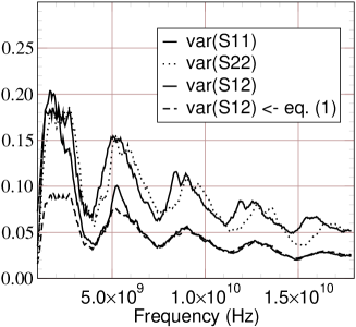
Figure 1: Experimental evidence for a hard relation between the variances of multi-port $S$-parameters in MSC. The dashed curve is computed from the two reflection parameters using eq. (1).

Outline of the paper

In section II, we summarise the essentials of frequency domain electromagnetic theory as far as we need it in our analysis. In particular, we formulate a succinct theory of scattering and introduce an “inside out” scattering operator of a reverberating environment.

In section III, we show how a change in the environment of a linear multi-port system (typically, the interconnect part of some electronic system) influences the multi-port model parameters of the system. The same analysis can be carried through for a multi-port model of Scattering, Thévenin, Norton or Hybrid type. Therefore, we shall study a generic inhomogeneous linear model. The essential result of this section is that the induced model parameter perturbations are expressed in terms of the electromagnetic field scattering operator of that environment. It is convenient, but not necessary, to choose free space as a reference environment. In that case, we obtain expressions for the deviation of the multi-port model parameters due to any object in the system’s environment showing contrast with respect to free space. The environment scattering operator is then defined in the usual way as related to scattering with respect to vacuum.

If the environment is considered as a stochastic scatterer, the derived relation implies that there are stochastic fluctuations in the multi-port system’s $S$-parameter model. In order to characterise these fluctuations, we need a hypothesis about the nature of the stochastic environment. In section IV, we give the definition of what we call a Statistically Isotropic Environment (SIE). This postulate implies some interesting properties of the scattering operator of the environment. In particular, we find that the variances of the coefficients of a matrix representation of the scattering operator satisfy $\operatorname{var}(S_{pq})=(1+\delta_{pq})/N$, where $N$ is the finite dimension of the wave space in which the fluctuating part of the environment scattering operator works. Observe that this means that the scattering operator of the environment satisfies equation (1). At the time of developing our theoretical analysis, we were not aware of the fact that such statistically isotropic scattering problems had already received much attention in the literature on neutron scattering. In fact, the formula describing the structure of the variance of scattering coefficients is known as the Hauser-Feshbach formula . The theory of this formula has been formulated in various ways in the past (in particular the analysis of Mello and Friedman has many apparent similarities to our approach FriedmanMello ), however, our approach seems to lead to the same result in a more direct way. In the context of optical scattering in random media, the phenomena of enhanced backscattering leads to similar relations (KugaIshimaru Y. Kuga and A. Ishimaru, J. Opt. Soc. Am. vol. 1, 1984 p. 831). In addition, we use this elementary property of statistically isotropic scattering to find variance properties of parameters of models which are quite different in nature.

In section V, we show that, under certain circumstances, the properties of the environment scattering operator are inherited by the fluctuations in the parameters of a generic model for a multi-port system in that environment. This section, therefore, provides the theoretical foundation of the relation given in equation (1) but includes the results, obtained in an entirely different way, by the researchers from the University of Maryland. The conclusion of the Maryland analysis that there is an essential difference between scattering parameter variance ratios and impedance variance ratios is not confirmed by our analysis. This maybe due to the fact that our hypothesis of isotropic scattering environments is incompatible with their hypothesis of wave chaotic cavity environment.

In the appendices, we present some details of the demonstrations. In particular, we study the properties of statistically isotropic unit vectors in multi-dimensional complex vector spaces, which are essential for the theory of scattering by isotropic environments.

II Basic relations

We shall develop our theoretical analysis using time harmonic electromagnetic scattering theory. We want to study the modifications in the behaviour of an electronic system due to electromagnetic interactions with it’s environment. One type of such an interaction is related to the electromagnetic fields in the environment generated by external sources. Such fields induce signals in the system even when the system itself is passive. A second type of interaction is related to the electrical currents, carried by the active system itself, which generate electromagnetic fields in the system’s environment. These fields are scattered by the environment and, when partially reflected back to the system, induce signals which again modify the behaviour of the system. The latter situation is, in fact, the general one, because we can incorporate the source of some ambient field by extending our system to include an additional port on which a source is applied.

We consider configurations, of the general type illustrated in Fig. 2, where some electronic system, occupying a domain represented by $\Omega^{-}\subset\mathbb{R}^{3}$, resides in an environment, occupying the complementary domain represented by $\Omega^{-}=\mathbb{R}\setminus\overline{\Omega^{-}}$.

The “environment domain,” $\Omega^{+}$, is the unbounded complement $\mathbb{R}^{3}\setminus\Omega^{-}$ and contains either a reference distribution of reciprocal material or the actual one. In order to simplify the presentation of the ideas, we shall take the reference environment to be vacuum and suppose that $\partial\Omega^{-}$ has an open neighbourhood on which the vacuum Maxwell equations hold.

The “system domain,” $\Omega^{-}$, is further decomposed in an interconnect subdomain, in $D\subset\Omega^{-}$, and various port-regions, $\Omega_{P}=\Omega^{-}\setminus D$. The complete system consists of, possibly non-linear, electronic components, located in $\Omega_{P}$, connected to the interconnect subsystem. On each connected component of $\Omega_{P}$, the low frequency approximation of the electromagnetic field is assumed to hold. In the interconnect domain, we suppose that all dielectrics and conductors are linear and reciprocal.

Figure 2: Electronic system decomposed as a linear multi-port interconnect system in $D$ terminated with electronic components in $\Omega_{P}$.

The electromagnetic fields in the configuration satsify the frequency domain Maxwell equations,

$$\nabla\times H-j\omega\varepsilon E =J$$

$$\nabla\times E+j\omega\mu H =0$$

the constitutive coefficients, $\varepsilon$ and $\mu$ are supposed to be real symmetric tensor functions, representing lossless reciprocal media. In the following sections, we concentrate on the model of the interconnect system and shall only consider fields corresponding to port excitations. That means that the distributions of electric current source, $J$, vanish outside $\Omega_{P}$.

In particular, in the interconnect system domain, $D$, we use these properties to establish the Lorentz field reciprocity relation. If $\{E^{a},H^{a}\}$ and $\{E^{b},H^{b}\}$ are two electromagnetic states, satisfying the same source-free Maxwell equations in $D$, we have,

$$\int_{\partial\Omega_{P}}\nu\cdot(E^{a}\times H^{b}-E^{b}\times H^{a})\\ =\int_{\partial\Omega^{-}}\nu\cdot(E^{a}\times H^{b}-E^{b}\times H^{a})$$ (2)

without any constraints on the nature of the states in the exterior of $D$, i.e., the relation holds irrespective of the coefficients of the Maxwell equations in $\Omega_{P}$ and $\Omega^{+}$. In order to simplify the notations, we shall write electromagnetics fields as

$$\Psi =(E,H)$$

and denote forms of the Lorentz type by,

$$\operatorname{\mathcal{L}}_{\partial\Omega^{-}}(\Psi^{a},\Psi^{b}) =\int_{\partial\Omega^{-}}\nu\cdot(E^{a}\times H^{b}-E^{b}\times H^{a})$$

We shall use standard scattering theory for the scattering description of the environment. This is based on a decomposition of the traces on $\partial\Omega^{-}$ of any electromagnetic field, which can exist in the configuration, into two components,

$$\Psi =\Psi^{+}+\Psi^{-}$$

where $\Psi^{+}$ is the boundary limit of a solution of the source-free vacuum Maxwell equations (and outgoing radiation condition) in $\Omega^{+}$ and $\Psi^{-}$ is the boundary limit of a solution of the source-free vacuum Maxwell equations in $\Omega^{-}$. The fact that the sum of the two constituents corresponds to a field which satisfies a given system of Maxwell equations in $\Omega^{+}$, makes that they are related by,

$$\Psi^{-}=S\Psi^{+}$$

where $S$ is the scattering operator of the environment.

Note that, as a consequence of their definitions, we have for any pair of states of the same type,

$$\operatorname{\mathcal{L}}_{\partial\Omega^{-}}(\Psi^{a;+},\Psi^{b;+}) =0=\operatorname{\mathcal{L}}_{\partial\Omega^{-}}(\Psi^{a;-},\Psi^{b;-})$$

In the theoretical development of the following sections, we shall encounter Lorentz type integrals, $\operatorname{\mathcal{L}}_{\partial\Omega^{-}}(\Psi^{a},\Psi^{b;-})$, where $\Psi^{b;-}$ corresponds to a field satisfying the vacuum Maxwell equations in $\Omega^{-}$ and $\Psi^{a}$ to a general system of Maxwell equations. This is a frequently occurring case and the Lorentz type integral is equivalent to a convenient domain integral representation,

$$\operatorname{\mathcal{L}}_{\partial\Omega^{-}}(\Psi^{a},\Psi^{b}) =\int_{\Omega^{-}}(E^{b}\cdot J^{a})$$

where, assuming a configuration with dielectrics only, $J^{a}=J+[j\omega(\varepsilon-\varepsilon_{0})]E^{a}$ is called the electric contrast source distribution of the state $\Psi^{a}$.

III Deterministic interaction

In this section, we present the theory of the influence of a change in the environment on the model parameters of a linear multi-port system. We shall follow the general strategy as outlined in Michielsen15 . We represent the linear multi-port system by a mathematical model and study the relation between the model parameters and the properties of the environment (as represented by the model discussed in section II).

The frequency domain model of a linear $N$-port system has the following general form

$$y =\eta+Ax$$

where $x,y,\eta\in\mathbb{C}^{N}$ and $A:\mathbb{C}^{N}\to\mathbb{C}^{N}$ a linear mapping. The vector $x$, represents the the excitations of the multi-port system and the vector $y$ represents the responses of the multi-port system. The inhomogeneity, or “source” term, $\eta$ represents the response of the system when there are no excitations on the system’s ports, i.e., $\eta$ represents sources internal to the multi-port system. Note, again, that viewed from the ports of the multi-port system the complete environment of the interconnect system is considered as being part of the multi-port system. This implies that the “internal” source $\eta$ represents electromagnetic fields generated by sources in the environment coupling to the interconnect system. The Thévenin, Norton, Hybrid and Scattering parameter models are all of this form and we can develop our theory independently of the specific type chosen. If needed, we shall label certain objects with $A$ which could then be replaced by $Z$ for a Thévenin model, $Y$ for a Norton model $H$ for a Hybrid model or $S$ for a scattering parameter model to specialise to a given case.

The model parameters are $\eta$ and $A$. These are the basic quantities we are interested in. For the purpose of this paper, though, we shall only consider the matrix $A$, because, in the context of reverberating environments, all the information we need follows from $A$-parameters. Indeed, if we include the input port of some emitting antenna in the environment as an additional port of our multi-port system, we can suppose that there are no sources in the environment of the resulting extended multi-port system, therefore we take

$$\eta=0$$

in the rest of this paper.

We consider a given $A$-parameter model of a multi-port system applying to its intended operational environment, say, for simplicity, free-space. It is now necessary, to know how a deviation from this intended environment translates into deviations of the model parameters. We will first carry out this analysis in a deterministic context where the perturbation is supposed to be completely known.

From now on, we shall denote the ideal (reference) model by

$$y =A^{0}x$$ (3)

and the true model by

$$y =Ax$$ (4)

A change in an environment can be modeled naturally as an electromagnetic scattering problem. So the aim of this section is to establish the relation between the scattering model of some electromagnetic environment and the matrix $A$ of the system’s multi-port model.

We shall now study electromagnetic field states in the configuration depicted in Fig. 2. Recall that $\partial\Omega^{-}$ is a closed, possibly multi-component, surface, separating the system from its environment and $\partial\Omega_{P}$ the union of the surfaces enclosing the various port regions of the system. The domain $D$ between these two surfaces contains the conductors and dielectrics of the interconnect system, whereas the domain exterior to the surface $\partial\Omega^{-}$ contains all deviations from the intended free space environment of the system.

Upon substitution of the quasi-static approximations on the topological components of $\Omega_{P}$ into the field reciprocity relation (2), we obtain (see appendix A) :

$${x^{b}}^{t}y^{a}-{x^{\mathstrut a}}^{t}y^{b} =\operatorname{\mathcal{L}}_{\partial\Omega^{-}}(\Psi^{a},\Psi^{b})$$ (5)

The Lorentz reciprocity relation (5) allows us to find integral representations for the difference $\Delta A=A-A^{0}$, if we choose the two states appropriately. In our case,

• $\Psi^{a}=\Psi^{0}_{p}$ corresponds to $x^{a}_{k}=\delta_{k-p}$ a unit excitation applied to one of the ports of the system in a free-space reference environment,

• $\Psi^{b}=\Psi_{q}$, a true state, where $\Psi_{q}$ corresponds to $x^{b}_{k}=\delta_{k-q}$, a unit excitation applied to one of the ports of the system in its true environment.

Substituting the model equations, (3) and (4), into the equation (5), we obtain for the above choices,

$$\sum_{kl}\delta_{(k-p)}A_{kl}\delta_{(l-q)}-\delta_{(k-q)}A^{0}_{kl}\delta_{(l-p)}=\operatorname{\mathcal{L}}_{\partial\Omega^{-}}(\Psi^{0}_{p},\Psi_{q})$$

and using the symmetry of the matrices $A$ (reciprocla media outside the port-regions $\Omega_{P}$) in the two states

$$\Delta A_{pq} =\operatorname{\mathcal{L}}_{\partial\Omega^{-}}(\Psi^{0}_{p},\Psi_{q})$$ (6)

Following the scattering theory developed in section II, the field $\Psi_{q}$ can be decomposed on $\partial\Omega^{-}$ into a part $\Psi_{q}^{+}=\Psi_{q}^{0}$, satisfying the same equations as $\Psi^{0}_{p}$ in the exterior of $\partial\Omega^{-}$, and a part $\Psi_{q}^{-}$, satisfying the free-space equations in $\Omega^{-}$. In addition, there exists a scattering operator between these fields

$$\Psi_{q}=\Psi_{q}^{0}+S\Psi_{q}^{0}$$

Substituting this into (6) and using $\operatorname{\mathcal{L}}_{\partial\Omega^{-}}(\Psi^{0}_{p},\Psi^{0}_{q})=0$, we get

$$\Delta A_{pq} =\operatorname{\mathcal{L}}_{\partial\Omega^{-}}(\Psi_{p}^{0},S\Psi_{q}^{0})$$

This relation can be discretised using a basis $\{\psi_{k}^{-}\}$,

$$\Delta A_{pq} =\sum_{kl}\operatorname{\mathcal{L}}_{\partial\Omega^{-}}(\Psi_{p}^{0},\psi_{k}^{-})S_{kl}\operatorname{\mathcal{L}}_{\partial\Omega^{-}}(\Psi_{q}^{0},\psi_{l}^{-})$$

$$=\sum_{kl}L_{pk}S_{kl}L_{ql}$$ (7)

where we introduced the port-related linear forms $L_{p}$ defined by $L_{p}(\psi)=\operatorname{\mathcal{L}}_{\partial\Omega^{-}}(\Psi^{0}_{p},\psi)$, which have coefficients $L_{pk}=\int_{\Omega^{-}}(e^{-}_{k}\cdot J^{0}_{p})$ in the chosen basis $\{\psi_{k}\}$ and $J^{0}_{p}$ is the contrast current distribution corresponding to an excitation $x_{k}=\delta_{k-p}$ in the free-space environment (Note that in these expressions $\langle j,e\rangle=\int(j\cdot e)$ has no complex conjugation and should not be confused with the $L^{2}$ inner product $(a,b)=\langle a,\overline{b}\rangle$). This last equation constitutes the searched for relation between the perturbation of the $A$-parameters and the scattering model of the environment.

IV Scattering operator of a statistically isotropic reverberating environment

In the previous section, we established the relation between the perturbations of a linear system’s multi-port $A$-parameter model and the scattering model of that system’s environment. In practice, the true environment of a system is not completely known. It is possible to account for this by replacing the scattering operator of the environment by a stochastic operator. In principle, one would like to derive the characteristics of this stochastic operator through mathematical analysis of scattering problems. However, with the present state of mathematics it seems impossible to obtain such properties from first principles. Therefore, we shall postulate a minimal set of properties of this scattering operator, such as to reflect in the most natural way what we understand by a statistically isotropic reverberating environment.

In the first place, we identify a decomposition of the environment’s scattering operator into a fixed average part, $S^{\mathit{av}}$, and a fluctuating part with mean zero, $S^{\mathit{flct}}$,

$$S=S^{\mathit{av}}+S^{\mathit{flct}}$$

The fixed part induces, according to the preceding sections, a fixed average deviation from the multi-port model as compared to the wanted ideal environment. The fluctuating part is the one we are interested in here. In analogy with what can be found in canonical geometries (see MichielsenFiachetti2005 ), the fluctuating part of the environment scattering operator is taken to be finite dimensional. This finite dimension grows with frequency in a way which depends on the actual geometry of the environment. This can be understood physically as being due to the fact that in reverberating environments there is a finite number of propagating modes reaching the fluctuating parts of the environment and coming back into the domain $\Omega^{-}$. The remaining part of the (countably infinite) number of basis functions on $\partial\Omega^{-}$, does not radiate into the fluctuating environment and hence does not play a rôle in the fluctuating part of the scattering operator. An example of this can be found in conventional mode stirred chambers, where the mode stirrer is in one part of the chamber and only linear combinations of a very specific and finite set of plane wave fields, i.e., those corresponding to propagating wave guidemodes reflected by a short-circuit wall, give non-negligeable fields incident on the mode stirrer.

In the following development, we shall only talk of this zero-mean, fluctuating, part of the total scattering operator of the stochastic environment which, for simplicity, we continue to write as $S$. The dimension of the complex propagating wave subspace, spanned by the “propagating modes,” will be denoted by $N$.

Definition IV.1.

A Statistically Isotropic Environment (SIE) is such that the fluctuating part of the scattering matrix, representing the contrast of the environment with respect to a free space environment, constitutes a spectrally isotropic stochastic unitary matrix.

This definition uses a specific stochastic matrix, tailored to our needs.

Definition IV.2 (Spectrally isotropic stochastic matrix).

Let $S:\mathbb{C}^{N}\to\mathbb{C}^{N}$ be a stochastic linear transformation. We call this transformation spectrally isotropic if it has a spectral representation

$$S=\sum_{\lambda}s_{\lambda}\Pi_{\lambda}$$

with stochastic multipliers $s_{\lambda}$ and stochastic rank 1 operators of the form $\Pi_{\lambda}=v_{\lambda}v_{\lambda}^{t}$ (transpose with respect to the hermitean inner product), where each $v_{\lambda}$ is an isotropic unit vector (see appendix B).

Moreover, all the spectral multipliers, $s_{\lambda}$, and the vectors, $v_{\lambda}$, are mutually statistically independent. In addition, we assume that all eigenvalues are identically distirbuted stochastic variables, i.e., $\forall\lambda\;\operatorname{\mathbb{E}}(a_{\lambda})=0$ and $\operatorname{\mathbb{E}}(|a_{\lambda}|^{2})=\rho^{2}$.

In the context of environment scattering, $\rho$ will be called the environment’s effective reflection coefficient.

The inspiration for the above definitions comes from the interpretation we can give to a spectral decomposition. A linear combination of waves outgoing from the domain $\Omega^{-}$, which lies in a single eigenspace of the scattering operator, will be reflected by the environment as exactly the same linear combination modulo only a scalar multiplier $s_{\lambda}(\theta)$. If we choose the environment to be perfectly isotropic, we would require that there exist no preference whatsoever of the various eigenspaces for any subspace of $\mathbb{C}^{N}$ and, moreover, that the eigenvalues are statistically the same for any eigenspace.

An important consequence of this postulate is derived from the properties of the cartesian components of isotropic unit vectors.

Proposition IV.3.

Let $z$ be a stochastic unit vector, in $N$ dimensional complex vector space, such that the real and imaginary parts constitute a uniformly distributed vector on the unit sphere in $2N$ real dimensions. Then the modules of the complex cartesian components, $z_{k}$, satisfy:

$$\operatorname{\mathbb{E}}(|z_{k}|^{2}) =\frac{1}{N}$$

$$\operatorname{\mathbb{E}}(|z_{k}|^{4}) =2\frac{1}{N^{2}}+\mathcal{O}(N^{-3})\quad\text{if $N\to\infty$}$$

$$\operatorname{\mathbb{E}}(|z_{k}|^{2}|z_{l}|^{2}) =\operatorname{\mathbb{E}}(|z_{k}|^{2})\operatorname{\mathbb{E}}(|z_{l}|^{2})+\mathcal{O}(N^{-3})\quad\text{if $k\not=l$ and $N\to\infty$}$$

Proof.

Let $z_{k}=x+iy$, with $x$ and $y$ cartesian components of an isotropic unit vector in $\mathbb{R}^{2N}$. We compute,

$$\operatorname{\mathbb{E}}(|z_{k}|^{2}) =\operatorname{\mathbb{E}}(x^{2}+y^{2})=\operatorname{\mathbb{E}}(x^{2})+\operatorname{\mathbb{E}}(y^{2})$$

using the results of appendix ??

$$=\frac{2}{2N}=\frac{1}{N}$$

$$\operatorname{\mathbb{E}}(|z_{k}|^{4}) =\operatorname{\mathbb{E}}(x^{4}+y^{4}+2x^{2}y^{2})$$

$$=\frac{6}{2N(2N+2)}+2\operatorname{\mathbb{E}}(x^{2}y^{2})$$

for the second term on the right hand side, we use the asymptotic estimate from appendix B proposition B.8

$$=\frac{6}{2N(2N+2)}+2\frac{1}{2N}\frac{1}{2N}+\mathcal{O}(N^{-3})$$

and, we also have $$\frac{6}{2N(2N+2)}=\frac{6}{4N^{2}}+\mathcal{O}(N^{-3})$$, so

$$=2/N^{2}+\mathcal{O}(N^{-3})$$

The third relation can also be shown by straightforward computation. Let $$z_{k}=x+iy z_{l}=u+iv$$ and , then, using proposition B.8 again, we obtain

$$\operatorname{\mathbb{E}}(|z_{k}|^{2}|z_{l}|^{2}) =\operatorname{\mathbb{E}}((x^{2}+y^{2})(u^{2}+v^{2}))$$

$$=\operatorname{\mathbb{E}}(x^{2}u^{2}+x^{2}v^{2}+y^{2}u^{2}+y^{2}v^{2})$$

$$=\operatorname{\mathbb{E}}(x^{2})\operatorname{\mathbb{E}}(u^{2})+\ldots+\mathcal{O}(\frac{1}{N^{3}})$$

$$=\operatorname{\mathbb{E}}(|z_{k}|^{2})\operatorname{\mathbb{E}}(|z_{l}|^{2})+\mathcal{O}(\frac{1}{N^{3}})$$

∎

Corollary IV.4.

The modules of the complex cartesian components of a complex isotropic vector $z\in\mathbb{C}^{N}$ satisfy asymptotically

$$\operatorname{\mathbb{E}}(|z_{k}|^{4}) =2\operatorname{\mathbb{E}}(|z_{k}|^{2})^{2}+\mathcal{O}(N^{-3})\quad\text{if $N\to\infty$}$$

The scattering matrix model of a SIE satisfies the following important relations.

Proposition IV.5.

Let $S$ be the (fluctuating part of the) scattering matrix of a SIE. Then,

• $\operatorname{\mathbb{E}}(S_{pq})=0$

• $\operatorname{\mathbb{E}}(S_{kl}\overline{S_{mn}})=(\delta_{k-m}\delta_{l-n}+\delta_{k-n}\delta_{l-m})\frac{\rho^{2}}{N}+\mathcal{O}(N^{-2})$

Proof.

As to the average:

$$\forall p,q\quad\operatorname{\mathbb{E}}(S_{pq}) =\sum_{\lambda}\operatorname{\mathbb{E}}(v^{\lambda}_{p}s^{\lambda}v^{\lambda}_{q})$$

because the average of a sum is the sum of the averages, using the statistical independence between $$s^{\lambda}$$ and the eigenvectors we obtain

$$\forall p,q\quad\operatorname{\mathbb{E}}(S_{pq}) =\sum_{\lambda}\operatorname{\mathbb{E}}(v^{\lambda}_{p}v^{\lambda}_{q})\operatorname{\mathbb{E}}(s^{\lambda})=0$$

The second property needs a bit more work,

$$\operatorname{\mathbb{E}}(S_{kl}\overline{S_{mn}}) =\sum_{\lambda\mu}\operatorname{\mathbb{E}}(v^{\lambda}_{k}s^{\lambda}v^{\lambda}_{l}\overline{v^{\mu}_{m}s^{\mu}v^{\mu}_{n}})$$

using again the statistical independence between eigenvalues and eigenvectors, we find

$$\operatorname{\mathbb{E}}(S_{kl}\overline{S_{mn}}) =\sum_{\lambda\mu}\operatorname{\mathbb{E}}(v^{\lambda}_{k}v^{\lambda}_{l}\overline{v^{\mu}_{m}}\overline{v^{\mu}_{n}})\delta^{(\lambda-\mu)}\operatorname{\mathbb{E}}(|s^{\lambda}|^{2})$$

As the joint probability of the cartesian components is a tensor product of even functions (see Appendix ??), there are only non vanishing contributions on the right hand side when the average is over even functions. Therefore, we get

$$\operatorname{\mathbb{E}}(S_{kl}\overline{S_{mn}}) =\sum_{\lambda}\begin{cases}\operatorname{\mathbb{E}}(|v^{\lambda}_{k}|^{2}|v^{\lambda}_{l}|^{2})\delta_{k-m}\delta_{l-n}\rho^{2}&k\not=n\\ \operatorname{\mathbb{E}}(|v^{\lambda}_{m}|^{2}|v^{\lambda}_{n}|^{2})\delta_{k-n}\delta_{l-m}\rho^{2}&k\not=m\end{cases}$$

using the asymptotics of proposition IV.3 and $$\lim_{N\to\infty}\sum_{\lambda}\mathcal{O}(N^{-3})=\mathcal{O}(N^{-2})$$, we obtain

$$\operatorname{\mathbb{E}}(S_{kl}\overline{S_{mn}}) =(\delta_{k-m}\delta_{l-n}+\delta_{k-n}\delta_{l-m})\frac{\rho^{2}}{N}+\mathcal{O}(N^{-2})$$

This yields the proposed relation. ∎

In fact, the proof given above shows that the structure of the matrix of variances of the scattering coefficients is particularly simple in the case of a SIE.

Corollary IV.6.

The variances of the scattering matrix of a SIE satisfy

• with $p\not=q$, $\operatorname{var}(S_{pq})=\frac{1}{2}\operatorname{var}(S_{pp})=\frac{1}{2}\operatorname{var}(S_{qq})$, when $N\to\infty$,

• $\operatorname{var}(S_{pq})=(\delta_{p-q}+1)\frac{\rho^{2}}{N}+\mathcal{O}(N^{-2})$

where $N$ is the dimension of the wave space in which the scattering matrix is expressed.

The essential result of this section is that the fluctuating part of the scattering operator of a Perfectly Isotropic Reverberating Environment (SIE) satisfies the relation (1). It is the purpose of the next section to show that, in a certain way, the induced fluctuations of multi-port $S$-parameters in such an environment inherit this basic relation.

V Induced perturbations of multi-port model parameters

With the definition of a SIE given in the preceding section and the results of section III, we are sufficiently equipped to characterise the nature of the stochastic perturbations of the $S$-parameter multi-port model of an equipment. In section III, the variations of the model parameters of a linear system, due to a variation of the electromagnetic environment, have been expressed in terms of bi-linear combinations of scalar products:

$$\Delta A_{pq} =\sum_{kl}L_{pk}S_{kl}L_{ql}=\sum_{k,l}\langle J^{0}_{p},e^{-}_{k}\rangle S_{kl}\langle J^{0}_{q},e^{-}_{l}\rangle$$ (8)

In this expression, $\{J^{0}_{p}\}$ is a set of current distributions, completely determined by the system in free space, and $\{e^{-}_{k}\}$ is a set of incident waves, chosen as a base for expansion of regular fields in the system domain $\Omega^{-}$.

The variances of the coefficients of the scattering operator in a SIE satisfy a simple relation (see IV). Because the fluctuations of the multi-port system’s $S$-parameters reflect properties of the SIE through the latter’s scattering operator, we might expect to find similar relations between the variances of these perturbations. That this follows indeed depends on the following result.

Proposition V.1.

Let $L$ be a matrix of which the rows are orthogonal, i.e., $\sum_{k}L_{pk}\overline{L}_{qk}=\delta_{(p-q)}\|L_{p}\|^{2}$, let $S$ be a spectrally isotropic matrix then the coefficients of the matrix $A=LSL^{t}$ have variances satisfying the relation

$$\lim_{N\to\infty}\operatorname{var}(A_{pq})=\lim_{N\to\infty}\sqrt{\operatorname{var}(A_{pp})\operatorname{var}(A_{qq})/4}$$

where $N$ is the dimension of the subspace in which the fluctuating part of the scattering operator works.

Proof.

We first show that the averages vanish. Substitution of the definitions gives

$$\operatorname{\mathbb{E}}(A_{pq}) =\operatorname{\mathbb{E}}(\sum_{k,l}L_{pk}S_{kl}L_{ql})$$

$$=\sum_{k,l}L_{pk}\operatorname{\mathbb{E}}(S_{kl})L_{ql}$$

$$=0$$

Therefore, the variances are computed as

$$\operatorname{var}(A_{pq}) =\operatorname{\mathbb{E}}(\sum_{k,l,m,n}L_{pk}S_{kl}L_{ql}\overline{L_{pm}S_{mn}L_{nl}})$$

$$=\sum_{k,l,m,n}L_{pk}S_{kl}L_{ql}\overline{L_{pm}L_{nl}}\operatorname{\mathbb{E}}(S_{kl}S_{mn})$$

using the results of proposition IV.5, we get

$$=\sum_{k,l,m,n}L_{pk}L_{ql}\overline{L_{pm}L_{qn}}(\delta_{k-m}\delta_{l-n}+\delta_{k-n}\delta_{l-m})\frac{\rho^{2}}{N}$$

$$=\sum_{k,l}[L_{pk}L_{ql}\overline{L_{pk}L_{ql}}+L_{pk}L_{ql}\overline{L_{pl}L_{qk}}]\frac{\rho^{2}}{N}$$

$$=[\|L_{p}\|^{2}\|L_{q}\|^{2}+\sum_{k,l}L_{pk}L_{ql}\overline{L_{pl}L_{qk}}]\frac{\rho^{2}}{N}$$

The second term on the right hand side vanishes due to the orthogonality of the rows except when $$p=q$$, then we get the same result as the first term on the right hand side. This shows,

$$\operatorname{var}(A_{pq}) =\begin{cases}\|L_{p}\|^{2}\|L_{q}\|^{2}\rho^{2}&p\not=q\\ 2\|L_{p}\|^{4}\rho^{2}&p=q\end{cases}$$

This implies, that with $p\not=q$,

$$\operatorname{var}(A_{pq})^{2} =\operatorname{var}(A_{pp})\operatorname{var}(A_{qq})/4$$

which is the result we had to prove. ∎

The orthogonality between the forms $L_{p}$, on which depends the theoretical proof of equation (1), can be obtained for different reasons. The relation of proposition V.1 between the variances can therefore appear in various different situations.

In fact, the orthogonality of the linear forms $L_{p}$ and $L_{q}$ is the orthogonality of the system’s radiation patterns corresponding to the excitations of the respective ports $p$ and $q$. This is equivalent to simple power-additivity of the resulting current distributions (see also MichielsenFiachetti2004a ). In other words, when the radiation power of the simultaneous excitation of ports $p$ and $q$ is the sum of the powers of the individual excitations, the proposed relation should hold (Here, we are neglecting the fact that for power additivity only the real part of the inner product of radiation patterns needs to vanish!).

We leave it as an open problem to find practical characterisations of situations where this happens. According to the variety of configurations where the result has been observed experimentally, the conditions are expected to be quite weak. This may be due to the fact that the relation is essentially an asymptotic relation and that in many configurations $N$ grows as $f^{3}$, i.e. the frequency need not be very high before the asymptotic estimates hold.

VI Estimating the coupling between ports in isotropic stochastic environments

In the variance ratios derived in the previous section, the coefficients which determine the actual fluctuations in the model coefficients did not appear. In practical situations, however, it is frequently necessary to be able estimate the variance of a coefficient describing the coupling between two ports. For that we need to be able to evaluate the quantities $\rho$ and $\|L_{p}\|$ appearing in the expressions.

The essential step is to observe that the norms of the port-bound linear forms $L_{p}$ give the free-space radiation power of the system under unit excitation at its $p$-th port. We elaborate this for the principal multi-port models to which our theory applies.

$$\|L_{p}\|^{2} =R_{\mathrm{rad;p}}$$ (Thévenin model)

$$\|L_{p}\|^{2} =G_{\mathrm{rad;p}}$$ (Norton model)

$$\|L_{p}\|^{2} =(1-|S_{pp}|^{2})C S$$ (-parameter model)

where $R_{\mathrm{rad;p}}$ is the port’s radiation resistance, $G_{\mathrm{rad;p}}$ the port’s radiation conductance and $(1-|S_{pp}|^{2})C$ the port’s mismatch times a radiation efficiency coefficient $C\leq 1$.

An isotropic stochastic environment is characterised by a single global coefficient $\rho$, which we called the environment’s effective reflection coefficient. We can determine this coefficient experimentally, using the $S$-parameter model for some ideal reference two-port system with perfectly adapted lossless antennas, i.e., $S_{pp}=0$ and $C=1$, we get

$$\rho^{2} =\operatorname{var}(S_{12})$$

because in that configuration we have $\|L_{1}\|^{2}=1=\|L_{2}\|^{2}$. It is of course possible to do a more realistic computation when the mismatch factors and radiation efficiencies of the antennas in the reference siutation are known. Of course, the Thévenin or Norton model could also be used if the radiation resistance or radiation conductance of the antennas were known. In practice, though, the scattering parameters are the most easily accessed by measurement.

To determine the coefficients $\|L_{p}\|^{2}$ for a port on an arbitrary system, port, we can put the system in a conventional mode stirred chamber and measure the variance statistic of $S_{pp}$ (or $R_{pp}$ or $G_{pp}$) over one turn of the mode stirrer. Together, with the $\rho$ obtained with the reference setup in the actual stochastic environment, we then have the variance of the coupling coefficients between any ports in the stochastic environment.

Conclusion

In this paper, we have developed a theoretical model for the fluctuations in the model parameters of linear multi-port systems induced by stochastic reverberating environments. This theory corroborates an experimentally observed correlation between the variances of the reflection coefficients and the variances of the transmission coefficients. In a certain way, the fluctuations in the reflection coefficients are shown to measure the strength of the coupling between a system port and the system’s environment. This gives a practical, quantitative, application of a familiar idea from antenna reciprocity, putting radiation and reception properties into correspondence. On the one hand these results can be used to judge on the quality of the statistical isotropy of the environment. On the other hand, the derived relations can also be applied, in such statistically isotropic environments, for estimating induced signal levels from only ambient field levels and reflection measurements.

The theory developed here should be compared to the development presented in ZhengHemmadyAntonsenAnlageOtt . The results presented there conflict with ours. Whereas in our analysis all multi-port models are handled in the same way, that reference singles out the impedance model as a special case. The apparent incompatibility of the results may be due to the fact that our hypothesis stating that the stochastic environment is characterised by a statistically isotropic scattering matrix appears to be incompatible with the hypothesis of a cavity with wave chaos as used in reference ZhengHemmadyAntonsenAnlageOtt .

Appendix A Low frequency field decompositions related to electronic ports

In this appendix, we present a field decomposition on $\partial\Omega_{P}$ and derive the consequences for surface integrals of Lorentz type.

As on each simply connected component of $\Omega_{P}$ we can use the low frequency approximation for the electromagnetic field, we have

$$\nabla\times E =0\Rightarrow E=-\nabla\varphi$$

$$\nabla\times H =J$$

where we used the Poincaré lemma. (If the component should not be simply connected, we can eliminate internal exclusions to arrive at a global potential.)

We want to relate Lorentz type integrals to multi-port $S$-parameters. Therefore, we have to proceed intwo steps: first relate fields to the usual multi-port quantities, voltage and current, and then field decompositions to the multi-port wave decompositions used in $S$-parameter models.

The first relation is found by subsituting the low frequency approximation into the surface integral

$$\int_{S}n\cdot(E^{a}\times H^{b})=-V^{a}\cdot I^{b}$$

where $V^{a}$ is the vector of port voltages and $I^{b}$ a vector of port currents. This derivation is classical (see deHoopI ; Michielsen15 ).

In the vector space, $\mathbb{C}^{2n}$ of all pairs $(V,I)$, we define the projection operators,

$$\Pi^{\pm}:X\to X^{\pm}$$

by

$$\Pi^{\pm} =\frac{1}{2}\begin{bmatrix}\mathbb{I}&\pm R\mathbb{I}\\ \pm R^{-1}\mathbb{I}&\mathbb{I}\end{bmatrix}$$ (9)

where $R$ is some positive real constant.

Let $\phi^{\pm}=V^{\pm}/\sqrt{2R}$ where $V^{\pm}$ is the voltage component in the image of $\Pi^{\pm}$. Then using

$$V =V^{-}+V^{+}$$

$$I =I^{-}+I^{+}$$

and $I^{\pm}=\pm R^{-1}V^{\pm}$ we easily compute

$$-V^{a}\cdot I^{b}+V^{b}\cdot I^{a} =\phi^{a;+}\cdot\phi^{b;-}-\phi^{b;+}\cdot\phi^{a;-}$$

The results of this appendix can then be summarised in the following equation

$$\int_{S}n\cdot(E^{a}\times H^{b}-E^{b}\times H^{a})=\\ \phi^{a;+}\cdot\phi^{b;-}-\phi^{b;+}\cdot\phi^{a;-}$$ (10)

Observe that this relation is the low-frequency analogue of the field decomposition used in electromagnetic scattering theory.

Appendix B Some results from probability theory

In this paper, we use classical probability theory as presented in textbooks. However, the specific results we need our theory are not easily found in the literature. Therefore, we feel obliged to present a succinct presentation dedicated to the analysis of stochastic unit vectors.

Mathematical probability theory is formulated in terms of Borel measures on topological spaces. In applications, though, a probability space is frequently given as a differentiable $n$-dimensional manifold, $X$, and the probability measure as a “volume element,” i.e., an exterior differential $n$-form, $\tau\in\Lambda^{n}$, on this manifold. If this is the case, we shall speak of a probability manifold, written as $(X,\tau)$. the measure of a set $U\subset X$ is then represented by $\langle\tau,U\rangle=\int_{U}\tau$.

Marginal probabilities for charts on probability manifolds

Charts on a manifold define coordinate functions on open subsets of the manifold. Therefore, the individual coordinates can be interpreted as stochastic variables (after “normalisation” relative to the measure of the open subset in question). The probability that a certain coordinate will be in a given interval of $\mathbb{R}$ is the probability measure of the subset of the manifold for which the points have the chosen coordinate in that interval.

Definition B.1.

Let $\varphi:X\supset U\to V\subset\mathbb{R}^{n}$ be a chart on a probability manifold $(X,\tau)$ of dimension $n$. The probability that $\varphi^{k}\in A\subset\mathbb{R}$ is defined by

$$\mathbb{P}_{\varphi^{k}}(A)=\langle\tau,\varphi^{-1}[V\cap(\pi^{k})^{-1}[A]]\rangle/\langle\tau,U\rangle$$

where $\pi_{k}:\mathbb{R}^{n}\ni x\mapsto x^{k}$ is the projection on the $k$-th component (note, $\varphi^{k}=\pi^{k}\circ\varphi$ and hence we might have written $(\varphi^{k})^{-1}$, but we prefer the explicit representation here to make appear the intermediate subset $V\cap(\pi^{k})^{-1}[A]$).

We can establish a marginal probability density in the following way

Proposition B.2.

The $k$-th marginal probability density, $\mu^{k}_{\varphi}\in\Lambda^{n}$, of a chart, $\varphi:X\supset U\to V\subset\mathbb{R}^{n}$, on an $n$-dimensional probability manifold, $(X,\tau)$, is defined by

$$\forall A\subset\mathbb{R}\;\langle\mu^{k}_{\varphi},A\rangle_{\mathbb{R}}=\langle\tau,\varphi^{-1}[V\cap\pi_{k}^{-1}[A]]\rangle_{X}/\langle\tau,U\rangle_{X}$$

Proof.

In fact, the only new thing with respect to the above definition is the fact that densities are uniquely defined by their evaluation on integration domains. ∎

Isotropic stochastic unit vectors

In this section, we investigate the properties of what we call isotropic stochastic unit vectors in $\mathbb{R}^{n}$. (This is not a real restriction as a unit vector $z$ in Hermitean $\mathbb{C}^{n}$, with $\|z\|_{\mathbb{C}^{n}}=\sqrt{\sum_{k}\Re(z_{k})^{2}+\Im(z_{k})^{2}}$, is also a unit vector in Euclidean $\mathbb{R}^{2n}$.)

Definition B.3.

A stochastic unit vector in $\mathbb{R}^{n}$ is defined by a probability manifold $(S^{n-1}_{1},\tau)$, where $\langle\tau,S^{n-1}_{1}\rangle=1$ and $\tau$ some density on the unit sphere $S^{n-1}_{1}$. An isotropic stochastic unit vector is defined by the normalised measure on the unit sphere induced by the, rotation invariant, Euclidean norm on $\mathbb{R}^{n}$, $\tau_{S^{n-1}_{1}}$, i.e., $\tau=\tau_{S^{n-1}_{1}}/|S^{n-1}_{1}|$.

Proposition B.4.

The cartesian components of an isotropic stochastic unit vector in $\mathbb{R}^{n}$ are stochastic variables $z\in[-1,+1]$ with a probability density $p(z)dz$, and

$$p(z)=(1-z^{2})^{(n-3)/2}\Gamma(n/2)/\sqrt{\pi}\Gamma((n-1)/2)$$

Proof.

We use the expression of proposition B.2 for the marginal probability measure of probability measures given as densities on manifolds. We obtain, $\forall A\subset(-1,1)$,

$$\langle\mu^{k}_{\varphi},A\rangle =\langle\sqrt{1-z^{2}}^{n-3}\tau_{S^{n-1}_{1}}\wedge dz,S^{n-1}_{1}\times A\rangle/|S^{n}_{1}|$$

$$=\langle\sqrt{1-z^{2}}^{n-3}\frac{|S^{n-2}|}{|S^{n-1}|}dz,A\rangle_{\mathbb{R}}$$

using $$\frac{|S^{n-2}|}{|S^{n-1}|}=\Gamma(n/2)/\sqrt{\pi}\Gamma((n-1)/2)$$, we get,

$$=\langle(1-z^{2})^{(n-3)/2}\Gamma(n/2)/\sqrt{\pi}\Gamma((n-1)/2)dz,A\rangle_{\mathbb{R}}$$

∎

We obtain the first few moments

Corollary B.5.

A cartesian component, $x_{k}$, of an isotropic unit vector in $x\in\mathbb{R}^{n}$ has the following moments,

$$m_{1}(x_{k}) =0$$

$$m_{2}(x_{k}) =\frac{1}{n}\quad\text{(equi-partition of variances)}$$

$$m_{3}(x_{k}) =0$$

$$m_{4}(x_{k}) =\frac{3}{n(n+2)}$$

Proof.

The moments have the following integral representation,

$$m_{p}(x_{k})=\int_{z=-1}^{1}z^{p}(1-z^{2})^{(n-3)/2}dz\frac{\Gamma(n/2)}{\sqrt{\pi}\Gamma((n-1)/2)}$$

As the integrand is an even function on $(-1,1)$, the odd moments all vanish. The even moments can be found as twice the integral over $(0,1)$, which leads to standard integrals.

$$m_{2}(x_{k}) =2\int_{z=0}^{1}z^{2}(1-z^{2})^{(n-3)/2}dz\frac{\Gamma(n/2)}{\sqrt{\pi}\Gamma((n-1)/2)}$$

$$=2\frac{\sqrt{\pi}\Gamma((n-1)/2)}{2\Gamma((n+2)/2)}\frac{\Gamma(n/2)}{\sqrt{\pi}\Gamma((n-1)/2)}$$

$$=\frac{\Gamma(n/2)}{2\Gamma(n/2+1)}=\frac{\Gamma(n/2)}{n\Gamma(n/2)}$$

$$=\frac{1}{n}$$

The fourth moment is computed in a similar way using

$$2\int_{z=0}^{1}z^{4}(1-z^{2})^{(n-3)/2}dz =\frac{3\sqrt{\pi}\Gamma((n-1)/2)}{4\Gamma((n+4)/2)}$$

using $$\Gamma((n+4)/2)=\frac{n}{2}(\frac{n}{2}+1)\Gamma(\frac{n}{2})$$

$$=\frac{3\sqrt{\pi}\Gamma((n-1)/2)}{n(n+2)\Gamma(n/2)}$$

∎

Proposition B.6.

The cartesian components of an isotropic unit vector in $\mathbb{R}^{n}$ tend to normal gaussian variables, $N(0,\frac{1}{n-3})$, when $n\to\infty$.

Proof.

With the following two standard results

$$\lim_{\tfrac{n-3}{2}\to\infty}(1-z^{2})^{(n-3)/2} =e^{-z^{2}(\tfrac{n-3}{2})}$$

$$\lim_{\tfrac{n-3}{2}\to\infty}\frac{\Gamma((n-3)/2+3/2)}{\Gamma((n-3)/2+1)} =\left(\frac{n-3}{2}\right)^{\frac{1}{2}}$$

we immediately get

$$\lim_{\tfrac{n-3}{2}\to\infty}(1-z^{2})^{(n-3)/2}\frac{\Gamma(n/2)}{\sqrt{\pi}\Gamma((n-1)/2)} =\frac{\sqrt{n-3}}{\sqrt{2\pi}}e^{-z^{2}(\tfrac{n-3}{2})}$$

$$=\frac{1}{\sigma\sqrt{2\pi}}e^{-\tfrac{z^{2}}{2\sigma^{2}}}$$

with $\sigma^{2}=1/(n-3)$. ∎

Proposition B.7.

The joint probability distribution of any $m$ cartesian components of an isotropic stochastic unit vector in $n$ real dimensions, is given by the probability density function

$$p(x^{1},\ldots,x^{m})=\frac{|S^{n-m-1}|}{|S^{n-1}|}\Pi_{k=0}^{m-1}(1-(x^{n-k})^{2})^{(n-k-3)/2}$$

Proof.

The proof follows the same reasoning as for the 1D marginal distribution. We start with the joint probability of two cartesian components. We know the density on the unit sphere $S^{n-1}_{1}$, in natural coordinates,

$$\tau_{S^{n-1}_{1}} =\tau_{S^{n-2}_{\sin(\theta^{n-1})}}\wedge d\theta^{n-1}$$

substitution of the corresponding expression for the first factor gives

$$=\sin(\theta^{n-1})^{n-2}\tau_{S^{n-3}_{\sin(\theta^{n-2})}}\wedge d\theta^{n-2}\wedge d\theta^{n-1}$$

$$=\sin(\theta^{n-1})^{n-2}\sin(\theta^{n-2})^{n-3}\tau_{S^{n-3}_{1}}\wedge d\theta^{n-2}\wedge d\theta^{n-1}$$

Substitution of $x^{n}=\cos(\theta^{n-1})$ then yields

$$\tau_{S^{n-1}_{1}}=(1-(x^{n})^{2})^{(n-3)/2}(1-(x^{n-1})^{2})^{(n-4)/2}\\ \tau_{S^{n-3}_{1}}\wedge dx^{n-1}\wedge dx^{n}$$ (11)

Using this result in the expression for marginal probability densities, we get, for any two cartesian components (The lack of symmetry in the joint probability density function is related to the fact that the components of an isotropic unit vector are not statistically independent and their squares have to sum up to unity.)

$$p(x^{n-1},x^{n})dx^{n-1}dx^{n}=(1-(x^{n})^{2})^{(n-3)/2}(1-(x^{n-1})^{2})^{(n-4)/2}\\ \frac{|S^{n-3}_{1}|}{|S^{n-1}_{1}|}dx^{n-1}dx^{n}$$ (12)

It should be clear from the above procedure, that we can do this for any number of dimensions and get the expression of the proposition. ∎

Proposition B.8.

Let $x$ and $y$ be two different cartesian components of an isotropic stochastic unit vector in $\mathbb{R}^{n}$,

$$\operatorname{\mathbb{E}}(xy) =0$$

$$\operatorname{\mathbb{E}}(x^{2}y^{2}) =\operatorname{\mathbb{E}}(x^{2})\operatorname{\mathbb{E}}(y^{2})+\mathcal{O}(n^{-3})$$

Proof.

The first relation is a simple consequence of the symmetry properties of the joint probability distribution. The complete proof of the asymptotic estimate in the second relation is very technical and too long for this paper. Here we content ourselves by observing that the limit distributions are Gaussian and, hence, the proposition gives the correct limits.

∎

References

- (1) A.T. de Hoop, The N-port receiving antenna and its equivalent network, Philips Research Reports (Special issue in honor of C. Bouwkamp) 30 (1974), 302∗.
- (2) C. Fiachetti, Modèles du champ électromagnétique aléatoire pour le calcul du couplage sur un équipement Électronique en chambre réverbérante à brassage de modes et validation expérimentale, Ph.D. thesis, Université de Limoges, Novembre 2002.
- (3) Cécile Fiachetti and Bas Michielsen, Electromagnetic random field models for the analysis of coupling inside mode tuned chambers, IEE Electronics Letters 39 (2003), no. 24, 1713–1714.
-
(4)
W.A. Friedman and P.A. Mello, "information theory and statistical nuclear
reactions.
I. many-channel case and Hauser-Feshbach formula", Annals of Physics (1984). - (5) I. Junqua, F. Issac, B. Michielsen, and C. Fiachetti, Relation between variances of scattering parameters at an equipment port in a reverberating chamber, Proc. Int. Zürich EMC Symposium, February 2003, pp. 233–238.
- (6) Y. Kuga and A. Ishimaru, J. Opt. Soc. Am. (1984).
- (7) T.H. Lehman, A statistical theory of electromagnetic fields in complex cavities, Interaction Notes, May 1993.
- (8) Bas Michielsen and Cécile Fiachetti, Covariance operators, green functions and canonical stochastic fields, Proc. URSI International Symposium on Electromagnetic Theory, June 2004, pp. 299–301.
- (9) , Covariance operators, Green functions and canonical stochastic fields, Radio Science 40 (2005), no. 5, 1–12.
- (10) B.L. Michielsen, A new approach to electromagnetic shielding, Proc. Int. Zürich EMC Symposium, March 1985, pp. 509–514.
- (11) X. Zheng, S. Hemmady, T. Antonsen, S. Anlage, and E. Ott, Characterization of fluctuations of impedance and scattering matrices in wave chaotic scattering, Physical Review E 73 (2006), no. 046208, 046208–1 – 6.