Numerical study of a multiscale expansion of KdV and Camassa-Holm equation

Abstract.

We study numerically solutions to the Korteweg-de Vries and Camassa-Holm equation close to the breakup of the corresponding solution to the dispersionless equation. The solutions are compared with the properly rescaled numerical solution to a fourth order ordinary differential equation, the second member of the Painlevé I hierarchy. It is shown that this solution gives a valid asymptotic description of the solutions close to breakup. We present a detailed analysis of the situation and compare the Korteweg-de Vries solution quantitatively with asymptotic solutions obtained via the solution of the Hopf and the Whitham equations. We give a qualitative analysis for the Camassa-Holm equation

1. Introduction

It is well known that the solution of the Cauchy problem for the Hopf equation

(1.1) $$u_{t}+6uu_{x}=0,\quad u(x,t=0)=u_{0}(x),\;\;x\in\mathbb{R},\;t\in\mathbb{R}^{+}$$

reaches a point of gradient catastrophe in a finite time. The solution of the viscosity or conservative regularization of the above hyperbolic equation display a considerably different behavior. Equation (1.1) admits an Hamiltonian structure

$$u_{t}+\{u(x),H_{0}\}\equiv u_{t}+\partial_{x}\frac{\delta H_{0}}{\delta u(x)}=0,\quad$$

with Hamiltonian and Poisson bracket

$$H_{0}=\int u^{3}\,dx,\quad\{u(x),u(y)\}=\delta^{\prime}(x-y),$$

respectively. All the Hamiltonian perturbations up to the order $\epsilon^{4}$ of the hyperbolic equation (1.1) have been classified in [10]. They are parametrized by two arbitrary functions $c(u)$, $p(u)$

(1.2) $$\begin{split}&u_{t}+6u\,u_{x}+\frac{\epsilon^{2}}{24}\left[2c\,u_{xxx}+4c^{\prime}u_{x}u_{xx}+c^{\prime\prime}u_{x}^{3}\right]+\epsilon^{4}\left[2p\,u_{xxxxx}\right.\\ &\\ &\left.+2p^{\prime}(5u_{xx}u_{xxx}+3u_{x}u_{xxxx})+p^{\prime\prime}(7u_{x}u_{xx}^{2}+6u_{x}^{2}u_{xxx})+2p^{\prime\prime\prime}u_{x}^{3}u_{xx}\right]=0,\end{split}$$

where the prime denotes the derivative with respect to $u$. The corresponding Hamiltonian takes the form

$$H=\int\left[u^{3}-\epsilon^{2}\frac{c(u)}{24}u_{x}^{2}+\epsilon^{4}p(u)u_{xx}^{2}\right]\,dx$$

For $c(u)=12$, $p(u)=0$ one obtains the Korteweg - de Vries (KdV) equation $u_{t}+6uu_{x}+\epsilon^{2}u_{xxx}=0$, and for $c(u)=48u$ and $p(u)=2u$ the Camassa-Holm equation up to order $\epsilon^{4}$; for generic choices of the functions $c(u)$, $p(u)$ equation (LABEL:riem2) is apparently not an integrable PDE. However it admits an infinite family of commuting Hamiltonians up to order $O(\epsilon^{6}).$

The case of small viscosity perturbations of one-component hyperbolic equations has been well studied and understood (see [1] and references therein), while the behavior of solutions to the conservative perturbation (LABEL:riem2) to the best of our knowledge has not been investigated after the point of gradient catastrophe of the unperturbed equation except for the KdV case, [18, 23, 7].

In a previous paper [13] (henceforth referred to as I) we have presented a quantitative numerical comparison of the solution of the Cauchy problem for KdV

(1.3) $$u_{t}+6uu_{x}+\epsilon^{2}u_{xxx}=0,\quad u(x,0)=u_{0}(x),$$

in the small dispersion limit $\epsilon\rightarrow 0$, and the asymptotic formula obtained in the works of Lax and Levermore [18], Venakides [23] and Deift, Venakides and Zhou [7] which describes the solution of the above Cauchy problem at the leading order as $\epsilon\rightarrow 0$. The asymptotic description of [18],[7] gives in general a good approximation of the KdV solution, but is less satisfactory near the point of gradient catastrophe of the hyperbolic equation. This problem has been addressed by Dubrovin in [10], where, following the universality results obtained in the context of matrix models by Deift et all [8], he formulated the universality conjecture about the behavior of a generic solution to the Hamiltonian perturbation (LABEL:riem2) of the hyperbolic equation (1.1) near the point $(x_{c},t_{c},u_{c})$ of gradient catastrophe for the solution of (1.1). He argued that, up to shifts, Galilean transformations and rescalings, this behavior essentially depends neither on the choice of solution nor on the choice of the equation. Moreover, the solution near the point $(x_{c},t_{c},u_{c})$ is given by

(1.4) $$u(x,t,\epsilon)\simeq u_{c}+a\,\epsilon^{2/7}U\left(b\,\epsilon^{-6/7}(x-x_{c}-6u_{c}(t-t_{c}));c\,\epsilon^{-4/7}(t-t_{c})\right)+O\left(\epsilon^{4/7}\right)$$

where $a$, $b$, $c$ are some constants that depend on the choice of the equation and the solution and $U=U(X;T)$ is the unique real smooth solution to the fourth order ODE

(1.5) $$X=6T\,U-\left[U^{3}+(\frac{1}{2}U_{X}^{2}+U\,U_{XX})+\frac{1}{10}U_{XXXX}\right],$$

which is the second member of the Painlevé I hierarchy. We will call this equation PI2. The relevant solution is characterized by the asymptotic behavior

(1.6) $$U(X,T)=\mp(X)^{\frac{1}{3}}\mp\dfrac{2T}{X^{\frac{1}{3}}}+O(X^{-1}),\quad X\rightarrow\pm\infty,$$

for each fixed $T\in\mathbb{R}$. The existence of a smooth solution of (1.5) for all $X,T\in\mathbb{R}$ satisfying (1.6) has been recently proved by Claeys and Vanlessen [4]. Furthermore they study in [5] the double scaling limit for the matrix model with the multicritical index and showed that the limiting eigenvalues correlation kernel is obtained from the particular solution of (1.5) satisfying (1.6). This result was conjectured in the work of Brézin, Marinari and Parisi [2].

In this paper we address numerically the validity of (1.4) for the KdV equation, and we identify the region where this solution provides a better description than the Lax-Levermore, and Deift-Venakides-Zhou theory. As an outlook for the validity of (1.4) for other equations in the family (LABEL:riem2), we present a numerical analysis of the Camassa-Holm equation near the breakup point. While the validity of (1.4) can be theoretically proved using a Riemann-Hilbert approach to the small dispersion limit of the KdV equation [7] and recent results in [8],[4],[5], for the Camassa-Holm equation and also for the general Hamiltonian perturbation to the hyperbolic equation (1.1), the problem is completely open. Furthermore for the general equation (LABEL:riem2), the existence of a smooth solution for a short time has not been established yet. An equivalent analysis should also be performed for Hamiltonian perturbation of elliptic systems, in particular for the semiclassical limit of the focusing nonlinear Schrödinger equation [16],[21].

The paper is organized as follows. In section 2 we give a brief summary of the Lax-Levermore, and Deift-Venakides-Zhou theory and the multiscale expansion (1.4). In section 3 we present the numerical comparison between the asymptotic description based on the Hopf and Whitham solutions and the multiscale solutions with the KdV solution. In section 4 we study the same situation for the Camassa-Holm equation. In the appendix we briefly outline the used numerical approaches.

2. Asymptotic and multiscale solutions

Following the work of [18], [23] and [7], the rigorous theoretical description of the small dispersion limit of the KdV equation is the following: Let $\bar{u}(x,t)$ be the zero dispersion limit of $u(x,t,\epsilon)$, namely

(2.1) $$\bar{u}(x,t)=\lim_{\epsilon\rightarrow 0}u(x,t,\epsilon).$$

1) for $0\leq t<t_{c}$, where $t_{c}$ is a critical time, the solution $u(x,t,\epsilon)$ of the KdV Cauchy problem is approximated, for small $\epsilon$, by the limit $\bar{u}(x,t)$ which solves the Hopf equation

(2.2) $$\bar{u}_{t}+6\bar{u}\bar{u}_{x}=0.$$

Here $t_{c}$ is the time when the first point of gradient catastrophe appears in the solution

(2.3) $$\bar{u}(x,t)=u_{0}(\xi),\quad x=6tu_{0}(\xi)+\xi,$$

of the Hopf equation. From the above, the time $t_{c}$ of gradient catastrophe can be evaluated from the relation

$$t_{c}=\dfrac{1}{\min_{\xi\in\mathbb{R}}[-6u_{0}^{\prime}(\xi)]}.$$

2) After the time of gradient catastrophe, the solution of the KdV equation is characterized by the appearance of an interval of rapid modulated oscillations. According to the Lax-Levermore theory, the interval $[x^{-}(t),x^{+}(t)]$ of the oscillatory zone is independent of $\epsilon$. Here $x^{-}(t)$ and $x^{+}(t)$ are determined from the initial data and satisfy the condition $x^{-}(t_{c})=x^{+}(t_{c})=x_{c}$ where $x_{c}$ is the $x$-coordinate of the point of gradient catastrophe of the Hopf solution. Outside the interval $[x^{-}(t),x^{+}(t)]$ the leading order asymptotics of $u(x,t,\epsilon)$ as $\epsilon\rightarrow 0$ is described by the solution of the Hopf equation (2.3). Inside the interval $[x^{-}(t),x^{+}(t)]$ the solution $u(x,t,\epsilon)$ is approximately described, for small $\epsilon$, by the elliptic solution of KdV [14], [18], [23], [7],

(2.4) $$u(x,t,\epsilon)\simeq\bar{u}+2\epsilon^{2}\frac{\partial^{2}}{\partial x^{2}}\log\theta\left(\dfrac{\sqrt{\beta_{1}-\beta_{3}}}{2\epsilon K(s)}[x-2t(\beta_{1}+\beta_{2}+\beta_{3})-q];\mathcal{T}\right)$$

where now $\bar{u}=\bar{u}(x,t)$ takes the form

(2.5) $$\bar{u}=\beta_{1}+\beta_{2}+\beta_{3}+2\alpha,$$

(2.6) $$\alpha=-\beta_{1}+(\beta_{1}-\beta_{3})\frac{E(s)}{K(s)},\;\;\mathcal{T}=i\dfrac{K^{\prime}(s)}{K(s)},\;\;s^{2}=\frac{\beta_{2}-\beta_{3}}{\beta_{1}-\beta_{3}}$$

with $K(s)$ and $E(s)$ the complete elliptic integrals of the first and second kind, $K^{\prime}(s)=K(\sqrt{1-s^{2}})$; $\theta$ is the Jacobi elliptic theta function defined by the Fourier series

$$\theta(z;\mathcal{T})=\sum_{n\in\mathbb{Z}}e^{\pi in^{2}\mathcal{T}+2\pi inz}.$$

For constant values of the $\beta_{i}$ the formula (2.4) is an exact solution of KdV well known in the theory of finite gap integration [15], [9]. However in the description of the leading order asymptotics of $u(x,t,\epsilon)$ as $\epsilon\rightarrow 0$, the quantities $\beta_{i}$ depend on $x$ and $t$ and evolve according to the Whitham equations [24]

$$\dfrac{\partial}{\partial t}\beta_{i}+v_{i}\dfrac{\partial}{\partial x}\beta_{i}=0,\quad i=1,2,3,$$

where the speeds $v_{i}$ are given by the formula

(2.7) $$v_{i}=4\frac{\prod_{k\neq i}(\beta_{i}-\beta_{k})}{\beta_{i}+\alpha}+2(\beta_{1}+\beta_{2}+\beta_{3}),$$

with $\alpha$ as in (2.6). Lax and Levermore first derived, in the oscillatory zone, the expression (2.5) for $\bar{u}=\bar{u}(x,t)$ which clearly does not satisfy the Hopf equation. The theta function formula (2.4) for the leading order asymptotics of $u(x,t,\epsilon)$ as $\epsilon\rightarrow 0$, was obtained in the work of Venakides and the phase $q=q(\beta_{1},\beta_{2},\beta_{3})$ was derived in the work of Deift, Venakides and Zhou [7], using the steepest descent method for oscillatory Riemann-Hilbert problems [6]

(2.8) $$q(\beta_{1},\beta_{2},\beta_{3})=\frac{1}{2\sqrt{2}\pi}\int_{-1}^{1}\int_{-1}^{1}d\mu d\nu\frac{f_{-}(\frac{1+\mu}{2}(\frac{1+\nu}{2}\beta_{1}+\frac{1-\nu}{2}\beta_{2})+\frac{1-\mu}{2}\beta_{3})}{\sqrt{1-\mu}\sqrt{1-\nu^{2}}},$$

where $f_{-}(y)$ is the inverse function of the decreasing part of the initial data. The above formula holds till some time $T>t_{c}$ (see [7] or I for times $t>T$).

3) Fei-Ran Tian proved that the description in 1) and 2) is generic for some time after the time $t_{c}$ of gradient catastrophe [20].

In I we discussed the case $u_{0}(x)=-\mbox{sech}^{2}x$ in detail as an example. The main results were that the asymptotic description is of the order $\mathcal{O}(\epsilon)$ close to the center of the Whitham zone, but that the approach gives considerably less satisfactory results near the edges of the Whitham zone and close to the breakup of the corresponding solution to the Hopf equation. In the present paper we address the behavior near the point of gradient catastrophe of the Hopf solution in more detail. In Fig. 1 we show the KdV solution and the corresponding asymptotic solution as given above for several values of the time near the critical time $t_{c}$. It can be seen that there are oscillations before $t_{c}$, and that the solution in the Whitham zone provides only a crude approximation of the KdV solution for small $t-t_{c}$.

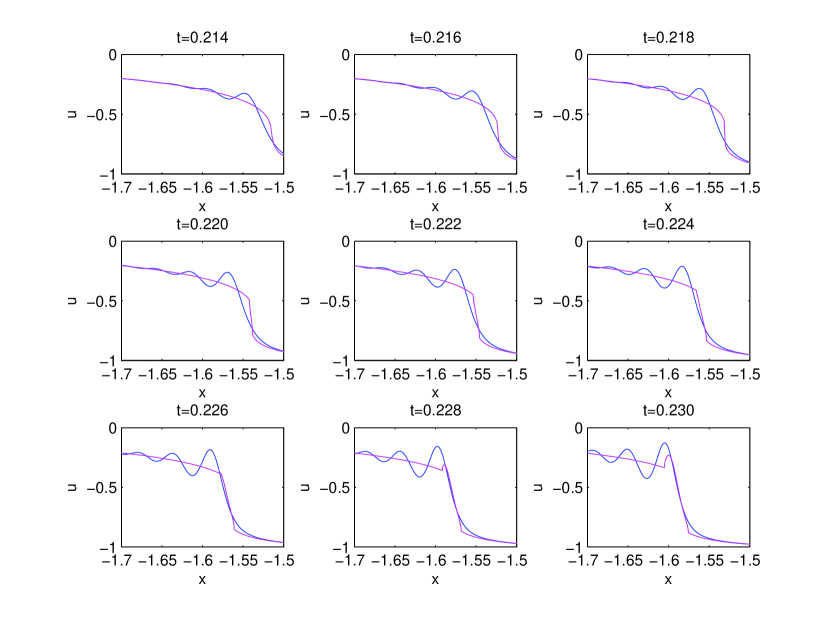
Figure 1. The blue line is the solution of the KdV equation for the initial data $u_{0}(x)=-1/\cosh^{2}x$ and $\epsilon=10^{-2}$, and the purple line is the corresponding leading order asymptotics given by formulas (2.3) and (2.4). The plots are given for different times near the point of gradient catastrophe $(x_{c},t_{c})$ of the Hopf solution. Here $x_{c}\simeq-1.524$, $t_{c}\simeq 0.216$.

The situation does not change in principle if we consider smaller values of $\epsilon$ as can be seen from Fig. 2. The solution shows the same qualitative behavior as in Fig. 1, just on smaller scales in $t$ and $x$.

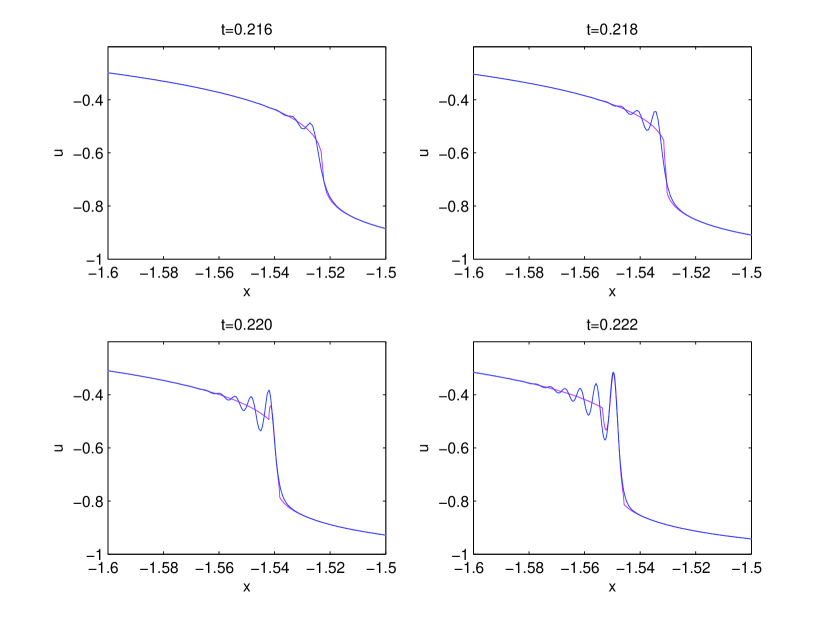
Figure 2. KdV solution and asymptotic solution for $\epsilon=10^{-3}$ close to the breakup time.

2.1. Multiscale expansion

We give a brief summary of the results in [10] relevant for the KdV case we are interested in here. Near the point of gradient catastrophe $(x_{c},t_{c},u_{c})$, the Hopf solution is generically given in lowest order by the cubic

(2.9) $$x-x_{c}\simeq 6(t-t_{c})u-k(u-u_{c})^{3},\quad k=-f_{-}^{\prime\prime\prime}(u_{c})/6,$$

because $6t_{c}+f_{-}^{\prime}(u_{c})=0$ and $f_{c}^{\prime\prime}(u_{c})=0$. Here $f_{-}(u)$ is the inverse of the decreasing part of the initial data $u_{0}(x)$. Now let us consider $h_{k}=\dfrac{\delta H_{k}}{\delta u}$ where $H_{k}$ are the KdV Hamiltonians such that $h_{k}=u^{k+2}/(k+2)!+O(\epsilon^{2})$. We have

$$h_{-1}=u,\;\;h_{0}=\dfrac{u^{2}}{2}+\dfrac{\epsilon^{2}}{6}u_{xx},\;\;h_{1}=\dfrac{1}{6}(u^{3}+\frac{\epsilon^{2}}{2}(u_{x}^{2}+2uu_{xx})+\dfrac{\epsilon^{4}}{10}u_{xxxx}),$$

and the KdV equation is obtained from $u_{t}+6\partial_{x}h_{0}=0$. Then

$$x=6tu+a_{0}h_{0}+a_{1}h_{1}+\dots a_{k}h_{k},$$

is a symmetry of the KdV equation [11]. Setting $a_{0}=0,$ $a_{1}=-f^{\prime\prime\prime}(u_{c})/6=k$ and $a_{k>2}=0$, and making the shift $t\rightarrow t-t_{c}$, $u\rightarrow u-u_{c}$ and the Galilean transformation $x\rightarrow x-x_{c}-6(t-t_{c})u_{c}$ we arrive at the fourth order equation of Painlevé type

(2.10) $$x-x_{c}-6(t-t_{c})u_{c}=6(t-t_{c})(u-u_{c})-k\left[(u-u_{c})^{3}+\epsilon^{2}(\dfrac{u_{x}^{2}}{2}+(u-u_{c})u_{xx})+\dfrac{\epsilon^{4}}{10}u_{xxxx}\right]$$

which is an exact solution of the KdV equation and can be considered as a perturbation of the Hopf solution (2.9) near the point of gradient catastrophe $(x_{c},t_{c},u_{c})$. The solution $u(x,t,\epsilon)$ of (2.10) is related to the solution $U(X,T)$ of (1.5) by the rescalings

(2.11) $$u(x,t,\epsilon)=u_{c}+\left(\dfrac{\epsilon}{k}\right)^{2/7}U(X,T)$$

where

(2.12) $$X=\dfrac{x-x_{c}-6u_{c}(t-t_{c})}{\epsilon^{\frac{6}{7}}k^{\frac{1}{7}}},\quad T=\dfrac{t-t_{c}}{\epsilon^{\frac{4}{7}}k^{\frac{3}{7}}}.$$

According to the conjecture in [10], the solution (2.11) is an approximation modulo terms $O(\epsilon^{\frac{4}{7}})$ to the solution of the Cauchy problem (1.3) for $(x,t,u)$ near the point of gradient catastrophe $(x_{c},t_{c},u_{c})$ of the hyperbolic equation (2.2).

3. Numerical comparison

In this section we will present a comparison of numerical solutions to the KdV equation and asymptotic solutions arising from solutions to the Hopf and the Whitham equations as well as the Painlevé I2 equation as given above. Since we control the accuracy of the used numerical solutions, see I, [17] and the appendix, we ensure that the presented differences are entirely due to the analytical description and not due to numerical artifacts. We study the $\epsilon$-dependence of these differences by linear regression analysis. This will be done for nine values of $\epsilon$ between $10^{-1}$ and $10^{-3}$. Obviously the numerical results are only valid for this range of parameters, but it is interesting to note the high statistical correlation of the scalings we observe. We consider the initial data

$$u_{0}(x)=-1/\cosh^{2}x.$$

For this initial data

(3.1) $$x_{c}=-\dfrac{\sqrt{3}}{2}+\log((\sqrt{3}-1)/\sqrt{2}),\;\;t_{c}=\dfrac{\sqrt{3}}{8},\;\;\;\;u_{c}=-2/3.$$

3.1. Hopf solution

We will first check whether the rescalings of the coordinates given in (2.11) are consistent with the numerical results. It is known that the Hopf solution provides for times $t\ll t_{c}$ an asymptotic description of the KdV solution up to an error of the order $\epsilon^{2}$. This means that the $L_{\infty}$-norm of the difference between the two solutions decreases as $\epsilon^{2}$ for $\epsilon\rightarrow 0$. For $t=0.1$ we actually observe this dependence. More precisely this difference $\Delta_{\infty}$ can be fitted with a straight line by a standard linear regression analysis, $-\log_{10}\Delta_{\infty}=-a\log_{10}\epsilon+b$ with $a=1.9979$, with a correlation coefficient of $r=0.99999$ and standard error $\sigma_{a}=4.1*10^{-3}$.

Near the critical time $t_{c}$ this picture is known to change considerably. Dubrovin’s conjecture [10] presented above suggests that the difference between Hopf and KdV solution near the critical point should scale roughly as $\epsilon^{2/7}$. In the following we will always compare solutions in the intervals

(3.2) $$[x_{c}+6u_{c}(t-t_{c})-\alpha\epsilon^{6/7},x_{c}+6u_{c}(t-t_{c})+\alpha\epsilon^{6/7}]$$

where $\alpha$ is an $\epsilon$-independent constant (typically we take $\alpha=3$).

Numerically we find at the critical time that the $L_{\infty}$-norm of the difference between Hopf and KdV solution scales like $\epsilon^{a}$ where $a=0.2869$ ($2/7=0.2857\ldots$) with correlation coefficient $r=0.9995$ and standard error $\sigma_{a}=6.9*10^{-3}$. Thus we confirm the expected scaling behavior within numerical accuracy. We also test this difference for times close to $t_{c}$. The relations (2.11) suggest, however, a rescaling of the time, i.e., to compare solutions for different values of $\epsilon$ at the same value of $T$. We compute the respective solutions for KdV times $t_{\pm}(\epsilon)=t_{c}\pm 0.1\epsilon^{4/7}$. Before breakup at $t_{-}$ we obtain $a=0.31$ with $r=0.999$ and $\sigma_{a}=9.8*10^{-3}$, i.e., as expected a slightly larger value than $2/7$. After breakup at $t_{+}$ we find $a=0.26$ with $0.9995$ and $\sigma_{a}=6.6*10^{-3}$. We remark that after the breakup time, the asymptotic solution is obtained by gluing the Hopf solution and the theta-functional solution (2.4).

These results indicate that the scalings in (2.11) are indeed observed by the KdV solution. We show the corresponding situation for $t_{-}$ for two values of $\epsilon$ in Fig. 3.

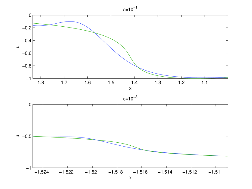
Figure 3. KdV solution (blue) and Hopf solution (green) at the times $t_{-}(\epsilon)$ in a rescaled interval for two values of $\epsilon$.

3.2. Multiscale solution

In Fig. 4 we show the numerical solution of the KdV equation for the initial data $u_{0}$ and the corresponding PI2 solution (2.11) for $\epsilon=10^{-2}$ close to breakup. It can be seen that the PI2 solution (2.11) gives a correct description of the KdV solution close to the breakup point. For larger values of $|x-x_{c}|$ the multiscale solution is not a good approximation of the KdV solution.

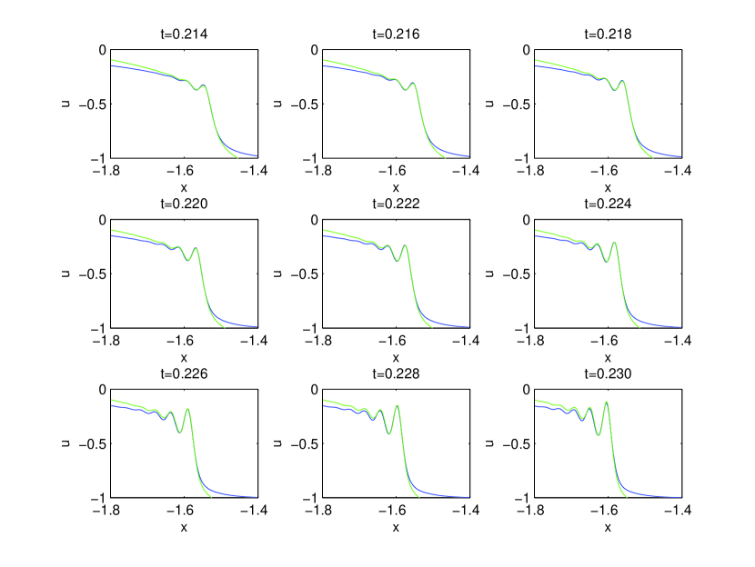
Figure 4. The blue line is the solution of the KdV equation for the initial data $u_{0}(x)=-1/\cosh^{2}x$ and $\epsilon=10^{-2}$, and the green line is the corresponding multiscale solution given by formula (2.11). The plots are given for different times near the point of gradient catastrophe $(x_{c},t_{c})$ of the Hopf solution. Here $x_{c}\simeq-1.524$, $t_{c}\simeq 0.216$.

A similar situation is shown in Fig. 5 for the case $\epsilon=10^{-3}$. Obviously the approximation is better for smaller $\epsilon$. Notice that the asymptotic description is always better near the leading edge than near the trailing edge.

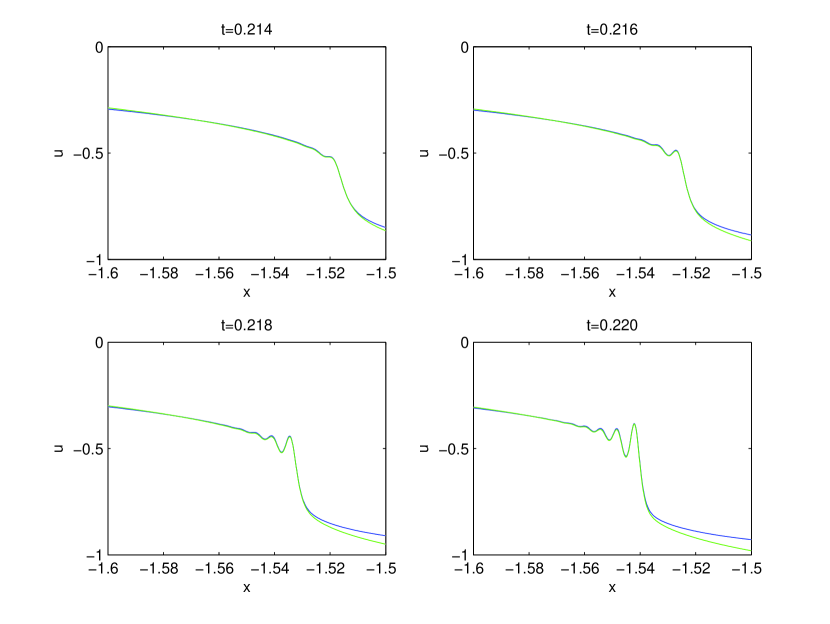
Figure 5. The blue line is the solution of the KdV equation for the initial data $u_{0}(x)=-1/\cosh^{2}x$ and $\epsilon=10^{-3}$, and the green line is the corresponding multiscale solution given by formula (2.11). The plots are given for different times near the point of gradient catastrophe $(x_{c},t_{c})$ of the Hopf solution.

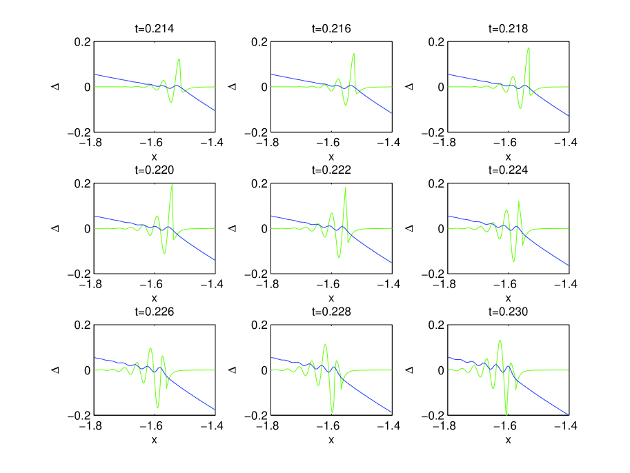
Figure 6. The blue line is the difference between the solution of the KdV equation for the initial data $u_{0}(x)=-1/\cosh^{2}x$ and $\epsilon=10^{-2}$ and the multiscale solution, and the green line is the difference between the asymptotic solution and the KdV solution. The plots are given for different times near the point of gradient catastrophe $(x_{c},t_{c})$ of the Hopf solution.

In Fig. 6 we plot in green the difference between the PI2 multiscale solution and the KdV solution and in blue the difference between the KdV solution and the asymptotic solutions (2.3) and (2.4). It is thus possible to identify a zone around $x_{c}$ in which the multiscale solution gives a better asymptotic description. The limiting values of this zone rescaled by $x_{c}$ are shown in Fig. 7 for the critical time. It can be seen that the zone always extends much further to the left (the direction of propagation) than to the right.

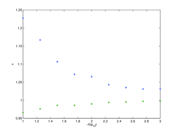
Figure 7. Limiting values of the zone where the multiscale solution provides a better asymptotic description of the KdV solution than the Hopf solution for $t=t_{c}$. The $x$ values are rescaled with $x_{c}$.

The width of this zone scales roughly as $\epsilon^{3/7}$, more precisely we find $\epsilon^{a}$ with $a=0.468$, $r=0.981$ and $\sigma_{a}=0.073$. We observe that the numerical scaling is smaller than the one predicted by the formula (2.12). The matching of the multiscale and the Hopf solution can be seen in Fig. 8.

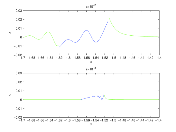
Figure 8. Difference of the KdV and the multiscale solution (blue) and the KdV and the Hopf solution (green) for the initial data $u_{0}(x)=-1/\cosh^{2}x$ at $t=t_{c}$ for two values of $\epsilon$.

For larger times, the asymptotic solution (2.3) and (2.4) gives as expected a better description of the KdV solution, see Fig. 9 for $\epsilon=10^{-3}$ and $t=0.226$. Close to the leading edge, the oscillations are, however, better approximated by the multiscale solution.

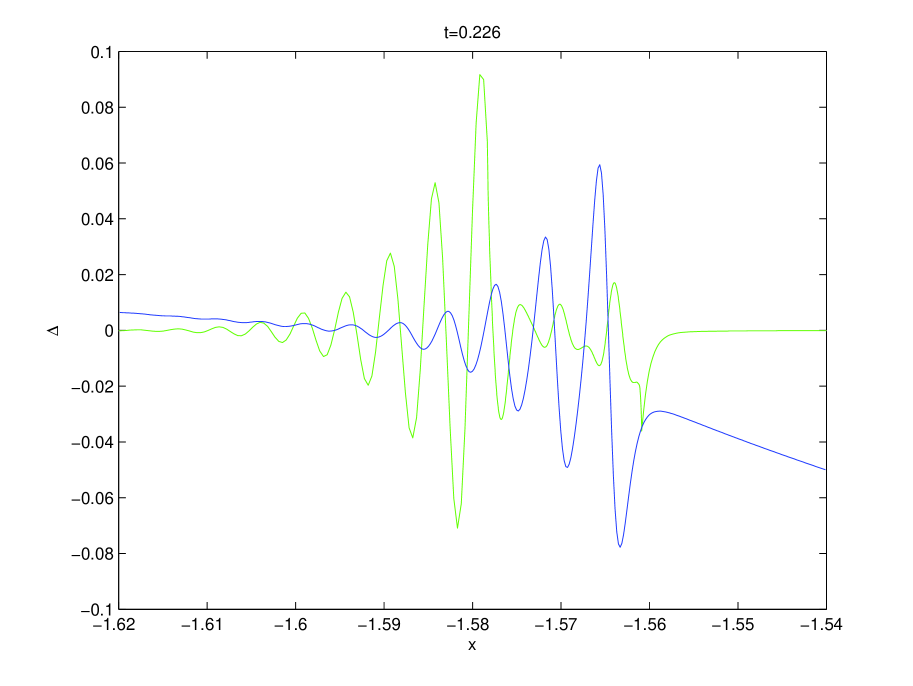
Figure 9. The blue line is the difference between solution of the KdV equation for the initial data $u_{0}(x)=-1/\cosh^{2}x$ and $\epsilon=10^{-3}$ and the multiscale solution, and the green line is the difference between the asymptotic solution and the KdV solution. The plots are given for $t=0.226$.

To study the scaling of the difference between the KdV and the multiscale solution, we compute the $L_{\infty}$ norm of the difference between the solutions in the rescaled $x$-interval (3.2) with $\alpha=3$. We find that this error scales at the critical time roughly like $\epsilon^{5/7}$. More precisely we find a scaling $\epsilon^{a}$ where $a=0.708$ ($5/7=0.7143\ldots$) with correlation coefficient $r=0.9998$ and standard error $\sigma_{a}=0.012$. Before breakup at the times $t_{-}(\epsilon)$ we obtain $a=0.748$ with $r=0.9996$ and $\sigma_{a}=0.016$, after breakup at the times $t_{+}(\epsilon)$ we get $a=0.712$ with $r=0.9999$ and $\sigma_{a}=6.2*10^{-3}$. Notice that the values for the scaling parameters are roughly independent of the precise value of the constant $\alpha$ which defines the length of the interval (3.2). For instance for $\alpha=2$, we find within the observed accuracy the same value. In [4] Claeys and Vanlessen showed that the corrections to the multiscale solution appear in order $\epsilon^{3/7}$. For the values of $\epsilon$ we could study for our KdV example, the corrections are apparently of order $\epsilon^{5/7}$.

4. Outlook

The Camassa-Holm equation [3] (see also [12])

(4.1) $$u_{t}+6uu_{x}-\epsilon^{2}(u_{xxt}+4u_{x}u_{xx}+2uu_{xxx})=0$$

admits a bi-Hamiltonian description after the following Miura-type transformation

(4.2) $$m=u-\epsilon^{2}u_{xx}.$$

One of the Hamiltonian structure takes the form

(4.3) $$\{m(x),m(y)\}=\delta^{\prime}(x-y)-\epsilon^{2}\delta^{\prime\prime\prime}(x-y)$$

so that the Camassa-Holm flow can be written in the form

(4.4) $$m_{t}=\{m(x),H\},\quad H=\int(u^{3}+uu_{x}^{2})dx.$$

To compare the Hamiltonian flow in (LABEL:riem2) with the one given in (4.4) one must first reduce the Poisson bracket to the standard form $\{\tilde{u}(x),\tilde{u}(y)\}_{1}=\delta^{\prime}(x-y)$ by the transformation

$$\tilde{u}=\left(1-\epsilon^{2}\partial_{x}^{2}\right)^{-1/2}m=m+\frac{1}{2}\epsilon^{2}m_{xx}+\frac{3}{8}\epsilon^{4}m_{xxxx}+\dots.$$

After this transformation, the Camassa-Holm equation will take for terms up to order $\epsilon^{4}$ the form

$$\tilde{u}_{t}+6\tilde{u}\,\tilde{u}_{x}+\epsilon^{2}(8\tilde{u}_{x}\tilde{u}_{xx}+4\tilde{u}\,\tilde{u}_{xxx})+\epsilon^{4}(20\,\tilde{u}_{xx}\tilde{u}_{xxx}+12\,\tilde{u}_{x}\tilde{u}_{xxxx}+4\tilde{u}\,\tilde{u}_{xxxxx})+\dots=0.$$

which is equivalent to (LABEL:riem2) after the substitution

$$c=48\tilde{u},\quad p=2\tilde{u}.$$

At the critical point $(x_{c},t_{c},u_{c})$ the Camassa-Holm solution behaves according to the conjecture in [10] as

$$u(x,t,\epsilon)=u_{c}-\left(\dfrac{\epsilon^{2}|c_{0}|}{k^{2}}\right)^{1/7}U(X,T)+O(\epsilon^{\frac{4}{7}}),\quad c_{0}=4u_{c}$$

where

$$X=-\dfrac{1}{\epsilon}\left(\dfrac{\epsilon}{k|c_{0}^{3}|}\right)^{1/7}(x-x_{c}-6u_{c}(t-t_{c})),\quad T=\left(\dfrac{1}{\epsilon^{4}k^{3}c_{0}^{2}}\right)^{1/7}(t-t_{c})$$

In Fig. 10 we show the numerical solution to the CH equation for the initial data $u_{0}=-\mbox{sech}^{2}(x)$ and $\epsilon=10^{-2}$ at several values of time near the point of gradient catastrophe of the Hopf equation. It is interesting to compare this to the corresponding situation for the KdV equation in Fig. 4. It can be seen that there are no oscillations of the CH equation on left side (the direction of the propagation) of the critical point, whereas in the KdV case all oscillations are on this side. The quality of the approximation of the CH and the KdV solution by the multiscale solution is also different. In the KdV case, the solution is well described by the multiscale solution on the leading part which includes the oscillations, whereas the approximation is less satisfactory on the trailing side. A similar behavior is observed in the CH case, but since the oscillations are now on the trailing side, they are not as well approximated as in the KdV case. The leading part of the solution near the critical point is, however, described in a better way.

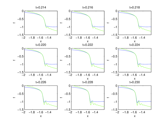
Figure 10. The blue line is the solution of the CH equation for the initial data $u_{0}(x)=-1/\cosh^{2}x$ and $\epsilon=10^{-2}$, and the green line is the corresponding multiscale solution. The plots are given for different times near the point of gradient catastrophe $(x_{c},t_{c})$ of the Hopf solution. Here $x_{c}\simeq-1.524$, $t_{c}\simeq 0.216$.

The same qualitative behavior can also be observed for smaller $\epsilon$ in Fig. 11, though the quality of the approximation increases as expected on the respective scales. Note that we plotted in Fig. 10 and Fig. 11 the CH solution instead of the function $\tilde{u}$, since there are no visible differences between the two for the used values of $\epsilon$.

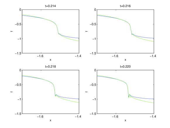
Figure 11. The blue line is the solution of the CH equation for the initial data $u_{0}(x)=-1/\cosh^{2}x$ and $\epsilon=10^{-3}$, and the green line is the corresponding multiscale solution. The plots are given for different times near the point of gradient catastrophe $(x_{c},t_{c})$ of the Hopf solution.

Appendix A Numerical solution of the fourth order equation

We are interested in the numerical solution of the fourth order ordinary equation (ODE) (1.5) with the asymptotic conditions (1.6). Numerically we will consider the equation on the finite interval $[X_{l},X_{r}]$, typically $X_{r}=-X_{l}=100$. In the exterior of this interval the solution to the equation (1.5) is obtained in the form of a Laurent expansion of $F$ around infinity in terms of $Y=X^{1/3}$,

(A.1) $$U=Y+\sum_{n=1}^{\infty}\frac{(-1)^{n}a_{n}}{Y^{n}}.$$

We find the non-zero coefficients (not-given coefficients vanish) $a_{1}=2T,$ $a_{5}=-8T^{3}/3$, $a_{6}=1/18$, $a_{7}=16T^{4}/3$, $a_{8}=-5T/27$, $a_{10}=14T^{2}/27$, $a_{11}=-256T^{6}/9$, $a_{12}=16T^{3}/3$, $a_{13}=640T^{7}/9-7/108$, …This expansion also determines the boundary values we impose at $X_{l}$, $X_{r}$ for $U$ and $U_{X}$.

The solution in the interval $[X_{l},X_{r}]$ is numerically obtained with a finite difference code based on a collocation method. The code bvp4c distributed with Matlab, see [19] for details, uses cubic polynomials in between the collocation points. The ODE (1.5) is rewritten in the form of a first order system. With some initial guess (we use $U_{0}=-X^{1/3}$ as the initial guess), the differential equation is solved iteratively by linearization. The collocation points (we use up to 10000) are dynamically adjusted during the iteration. The iteration is stopped when the equation is satisfied at the collocation points with a prescribed relative accuracy, typically $10^{-6}$. The values of $U$ in between the collocation points are obtained via the cubic polynomials in terms of which the solution has been constructed. This interpolation leads to a loss in accuracy of roughly one order of magnitude with respect to the precision at the collocation points. To test this we determine the numerical solution via bvp4c for (1.5) on Chebychev collocation points and check the accuracy with which (1.5) is satisfied via Chebychev differentiation, see e.g. [22]. We are interested here in values of $|T|<1$ and $|X|<10$. It is found that the numerical solution with a relative tolerance of $10^{-6}$ on the collocation points satisfies the ODE to the order of better than $10^{-4}$, see Fig. 12 where we show the residual $\Delta$ by plugging the numerical solution into the differential equation. It is straight forward to obtain higher accuracy by requiring a lower value for the relative tolerance, but we will only need an accuracy of the solution of the order of $10^{-4}$ here.

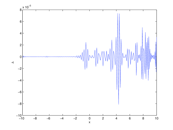
Figure 12. Residual of the numerical solution to the ODE (1.5) for $t=0.23$. The derivatives are computed with Chebychev differentiation.

References

- [1] A. Bressan, One dimensional hyperbolic systems of conservation laws, Current developments in mathematics (2002), 1–37, Int. Press, Somerville, MA, 2003.
- [2] E. Brézin, E. Marinari and G. Parisi, A nonperturbative ambiguity free solution of a string model, Phys. Lett. B, 242 (1990), no. 1, 35–38.
- [3] R. Camassa and D. D. Holm, An integrable shallow water equation with peaked solitons, Phys. Rev. Lett. 71 (1993), 1661-1664.
- [4] T. Claeys and M. Vanlessen, The existence of a real pole-free solution of the fourth order analogue of the Painleve I equation, Preprint:http://xxx.lanl.gov/math-ph/0604046.
- [5] T. Claeys and M. Vanlessen, Universality of a double scaling limit near singular edge points in random matrix models, Preprint:http://xxx.lanl.gov/math-ph/0607043.
- [6] P. Deift, and X. Zhou, A steepest descent method for oscillatory Riemann-Hilbert problems. Asymptotics for the MKdV equation, Ann. of Math. (2), 137, (1993), 295–368.
- [7] P. Deift, S. Venakides, and X. Zhou, New result in small dispersion KdV by an extension of the steepest descent method for Riemann-Hilbert problems, IMRN 6, (1997), 285-299.
- [8] P. Deift, T. Kriecherbauer, K. T.-R. McLaughlin, S. Venakides, and X. Zhou, Uniform asymptotics for polynomials orthogonal with respect to varying exponential weights and applications to universality questions in random matrix theory, Comm. Pure Appl. Math. 52 (1999), no. 11, 1335–1425.
- [9] B. Dubrovin and S. P. Novikov, A periodic problem for the Korteweg-de Vries and Sturm-Liouville equations. Their connection with algebraic geometry. Dokl. Akad. Nauk SSSR bf 219, (1974), 531–534.
- [10] B. Dubrovin, On Hamiltonian Perturbations of Hyperbolic Systems of Conservation Laws, II: Universality of Critical Behaviour, Comm. Math. Phys., 267 (2006), 117.
- [11] B. Dubrovin and Y. Zhang, Normal forms of hierarchies of integrable PDEs, Frobenius manifolds and Gromov - Witten invariants, Preprint:http://xxx.lanl.gov/math.DG/0108160.
- [12] A. S. Fokas, On a class of physically important integrable equations, Physica D 87 (1995), 145–150.
- [13] T. Grava and C. Klein, Numerical solution of the small dispersion limit of Korteweg de Vries and Whitham equations, to appear in Comm. Pure Appl. Math. (2006).
- [14] A. G. Gurevich and L. P. Pitaevskii, Non stationary structure of a collisionless shock waves, JEPT Letters 17 (1973), 193-195.
- [15] A. Its and V. B. Matveev, Hill operators with a finite number of lacunae, (Russian) , Funkcional. Anal. i Priložen. 7 (1975), no. 1, 69–70.
- [16] S. Kamvissis, K.D.T.-R McLaughlin, P. Miller, Semiclassical soliton ensembles for the focusing nonlinear Schrödinger equation, Annals of Mathematics Studies, 154, Princeton University Press, Princeton, NJ, 2003.
- [17] C. Klein, Fourth order time-stepping for low dispersion Korteweg-de Vries and nonlinear Schrödinger equation, preprint (2006).
- [18] P. D. Lax and C. D. Levermore, The small dispersion limit of the Korteweg de Vries equation, I,II,III, Comm. Pure Appl. Math. 36 (1983), 253-290, 571-593, 809-830.
-
[19]
L. F. Shampine, M. W. Reichelt and J. Kierzenka,
Solving Boundary Value Problems for Ordinary Differential
Equations in MATLAB with bvp4c, available at
http://www.mathworks.com/bvp_tutorial - [20] Fei-Ran Tian, Oscillations of the zero dispersion limit of the Korteweg de Vries equations, Comm. Pure App. Math. 46 (1993) 1093-1129.
- [21] A. Tovbis, S. Venakides, X. Zhou,On semiclassical (zero dispersion limit) solutions of the focusing nonlinear Schrödinger equation. Comm. Pure Appl. Math. 57 (2004), no. 7, 877–985.
- [22] L. N. Trefethen, Spectral Methods in MATLAB, SIAM, Philadelphia, PA, 2000.
- [23] S. Venakides, The Korteweg de Vries equations with small dispersion: higher order Lax-Levermore theory, Comm. Pure Appl. Math. 43 (1990), 335-361.
- [24] G. B. Whitham, Linear and nonlinear waves, J.Wiley, New York, 1974.