$H=xp$ with interaction and the Riemann zeros

Abstract

Starting from a quantized version of the classical Hamiltonian $H=xp$, we add a non local interaction which depends on two potentials. The model is solved exactly in terms of a Jost like function which is analytic in the complex upper half plane. This function vanishes, either on the real axis, corresponding to bound states, or below it, corresponding to resonances. We find potentials for which the resonances converge asymptotically toward the average position of the Riemann zeros. These potentials realize, at the quantum level, the semiclassical regularization of $H=xp$ proposed by Berry and Keating. Furthermore, a linear superposition of them, obtained by the action of integer dilations, yields a Jost function whose real part vanishes at the Riemann zeros and whose imaginary part resembles the one of the zeta function. Our results suggest the existence of a quantum mechanical model where the Riemann zeros would make a point like spectrum embbeded in the continuum. The associated spectral interpretation would resolve the emission/absortion debate between Berry-Keating and Connes. Finally, we indicate how our results can be extended to the Dirichlet L-functions constructed with real characters.

I Introduction

The Riemann hypothesis is considered the most important problem in Analytic Number Theory Edwards ; Titchmarsh2 ; Bombieri ; Sarnak ; Conrey . It states that the non trivial zeros of the classical zeta function have real part equal to $1/2$. Hilbert and Pólya suggested long ago that the RH can be proved if one finds a self-adjoint linear operator whose eigenvalues are the Riemann zeros Watkins ; Rosu ; Elizalde . The first indication of the adecuacy of this conjecture was probably the work by Selberg in the 1950s, who found a remarkable duality between the eigenvalues of the Laplacian acting on Riemann surfaces of constant negative curvature and the length spectrum of their geodesics Selberg . Selberg trace formula, which establishes that link, strongly resembles Riemann explicit formula. Another important hint came in 1973 from Montgomery’s work who, assuming the RH, showed that the Riemann zeros are distributed according to the Gaussian Unitary Ensemble statistics of random matrix models Mont . Montgomery’s results, were confirmed by the impressive numerical findings obtained by Odlyzko in the 1980’s Odl . The next step in this direction was put forward by Berry who proposed the Quantum Chaos conjecture, according to which the Riemann zeros are the spectrum of a Hamiltonian obtained by quantization of a classical chaotic Hamiltonian, whose periodic orbits are labelled by the prime numbers B-chaos . This suggestion was based on analogies between fluctuation formulae in Number Theory and Quantum Chaos Gutzwiller . Another interesting approaches to the RH are based on Statistical Mechanical ideas Julia ; BC . The prime numbers has also been considered from a quantum mechanical viewpoint Mussardo .

Up to date, it is not known a Hamiltonian accomplishing the Hilbert-Pólya conjecture. Along these lines, Berry and Keating suggested in 1999 that the 1d classical Hamiltonian $H=xp$ is related to the Riemann zeros BK1 ; BK2 . This suggestion was based on a heuristic and semiclassical analysis which yields, rather surprisingly, the average number of Riemann zeros up to a given height. Unfortunately, this encouraging result does not have a quantum counterpart. More explicitely, it is not known a quantization of $H=xp$ yielding the average, or exact, position of the Riemann zeros as eigenvalues. The Berry-Keating papers were inspired by an earlier one from Connes who tried to prove the RH in terms of the mathematical structures known as adeles and p-adic numbers Connes . In order to illustrate the adelic approach, Connes introduced the Hamiltonian $H=xp$, using a different semiclassical regularization. In Connes’s approach the Riemann zeros appear as missing spectral lines in a continuum, which does not conform to the Berry-Keating’s approach where the Riemann zeros appear as discrete spectra. Both approaches are heuristic and semiclassical, therefore the apparent contradiction between them cannot be resolved until one derives a consistent quantum theory of $H=xp$, and its possible extensions.

In reference JSTAT we proposed a quantization of $H=xp$ using an unexpected connection of this model to the one-body version of the so called Russian doll BCS model of superconductivity RD1 ; RD2 ; links . The latter model was, in turn, motivated by previous papers on the Renormalization Group with limit cycles GW ; BLflow ; nuclear (see also fewbody ; morozov ). The relation between $H=xp$ and the Russian doll (RD) model is as follows. An eigenstate, with energy $E$, of a quantum version of the classical Hamiltonian $H=xp$, corresponds to a zero energy eigenstate of the RD Hamiltonian, where $E$ becomes a coupling constant. Since the RD model is exactly solvable links , so it is the $H=xp$ model. The spectrum obtained in this way was shown to agree with Connes’s picture of a continuum of eigenstates JSTAT . We also obtained the smooth part of the Riemann formula for the zeros, however this fact cannot be interpreted as missing states but rather as a blueshift of energy levels. A point like spectrum associated to the Riemann zeros was completely absent in this quantization of $H=xp$. The final conclusion of JSTAT was the necessity to go beyond the $H=xp$ model, in order to realize an spectral interpretation of the Riemann zeros. Some proposals were already made in that reference but the corresponding models could not be solved exactly.

The cyclic Renormalization Group, and its realization in the field theory models of references LRS1 ; LRS2 ; LS , is at the origin of LeClair’s approach to the RH Andre . In this reference the zeta function on the critical strip is related to the quantum statistical mechanics of non-relativistic, interacting fermionic gases in 1d with a quasi-periodic two-body potential. This quasi-periodicity is reminiscent of the zero temperature cyclic RG of the quantum mechanical Hamiltonian of JSTAT , but the general framework of both works is different. The cyclic RG underlies several of the results of the present paper, but we shall not deal with it in the rest of the paper.

The organization of the paper is as follows. In section II we review the Berry-Keating and Connes semiclassical approaches to $H=xp$. In section III we quantize this Hamiltonian, finding its self-adjoint extensions and their relation to the semiclassical approaches of section II. We also study the inverse Hamiltonian $1/(xp)$ and its connection to the Russian doll model. In section IV we add an interaction to a quantized version of $H=1/(xp)$, and solve the general model exactly, in terms of a Jost like function. Section V is devoted to the analiticity properties of this Jost function. In section VI we study the potentials which exhibit some relation to the Riemann zeros.

II Semiclassical approach

The classical Berry-Keating-Connes (BKC) Hamiltonian BK1 ; BK2 ; Connes

$$H^{\rm cl}_{0}=x\;p,$$ (1)

has classical trayectories given by the hyperbolas (see fig.1a)

$$x(t)=x_{0}\;e^{t},\quad p(t)=p_{0}\;e^{-t}.$$ (2)

The dynamics is unbounded, so one should not expect a discrete spectrum at the quantum level. In 1999 Berry and Keating on the one hand BK1 ; BK2 , and Connes on the other Connes , introduced two different types of regularizations of the model and made a semiclassical counting of states. Berry and Keating proposed the Planck cell in phase space: $|x|>l_{x}$ and $|p|>l_{p}$, with $l_{x}\,l_{p}=2\pi\hbar$, while Connes choosed $|x|<\Lambda$ and $|p|<\Lambda$, where $\Lambda$ is a cutoff. In reference JSTAT we considered a third regularization which combines the previous ones involving the position $x$, namely $l_{x}<x<\Lambda$, making no assumption for the momenta $p$. The number, ${\cal N}(E)$, of semiclassical states with an energy lying between $0$ and $E$ is given by

$${\cal N}(E)={A\over 2\pi\hbar},$$ (3)

where $A$ is the area of the allowed phase space region below the curve $E=x\;p$ (see figs.1b,1c,1d). Table 1 collects the values of ${\cal N}(E)$ for the three types of regularizations.

Type	Regularization	${\cal N}(E)$
BK	$|x|>l_{x},\;\;|p|>l_{p}$	${E\over 2\pi}\left(\log{E\over 2\pi}-1\right)+1$
C	$|x|<\Lambda,\;\;|p|<\Lambda$	${E\over\pi}\log\Lambda-{E\over 2\pi}\left(\log{E\over 2\pi}-1\right)$
S	$l_{x}<x<\Lambda$	${E\over 2\pi}\log{\Lambda\over l_{x}}$

Table 1.- Three different regularizations of $H=xp$ and the corresponding number of semiclassical states in units $\hbar=1$.

In the BK regularization, the number of semiclassical states agrees, quite remarkably, with the asymptotic limit of the smooth part of the formula giving the number of Riemann zeros whose imaginary part lies in the interval $(0,E)$,

$$\langle{\cal N}(E)\rangle\sim{E\over 2\pi}\left(\log{E\over 2\pi}-1\right)+{7\over 8}+\dots,\qquad E>>1.$$ (4)

The exact formula for the number of zeros, ${\cal N}_{R}(E)$, is due to Riemann, and contains also a fluctuation term which depends on the zeta function Edwards ,

$${\cal N}_{R}(E) = \langle{\cal N}(E)\rangle+N_{\rm fl}(E)$$ (5)

$$\langle{\cal N}(E)\rangle = {1\over\pi}\,{\rm Im}\log\Gamma\left({1\over 4}+{i\over 2}E\right)-{E\over 2\pi}\log\pi+1$$

$${\cal N}_{\rm fl}(E) = ={1\over\pi}{\rm Im}\log\zeta\left({1\over 2}+iE\right)$$

Figure 1: 1a) a classical trayectory (2). The regions in shadow are the allowed phase space of the semiclassical regularizations of $H=xp$ considered by: 1b) Berry and Keating, 1c) Connes and 1d) Sierra. The values of the associated areas are given in table 1.

Based on this result, and analogies between formulae in Number Theory and Quantum Chaos, Berry and Keating suggested the existence of a classical chaotic hamiltonian whose quantization would give rise to the zeros as point like spectra BK1 ; BK2 . They conjectured the properties of this classical Hamiltonian, which include the breaking of time reversal symmetry, which holds for (1), and the existence of primitive periodic orbits labelled by the prime numbers. However, up to now, there is no a concrete proposal realizing all these conditions.

On the other hand, Connes found that the number of semiclassical states diverges in the limit where the cutoff $\Lambda$ goes to infinity, and that there is a finite size correction given by minus the average position of the Riemann zeros (see table 1). This result led to the missing spectral interpretation of the Riemann zeros, according to which there is a continuum of eigenstates (represented by the term ${E\over\pi}\log\Lambda$ in ${\cal N}(E)$), where some of the states are missing, precisely the ones associated to the Riemann zeros. This interpretation, albeit appealing, has the trouble that the number of missing states changes linearly in $E$ after scaling the cutoff $\Lambda$, and thus it is regularization dependent. As in the BK case, the C-regularization is not supported by a quantum mechanical version of $H=xp$, although it serves to illustrate, in a simple example, the main ideas underlying the Connes’s adelic approach to the Riemann hypothesis.

Finally, in the S-regularization the number of semiclassical states diverges as ${E\over 2\pi}\log\Lambda/l_{x}$, suggesting a continuum spectrum, like in Connes’s approach. But there is no a finite size correction to that formula, and consequently the possible connection to the Riemann zeros is lost. The main advantage of this regularization is that the Hamiltonian (1) can be consistently quantized yielding a spectrum which coincides with the semiclassical result as we show below.

III Quantization of $x\,p$ and $1/(xp)$

III.1 The Hamiltonian $H_{0}=xp$

In this section we construct a self-adjoint operator $H_{0}$, associated to $H_{0}^{\rm cl}=x\,p$, which acts on the Hilbert space $L^{2}(a,b)$ of square integrable functions in the interval $(a,b)$. Assuming that $x\geq 0$, there are four possible intervals corresponding to the choices: $a=0,l_{x}$ and $b=\Lambda,\infty$, where $l_{x}$ and $\Lambda$ were introduced above (we shall take $l_{x}=1$ and $\Lambda=N>1$). Berry and Keating defined the quantum Hamiltonian $H_{0}$ as the normal ordered expression

$$H_{0}={1\over 2}(x\,p+p\,x),$$ (6)

where $p=-i\hbar\;d/dx$. If $x\geq 0$, eq.(6) is equivalent to

$$H_{0}=\sqrt{x}\,p\,\sqrt{x}=-i\hbar\sqrt{x}\,{d\over dx}\,\sqrt{x}.$$ (7)

This is a symmetric operator acting in a certain domain of the Hilbert space $L^{2}(a,b)$, if Galindo

$$\langle\psi|H_{0}\phi\rangle-\langle H_{0}\psi|\phi\rangle=i\hbar\left[a\psi^{*}(a)\phi(a)-b\psi^{*}(b)\phi(b)\right]=0,$$ (8)

which is satisfied if both $\psi(x)$ and $\phi(x)$ vanish at the points $a,b$. By a theorem due to von Neumman, the symmetric operator $H_{0}$ is also self-adjoint if its deficiency indices $n_{\pm}$ are equal Neumann . These indices counts the number of solutions of the eq.

$$H_{0}^{\dagger}\,\psi_{\pm}=\pm i\hbar\,\lambda\,\psi_{\pm},$$ (9)

belonging to the domain of $H_{0}^{\dagger}$ ($\lambda>0$). If $n=n_{+}=n_{-}>0$, there are infinitely many self-adjoint extensions of $H_{0}$ parameterized by a unitary $n\times n$ matrix. The solutions of eq.(9) are

$$\psi_{\pm}(x)=Cx^{-1/2\mp\lambda},$$ (10)

whose norm in the interval $(a,b)$ is,

$$\langle\psi_{\pm}|\psi_{\pm}\rangle=\pm{C^{2}\over 2\lambda}(a^{\mp 2\lambda}-b^{\mp 2\lambda}).$$ (11)

The deficiency indices corresponding to the four intervals considered above are collected in table 2.

Type	$(a,b)$	$(n_{+},n_{-})$	Self-adjoint
BK	$(1,\infty)$	$(1,0)$	-
C	$(0,N)$	$(0,1)$	-
S	$(1,N)$	$(1,1)$	$\surd$
T	$(0,\infty)$	$(0,0)$	$\surd$

Table 2.- Deficiency indices of $H_{0}$. The corresponding intervals are associated to the semiclassical regularizations of section II (i.e. BK, C, S). The last one, T, describes the case with no constraints on $x$ except positivity (i.e. $x>0)$.

The von Neumann theorem implies that the operator $H_{0}$ is essentially self-adjoint on the half line $\vbox{\hbox{\upright\hbox to0.0pt{I\hss}\kern 1.7ptR}}_{+}=(0,\infty)$. This case was recently studied by Twamley and Milburn, who defined a quantum Mellin transform using the eigenstates of $H_{0}$ Twamley .

On the other hand, in the interval $(1,N)$ the operator $H_{0}$ admits infinitely many self-adjoint extensions parameterized by a phase $e^{i\theta}$. This phase determines the boundary conditions of the functions belonging to the self-adjoint domain

$${\cal D}(H_{0,\theta})=\left\{\psi,H_{0}\psi\in L^{2}(1,N),\;\;e^{i\theta}\psi(1)=\sqrt{N}\psi(N)\right\}.$$ (12)

The eigenfunctions of $H_{0}$,

$$H_{0}\;\psi_{E}=E\;\psi_{E},$$ (13)

are given by BK1

$$\psi_{E}(x)={C\over x^{1/2-iE\hbar}},\qquad E\in\vbox{\hbox{\upright\hbox to0.0pt{I\hss}\kern 1.7ptR}},$$ (14)

where $C$ is a normalization constant. In the half line $\vbox{\hbox{\upright\hbox to0.0pt{I\hss}\kern 1.7ptR}}_{+}$ there are no further restrictions on $E$, hence the spectrum of $H_{0}$ is continuous and covers the whole real line IR . In this case the normalization constant in (14) is choosen as $C=1/\sqrt{2\pi\hbar}$ which guarantees the standard normalization

$$\langle\psi_{E}|\psi_{E^{\prime}}\rangle=C^{2}\int_{0}^{\infty}{dx\over x}x^{-i(E-E^{\prime})/\hbar}=\delta(E-E^{\prime}).$$ (15)

In the case where $H_{0}$ is defined in the interval $(1,N)$, the boundary condition (12) yields the quantization condition for $E$, namely

$$N^{iE/\hbar}=e^{i\theta}\Longrightarrow E_{n}={2\pi\hbar\over\log N}\left(n+{\theta\over 2\pi}\right),\;\;n\in\vbox{\hbox{\upright\hbox to0.0pt{I\hss}\kern 1.7ptN}}.$$ (16)

Hence the spectrum of $H_{0}$ is discrete, with a level spacing decreasing for large values of $N$. The normalization constant of the wave function is now $C={1\over\sqrt{\log N}}$ which gives,

$$\langle\psi_{E_{n}}|\psi_{E_{n^{\prime}}}\rangle=C^{2}\int_{1}^{N}{dx\over x}x^{-i(E_{n}-E_{n^{\prime}})/\hbar}=\delta_{n,n^{\prime}}.$$ (17)

The spectrum (16) agrees with the semiclassical result given in table 1 for the S-regularization (recall that $l_{x}=1,\Lambda=N,\hbar=1)$.

The existence of only two self-adjoint extensions of the operator $H_{0}$, in the positive real axis, should not be surprising, since they are intimately related to those of the momenta operator $P=-i\hbar{d\over dq}$, where $q=\log x$. Indeed, the $P$ operator defined on IR , admits only two self-adjoint extensions in the $q$-intervals: $(-\infty,\infty)$ and $(a,b)$ ($a,b$ finite), which correspond to the $x$-intervals: $(0,\infty)$ and $(\log a,\log b)$, respectively. Under this mapping, the wave function (14) corresponds to the plane wave $e^{iqE}$, where $x^{1/2}$ is a measure factor. The spectrum of $H_{0}$ can therefore be understood in terms of the familiar spectrum of $P$.

Returning to (16), for the particular case where $\theta=\pi$, one observes that the energy spectrum is symmetric around zero, i.e. if $E_{n}$ is an eigenenergy so is $-E_{n}$. This result was obtained in reference JSTAT working with the inverse Hamiltonian $1/H_{0}$. We shall next review that construction since it will be important in the sequel.

III.2 The inverse Hamiltonian $1/H_{0}$

First, we start from the expression (7) and take the formal inverse, i.e. $H_{0}^{-1}=x^{-1/2}\,p^{-1}\,x^{-1/2}$. The operator $p^{-1}$ is the one dimensional Green function with matrix elements $\langle x|p^{-1}|x^{\prime}\rangle={i\over 2\hbar}\;{\rm sign}(x-x^{\prime})$, where ${\rm sign}(x-x^{\prime})$ is the sign function. The operator $H_{0}^{-1}$ is defined in the interval $(1,N)$ by the continuous matrix,

$$H_{0}^{-1}(x,x^{\prime})={i\over 2\hbar}{{\rm sign}(x-x^{\prime})\over\sqrt{x\,x^{\prime}}},\qquad 1\leq x,x^{\prime}\leq N.$$ (18)

Its spectrum is found solving the Schrödinger equation

$${i\over 2\hbar}\int_{1}^{N}dx^{\prime}\;{{\rm sign}(x-x^{\prime})\over\sqrt{x\,x^{\prime}}}\;\psi(x^{\prime})=E^{-1}\;\psi(x),$$ (19)

for the eigenvalue $E^{-1}$, which must not be singular for $H_{0}^{-1}$ to be invertible. Define a new wave function

$$\phi(x)={\psi(x)\over\sqrt{x}},$$ (20)

which satisfies

$${iE\over 2\hbar}\int_{1}^{N}dx^{\prime}\;{\rm sign}(x-x^{\prime})\;\phi(x^{\prime})=x\;\phi(x).$$ (21)

Taking the derivative with respect to $x$ yields

$$x{d\over dx}\phi(x)=\left(1-{iE\over\hbar}\right)\phi(x),$$ (22)

which is solved by

$$\phi(x)={C\over x^{1-iE/\hbar}}\Rightarrow\psi(x)={C\over x^{1/2-iE/\hbar}},$$ (23)

with $C=1/\sqrt{\log N}$ as in (17). Eq. (23) fixes the functional form of $\psi(x)$. To find the spectrum we impose (21) at one point, say $x=1$, obtaining,

$$N^{iE/\hbar}=-1\Longrightarrow E_{n}={2\pi\hbar\over\log N}(n+{1\over 2}),\qquad n\in\vbox{\hbox{\upright\hbox to0.0pt{I\hss}\kern 1.7ptN}}$$ (24)

This spectrum coincides with (16) for $\theta=\pi$, so that the eigenenergies come in pairs $\{E_{n},-E_{n}\}$, as corresponds to an hermitean antisymmetric operator. Including a BCS coupling in (18), related to $\theta$, yields the spectrum (16) JSTAT .

In summary, we have constructed in this section a quantum version of the classical Hamiltonian $xp$, as well as its inverse $1/(xp)$, which agree with the semiclassical regularization $l_{x}<x<\Lambda$. Both, the semiclassical regularization, and the associated quantization, shows no trace of the Riemann zeros, which suggests that a possible connection to them requires to go beyond the $xp$ model. In the next section we shall take a further step in that direction.

IV $H_{0}=x\;p$ with interactions

IV.1 Definition of the Hamiltonian

The standard way to add an interaction to a free Hamiltonian $H_{0}$ is to perturb it by a potential term, i.e.

$$H=H_{0}+V.$$ (25)

Instead of starting from the Hamiltonian $H_{0}$ (6) we shall perturb the inverse Hamiltonian $1/H_{0}$ (18)

$${1\over H}={1\over H_{0}}+V^{\prime}$$ (26)

so that $H$ depends non linearly on $V^{\prime}$. We have found more convenient to work with (26), rather than with (25) but, of course, the two formulations must be related (we leave this issue for a later publication).

The interacting Hamiltonian $1/H$ that we shall consider is given by,

$$H^{-1}_{2}(x,x^{\prime})={i\over 2\hbar}{{\rm sign}(x-x^{\prime})+a(x)b(x^{\prime})-b(x)a(x^{\prime})\over\sqrt{\varepsilon(x)\varepsilon(x^{\prime})}},$$ (27)

where $a(x)$ and $b(x)$ are two real functions defined in the interval $x\in(1,N)$, and $\varepsilon(x)$ is a positive and monotonically increasing function. The BKC model corresponds to the choice $\varepsilon(x)=x$, but it is equally easy to work with generic functions $\varepsilon(x)$, which also links the present model to the RD model, where $\varepsilon(x)$ gives the energy levels of electrons pairs.

$H^{-1}_{2}$ is an hermitean antisymmetric operator, and hence its spectrum is real and symmetric around zero. We shall assume, for the time being, that $H^{-1}_{2}$ is invertible, a condition which depends on the potentials $a(x)$ and $b(x)$. If one of the potentials is constant, say $b(x)=1$, then (27) becomes

$$H^{-1}_{1}(x,x^{\prime})={i\over 2\hbar}{{\rm sign}(x-x^{\prime})+a(x)-a(x^{\prime})\over\sqrt{\varepsilon(x)\varepsilon(x^{\prime})}}.$$ (28)

We shall denote ${\cal M}_{2}$ (resp. ${\cal M}_{1}$) the model with Hamiltonian (27) (reps. (28)). These two models share many properties but they differ in some important instances. For example, (27) is invariant under the transformation

$$\left(\begin{array}[]{cc}a(x)\\ b(x)\\ \end{array}\right)\rightarrow\left(\begin{array}[]{cc}\alpha&\beta\\ \gamma&\delta\\ \end{array}\right)\left(\begin{array}[]{cc}a(x)\\ b(x)\\ \end{array}\right),\qquad\forall x\in(1,N),$$ (29)

where the $2\times 2$ matrix is an element of the $Sl(2,\vbox{\hbox{\upright\hbox to0.0pt{I\hss}\kern 1.7ptR}})$ group,

$$\left(\begin{array}[]{cc}\alpha&\beta\\ \gamma&\delta\\ \end{array}\right)\in Sl(2,\vbox{\hbox{\upright\hbox to0.0pt{I\hss}\kern 1.7ptR}})\Leftrightarrow\alpha,\beta,\gamma,\delta\in\vbox{\hbox{\upright\hbox to0.0pt{I\hss}\kern 1.7ptR}},\;\;\alpha\delta-\beta\gamma=1.$$ (30)

while (28) is invariant under the translations,

$$a(x)\rightarrow a(x)+\alpha,\qquad\alpha\in\vbox{\hbox{\upright\hbox to0.0pt{I\hss}\kern 1.7ptR}}.$$ (31)

Naturally, the spectra of $H_{1,2}$ must be invariant under the corresponding symmetry transformations. The Hamiltonian (27) can also be written as

$$H_{2}^{-1}(x,x^{\prime})=H_{0}^{-1}(x,x^{\prime})+{i\over 2\hbar}\left[\psi_{a}(x)\psi_{b}(x^{\prime})-\psi_{b}(x)\psi_{a}(x^{\prime})\right],$$ (32)

where

$$\psi_{a}(x)={a(x)\over\sqrt{\varepsilon(x)}},\quad\psi_{b}(x)={b(x)\over\sqrt{\varepsilon(x)}}.$$ (33)

This means that the interaction is given by a sort of proyection operator formed by the states $\psi_{a,b}$. In section VI we show that a particular choice of $\psi_{a,b}$ provides a quantum version of the BK semiclassical regularization conditions. The Hamiltonians (27) and (28) admit a discrete version analogue to the one considered in JSTAT . The results we shall derive in the coming sections are also valid in this case. Furthermore, the connection with the RD model provides an interesting many-body generalization which will studied in a separate work.

IV.2 Solution of the Schrödinger equation

The Schrödinger equation associated to (27) reads (in units of $\hbar=1$),

$${i\over 2}\int_{1}^{N}dx^{\prime}\;{{\rm sign}(x-x^{\prime})+a(x)b(x^{\prime})-b(x)a(x^{\prime})\over\sqrt{\varepsilon(x)\varepsilon(x^{\prime})}}=E^{-1}\psi(x)$$ (34)

which for the wave function

$$\phi(x)={\psi(x)\over\sqrt{\varepsilon(x)}},$$ (35)

becomes

$$\varepsilon(x)\;\phi(x)=$$ (36)

$${iE\over 2}\int_{1}^{N}dx^{\prime}\;\left({\rm sign}(x-x^{\prime})+a(x)b(x^{\prime})-b(x)a(x^{\prime})\right)\phi(x^{\prime}).$$

This equation is the basis for the relation between the BKC and the RD models. Indeed, defining the RD Hamiltonian

$$H_{RD_{2}}(x,x^{\prime})=$$ (37)

$$\varepsilon(x)\delta(x-x^{\prime})-{ih_{D}\over 2}\left({\rm sign}(x-x^{\prime})+a(x)b(x^{\prime})-b(x)a(x^{\prime})\right),$$

we see that (36) becomes the eigenequation of a zero energy eigenstate $\phi(x)$,

$$H_{2}\;|\psi\rangle=E|\psi\rangle\Longleftrightarrow H_{RD_{2}}\;|\phi\rangle=0,$$ (38)

provided the coupling $h_{D}$ is related to the energy $E$ by

$$h_{D}=E.$$ (39)

Eqs.(38) and (39) establish a one-to-one correspondence between the energy spectrum of the Hamiltonian $H_{2}$, and the coupling constant spectrum of zero energy states of the Hamiltonian $H_{RD_{2}}$. In this regard, we shall mention the work by Khuri khuri , based on a suggestion by Chadan Chadan , where the Riemann zeros are related to the “coupling constant spectrum” of zero energy, s-wave, scattering problem for repulsive potentials in standard Quantum Mechanics. In that model the coupling constant, $\lambda$, is related to the zeros, $s_{n}=1/2+i\gamma_{n}$, by the quadratic equation $\lambda=s(s-1)$. In our model however, the relation between the coupling constant, $h_{RD}$, and the energy $E$ is linear (eq.(39)), which is due to the fact that $H_{0}$ depends linearly on $d/dx$, while in standard QM the kinetic term depends quadratically.

We shall next solve eq.(36) for generic values of $a(x)$ and $b(x)$. Later on, we shall impose additional constraints on these functions so that the model makes sense in the limit $N\rightarrow\infty$. First of all, let us write (36) as

$${iE\over 2}\int_{1}^{N}dx^{\prime}\;{\rm sign}(x-x^{\prime})\;\phi(x^{\prime})+a(x)B-b(x)A=\varepsilon(x)\;\phi(x),$$ (40)

where

$$A={iE\over 2}\int_{1}^{N}dx\;a(x)\;\phi(x),\;B={iE\over 2}\int_{1}^{N}dx\;b(x)\;\phi(x).\qquad$$ (41)

Eq.(40) is equivalent to

$$iE\phi(x)+{da\over dx}B-{db\over dx}A={d\over dx}\left(\varepsilon(x)\;\phi(x)\right)$$ (42)

$$-{iE\over 2}\int_{1}^{N}dx\;\phi(x)+a_{1}B-b_{1}A=\varepsilon(1)\;\phi(1),$$ (43)

which are obtained from (40) by taking the derivative with respect to $x$, and setting $x=1$ with $a_{1}=a(x=1)$ and $b_{1}=b(x=1)$. Define the variable $q$

$$q=\int_{1}^{x}{dx^{\prime}\over\varepsilon(x^{\prime})},$$ (44)

such that

$$q\in(0,L_{N}),\qquad L_{N}=\int_{1}^{N}{dx^{\prime}\over\varepsilon(x^{\prime})}.$$ (45)

In the BKC model, i.e. $\varepsilon(x)=x$, one gets $q=\log x$ and $L_{N}=\log N$. For more general choices of $\varepsilon(x)$ we shall assume that $L_{N}\rightarrow\infty$ when $N\rightarrow\infty$. In terms of the new function

$${\widetilde{\phi}}(x)=\varepsilon(x)\;\phi(x),$$ (46)

eq.(42) turns into

$$\left({d\over dq}-iE\right){\widetilde{\phi}}(q)={da\over dq}B-{db\over dq}A,$$ (47)

where $a,b$ and ${\widetilde{\phi}}$ are regarded as functions of $q$. If $a$ and $b$ are zero, the solution of (47) is the plane wave $Ce^{iEq}$, with $C$ a constant. Otherwise, $C$ depends on $q$ and satisfies

$${dC\over dq}=e^{-iEq}\left({da\over dq}B-{db\over dq}A\right),$$ (48)

whose solution is

$$C(q)=C+\int_{0}^{q}dq^{\prime}\,e^{-iEq^{\prime}}\left({da\over dq^{\prime}}B-{db\over dq^{\prime}}A\right),$$ (49)

where $C$ is an integration constant. This equation fixes the functional form of ${\widetilde{\phi}}(q)$, namely

$${\widetilde{\phi}}(q)=Ce^{iEq}+e^{iEq}\int_{0}^{q}dq^{\prime}e^{-iEq^{\prime}}\left({da\over dq^{\prime}}B-{db\over dq^{\prime}}A\right),$$ (50)

and in turn of $\psi(x)$ by means of (35) and (46),

$$\psi(q)={e^{iqE}\over\sqrt{\varepsilon(q)}}\left[C+\int_{0}^{q}dq^{\prime}e^{-iEq^{\prime}}\left({da\over dq^{\prime}}B-{db\over dq^{\prime}}A\right)\right].$$ (51)

For $\varepsilon(x)=x$, eq.(51) becomes

$$\psi(x)={1\over x^{1/2-iE}}\left[C+\int_{1}^{x}dx^{\prime}x^{\prime-iE}\left({da\over dx^{\prime}}B-{db\over dx^{\prime}}A\right)\right].$$ (52)

The term proportional to $C$ in (52) coincides with (14). The integration constants $A,B$ and $C$ are related by eqs.(41) and (43),

$$A = {iE\over 2}\int_{0}^{L_{N}}dq\;a(q)\;{\widetilde{\phi}}(q),$$

$$B = {iE\over 2}\int_{0}^{L_{N}}dq\;b(q)\;{\widetilde{\phi}}(q),$$ (53)

$$C = -{iE\over 2}\int_{0}^{L_{N}}dq\;{\widetilde{\phi}}(q)+a_{1}B-b_{1}A.$$

Plugging (50) into (53) yields

$$(1+R_{a,b})\,A-R_{a,a}\,B-\;R_{a}\,C=0,$$

$$R_{b,b}\,A+(1-R_{b,a})\,B-R_{b}\,C=0,$$ (54)

$$(R_{1,b}-b_{1})\,A+(-R_{1,a}+a_{1})\,B-(R_{1}+1)\,C=0,$$

where

$$R_{f}(E) = {iE\over 2}\int_{0}^{L_{N}}dq\;f(q)\;e^{iEq},$$ (55)

$$R_{f,g}(E) = {iE\over 2}\int_{0}^{L_{N}}dq\;f(q)\;e^{iEq}\int_{0}^{q}dq^{\prime}\,{dg\over dq^{\prime}}e^{-iEq^{\prime}}.$$

We need in particular

$$R_{1}(E) = {1\over 2}(e^{iEL_{N}}-1),$$ (56)

$$R_{1,f}(E) = {1\over 2}f_{1}(1-e^{iEL_{N}})-e^{iEL_{N}}{\widetilde{R}}_{f}(E),$$

$$R_{f,g}(E) = S_{f,g}(E)-g_{1}\;R_{f}(E),$$

where

$$f_{1}=f(x=1),\;g_{1}=g(x=1),\;{\widetilde{R}}_{f}(E)=R_{f}(-E),$$ (57)

and

$$S_{f,g}(E) ={iE\over 2}\int_{0}^{L_{N}}dq\;f(q)\;g(q)$$

$$-{E^{2}\over 2}\int_{0}^{L_{N}}dq\;f(q)\;e^{iEq}\int_{0}^{q}dq^{\prime}\,g(q^{\prime})e^{-iEq^{\prime}}.$$

The latter integral plays an important role in the sequel. Eqs.(56) can be proved using the change in the order of integration,

$$\int_{0}^{L_{N}}dq\;\int_{0}^{q}dq^{\prime}=\int_{0}^{L_{N}}dq^{\prime}\;\int_{q^{\prime}}^{L_{N}}dq.$$ (59)

Plugging (56) into (54) leads to

$$(1+S_{a,b})\,A-S_{a,a}\,B-\;R_{a}\,(C+b_{1}A-a_{1}B)=0,$$

$$S_{b,b}\,A+(1-S_{b,a})\,B-R_{b}\,(C+b_{1}A-a_{1}B)=0,$$ (60)

$$2e^{iEL_{N}}({\widetilde{R}}_{b}\,A-{\widetilde{R}}_{a}B)+(e^{iEL_{N}}+1)(C+b_{1}A-a_{1}B)=0.$$

Observe that the term $C+b_{1}A-a_{1}B$ appears in all the equations. This parameter determines the asymptotic behaviour of the wave function at large values of $q$. Indeed, the value of $C(q)$ at $q=L_{N}$ (see eq.(49)) is given by

$$C_{N}\equiv C(q=L_{N})=C_{\infty}+e^{-iEL_{N}}(a_{N}\,B-b_{N}\,A),$$ (61)

where $a_{N}=a(x=N),b_{N}=b(x=N)$, and

$$C_{\infty}=C+A(b_{1}+2{\widetilde{R}}_{b})-B(a_{1}+2{\widetilde{R}}_{a}).$$ (62)

In the ${\cal M}_{2}$ model we shall impose

$$\lim_{N\rightarrow\infty}a_{N}=0,\quad\lim_{N\rightarrow\infty}b_{N}=0,\quad$$ (63)

while for the ${\cal M}_{1}$ model, only the vanishing of $a_{\infty}$ will be required, since $b(x)=1$. Under these conditions, $C_{N}$ converges asymptotically to $C_{\infty}$, as shown by (61). The latter parameter characterizes the asymptotic behaviour of the eigenfunctions,

$$\lim_{q>>1}\psi(q)\sim{e^{iqE}\over\sqrt{\varepsilon(q)}}\;C_{\infty}+\dots$$ (64)

If $C_{\infty}\neq 0$, the norm of $\psi(q)$ behaves as $\sqrt{L_{N}}$ when $N\rightarrow\infty$, and the wavefunction is delocalized, behaving asymptotically like the “plane waves” of the non interacting model. On the contrary, if $C_{\infty}=0$, the norm of $\psi(q)$ remains finite when $N\rightarrow\infty$ for potentials decaying sufficiently fast to infinity. An explicit expression for the norm of these localized states will be given at the end of section V. The localization of the wave function $\psi(q)$ is due to an “interference” effect, which can dissapear by an infinitesimal change of the potentials. This suggest that the bound states of the model, if any, must be embedded in the continuum spectrum, unlike ordinary QM where the discrete and continuum spectra usually belong to separated regions. There are however exceptions to this rule, as the class of von Neumann and Wigner oscillating potentials which have a unique bound state with positive energy embedded in the continuum Galindo ; neumann-wigner ; simon ; arai ; cruz .

Continuing with our analysis, let us combine the third equation of (60) and (62), obtaining

$$C+b_{1}A-a_{1}B=-e^{iEL_{N}}\,C_{\infty}.$$ (65)

Plugging (65) into (60), yields the following linear system of eqs.

$${\bf S}\;{\bf w}=0,\quad{\bf w}^{t}=(A,B,C_{\infty}),$$ (66)

where

$${\bf S}=\left(\begin{array}[]{ccc}1+S_{a,b}&-S_{a,a}&e^{iEL_{N}}R_{a}\\ S_{b,b}&1-S_{b,a}&e^{iEL_{N}}R_{b}\\ -2{\widetilde{R}}_{b}&2{\widetilde{R}}_{a}&e^{iEL_{N}}+1\end{array}\right).$$ (67)

The existence of non trivial solutions of (66) requires

$$\det{\bf S}={\cal F}(E)+{\widetilde{\cal F}}(E)\;e^{iEL_{N}}=0,$$ (68)

where

$${\cal F}(E)=1+S_{a,b}-S_{b,a}+S_{a,a}\;S_{b,b}-S_{a,b}\;S_{b,a},$$ (69)

and

$${\widetilde{\cal F}}(E) ={\cal F}(E)-2{\widetilde{R}}_{a}\left(R_{b}+R_{b}\;S_{a,b}-R_{a}\;S_{b,b}\right)$$ (70)

$$+2{\widetilde{R}}_{b}\left(R_{a}-R_{a}\;S_{b,a}+R_{b}\;S_{a,a}\right).$$

To simplify ${\widetilde{\cal F}}(E)$, we use the equation

$$S_{f,g}(E)+S_{g,f}(-E)=-2R_{f}(E)\;R_{g}(-E),$$ (71)

which implies

$${\widetilde{\cal F}}(E)={\cal F}(-E).$$ (72)

The final form of the eigenenergies equation is

$${\cal F}(E)+{\cal F}(-E)\;e^{iEL_{N}}=0.$$ (73)

Before we analyze in detail the possible solutions of (73) we shall make some comments.

• In the absence of interactions, i.e. $a(x)=b(x)=0$, one gets ${\cal F}(E)=1,\;\forall E$, and then eq.(73), for the case $\varepsilon(x)=x$, reproduces eq.(24).

• If $E$ is a solution of (73), so is $-E$ for generic potentials $a$ and $b$, including complex functions. This is a consequence of the antisymmetry of $H$.

• ${\cal F}(E)$ is invariant under the $SL(2,\vbox{\hbox{\upright\hbox to0.0pt{I\hss}\kern 1.7ptR}})$ transformation (29). In fact, the terms $S_{a,b}-S_{b,a}$ and $S_{a,a}\;S_{b,b}-S_{a,b}\;S_{b,a}$ are invariant separately.

• We shall assume that the integrals defining $R_{f}(E)$ and $S_{f,g}(E)$, converge for all values of $E$. At $E=0$ this implies

  $$R_{f}(0)=S_{f,g}(0)=0,\;\;f,g=a,b\Longrightarrow{\cal F}(0)=1,$$ (74)

  Hence $E=0$ is not a solution of eq.(73) and therefore the Hamiltonian $H^{-1}$ is non singular as assumed at the beginning of this section.

Returning to the solution of eq.(66), let us define the 3-component vectors,

$${\bf v}_{1} = (1+S_{a,b},\;-S_{a,a},\;e^{iEL_{N}}\,R_{a}),$$

$${\bf v}_{2} = (S_{b,b},\;1-S_{b,a},\;e^{iEL_{N}}\,R_{b}),$$ (75)

$${\bf v}_{3} = (-2{\widetilde{R}}_{b},\;2{\widetilde{R}}_{a},\;e^{iEL_{N}}+1),$$

which are the rows of the matrix ${\bf S}$, and are linearly dependent by (68). These vectors span a plane which can be characterized by its normal ${\bf n}$. The vector ${\bf w}$ that that solves (66), must be proportional to ${\bf n}$. If ${\bf v}_{1}$ and ${\bf v}_{2}$ are non collinear, we can choose

$${\bf w}={\bf v}_{1}\times{\bf v}_{2},\qquad{\bf v}_{1}\nparallel{\bf v}_{2},$$ (76)

where

$${\bf v}_{1}\times{\bf v}_{2}=$$ (77)

$$(-e^{iEL_{N}}(R_{b}S_{a,a}+R_{a}(1-S_{b,a})),$$

$$e^{iEL_{N}}(R_{a}S_{b,b}-R_{b}(1+S_{a,b})),\,{\cal F}).$$

We get in particular

$$C_{\infty}={\cal F}(E).$$ (78)

Hence the delocalized eigenstates, i.e. $C_{\infty}\neq 0$, satisfy that ${\cal F}(E)\neq 0$, while the localized ones, i.e. $C_{\infty}=0$, correspond to ${\cal F}(E)=0$.

Otherwise, if ${\bf v}_{1}$ and ${\bf v}_{2}$ are collinear, the vector ${\bf w}$ can be choosen as

$${\bf w}={\bf v}_{1}\times{\bf v}_{3},\qquad{\rm if}\;\;{\bf v}_{1}\parallel{\bf v}_{2},\;{\bf v}_{1}\nparallel{\bf v}_{3}.$$ (79)

This case is exceptional since it requires the vanishing of the functions giving ${\bf v}_{1}\times{\bf v}_{2}$. Another unlikely possibility is that the three vectors ${\bf v}_{i}$ are collinear, in which case the vector ${\bf w}$ must belong to the plane orthogonal to ${\bf v}_{1,2,3}$.

In summary, the most common situation we shall encounter is described by eqs.(76), so that the localized/delocalized nature of the eigenfunctions is fully characterized by the vanishing/non vanishing of ${\cal F}(E)$. The generic structure of the spectrum is depicted in figure 2 and table 3.

In so far we have not used the reality of the potentials $a$ and $b$, which guarantees the hermiticity of the Hamiltonian (27). If they are real functions, then ${\cal F}(E)$ is a complex hermitean function, i.e.

$$a(x),b(x)\in\vbox{\hbox{\upright\hbox to0.0pt{I\hss}\kern 1.7ptR}}\Longrightarrow{\cal F}^{*}(E)={\cal F}(-E^{*}).$$ (80)

This equation follows from the identity

$$S_{f,g}^{*}(E)=S_{f^{*},g^{*}}(-E^{*}).$$ (81)

If $E$ is real, eq.(80) implies that ${\cal F}^{*}(E)={\cal F}(-E)$ and hence the eigenvalue equation (73), for delocalized states, can be written as

$$e^{iEL_{N}}=-{{\cal F}(E)\over{\cal F}(E)^{*}},\qquad{\rm for}\;{\cal F}(E)\neq 0$$ (82)

The RHS of this equation describes the scattering phase shift produced by the interaction. For localized states, equation (82) becomes singular, but eq.(73) is automatically satisfied since ${\cal F}(E)={\cal F}(-E)=0$. All these results means that ${\cal F}(E)$ plays, in our model, the role of a Jost function which determines completely the scattering phases and bound states. However there are some important differences concerning their analytical properties that we shall discuss below.

Eigenstate	$C_{\infty}$	${\cal F}(E)$	Eigencondition
Delocalized	$\neq 0$	$\neq 0$	$e^{iEL_{N}}=-{{\cal F}(E)\over{\cal F}(E)^{*}}$
Localized	$=0$	$=0$	${\cal F}(E)=0$

Table 3.- Classification of eigenstates of the ${\cal M}_{2}$ model. For the ${\cal M}_{1}$ model, ${\cal F}(E)$ is replaced by ${\cal F}_{1}(E)$.

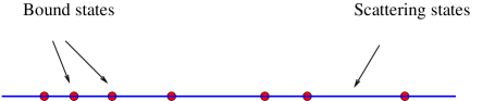
Figure 2: Pictorial representation of the spectrum of the model. The bound states are the points where ${\cal F}(E)=0$, which are embedded in a continuum of scattering states.

IV.3 Schrödinger equation for the ${\cal M}_{1}$ model

The diagonalization of the Hamiltonian $H_{1}$ (28) proceeds along the same steps as for $H_{2}$ with the suitable changes. The main difference is that the phase factor $e^{iEL_{N}}$ arises in several expressions which one needs to extract out and factorize conveniently. In particular, from (IV.2) one finds

$$S_{a,1}=R_{a},\;S_{1,a}=-e^{iEL_{N}}\;{\widetilde{R}}_{a},\;S_{1,1}={1\over 2}(e^{iEL_{N}}-1),$$

and then

$${\cal F}=1+R_{a}-{1\over 2}S_{a,a}+e^{iEL_{N}}\left({\widetilde{R}}_{a}+{1\over 2}S_{a,a}+R_{a}\;{\widetilde{R}}_{a}\right),$$ (83)

so that eq.(73) becomes

$${\cal F}_{1}(E)+e^{iEL_{N}}\,{\widetilde{\cal F}}_{1}(E)=0,$$ (84)

where

$${\cal F}_{1}(E)=1+2R_{a}-S_{a,a},\;{\widetilde{\cal F}}_{1}(E)=1+2{\widetilde{R}}_{a}+S_{a,a}+2R_{a}\;{\widetilde{R}}_{a}.$$ (85)

Using (71) for $f=g=a$, one finds the analogue of (72),

$${\widetilde{\cal F}}_{1}(E)={\cal F}_{1}(-E),$$ (86)

so that

$${\cal F}_{1}(E)+e^{iEL_{N}}\,{\cal F}_{1}(-E)=0.$$ (87)

For the ${\cal M}_{1}$ model the constant $C_{\infty}$ is no longer related to the asymptotic value of $C_{N}$ (recall eqs.(61) and (62)). Instead, it is replaced by the parameter $C_{1,\infty}$ which satisfies

$$C_{N} = C_{1,\infty}+e^{-iEL_{N}}\,a_{N}B,$$ (88)

$$C_{1,\infty} = C_{\infty}-e^{-iEL_{N}}A,$$ (89)

$$C_{1,\infty} = -e^{iEL_{N}}(C+2A-a_{1}B),$$

where we have used eq.(65). The linear system (60) for the constants $A,B,C_{1,\infty}$ turns into

$${\bf S}_{1}\;{\bf w}_{1}=0,\quad{\bf w}_{1}^{t}=(A,B,C_{1,\infty}),$$ (90)

where

$${\bf S}_{1}=\left(\begin{array}[]{ccc}1+2R_{a}&-S_{a,a}&e^{iEL_{N}}R_{a}\\ -1&1&-e^{iEL_{N}}\\ 2&2{\widetilde{R}}_{a}&e^{iEL_{N}}+1\end{array}\right),$$ (91)

and whose determinant reproduces eq.(87),

$$\det{\bf S}_{1}={\cal F}_{1}(E)+{\widetilde{\cal F}}_{1}(E)\;e^{iEL_{N}}.$$ (92)

Repeating the analysis made for the ${\cal M}_{2}$ model we obtain the analogue of eq.(78),

$$C_{1,\infty}={\cal F}_{1}(E),$$ (93)

so that ${\cal F}_{1}(E)$ controls the delocalized/localized character of the eigenfunctions. The unique exceptional case appears when ${\cal F}_{1}(E)=0$, $R_{a}(E)=-1$ and $e^{iEL_{N}}=1$ where, besides a localized solution with $(A,B,C_{1,\infty})=(1,1,0)$, there is the delocalized one $(A,B,C_{1,\infty})=(1,-1,-2)$. In summary, the generic eigenstates of the ${\cal M}_{1}$ model are described by table 3 with $C_{\infty}$ and ${\cal F}(E)$ being replaced by $C_{1,\infty}$ and ${\cal F}_{1}(E)$. Most of the comments concerning eq.(73) also apply to (86). In addition we add:

• The function ${\cal F}_{1}$, unlike ${\cal F}$, is not manifestly invariant under the transformation (31), under which

  $${\cal F}_{1}\rightarrow{\cal F}_{1}+\alpha\left[e^{iEL_{n}}({\widetilde{R}}_{a}+1)-R_{a}-1\right]-\alpha^{2}(e^{iEL_{n}}-1).$$ (94)

  However, eq.(87) is invariant under this change, as can be easily proved. In the large $N$ limit we shall impose that $a_{N}\rightarrow 0$, hence the symmetry (31) will be fixed.

• Eq.(71) implies that

  $${\cal F}_{1}(E)+{\cal F}_{1}(-E)=2(1+R_{a}(E))(1+R_{a}(-E)).$$ (95)

  If $a(x)$ is real, the LHS of (95) gives the real part of ${\cal F}_{1}(E)$, while the RHS is the norm squared of the function $f_{1}(E)$ (up to some constants)

  $${\rm Re}\;{\cal F}_{1}(E)=|f_{1}(E)|^{2}\geq 0,\qquad f_{1}(E)=1+R_{a}(E).$$ (96)

  Hence for the ${\cal M}_{1}$ model, the real part of ${\cal F}_{1}(E)$ is always positive. This property is analogue to the positivity of the imaginary part of the scattering amplitudes in some many body and QM models. On the contrary the real part of ${\cal F}$ can be positive or negative as we shall show in an example below.

IV.4 The zeros of the Jost functions

The Jost functions ${\cal F}(E)$ and ${\cal F}_{1}(E)$ depend in general on the system size $N$. To make this dependence explicit, we shall denote them by ${\cal F}_{N}(E)$ and ${\cal F}_{1,N}(E)$. We shall assume that these functions are well defined in the limit $N\rightarrow\infty$, and call them ${\cal F}_{\infty}(E)$ and ${\cal F}_{1,\infty}(E)$.

The reality of $a(x)$ and $b(x)$ guarantees the hermiticity of the Hamiltonians $H_{1,2}$, i.e.

$$H_{1,2}^{\dagger}=H_{1,2}\Longleftrightarrow a(x)^{*}=a(x),\quad b(x)^{*}=b(x),\;\;\forall x,$$ (97)

and in turn that of the spectrum. Under these conditions, we shall prove the following important result:

$${\rm if}\;{\cal F}_{\infty}(E)=0\Longrightarrow{\rm Im}\,E\leq 0.$$ (98)

A similar statement holds for ${\cal F}_{1,\infty}(E)$. In other words, the zeros of the Jost functions, at $N=\infty$, always lie either on the real axis, corresponding to localized states, or below it, corresponding to resonances. The proof of (98) is straightforward. Suppose that $E$ satisfies eq. (73), which implies that $E$ is an eigenvalue of the Hamiltonian $H_{2}$. Since the latter is hermitean, $E$ must be a real number, i.e.

$${\rm if}\;{\cal F}_{N}(E)+{\cal F}_{N}(-E)\;e^{iEL_{N}}=0\Longrightarrow{\rm Im}\,E=0.$$ (99)

Negating this implication yields,

$$\forall E,L_{N}\;\;{\rm if}\;{\rm Im}E\neq 0\Longrightarrow{\cal F}_{N}(E)+{\cal F}_{N}(-E)\;e^{iEL_{N}}\neq 0.$$ (100)

Restricting to the case where ${\rm Im}\,E>0$ and taking the limit $N\rightarrow\infty$ (i.e. $L_{N}\rightarrow\infty)$ in (100) one gets

$$\forall E,\;{\rm if}\;\;{\rm Im}E>0\Longrightarrow{\cal F}_{\infty}(E)\neq 0,$$ (101)

where the factor $e^{iEL_{N}}$ converges toward zero and thus cancells out the second term in (100). Negating eq.(101) yields the desired statement (98). The case of ${\cal F}_{1,\infty}(E)$ is similar. Repeating this argument in the case where ${\rm Im}\,E<0$ does not give further information on the zeros of ${\cal F}(E)$.

This property of the zeros of the Jost functions ${\cal F}(E)$ and ${\cal F}_{1}(E)$ is quite remarkable. In standard QM the zeros of the Jost function appear in the imaginary axis of the complex momentum plane (corresponding to bound states), or below the real axis (corresponding to resonances). Eq.(98) suggests a way to prove the Riemann hypothesis. Suppose, for a while, that ${\cal F}(E)$ were proportional to $\zeta(1/2-iE)$. Hence, since the ${\cal F}(E)$ cannot have zeros with ${\rm Im}E>0$, the same property holds for $\zeta(1/2-iE)$. The latter statement implies the RH. In section V, we shall see that $\zeta(1/2-iE)$ does not have the correct analyticity properties to become a Jost function of the model, but some modification of it may in principle. This issue will be considered in section VI.

IV.5 Examples of Jost functions

To illustrate the general solution of the Hamiltonians $H_{1,2}$ we shall consider some simple models.

Example 1: step potential in the ${\cal M}_{1}$ model

Let us take

$$a(x)=a_{1}\;\theta(x_{1}-x),\qquad 1\leq x\leq N,$$ (102)

where $\theta(x)$ is the Heaviside step function and $1<x_{1}<N$. $R_{a}$ and $S_{a,a}$ are readily computed from eqs.(55) and (IV.2),

$$R_{a}={a_{1}\over 2}\;(e^{iq_{1}E}-1),\qquad S_{a,a}={a_{1}^{2}\over 2}\;(e^{iq_{1}E}-1),$$ (103)

where $q_{1}=\log x_{1}$. The associated Jost function ${\cal F}_{1}(E)$ follows from (85),

$${\cal F}_{1}(E)=1+{a_{1}\;(2-a_{1})\over 2}(e^{iq_{1}E}-1).$$ (104)

For each value of $a_{1}\neq 0,2$, the real and imaginary parts of ${\cal F}_{1}(E)$ describe a circle (see fig. 3). At $a_{1}=1$ the circle touches the origin, i.e. ${\cal F}_{1}=0$, at the energies

Figure 3: Plot of the real and imaginary parts of ${\cal F}_{1}(E)$, as given by eq.(104), for the choices $a_{1}=0.2,0.4,0.6,1$. At $a_{1}=1$ the circle passes through the origin.

$$e^{iq_{1}E}=-1\Longrightarrow E^{(I)}_{n_{1}}={(2n_{1}+1)\pi\over q_{1}},\;\;n_{1}=0,\pm 1,\dots$$ (105)

describing an infinite number of bound states. The eigenstates corresponding to ${\cal F}_{1}\neq 0$ satisfy

$$e^{iEL_{N}}=-{{\cal F}_{1}\over{\cal F}_{1}^{*}}=-\;e^{iq_{1}E},$$ (106)

and their energy is

$$E^{(II)}_{n_{2}}={(2n_{2}+1)\pi\over L_{N}-q_{1}},\;\;n_{2}=0,\pm 1,\dots$$ (107)

In the thermodynamic limit, where $L_{N}\rightarrow\infty$ and $q_{1}$ is kept fixed, the spectrum of the Hamiltonian at $a_{1}=1$ consists of a continuum formed by the eigenenergies (107), and a discrete part formed by (105) (see fig. 2). The explanation of these results is straightforward. The Hamiltonian $H_{1}^{-1}$, for the potential (102), has the block diagonal form

$$H_{1}^{-1}(x,x^{\prime})={i\over 2\sqrt{\varepsilon(x)\varepsilon(x^{\prime})}}\left(\begin{array}[]{cc|cc}0&-{\bf 1}&a_{1}-1&a_{1}-1\\ {\bf 1}&0&a_{1}-1&a_{1}-1\\ \hline\cr 1-a_{1}&1-a_{1}&0&-{\bf 1}\\ 1-a_{1}&1-a_{1}&{\bf 1}&0\\ \end{array}\right),$$ (108)

where the vertical and horizontal lines separate the regions $1<x<x_{1}$ and $x_{1}<x<N$, and ${\bf 1}$ denotes a matrix with all entries equal to 1. At $a_{1}=1$, the matrix (108) splits into two commuting blocks whose structure is identical to that of $H_{0}^{-1}$ in the corresponding intervals. Eqs.(105) and (107) simply correspond to the non interacting eigenenergies in those regions. For $a_{1}\neq 1$, the Hamiltonian $H_{1}^{-1}$ is non diagonal and the eigenstates are plane waves in all the regions, with a phase factor $e^{iqE}$ and a discontinuity in the amplitude at $x=x_{1}$.

The function (104) is invariant under the transformation

$$a_{1}\leftrightarrow 2-a_{1},$$ (109)

which maps $a_{1}=0$ into $a_{1}=2$, and has $a_{1}=1$ as a fixed point. At $a_{1}=2$ one has ${\cal F}=1,\;\forall E$, so that all the energy levels satisfy $e^{iEL_{N}}=-1$. One can check that the function ${\widetilde{\phi}}$ is a plane wave $e^{iqE}$, which changes its sign after crossing $q=q_{1}$. More generally, one can define a unitary transformation which changes the sign of $\psi$ for $q>q_{1}$. Under this transformation the Hamiltonian for $a_{1}$ is mapped into that of $2-a_{1}$, which explains eq.(109).

Finally, let us look for the zeros of ${\cal F}_{1}(E)$ for generic values of $a_{1}$,

$${\cal F}_{1}(E)=0\Longrightarrow e^{iEq_{1}}={(a_{1}-1)^{2}+1\over(a_{1}-1)^{2}-1}.$$ (110)

For $a_{1}$ real, the RHS of (110) has an absolute value greater than one, and therefore the imaginary part of $E$ is a non positive number,

$${\cal F}_{1}(E)=0\;{\rm and}\;a_{1}\in\vbox{\hbox{\upright\hbox to0.0pt{I\hss}\kern 1.7ptR}}\Longrightarrow{\rm Im}\,E\leq 0,$$ (111)

in agreement with eq.(98).

Example 2: step potentials in the ${\cal M}_{2}$ model

Let us take

$$a(x)=a_{1}\;\theta(x_{1}-x),\quad b(x)=b_{1}\;\theta(x_{2}-x),\qquad 1\leq x\leq N,$$ (112)

where $1<x_{1}<x_{2}<N$. The $S$-functions are given by

$$S_{a,a}={a_{1}^{2}\over 2}\;(e^{iq_{1}E}-1), S_{b,b}={b_{1}^{2}\over 2}\;(e^{iq_{2}E}-1),$$ (113)

$$S_{a,b}={a_{1}b_{1}\over 2}\;(e^{iq_{1}E}-1), S_{b,a}={a_{1}b_{1}\over 2}\;e^{i(q_{2}-q_{1})E}(e^{iq_{1}E}-1)$$

where $q_{i}=\log x_{i}\;(i=1,2)$. The Jost function is given by

$${\cal F}(E)=1+c(c-1)(e^{iq_{1}E}-1)(e^{i(q_{2}-q_{1})E}-1),\;\;\;\;c={a_{1}b_{1}\over 2}.$$ (114)

The conditions for this function to vanish, for real values of $E$, are

$$c={1\over 2},\quad{q_{1}\over q_{2}}={4n_{1}\pm 1\over 4n_{2}+1\pm 1},\;\;\;n_{1},n_{2}\in\vbox{\hbox{\upright\hbox to0.0pt{I\hss}\kern 1.7ptN}},$$ (115)

which gives the eigenenergies

$$E_{n_{1},n_{2}}={\pi\over 2q_{1}}(4n_{1}\pm 1)={\pi\over 2q_{2}}(4n_{2}+1\pm 1).$$ (116)

Fig.4 shows a particular example. To check that the zeros of ${\cal F}(E)$ lie below the real axis for generic real values of $q_{1},q_{2}$ and $c$ one writes the equation ${\cal F}(E)=0$ as

$$e^{i(q_{2}-q_{1})E}=1-{1\over c(c-1)(e^{iq_{1}E}-1)}.$$ (117)

If ${\rm Im}\,E>0$, the LHS of this equation is a complex number with modulus less than one, in contradiction with the fact that the RHS has modulus greater than one. Hence one must have ${\rm Im}\,E\leq 0$.

Figure 4: Plot of the real and imaginary parts of ${\cal F}(E)$ as given by eq.(114) for the choice $c=1/2$ and $q_{1}/q_{2}=3/4$ in eq.(115).

Example 3: algebraic potential in the ${\cal M}_{1}$ model

Let us choose

$$a(x)={a_{1}\over x^{\mu}},\quad\mu>0,\qquad 1\leq x\leq\infty.$$ (118)

The $R$ and $S$ functions are given by

$$R_{a}=-{a_{1}\over 2}{E\over E+i\mu},\quad S_{a,a}=-{a_{1}^{2}\over 4}{E\over E+i\mu},$$ (119)

so that

$${\cal F}_{1}(E)=1+\left({a_{1}^{2}\over 4}-a_{1}\right){E\over E+i\mu}.$$ (120)

This function vanishes at

$${\cal F}_{1}(E)=0\Longrightarrow E=-i{\mu\over(1-{a_{1}\over 2})^{2}},$$ (121)

in agreement with (98), and it also has a pole at

$${\cal F}_{1}(E)=\infty\Longrightarrow E=-i\mu,$$ (122)

which belongs to the lower half plane. The latter property is a general feature of the Jost functions, which consist in that their singularities always lie below the real axis. This result will be proved in the next section.

Example 4: algebraic potentials in the ${\cal M}_{2}$ model

Let us choose

$$a(x)={a_{1}\over x^{\mu_{1}}},\quad b(x)={b_{1}\over x^{\mu_{2}}},\quad\mu_{1,2}>0,\;\;1\leq x\leq\infty,$$ (123)

with $\mu_{1}\neq\mu_{2}$. The $S$-functions are given by

$$S_{a,a}=-{a_{1}^{2}\over 4}{E\over E+i\mu_{1}}, S_{b,b}=-{b_{1}^{2}\over 4}{E\over E+i\mu_{2}},$$ (124)

$$S_{a,b}=-{a_{1}b_{1}\mu_{1}\over 2(\mu_{1}+\mu_{2})}{E\over E+i\mu_{1}}, S_{b,a}=-{a_{1}b_{1}\mu_{2}\over 2(\mu_{1}+\mu_{2})}{E\over E+i\mu_{2}},$$

which yields

$${\cal F}(E)=1+\left({\rho^{2}\over 4}-\rho\right){E^{2}\over(E+i\mu_{1})(E+i\mu_{2})},$$ (125)

$$\rho={a_{1}b_{1}(\mu_{1}-\mu_{2})\over 2(\mu_{1}+\mu_{2})}.$$ (126)

One can easily check that the zeros and the poles of this function always lie below the real axis.

We have investigated other potentials to check explicitely the property (98). For steps potentials, where the $q$ intervals are related by rational fractions, eq.(98) follows from the Routh-Hurwitz theorem for the localization of the zeros of polynomials with real coefficients GR . For more general potentials we have been able to check (98) numerically but not analytically. These results suggest the ${\cal M}_{1,2}$ models may provide a huge class of complex functions with that interesting property.

V Analiticity properties of the Jost functions

In Quantum Mechanics the Jost function display analiticity properties which are a consequence of causality. The close link between causality and analiticity is illustrated by the following theorem due to Titchmarsh Titchmarsh ; AW .

Let $f(q)$ be a generic complex function and $\widehat{f}(E)$ its Fourier transform,

$$\widehat{f}(E)=\int_{-\infty}^{\infty}dq\,f(q)\,e^{iEq},\quad f(q)=\int_{-\infty}^{\infty}{dE\over 2\pi}\,\widehat{f}(E)\,e^{-iEq}.$$ (127)

Assuming that $\widehat{f}(E)$ is square integrable over the reals axis,

$$\int_{-\infty}^{\infty}dE\,|\widehat{f}(E)|^{2}\;<\infty,$$ (128)

then, any of the following three statements implies the other two:

• 1) $f(q)=0$ for $q<0$.

• 2) $\widehat{f}(z)$ is analytic in the upper half plane, ${\rm Im}\,z>0$, and approaches $\widehat{f}(x)$ almost everywhere as $y\rightarrow 0$. Further

  $$\int_{-\infty}^{\infty}dx\,|\widehat{f}(x+iy)|^{2}\;<K,\;\;y>0.$$ (129)

• 3) The real and imaginary parts of $\widehat{f}$, on the real axis, are the Hilbert transforms of each other,

  $$u={\cal H}[v],\;v=-{\cal H}[u],\;\widehat{f}(x)=u(x)+iv(x),$$ (130)

  $${\cal H}[g](x)=P\int_{-\infty}^{\infty}{dy\over\pi}{g(y)\over y-x},$$ (131)

  where $P$ denotes the Cauchy principal value of the integral.

Statement 1) is called causality, which in the present context means that the functions $a(q)$ and $b(q)$ are zero for negative $q$-times, i.e.

$$a(q)=b(q)=0\quad{\rm for}\;q<0.$$ (132)

In fact, the variable $q$ is always non negative by eq.(45), so that (132) must be understood as an extension of the definition of $a(q)$ and $b(q)$ for negative values of $q$. The main consequence of causality are the dispersion relations (130), which play a central role in the scattering theory in Quantum Mechanics, and other fields of Physics.

For the ${\cal M}_{2}$ model to be well defined in the limit $N\rightarrow\infty$, we shall impose that $f=a,b$ are square integrable functions, i.e.

$$\int_{-\infty}^{\infty}dq\,|f(q)|^{2}\;=\int_{-\infty}^{\infty}{dE\over 2\pi}\,|\widehat{f}(E)|^{2}\;<\infty.$$ (133)

Hence by the Titchmarsh theorem, $\widehat{a}(E)$ and $\widehat{b}(E)$ are analytic functions in the upper half plane and satisfy eq.(130), which can be combined into

$$\widehat{f}(E)=\int_{-\infty}^{\infty}{dt\over i\pi}\;\;{\widehat{f}(t)\over t-E},\quad f=a,b.$$ (134)

These properties, in turn, imply that $S_{f,g}$ and ${\cal F}$ are analytic functions.

V.1 Analyticity of $S_{f,g}$

Consider the $S$-function defined in (IV.2) in the limit $N\rightarrow\infty$,

$$S_{f,g}(E) = {iE\over 2}\int_{0}^{\infty}dq\;f(q)\;g(q)$$

$$-{E^{2}\over 2}\int_{0}^{\infty}dq\;f(q)\;e^{iEq}\int_{0}^{q}dq^{\prime}\,g(q^{\prime})e^{-iEq^{\prime}},$$

where $f$ and $g$ are causal functions, in the sense of (132), and square normalizable. Replacing $f$ and $g$ by their Fourier transforms one arrives at

$$S_{f,g}(E) = {iE\over 2}\int_{-\infty}^{\infty}{dt\over 2\pi}\;\widehat{f}(t)\;\widehat{g}(-t)$$

$$-{iE^{2}\over 2}\int_{-\infty}^{\infty}{dt\over 2\pi}\;{\widehat{g}(t)\over t+E}\left(\widehat{f}(-t)-\widehat{f}(E)\right).$$

Using (134) for $\widehat{g}$ yields,

$$S_{f,g}(E)=-{E^{2}\over 4}\widehat{f}(E)\;\widehat{g}(-E)+{iE\over 4}\int_{-\infty}^{\infty}{dt\over\pi}\;{t\;\widehat{f}(t)\;\widehat{g}(-t)\over t-E},$$ (137)

or equivalently

$$s_{f,g}(E) \equiv -{4\;S_{f,g}(E)\over E}$$

$$=E\widehat{f}(E)\;\widehat{g}(-E)-i\int_{-\infty}^{\infty}{dt\over\pi}\;{t\;\widehat{f}(t)\;\widehat{g}(-t)\over t-E}.$$

which shows that $s_{f,g}(E)$ is the sum of the function $k(E)=tf(E)\,g(-E)$ and its Hilbert transform, i.e.

$$s_{f,g}=k-i{\cal H}[k].$$ (139)

If $k(t)$ belongs to the space $L_{p}\equiv L_{p}(-\infty,\infty)$, then ${\cal H}[k]$ is defined and belongs to $L_{p}$ for $p>1$ enciclopedia . In this case the Hilbert transform of $s_{f,g}$ satisfies eq.(134). Moreover, if $s_{f,g}(E)$ is square normalizable then, by the Titchmarsh theorem, it will be an analytic function in the upper half plane, i.e.

$${\rm If}\;\;tf(t)g(-t)\in L_{2}\Longrightarrow s_{f,g}:{\rm analytic}\;{\rm in}\;\vbox{\hbox{\upright\hbox to0.0pt{\hbox to0.0pt{C\hss}\kern 3.8pt\vrule height=8.0pt,width=0.4pt,depth=-0.1pt\hss}\phantom{C}}}_{+}$$ (140)

Apparently the normalizability of $f$ and $g$ does not guarantee that of $s_{f,g}$, but it all the examples we have analyzed that is the case.

V.2 Analyticity of ${\cal F}_{1}(E)$

A consequence of eq.(140) is

$${\rm if}\;\;t\,|\widehat{a}(t)|^{2}\in L_{2}\Longrightarrow{{\cal F}_{1}(E)-1\over E}:{\rm analytic}\;{\rm in}\;\vbox{\hbox{\upright\hbox to0.0pt{\hbox to0.0pt{C\hss}\kern 3.8pt\vrule height=8.0pt,width=0.4pt,depth=-0.1pt\hss}\phantom{C}}}_{+}.$$ (141)

To prove (141), write ${\cal F}_{1}(E)$ as (recall eqs. (85) and (55))

$${\cal F}_{1}(E)=1+iE\;\widehat{a}(E)-S_{a,a}(E).$$ (142)

Recall that $\widehat{a}$ is analytic in $\vbox{\hbox{\upright\hbox to0.0pt{\hbox to0.0pt{C\hss}\kern 3.8pt\vrule height=8.0pt,width=0.4pt,depth=-0.1pt\hss}\phantom{C}}}_{+}$ as well as $S_{a,a}(t)/t$, provided that $t\;|\widehat{a}(t)|^{2}\in L_{p>1}$. Hence (141) follows. We also expect that under appropiate conditions on the potentials, the combination $({\cal F}(E)-1)/E$ will be analytic in the upper half plane.

We proved in section IV that the real part of ${\cal F}_{1}(E)$ is always positive and equal to the square of the function $f_{1}(E)$ (see (96)),

$$f_{1}(E)=1+{iE\over 2}\;\widehat{a}(E).$$ (143)

Using eq.(142) and the analyticity of $\widehat{a}$ one can prove that the imaginary part of ${\cal F}_{1}(E)$ is given by the Hilbert transform of $|f_{1}(E)|^{2}$, i.e.

$${\cal F}_{1}(E)=|f_{1}(E)|^{2}-iP\int_{-\infty}^{\infty}{dt\over\pi}\;{|f_{1}(t)|^{2}\over t-E}.$$ (144)

However, the converse is not true. The reason is that ${\cal F}_{1}(E)$ does not in general converge toward zero as ${\rm Im}\;E$ goes to infinity. This can be simply illustrated by the non-interacting case where ${\cal F}_{1}(E)=1$.

Finally, we shall give the expression of the localized eigenstates of the ${\cal M}_{2}$ model in the limit $L_{N}\rightarrow\infty$, i.e.

$$\langle\psi_{E}|\psi_{E}\rangle = \int_{0}^{\infty}dq\;|{\widetilde{\phi}}(q)|^{2}$$ (150)

$$=(A^{*},B^{*})\left(\begin{array}[]{cc}\Omega_{b,b}&-\Omega_{a,b}\\ -\Omega_{b,a}&\Omega_{a,a}\\ \end{array}\right)\left(\begin{array}[]{c}A\\ B\\ \end{array}\right),$$

where

$$\Omega_{f,g}=-2\left(S_{g,qf}+\widetilde{S}_{f,qg}+{i\over E}(S_{g,f}-\widetilde{S}_{f,g})\right)-\int_{0}^{\infty}dq\;fg.$$ (151)

for $f,g=a,b$. Using the Fourier transforms of these functions one can write (151) as

$$\Omega_{f,g}(E)=$$ (152)

$$P\;\int_{-\infty}^{\infty}{dt\over 2\pi}f(t)^{*}\left[{t+E\over t-E}+{t\,E\over t-E}\left({\overrightarrow{d}\over dt}+{\overleftarrow{d}\over dt}\right)\right]g(t)$$

$$-{iE^{2}\over 2}f(E)^{\star}\left({\overrightarrow{d}\over dE}-{\overleftarrow{d}\over dE}\right)g(E)$$

where $\overleftarrow{d}/dt$ only acts on the function $f(t)^{*}$. The results obtained on this section can be given a more formal treatment using the Theory of Hardy spaces Duren , but we leave this more mathematical matters for another work. In connection to the previous discussions we would like to mention the work by Burnol, who has emphasized the importance that causality in scattering theory may play in the proof of the Riemann hpothesis Burnol1 ; Burnol2 .

Let us consider again some examples of potentials inspired by the previous results.

Example 5: Other algebraic potentials in the ${\cal M}_{1}$ model

Let us choose $f_{1}(E)$ as

$$f_{1}(E)=C_{1}+C_{2}\prod_{n=1}^{2M}{\alpha_{n}+iE\over\alpha_{n}-iE},\quad C_{1}+C_{2}=1,$$ (154)

where $\alpha_{n}>0\;(n=1,\dots,2M)$ to avoid the poles of $f_{1}(E)$ in the upper half plane. The condition $C_{1}+C_{2}=1$ guarantees that $f_{1}(0)=1$. From (143) one has

$$\widehat{a}(E)={2C_{2}\over iE}\left(\prod_{n=1}^{2M}{\alpha_{n}+iE\over\alpha_{n}-iE}-1\right).$$ (155)

The quantity in parenthesis is an analytic function in $\vbox{\hbox{\upright\hbox to0.0pt{\hbox to0.0pt{C\hss}\kern 3.8pt\vrule height=8.0pt,width=0.4pt,depth=-0.1pt\hss}\phantom{C}}}_{+}$ which behaves as $1/E$ for $|E|>>1$. The associated potential $a(q)$ can be computed from the Fourier transform of $\widehat{a}(E)$

$$a(q)=4C_{2}\sum_{n=1}^{2M}e^{-\alpha_{n}q}\;\prod_{m\neq n}^{2M}{\alpha_{m}+\alpha_{n}\over\alpha_{m}-\alpha_{n}},$$ (156)

and consists in the superposition of decaying exponentials. In terms of the $x$ variable ($\varepsilon(x)=x$) the decay is algebraic. Using (154) one can show that

$${\cal F}_{1}(E)=1-2C_{1}+2C_{1}\;f_{1}(E),$$ (157)

and in particular

$$C_{1}=C_{2}={1\over 2}\Longrightarrow{\cal F}_{1}(E)=f_{1}(E).$$ (158)

The zeros of ${\cal F}_{1}(E)$ are given by

$$\prod_{n=1}^{2M}{\alpha_{n}+iE\over\alpha_{n}-iE}=-{1-2C_{1}+2C_{1}^{2}\over 2C_{1}(1-C_{1})}.$$ (159)

For $C_{1}=1/2$ there are $2M$ real solutions which appear in pairs $\{E,-E\}$, while for other values the solutions are complex and satisfy ${\rm Im}\;E<0$ in agreement with (98). When $M=1$ and $C_{1}=1/2$, the potential (156) becomes

$$a(q)=2{\alpha_{2}+\alpha_{1}\over\alpha_{2}-\alpha_{1}}\;(e^{-\alpha_{1}q}-e^{-\alpha_{2}q}),$$ (160)

and the solutions of (159) are the pair of energies

$$E=\pm\sqrt{\alpha_{1}\alpha_{2}}.$$ (161)

Example 6: Other algebraic potentials in the ${\cal M}_{2}$ model

A general choice of the potentials $a$ and $b$ for the ${\cal M}_{2}$ model is given by

$$a(q)=\sum_{n=1}^{N_{a}}a_{n}e^{-\alpha_{n}q},\quad b(q)=\sum_{m=1}^{N_{b}}b_{m}e^{-\beta_{m}q},$$ (162)

where $\alpha_{n},\beta_{m}>0$. The $S$-functions can be easily computed using

$$S_{f_{1},f_{2}}=-{\mu_{1}\over 2(\mu_{1}+\mu_{2})}\;{E\over E+i\mu_{1}},\quad f_{i}=e^{-\mu_{i}q}\;\;(i=1,2).$$ (163)

Fig. 5 displays an example with $N_{a}=2$ and $N_{b}=1$ and the following values of the parameters in (162)

$$\alpha_{1}=1,\;\;\alpha_{2}=4,\;\;\beta_{1}=0.0360157,$$ (164)

$$a_{1}=7.22928,\;\;a_{2}=-7.03245,\;\;b_{1}=1.$$

At $E=\pm 1.95634$ the Jost function vanishes. This example is a perturbation of the potential (156) with $\alpha_{1}=1$ and $\alpha_{2}=4$, which has bound states at $E=\pm 2$. The most interesting feature of this example is that ${\rm Re}\;{\cal F}(E)$ becomes negative in a small neighbour of the origin. This has been possible by the addition of the $b$ potential. Notice that $a_{1},a_{2}$ do not balance exactly as in eq.(160).

Figure 5: Plot of the real and imaginary parts of ${\cal F}(E)$ associated to the potentials (162) and (164). $E$ varies in the interval $(1.91,2.05)$. The curve passes through the origin at $E=1.95634$.

VI The Riemann zeta function and the Jost function

There are two main physical approaches to the Riemann zeros, either as a bound state problem, or as a scattering problem. In the former approach one looks for a Hamiltonian whose point like spectrum is given by the Riemann zeros, while in the latter the Riemann zeta function gives the scattering amplitude of a physical system, whose properties reflect in some way or another the existence of the zeros. Both approaches would naturally converge if the Riemann zeros were the zeros of a Jost function as suggested above.

The scattering approach was pionered by Faddeev and Pavlov in 1975, and has been followed by many authors Faddeev ; Lax ; G2 ; Joffily . An important result is that the phase of $\zeta(1+it)$ is related to the scattering phase shift of a particle moving on a surface with constant negative curvature. The chaotic nature of that phase is a well known feature. Along this line of thoughts, Bhaduri, Khare and Law (BKL) maded in 1994 an analogy between resonant quantum scattering amplitudes and the Argand diagram of the zeta function $\zeta(1/2-it)$, where the real part of $\zeta$ (along the $x$-axis) is plotted against the imaginary part ($y$-axis) BKL . The diagram consists of an infinite series of closed loops passing through the origin every time $\zeta(1/2-it)$ vanishes (see fig. 6). This loop structure is similar to the Argand plots of partial wave amplitudes of some physical models with the two axis being interchanged. However the analogy is flawed since the real part of $\zeta(1/2-it)$ is negative in small regions of $t$, a circumstance which never occurs in those physical systems.

In fact, the loop structure of the models proposed by BKL is identical, up to a scale factor of 2, to the model of example 1 (see fig. (3)), where the loops representing ${\cal F}_{1}(E)$, for $a_{1}=1$, are circles of radius 1/2, centered at $x=1/2$. For general models of type ${\cal M}_{1}$, the loops are not circles but the real part of ${\cal F}_{1}(E)$ is always positive (see eq.(96)), and therefore they can never represent $\zeta(1/2-iE)$. Incidentally, this constraint does not apply to the models of type ${\cal M}_{2}$, where ${\rm Re}\;{\cal F}(E)$ may become negative, as in the example 6 (see fig. 5). This suggests that $\zeta(1/2-iE)$ could be perhaps the Jost function ${\cal F}(E)$ of a ${\cal M}_{2}$ model for a particular choice of $a$ and $b$. However, $\zeta(1/2-iE)$ has a pole in the upper half plane at $E=i/2$, while ${\cal F}(E)$ is always analytic in that region. The solution of this problem consists in moving the pole to the lower half plane defining the function

$$\zeta_{H}(s)={s-1\over s}\zeta(s),$$ (165)

which has a pole at $E=-i/2$ for $s=1/2-iE$. This function was already considered by Hardy, and it is discussed in detail by Burnol in his approach to the RH Burnol1 ; Burnol2 . Fig.6 shows the Argand plot of $\zeta_{H}(1/2-it)$. In the rest of this section we shall explore the possibility that the zeta function, or some other related function, could be realized as a Jost function.

Figure 6: Left: real and imaginary parts of $\zeta(s)$ with $s=1/2-iE$ and $E\in(0,50)$. Right: same as before for $\zeta_{H}(s)=(s-1)\zeta(s)/s$.

VI.1 The Bessel potentials and the smooth part of the Riemann formula

The zeta function satisfies the well know functional equation,

$$\zeta({1\over 2}-it)=\pi^{-it}{\Gamma\left({1\over 4}+{it\over 2}\right)\over\Gamma\left({1\over 4}-{it\over 2}\right)}\;\zeta({1\over 2}+it).$$ (166)

For $t$ real, one defines

$$\zeta(1/2+it)=Z(t)\;e^{-i\theta(t)},$$ (167)

where $Z(t)$ is the Riemann-Siegel zeta function, which is even and real, and $\theta(t)$ is a phase angle given by

$$e^{2i\theta(t)}=\pi^{-it}{\Gamma\left({1\over 4}+{it\over 2}\right)\over\Gamma\left({1\over 4}-{it\over 2}\right)},$$ (168)

which is taken to be continuous across the Riemann zeros. This angle gives the smooth part of the Riemann formula (5), i.e.

$$\langle{\cal N}(t)\rangle={\theta(t)\over\pi}+1.$$ (169)

As noticed by BKL, the loop structure depicted in fig. 6 shows that the zeros of $Z(t)$ are near to the points where $\zeta(1/2+it)$ is purely imaginary, i.e. $\theta(t)=\pi(n+1/2)$ BKL . This observation suggests an approximation to the Riemann zeros

$$\cos\theta(t)=0\Longrightarrow 1+\pi^{-it}{\Gamma\left({1\over 4}+{it\over 2}\right)\over\Gamma\left({1\over 4}-{it\over 2}\right)}=0,$$ (170)

which works within a 3 $\%$ of error (see fig. 7) and it is essentially the same as the smooth approximation discussed in section II. Condition (170) was also obtained by Berry from the first term in his approximate formula B-chaos . BKL related $\theta(t)$ to the scattering phase shift of a non relativistic particle moving in an inverted harmonic oscillator, $H=p^{2}-x^{2}$, a problem which is related to the $H=xp$ by a canonical transformation.

Figure 7: Comparison between the absolute values of $\zeta(1/2+it)$ and $\cos\theta(t)$. Observe the proximity of the points where both quantities vanish.

In this section we shall relate $\theta(t)$ to a ${\cal M}_{1}$ model, with $\varepsilon(x)=x$, and potential

$$a(x)=c\;J_{\nu}(\lambda x),\quad 1\leq x\leq\infty,$$ (171)

where $J_{\nu}$ is the Bessel function of order $\nu$, and $c$ and $\lambda$ are parameters to be fixed later on. The Mellin transform of (171) (i.e. Fourier for $a(q)$) yields,

$$\widehat{a}(t)=\int_{1}^{\infty}dx\;c\;x^{-1+it}\;J_{\nu}(\lambda x)$$ (172)

$$=c\;2^{-1+it}\lambda^{-it}\;{\Gamma\left({\nu+it\over 2}\right)\over\Gamma\left(1+{\nu-it\over 2}\right)}$$

$$-{c\;2^{-\nu}\lambda^{\nu}\over(\nu+it)\Gamma(1+\nu)}\;_{1}F_{2}\left({\nu+it\over 2};1+{\nu+it\over 2},1+\nu;-{\lambda^{2}\over 4}\right),$$

where ${}_{1}F_{2}$ is a hypergeometric function of type (1,2) GR . By the Titchmarsh theorem, $\widehat{a}(t)$ is an analytic function in the upper half plane. Indeed, the poles of the gamma function in the numerator of the first term are cancelled out by the poles of the second term. In the limit where $|t|\rightarrow\infty$, one gets

$$\lim_{|t|\rightarrow\infty}\;{}_{1}F_{2}\left({\nu+it\over 2};1+{\nu+it\over 2},1+\nu;-{\lambda^{2}\over 4}\right)$$

$$=\;_{0}F_{1}\left(1+\nu,-{\lambda^{2}\over 4}\right),$$ (173)

which is related to the Bessel function

$$J_{\nu}(z)={(z/2)^{\nu}\over\Gamma(1+\nu)}\;_{0}F_{1}\left(1+\nu,-{z^{2}\over 4}\right),$$ (174)

thus

$$\widehat{a}(t)\sim{ic\over t}\left[(\lambda/2)^{-it}{\Gamma\left({\nu+it\over 2}\right)\over\Gamma\left({\nu-it\over 2}\right)}+J_{\nu}(\lambda)\right],\quad|t|>>1,$$ (175)

and consequently

$$f_{1}(t)=1+{it\over 2}\,\widehat{a}(t)\sim 1-{c\over 2}\left[(\lambda/2)^{-it}{\Gamma\left({\nu+it\over 2}\right)\over\Gamma\left({\nu-it\over 2}\right)}+J_{\nu}(\lambda)\right].$$ (176)

A necessary condition for ${\cal F}_{1}(t)$ to vanish is that $f_{1}(t)$ vanish as well, which in the limit $|t|>>1$ is guaranteed by

$$f_{1}(t)\sim 0\Longrightarrow{2\over c}-J_{\nu}(\lambda)=(\lambda/2)^{-it}{\Gamma\left({\nu+it\over 2}\right)\over\Gamma\left({\nu-it\over 2}\right)}=\pm 1.$$ (177)

This equation coincides with (170), if we take the minus sign in the RHS in (177) and choose

$$\nu={1\over 2},\quad\lambda=2\pi,\quad c=-2.$$ (178)

Since $J_{1/2}(x)=\sqrt{2/\pi x}\sin(x)$, the corresponding potential is

$$a(x)=-{2\over\pi}\;{\sin(2\pi x)\over\sqrt{x}}.$$ (179)

The Jost function ${\cal F}_{1}(t)$ is found numerically using equation eq.(144), which involves the Hilbert transform of $|f_{1}(t)|^{2}$. Fig. 8 shows the Argand plot of ${\cal F}_{1}(t)$, which consists of a series of loops passing very close to the origin, at those values of $t$ accurately approximated by eq.(170). For $|t|>>1$ the loops are circles of radius 2 centered at $x=2$. This numerical result can be obtained analytically. After a long computation one finds that

$${\cal F}_{1}(t)=1-c\;e^{2i\theta(t)}+{c^{2}\over 4}+O({1\over t}),$$ (180)

which for $c=-2$ becomes,

$${\cal F}_{1}(t)=4\cos\theta(t)\;e^{i\theta(t)}+O({1\over t}).$$ (181)

It is interesting to compare (181) with (167), which we write as

$$\zeta(1/2-it)=Z(t)\;e^{i\theta(t)}.$$ (182)

Up to $1/t$ terms, the phase factor is the same, while $Z(t)$ is replaced by $\cos\theta(t)$, which is precisely the approximation that reproduces the smooth part of the zeros (170). Hence, to leading order in $1/t$, the Jost function (181) can be considered as the smooth approximation to $\zeta(1/2-it)$.

Figure 8: Plot of the numerical evaluation of ${\cal F}_{1}(t)$ for the potential (179) in the range $0<t<30$.

VI.2 Relation to the Berry-Keating regularization

The Bessel function $J_{\nu}(x)$ satisfies the second order diferential equation

$$\left(x^{2}{d^{2}\over dx^{2}}+x{d\over dx}+x^{2}-\nu^{2}\right)\;J_{\nu}(x)=0,$$ (183)

which can be rewritten as

$$(x\;p)^{2}J_{\nu}(\lambda x)=\hbar^{2}(\lambda^{2}\;x^{2}-\nu^{2})J_{\nu}(\lambda x),$$ (184)

where $p=-i\hbar{d\over dx}$. From the definition (33),

$$\psi_{a}(x)={cJ_{\nu}(\lambda x)\over\sqrt{x}}={c\,\sin(2\pi x)\over\pi x},$$ (185)

eq. (184) turns into

$$H_{0}^{2}\;\psi_{a}(x)=\hbar^{2}(\lambda^{2}\;x^{2}-\nu^{2})\psi_{a}(x),$$ (186)

where $H_{0}=\sqrt{x}p\sqrt{x}$ is the BKC Hamiltonian (7). Dropping $\psi_{a}$ in both sides and replacing $H_{0}$ by $xp$, one obtains a classical version of (186),

$$(xp)^{2}=\hbar^{2}(\lambda^{2}\;x^{2}-\nu^{2})\Longrightarrow p=\pm\hbar\lambda\sqrt{1-{\nu^{2}\over(\lambda x)^{2}}},$$ (187)

which describes a curve in phase space that approaches asymptotically the lines $p=\pm\hbar\lambda$. We shall identify these asymptotes with the BK boundary in the allowed momenta $|p|=l_{p}$. (see fig. 9). Recall on the other hand the boundary condition $x\geq l_{x}=1$, which combined with the previous identification reproduces the Planck cell quantization condition,

$$l_{p}=\hbar\lambda,\;\;l_{x}=1\Longrightarrow l_{p}\,l_{x}=\hbar\lambda=2\pi\hbar$$ (188)

where we used that $\lambda=2\pi$. This interpretation of the state $\psi_{a}(x)$ shows that the BK boundary $|p|=l_{p}$ is realized in our model in a dynamical way and not as a constraint in phase space.

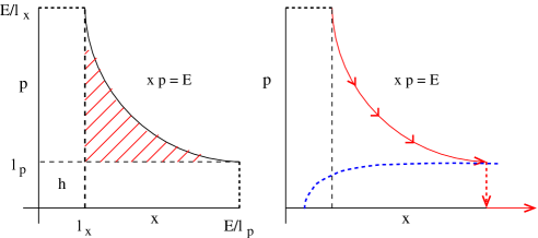
Figure 9: Left: allowed phase space region in the BK semiclassical quantization. Right: the dotted line represents the classical version of the state $\psi_{a}$ (187).

To complete this picture, let us try to understand the physical meaning of the state $\psi_{b}$ for $b(x)=1$. Writing

$$\psi_{b}(x)={1\over\sqrt{x}}\;{\rm sign}(x-1),$$ (189)

one finds that its time evolution under $H_{0}$ is given by

$$\psi_{b}(x,t)=e^{-itH_{0}}\psi_{b}(x)={1\over\sqrt{x}}\;{\rm sign}(x-e^{t}),$$ (190)

which is a kink state associated to the classical trayectory

$$x(t)=x_{0}\,e^{t},\;\;p(t)=0,\;\;E=x(t)p(t)=0$$ (191)

$H_{0}$ does not have a zero energy eigenstate, but based on these results one can think of $\psi_{b}$ heuristically as that state. The $p=0$ line in phase space is the classical analogue of the state $\psi_{b}$, just like the lines $p=\pm l_{p}$ are the classical analogue of $\psi_{a}$. This interpretation allows us to understand heuristically, the BK-regularization. Indeed, take a particle with energy $E$, which at the initial time $t=0$ is at $x=1$ and $p=E$. Following the classical trayectories (2) this particle will reach at time $t_{1}$, the boundary $p(t_{1})=l_{p}$ and then suddenly loose all its momenta, $p(t_{1}+\epsilon)=0$ (see fig. 9). The phase space area involved in this evolution agrees basically with the calculation made by Berry and Keating. If this area is a integer multiple of $2\pi\hbar$, then there is a bound state. In the previous argument, one should strictely reverse the time arrow since the classical trayectories generated by $1/(xp)$ are the time-reversed of eqs. (2), but the result does not change. At the quantum level the existence of bound states is due to an interference effect. In the absence of this interference the boundary at $p=\pm l_{p}$ behaves as a “transparent” wall, and the particles do not return to their initial position. This situation corresponds to Connes picture where all the eigenstates are delocalized. In this manner, the Berry-Keating and Connes pictures may coexist in a coherent picture both semiclassically and quantally.

Finally, we would like to make a comment concerning the wave function (185), and its relation to the von Neumann and Wigner potentials, mentioned in section IV Galindo ; neumann-wigner ; simon ; arai ; cruz . A common feature of these potentials is their asymptotic behaviour, $\sin(r)/r$, where $r>>1$ is the radius. The potentials having a positive energy eigenstate form a submanifold. So that a fine-tuning of couplings is required. It is interesting to observe the similarity with the potential (185), and the sensitivity to the choice of couplings in order to have bound states.

VI.3 Potentials for the Riemann zeros

In reference BK1 Berry and Keating tried to replace the semiclassical regularization of $xp$ with quantum boundary conditions that would generate a discrete spectrum. A proposal is to use the dilation symmetry of $xp$, i.e.

$$x\rightarrow K\;x,\qquad p\rightarrow p/K,$$ (192)

where $K$ corresponds to an evolution after time $\log K$ as indicated by eq.(2) (see Aneva for a discussion of the symmetries of $H=xp$). The Hamiltonian $H_{0}$ (6), is the generator of the scale transformations:

$$\psi(K\,x)={1\over K^{{1\over 2}-iH_{0}}}\;\psi(x).$$ (193)

Based on this, BK considered a linear superposition of the wave function $\psi_{E}(x)=Cx^{-1/2+iE}$ with the ones obtained by integer dilations $K=m$,

$$\psi_{E}(x) \rightarrow \sum_{m=1}^{\infty}\psi_{E}(m\,x)$$

$$= {C\over x^{1/2-iE}}\;\sum_{m=1}^{\infty}{1\over m^{1/2-iE}}={C\over x^{1/2-iE}}\;\zeta({1\over 2}-iE),$$

so that the vanishing of (VI.3) could be interpreted as an eigencondition. However, there is no justification for that condition, nor it is clear its physical or geometrical meaning. The approach we have been following so far is to implement the boundary conditions in a dynamical manner, hence it is more natural to impose the symmetry under discrete dilations, not on the eigenfunctions but on the potentials. Consider the linear superposition of (185),

$$\psi_{a}(x) \rightarrow \sum_{m=1}^{\infty}\psi_{a}(m\,x)$$

$$= {c\over x}\sum_{m=1}^{\infty}{\sin(2\pi mx)\over\pi m}={c\over x}\left([x]-x+{1\over 2}\right),$$

where $[x]$ denotes the integer part of $x$. We have used the Fourier decomposition of the sawtooth function $[x]-x+1/2$. The Mellin transform of the potential $a(x)=\sqrt{x}\psi_{a}(x)$ associated to (VI.3) is given by

$$\widehat{a}(t) = \int_{1}^{\infty}dx\,x^{-1+it}\;a(x)$$

$$= {c\over{1\over 2}-it}\left(\zeta({1\over 2}-it)+{1\over{1\over 2}+it}-{1\over 2}\right),$$

where we have used Edwards

$$\zeta(s)=s\int_{1}^{\infty}dx\;{[x]-x+{1\over 2}\over x^{s+1}}+{1\over s-1}+{1\over 2},\;\;{\rm Re}\;s>0.$$ (197)

Choosing $b(x)=1$, the Jost function ${\cal F}_{1}(t)$, associated to (VI.3), in leading order in $t$, is given by

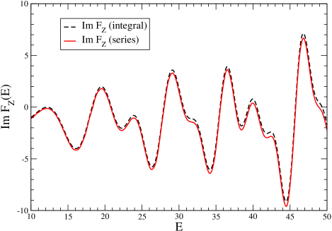
Figure 10: Numerical values of ${\rm Im}\;{\cal F}_{Z}(E)$ using two methods: 1) integrating (202) in the interval $(0,d)$ with $d=400$, and 2) Summing the series (203) up to $M=5000$.

$${\cal F}_{1}(t)\sim\left(1+{c\over 4}\right)^{2}-c\left(1+{c\over 4}\right)\;\zeta(1/2-it)-c^{2}\;S_{a_{0},a_{0}}(t),$$ (198)

where $S_{a_{0},a_{0}}$ denotes the function (137) with $\widehat{f}=\widehat{g}=a_{0}$, and

$$a_{0}(t)={\zeta(1/2-it)\over{1\over 2}-it}.$$ (199)

If $c=-4$, the Jost function ${\cal F}_{1}$ is given asymptotically by $S_{a_{0},a_{0}}$,

$${\cal F}_{1}(E)/4\sim{E^{2}\;Z(E)^{2}\over{1\over 4}+E^{2}}-iP\int_{-\infty}^{\infty}{dt\over\pi}\;{1\over t-E}\;{Et\;Z(t)^{2}\over{1\over 4}+t^{2}}.$$ (200)

A further approximation of (200) is

$${\cal F}_{1}(E)/4\sim{\cal F}_{Z}(E)=\,Z(E)^{2}-iP\int_{-\infty}^{\infty}{dt\over\pi}\;{\,Z(t)^{2}\over t-E},$$ (201)

or using that $Z(t)=Z(-t)$

$${\cal F}_{Z}(E)=\,Z(E)^{2}-2iE\;P\int_{0}^{\infty}{dt\over\pi}\;{\,Z(t)^{2}\over t^{2}-E^{2}},$$ (202)

The Cauchy integral, giving the imaginary part of ${\cal F}_{Z}(E)$, is convergent thanks to the asymptotic behaviour $|Z(t)|\sim|t|^{1/4+\epsilon}\;(\epsilon>0)$, on the critical line Titchmarsh2 . The integral (202) can be computed numerically in the interval $(0,d)$, with $d$ sufficiently large. The results converge rather slowly with $d$. Fig. 10 shows ${\rm Im}\;{\cal F}_{Z}(E)$ for $d=400$ in the interval $E\in(10,50)$.

An alternative method to find ${\rm Im}\;{\cal F}_{Z}(E)$ is to Hilbert transform $Z(t)^{2}$, using the well known series expansion of the zeta function,

$$\zeta(s)={1\over 2^{1-s}-1}\;\sum_{n=1}^{\infty}{(-1)^{n}\over n^{s}},\qquad{\rm Re}\;s>0.$$ (203)

After a long calculation one finds,

$${\rm Im}\,{\cal F}_{Z}(t)=-i\lim_{M\rightarrow\infty}$$ (204)

$$\left[{1\over p(t)\;p(-t)}\;\sum_{n,m}^{M}{(-1)^{n+m}\;{\rm sign}(n-m)\over n^{1/2-it}\;m^{1/2+it}}\right.$$

$$+{p(t)-p(-t)\over p(t)p(-t)}\sum_{n=1}^{M}{1\over n}$$

$$\left.-\sum_{n>m=1}^{M}{2\;(-1)^{n+m}\over n}\left({2^{(1/2+it)\{\log_{2}(n/m)\}}\over p(t)}-(t\rightarrow-t)\right)\right],$$

where $p(t)=2^{1/2+it}-1$ and $\{\log_{2}(n/m)\}$ is the fractional part of $\log_{2}(n/m)$. Fig.10 shows the values of ${\rm Im}\;{\cal F}_{Z}(E)$ computed with eq.(204), for $M=5000$ in the interval $E\in(10,50)$, which agrees reasonable well with the result obtained with the truncated integral (202). For larger values of $E$ it is more convenient to use the series expansion (204). The complete expression of ${\cal F}_{Z}(t)$ is obtained adding to (204), its real part $Z(t)^{2}$,

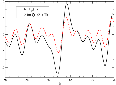
Figure 11: Numerical values of ${\rm Im}\;{\cal F}_{Z}(E)$ and ${\rm Im}\;\zeta(1/2-it)$ in the interval $E\in(50,75)$.

$${\cal F}_{Z}(t)=\lim_{M\rightarrow\infty}$$ (205)

$$\left[{2\over p(t)\;p(-t)}\;\sum_{n>m}^{M}{(-1)^{n+m}\over n^{1/2-it}\;m^{1/2+it}}\right.$$

$$+{1+p(t)-p(-t)\over p(t)p(-t)}\sum_{n=1}^{M}{1\over n}$$

$$\left.-\sum_{n>m=1}^{M}{2\;(-1)^{n+m}\over n}\left({2^{(1/2+it)\{\log_{2}(n/m)\}}\over p(t)}-(t\rightarrow-t)\right)\right],$$

As expected, eq. (205) does not have poles in the upper half plane. The poles arising from the terms proportional to $1/p(t)$ cancell each other.

The real part of ${\cal F}_{Z}(E)$ vanishes at the zeros of $Z(E)$. The question is wether its imaginary part, given by (204), also does. The answer to this question is negative in general, as can be seen from fig. 11, which plots the values of ${\rm Im}\;{\cal F}_{Z}(E)$, and those of $2\;{\rm Im}\zeta(1/2-iE)$ in the interval $(50,75)$. Observe that the shape of the two curves is similar, but their zeros do not coincide. Curiously enough, their maxima and minima are much closer. Fig. 12 displays the Argand plot of ${\cal F}_{Z}(E)$ and $\zeta(1/2-iE)$ in the interval $E\in(50,75)$. Observe again the similarity between their loop structures. We know of no reason why ${\rm Im}\;{\cal F}_{Z}(E)$ should vanish, even asymptotically, at the zeros of ${\rm Im}\;\zeta(1/2-iE)$ or $Z(t)$. If that were the case, then the Riemann zeros would become resonances with a life-time increasing asymptotically, but this seems unlikely. Our conclusion is that $\psi_{a}(x)$ (VI.3) is not enough to yield the Riemann zeros in the spectra, and that one needs a non trivial potential $b(x)$. A concrete proposal is to look for a ${\cal M}_{2}$ model yielding a Jost function ${\cal F}(t)$ proportional to $\zeta_{H}(1/2-it)$ ( recall (165)). We do not see at the moment any obstruction for this realization, but one needs additional insights.

Figure 12: Argand plane representation of ${\cal F}_{Z}(E)$ (left) and $\zeta(1/2-iE)$ (right) in the region $E\in(50,75)$. The loops associated to ${\cal F}_{Z}(E)$ do not generally passed through the origin and the are slightly displaced downward.

We shall end this section with some comments and suggestions.

• The function ${\cal F}_{Z}(t)$ (205), reminds a two-variable version of the zeta function first proposed by Euler

  $$\zeta(s_{1},s_{2})=\sum_{n_{1}>n_{2}>0}^{\infty}{1\over n^{s_{1}}_{1}\;n^{s_{2}}_{2}},$$ (206)

  if one chooses $s_{1}=1/2-it$ and $s_{2}=1/2+it$. Eq.(206), together with its multivariable extension, called Euler-Zagier zeta functions, have attracted much attention in various fields, as knot theory, perturbative quantum field theory, etc (see euler-zagier-1 , euler-zagier-2 and references therein). The function $\zeta(s_{1},s_{2})$ satisfies the so called shuffle relation

  $$\zeta(s_{1},s_{2})+\zeta(s_{2},s_{1})=\zeta(s_{1})\zeta(s_{2})-\zeta(s_{1}+s_{2}),$$ (207)

  which amounts in our case to the condition ${\cal F}_{Z}(t)+{\cal F}_{Z}(-t)=2Z(t)^{2}$. The two variable Euler-Zagier function can be meromorphically continued to $\vbox{\hbox{\upright\hbox to0.0pt{\hbox to0.0pt{C\hss}\kern 3.8pt\vrule height=8.0pt,width=0.4pt,depth=-0.1pt\hss}\phantom{C}}}^{2}$, except at the singularities $s_{1}=1$ and $s_{1}+s_{2}=2,1,0,-2,-4,\dots$. Hence, the identification $s_{1,2}=1/2\mp it$ is singular and a proper definition of $\zeta(s_{1},s_{2})$ requires a renormalization, probably along the lines of reference euler-zagier-2 using Hopf algebras.

• The results obtained in this section can be generalized to Dirichlet $L$-functions with real characters $\chi$ Davenport . We summarize briefly the main results. From the functional relation satisfied by the $L$-functions, it follows that the potentials, reproducing asymptotically the smooth positions of the zeros of $L(s,\chi)$, are given by

  $$a(x)\propto\left\{\begin{array}[]{ccc}\sin(\lambda x)/\sqrt{x},&&\chi:\;{\rm even}\\ \cos(\lambda x)/\sqrt{x},&&\chi:\;{\rm odd}\\ \end{array}\right.,$$ (208)

  which corresponds to the Bessel functions $J_{\nu}(\lambda x)$ with $\nu=\pm 1/2$. The value $\lambda$ is related to the period of the character $f$ as

  $$\lambda={2\pi\over f},\qquad\chi(n+f)=\chi(n),\;\;\forall n\in\vbox{\hbox{\upright\hbox to0.0pt{I\hss}\kern 1.7ptN}}.$$ (209)

  The generalization of (VI.3) is

  $$\psi_{a}(x)\rightarrow\sum_{m=1}^{\infty}\chi(m)\psi_{a}(m\,x)={c\over x}\sum_{m=1}^{\infty}{\chi(m)\over m}\left\{\begin{array}[]{c}\sin(\lambda mx)\\ \cos(\lambda mx)\\ \end{array}\right.,$$ (210)

  so that the characters $\chi(m)$ must be real. The corresponding Mellin transform of $a(x)=x^{1/2}\psi_{a}(x)$ is proportional to the Dirichlet function $L(1/2-it,\chi)$. As in the case of the zeta function, one also needs non trivial $b$ potentials to relate the Dirichlet functions to the Jost functions of the ${\cal M}_{2}$ model.

VII Conclusions

In this paper we have proposed a possible realization of the Hilbert-Pólya conjecture in terms of a Hamiltonian given by a perturbation of $H=xp$, or rather its inverse $1/(xp)$, by means of an antisymmetric matrix parameterize by two potentials $a(x)$ and $b(x)$. The Schrödinger equation can be reduced to a first order differential equation, suplemented with boundary conditions, which are exactly solvable in terms of a Jost function. In this respect, our approach is essentially different from the second order approaches to the RH based on standard QM.

The generic spectrum consists in a continuum of eigenenergies which may contain a point like spectra embbeded in it. We have studied a variety of examples showing that the existence of a point like spectrum depends “critically” on the values of the coupling constants of the model. We have found the potentials whose resonances approach the smooth Riemann zeros asymptotically. In the classical limit these potentials reproduce the Berry-Keating semiclassical regularization of $H=xp$. Implementing a discrete dilation symmetry on the previous potentials, we have obtained a Jost function which, in the asymptotic limit, resembles the two-variable Euler-Zagier zeta function $\zeta(s_{1},s_{2})$ with $s_{1,2}=1/2\mp it$. The real part of this Jost function vanishes at the Riemann zeros but not necessarily its imaginary part. These results were derived from a trivial potential $b(x)=1$, and they suggest that a non trivial choice of $b(x)$, could yield a Jost function directly related to the zeta function. A natural candidate is ${s-1\over s}\zeta(s)$, with $s=1/2-it$, which has the correct analiticity properties. If these potentials do exist, then the Riemann zeros would become bound states of the model and the RH would follow automatically. This is how the Hilbert-Pólya conjecture would come true in our approach.

References

- (1) H.M. Edwards, “Riemann’s Zeta Function”, Academic Press, New York, 1974.
- (2) E.C. Titchmarsh, “The Theory of the Riemann Zeta-Function”, 2nd ed., Oxford University Press 1999, Oxford.
- (3) E. Bombieri, “Problems of the Millenium: the Riemann hypothesis”, Clay Mathematics Institute (2000).
- (4) P. Sarnak, “Problems of the Millenium: the Riemann hypothesis (2004)”, Clay Mathematics Institute (2004).
- (5) J.B. Conrey, ”The Riemann Hypothesis.” Not. Amer. Math. Soc. 50, 341-353, 2003.
- (6) See M. Watkins at http://secamlocal.ex.ac.uk/mwatkins /zeta/physics.htm for a comprehensive review on several approaches to the RH.
- (7) H.C. Rosu, “Quantum hamiltonians and prime numbers”, Mod. Phys. Lett. A18 (2003) 1205; quant-ph/0304139.
- (8) E. Elizalde, V. Moretti, S. Zerbini, “On recent strategies proposed for proving the Riemann hypothesis”, Int.J.Mod.Phys. A18 (2003) 2189-2196; math-ph/0109006.
- (9) A. Selberg, ”Harmonic analysis and discontinuous groups in weakly symmetric Riemannian spaces with applications to Dirichlet series”, Journal of the Indian Mathematical Society 20 (1956) 47-87.
- (10) H. Montgomery, “The pair correlation of zeros of the zeta function”, Analytic Number Theory, AMS (1973).
- (11) A. Odlyzko, “On the distribution of spacings between zeros of zeta functions”, Math. Comp. 48, 273 (1987).
- (12) M.V. Berry, in Quantum Chaos and Statistical Nuclear Physics. Eds. T.H. Seligman and H. Nishioka, Lecture Notes in Physics, No. 263, Springer Verlag, New York, 1986.
- (13) M. C. Gutzwiller ”Periodic orbits and classical quantization conditions”, J. Math. Phys. 12 no. 3 (1971).
- (14) B. Julia, “Statistical theory of numbers”, in Number Theory and Physics, Springer Proceedings in Physics, 47 (1990).
- (15) J.-B. Bost and A. Connes, “Hecke algebras, Type III factors and phase transitions with spontaneous symmetry breaking in number theory”. Selecta Mathematica, New Series 1, No. 3, 411, (1995).
- (16) G. Mussardo, “The Quantum Mechanical Potential for the Prime Numbers”, cond-mat/9712010.
- (17) M.V. Berry and J.P. Keating, “H=xp and the Riemann zeros”, in Supersymmetry and Trace Formulae: Chaos and Disorder, ed. J.P. Keating, D.E. Khmelnitskii and I. V. Lerner, Kluwer 1999.
- (18) M. V. Berry and J. P. Keating, “The Riemann zeros and eigenvalue asymptotics”, SIAM REVIEW 41 (2) 236, 1999.
- (19) A. Connes, “Trace formula in noncommutative geometry and the zeros of the Riemann zeta function”, Selecta Mathematica (New Series) 5 (1999) 29; math.NT/9811068.
- (20) G. Sierra, “The Riemann zeros and the Cyclic Renormalization Group”, J.Stat.Mech. 0512 (2005) P006; math.NT/0510572.
- (21) A. LeClair, J.M. Román and G. Sierra, “Russian doll Renormalization Group and Superconductivity”, Phys. Rev. B69 (2004) 20505; cond-mat/0211338.
- (22) A. Anfossi, A. LeClair, G. Sierra, “The elementary excitations of the exactly solvable Russian doll BCS model of superconductivity”, J. Stat. Mech. (2005) P05011; cond-mat/0503014.
- (23) C. Dunning and J. Links, “Integrability of the Russian doll BCS model”, Nucl. Phys. B702 (2004) 481, cond-mat/0406234.
- (24) S. D. Glazek and K. G. Wilson, “Limit cycles in quantum theories”, Phys. Rev. Lett. 89 (2002) 230401, hep-th/0203088; “Universality, marginal operators, and limit cycles”, Phys. Rev. B69, 094304 (2004); cond-mat/0303297.
- (25) D. Bernard and A. LeClair, “Strong-weak coupling duality in anisotropic current interactions”, Phys.Lett. B512 (2001) 78; hep-th/0103096.
- (26) P. F. Bedaque, H.-W. Hammer, and U. van Kolck, “Renormalization of the Three-Body System with Short-Range Interactions”, Phys. Rev. Lett. 82 (1999) 463, nucl-th/9809025.
- (27) E. Braaten and H.-W. Hammer, “ Universality in Few-body Systems with Large Scattering Length”, Phys.Rept. 428 (2006) 259-390, cond-mat/0410417.
- (28) A. Morozov and A. J. Niemi, “Can Renormalization Group Flow End in a Big Mess?”, Nucl. Phys. B666, 311 (2003); hep-th/0304178.
- (29) A. LeClair, J.M. Román and G. Sierra, “Russian doll Renormalization Group and Kosterlitz-Thouless Flows”, Nucl. Phys. B675 (2003) 584; hep-th/0301042.
- (30) A. LeClair, J.M. Román and G. Sierra, “Log-periodic behaviour of finite size effects in field theory models with cyclic renormalization group”, Nucl. Phys. B700 [FS] (2004) 407; hep-th/0312141.
- (31) A. LeClair,and G. Sierra, “Renormalization group limit-cycles and field theories for elliptic S-matrices”, Theor. Exp. (2004) P08004; hep-th/0403178.
- (32) A. LeClair, “Interacting Bose and Fermi gases in low dimensions and the Riemann hypothesis”; math-ph/0611043.
- (33) A. Galindo and P. Pascual, “Quantum Mechanics I, II”, Springer Verlag, Berlin 1990-1991.
- (34) J. von Neumann, “Allgemeine Eigenwerttheorie Hermitescher Funktionaloperatoren”, Math. Ann. 102, 49-131, (1929).
- (35) J. Twamley and G. J. Milburn, “The quantum Mellin transform”, New J. Phys. 8 (2006) 328.
- (36) N.N. Khuri, “Inverse Scattering, the Coupling Constant Spectrum, and the Riemann Hypothesis”, Math. Phys. Anal. Geom. 5 (2002) 1-63; hep-th/0111067.
- (37) K. Chadan and M. Musette, ”On an interesting singular potential”, C.R. Acad. Sci. Paris 316 II, 1 (1993).
- (38) J. von Neumann and E. P. Wigner, “Über Merkwürdige Diskrete Eigenwerte”, Z. Phys. 30 (1929) 465-467.
- (39) B. Simon, “On positive eigenvalues of one body Schrödinger operators”, Comm. Pure. Appl. Math. 12 (1969) 531-538.
- (40) M. Arai and J. Uchiyama, “On the von Neumann and Wigner Potentials”, J. Diff Eq. 157 (1999) 348-372.
- (41) J. Cruz-Sampedro, I. Herbst, R. Martínez-Avendaño, “Perturbations of the Wigner-Von Neumann potential leaving the embedded eigenvalue fixed”, Annales Henri Poincar 3 (2002), 331-345.
- (42) L. S. Gradshteyn and I.M. Ryzhik, “Table of integrals, series and products”, 6th ed. Academic Press, 2000, London.
- (43) E.C. Titchmarsh, “Introduction to the theory of Fourier integrals”, Oxford University Press (1937), 2nd ed. New York.
- (44) G.B. Arfken and H.J. Weber, “Mathematical Methods for Physicist”, Elsevier Academic Press (2005),6th ed. Oxford.
- (45) “Encyclopedic Dictionary of Mathematics”, vol I, MIT Press (1977). The Mathematical Society of Japan.
- (46) , P.L. Duren, “Theory of Spaces”. Academic Press, New York, 1970.
- (47) J. F. Burnol, “An adelic causality problem related to abelian L-functions”, J. Number Theory 87 (2001), no. 2, 253-269; math.NT/0001013.
- (48) J. F. Burnol, “On Fourier and Zeta(s)” Forum Mathematicum 16 (2004), 789-840; math.NT/0112254.
- (49) B.S. Pavlov and L.D. Faddeev, “Scattering theory and automorphic functions”, Sov. Math. 3, 522 (1975), Plenum Publishing Corp. translation, N.Y;
- (50) Lax and R.S. Phillips, Scattering Theory for Automorphic Functions, Princeton University Press, Princeton, 1976.
- (51) M.C. Gutzwiller, “Stochastic behaviour in Quantum Scattering”, Physica D7, 341 (1983).
- (52) S. Joffily, “Jost function, prime numbers and Riemann zeta function”, math-ph/0303014
- (53) R.K. Bhaduri, Avinash Khare, and J. Law, ”Phase of the Riemann zeta function and the inverted harmonic oscillator”, Physical Review E 52 no. 1 (1995) 486-491; chao-dyn/9406006.
- (54) B. Aneva, “Symmetry of the Riemann operator”, Phys. Lett. B 450 (1999) 388.
- (55) S. Akiyama and Y. Tanigawa, “Multiple zeta values at non-positive integers”, Ramanujan J. 5 (2001), 327-351.
- (56) L. Guo and B. Zhang, “Renormalization of Multiple zeta values”, math.NT/0606076.
- (57) H. Davenport, “Multiplicative Number Theory”, 2nd ed., Springer-Verlag, New York, 1980.