Discrete and continuous exponential transforms
of simple Lie groups of rank two

Abstract.

We develop and describe continuous and discrete transforms of class functions on compact simple Lie group $G$ as their expansions into series of uncommon special functions, called here $\,\mathop{\operatorname{{E}}}\nolimits$-functions in recognition of the fact that the functions generalize common exponential functions. The rank of $\,G\,$ is the number of variables in the $\,\mathop{\operatorname{{E}}}\nolimits$-functions. A uniform discretization of the decomposition problem is described on lattices of any density and symmetry admissible for the Lie group $G$.

1. Introduction

The aim of this paper is to generalize common exponential functions in one variable $x$,

$$\mathop{\operatorname{{E}}}\nolimits_{m}(x):=e^{imx}\,,\quad m\in\mathbb{Z}\,,\ x\in\mathbb{R}\,,$$ (1.1)

together with the corresponding Fourier transform,

$$f(x)=\sum_{m=0}^{\infty}b_{m}e^{imx}\,,\qquad b_{m}=\frac{1}{2\pi}\int_{0}^{2\pi}f(x)e^{-imx}\,dx\,,$$ (1.2)

to any number of variables.

For close to two centuries functions (1.1) have been part of Fourier analysis. Crucial property is their pairwise orthogonality when integrated over a range $a\leq x\leq a+2\pi$ with any $a\in\mathbb{R}$. More recent but equivalent interpretation of the functions is as irreducible characters of the 1-parametric unitary group $\mathop{\operatorname{{U}}}\nolimits(1)$. There is yet another interpretation of the functions (1.1), rather trivial in this case, which nevertheless is the departure point for our generalization. It is presented in the example of Section 3.

The simplest possible $n$-dimensional generalization of exponential functions, is based on the $n$-fold product $\mathop{\operatorname{{U}}}\nolimits(1)\times\mathop{\operatorname{{U}}}\nolimits(1)\times\cdots\times\mathop{\operatorname{{U}}}\nolimits(1)$. Corresponding functions are products of $n$ copies of $\mathop{\operatorname{{E}}}\nolimits_{m}(x)$, each depending on its own continuous variable $x$ and its own lattice variable $m$. It is undoubtedly useful and it is frequently used. However we are not concerned with such a generalization in this paper.

Underlying symmetry group of $\mathop{\operatorname{{E}}}\nolimits$-functions in this article is any compact semisimple Lie group $G$ of rank $n$ in general. The rank of $G$ is the number of continuous variables. Here our considerations are focused on the three simple Lie groups of rank 2, namely $\mathop{\operatorname{{SU}}}\nolimits(3)$, $\mathop{\operatorname{{O}}}\nolimits(5)$ (or $\mathop{\operatorname{{Sp}}}\nolimits(4))$, and $\mathop{\operatorname{{G}}}\nolimits(2)$. Our aim is to describe the three cases in a ready-to-use form.

There are two papers dealing briefly with $\mathop{\operatorname{{E}}}\nolimits$-functions: Their definition appeared in [1], and their orthogonality is proven in [2]. We know of no other attempt in the literature to generalize exponential functions to more than one variable.

First however let us underline a close relation of the $\mathop{\operatorname{{E}}}\nolimits$-functions of this paper with the $\mathop{\operatorname{{C}}}\nolimits$- and $\mathop{\operatorname{{S}}}\nolimits$-functions of [3, 4, 5, 6, 7]. All three families of functions are based on a semisimple compact Lie group $G$. They are constructed by summation of appropriate products of $\mathop{\operatorname{{U}}}\nolimits(1)$ characters over an orbit of a relevant finite group. It is the Weyl group $W$ of $G$ in case of $\mathop{\operatorname{{C}}}\nolimits$- and $\mathop{\operatorname{{S}}}\nolimits$-functions, and it is the even subgroup $W_{e}\subset W$ of $G$ in case of the $\mathop{\operatorname{{E}}}\nolimits$-functions. Furthermore, due to the relation of the three families to the group elements of the maximal torus of the underlying Lie group, one gets the symmetries of the functions with respect to both affine Weyl group $W^{\mathop{\operatorname{{aff}}}\nolimits}$ and even affine Weyl group $\,W_{e}^{\mathop{\operatorname{{aff}}}\nolimits}.$

For comparison with (1.1), let us point out that 1-dimensional $\mathop{\operatorname{{C}}}\nolimits$- and $\mathop{\operatorname{{S}}}\nolimits$-functions are (up to a normalization) the familiar trigonometric functions

$$\mathop{\operatorname{{C}}}\nolimits_{m}(x)\sim\cos mx,\quad\mathop{\operatorname{{S}}}\nolimits_{m}(x)\sim\sin mx\,,\quad m\in\mathbb{Z}^{\geq 0}\,,\ x\in\mathbb{R}\,.$$

Within either $\mathop{\operatorname{{C}}}\nolimits$- or $\mathop{\operatorname{{S}}}\nolimits$-family, the functions are pairwise orthogonal in $a\leq x\leq a+\pi$. The underlying Lie group is $\mathop{\operatorname{{SU}}}\nolimits(2)$ for both families.

Recently $\mathop{\operatorname{{C}}}\nolimits$-functions were studied relatively extensively. Their properties are reviewed in [6] (see also references therein), similarly the $\mathop{\operatorname{{S}}}\nolimits$-functions are found in [1, 2, 7]. Let us as well point out that some properties of functions symmetrized over a finite group in general are described by I. Macdonald, [8].

It may appear (falsely) that the expansions, based on compact semisimple Lie groups, impose severely constraining requirements on functions amenable to such expansions. Typically one is interested in expansions of a function given on a finite region, say $R$, of a real Euclidean space $\mathbb{R}^{n}$ either as a continuous function (‘continuous data’) or by its values at lattice points in $R$ (‘digital data’). In our approach one first needs to choose a semisimple Lie group of rank $n$ whose weight lattice has the same geometric structure as the lattice of the data (there is always at least one such group). Then the region $R$ is inserted into the fundamental region $F$ of the chosen Lie group $R\subset F$. In the case of digital data, a unique aspect of our method is the easy possibility to match the density of the data points in $R$ by the density of a grid $F_{M}$ in $F$. More precisely, the positive integer $M$ selects a finite Abelian subgroup of the Lie group such that its conjugacy classes are represented by the points of $F_{M}$.

The families of $\mathop{\operatorname{{C}}}\nolimits$-, $\mathop{\operatorname{{S}}}\nolimits$-, and $\mathop{\operatorname{{E}}}\nolimits$-functions have a number of properties in common. In addition to their orthogonality, when integrated over a finite region $F$ of an Euclidean space $\mathbb{R}^{n}$, they are also discretely orthogonal when summed up over a discrete grid $F_{M}\subset F$. Discrete orthogonality of $\mathop{\operatorname{{C}}}\nolimits$-functions in general is the main content of [9]. Furthermore, the lattice, obtained when $F_{M}$ is extended to the whole space $\mathbb{R}^{n}$, is setup uniformly for all three families. Density of such a lattice is specified by a positive integer $M$. Functions of the three families are eigenfunctions of the same Laplace operator, namely the one appropriate for the group $G$, differing mainly by their behavior at the boundary of $F$. Their eigenvalues are known explicitly for all $n$ and all three families. Their products are decomposable into their sums. The functions can be built up recursively (in lattice variables), for any number of variables $x\in\mathbb{R}^{n}$, by a judicious choice of the lowest few and by their successive multiplication. In principle they could be also built recursively in the points of $F_{M}$ (for the same lattice variable), using the fact that the points of $F_{M}$ stand for conjugacy classes of a finite Abelian group, although it could be a laborious way to do it.

Discrete orthogonality of $\mathop{\operatorname{{C}}}\nolimits$-functions, see [9], were exploited in challenging mathematical applications, see [10] and references therein. Immediate motivation of our current interest in the three families of functions arose as a result of the observation made in [11, 12, 13] that continuous extensions of the (finite) discrete expansions of functions on $F_{M}$ smoothly interpolate digital data between discrete points. Such an observation is strongly supported by numerous convincing examples and qualitative arguments in case of $\mathop{\operatorname{{C}}}\nolimits$-functions and certainly carries over to $\mathop{\operatorname{{S}}}\nolimits$-functions. However, a quantitative demonstration has yet to be made even in those cases.

In two dimensions practical need to interpolate digital data lead to development of a number of sophisticated interpolation methods. Comparison of such methods with ours depends on the model functions one compares it with. In general, one may say that the precision of the best interpolation methods is comparable to ours. However, unlike our approach, none of these methods readily generalizes to higher dimensions. In our case all one needs is to replace one compact semisimple Lie group of rank two by another one of rank $\,n<\infty$.

Generalization of the $\mathop{\operatorname{{E}}}\nolimits$-transform from one to more dimensions in case of a semisimple Lie group which is not simple, say $G=G_{1}\times G_{2}$, presents two interesting options, each worth to be explored. The fundamental region $F^{e}$, where the expansion takes place, and the expansion functions are different. In spite of that one has in both cases the continuous and discrete orthogonality of the functions in $F^{e}$. The simpler option of the two is followed up in this paper.

In Section 2 we recall briefly the definition of the Weyl group of simple (or semisimple) Lie group and its affine Weyl group and their basic properties. Also we define the subgroup of even elements of the Weyl group $\,W_{e}\,$ and the corresponding even affine Weyl group together with their root lattice, fundamental region, etc. In Section 3 we introduce $\,\mathop{\operatorname{{E}}}\nolimits$-functions $\mathop{\operatorname{{E}}}\nolimits_{\lambda}(x)$ of a Weyl group. The functions are specified by a given point $\lambda\in\mathbb{R}^{n}$. Their $\,W_{e}\,$-invariance is shown. Also, analogously to the case of both $\,\mathop{\operatorname{{C}}}\nolimits$- and $\,\mathop{\operatorname{{S}}}\nolimits$-functions, $\,\mathop{\operatorname{{E}}}\nolimits$-functions are orthogonal over the fundamental region $\,F^{e}\subset\mathbb{R}^{n}$ of $\,W_{e}$. The general method of expansion of a function on $\,F\,$ into the sum of orthogonal $\,\mathop{\operatorname{{E}}}\nolimits$-functions is given. We illustrate it on the case of the rank one Lie group $\,\mathop{\operatorname{{A_{1}}}}\nolimits$. In Section 4 the $\,\mathop{\operatorname{{E}}}\nolimits$-functions together with their continuous transforms are described for the three simple Lie groups of rank $\,2$. Discrete orthogonality of $\,\mathop{\operatorname{{E}}}\nolimits$-functions in general is the content of Section 5, while in Section 6 pertinent properties are described for exploitation of continuous extensions of discrete $\mathop{\operatorname{{E}}}\nolimits$-expansions of functions on the fundamental region $\,F^{e}\,$ for the simple Lie groups of rank two. The decomposition of the product of $\,\mathop{\operatorname{{E}}}\nolimits$-functions for these groups is the subject of Section 7. Finally, in Section 8 we introduce central splitting of functions given on $F$ or $F_{M}$ into the sum of $\,s\,$ functions, where $\,s\,$ is the order of the center of the corresponding Lie group. Each component function has simpler $\,\mathop{\operatorname{{E}}}\nolimits$-functions expansions. Concluding remarks and some related problems are brought forward in Section 9.

2. Weyl group, its even subgroup and their affininizations

Let $\,r_{i}\,$ be reflection transformation of $\,\mathbb{R}^{n}\,$ with respect to $\,n-1$-dimensional subspace containing the origin. Consider finite groups $\,W\,$ generated by $\,n\,$ such reflections $\,r_{1},r_{2},\dots,r_{n}$. For any point $\,\lambda\in\mathbb{R}^{n}\,$ we define the orbit $\,W(\lambda)\,$ of the point $\,\lambda\,$ under the action of $\,W\,$ as the set of all different points of the form $\,\omega\lambda,$ $\,\omega\in W$. Then the corresponding orbit function is the following

$$\mathop{\operatorname{{C}}}\nolimits_{\lambda}(x)=\sum_{\mu\in\,W(\lambda)}e^{2\pi i\langle\,\mu,x\rangle}\,,\qquad x\in\mathbb{R}^{n},$$ (2.1)

where $\,\langle\ ,\ \rangle\,$ is a scalar product in $\,\mathbb{R}^{n}$. Note that for $\,n=1\,$ we have $\,\mathop{\operatorname{{C}}}\nolimits_{\lambda}(x)=2\cos(\pi mx)$, where $\,m\in\mathbb{Z}^{\geq 0}\,$ and $\,x\in\mathbb{R}$.

In this paper we consider $\,\mathop{\operatorname{{E}}}\nolimits$-functions which are orbit functions corresponding to symmetry group $\,W_{e}\,$ of even elements of Weyl groups of simple (or semisimple) Lie group. Below we recall some basic definition about both Lie groups and corresponding Weyl groups. For further information about both simple Lie groups and the Weyl groups we refer to the books [15], [16].

The Weyl group $\,W\,$ of any simple (or semisimple) Lie group is specified by its Coxeter-Dynkin diagrams. The diagram is a concise way to give a certain non-orthogonal basis $\,\Pi=\{\alpha_{1},\dots,\alpha_{n}\}\,$ in $\,\mathbb{R}^{n}$. Each node of the diagram is associated with a basis vector $\,\alpha_{k}\,$, called the simple root of the Lie group. Acting by elements of the Weyl group $\,W\,$ upon simple roots, we obtain a finite system of vectors, which is invariant with respect to $\,W$. A set of all such vectors is called the root system $\,\Delta\,$ associated with a given Coxeter-Dynkin diagram. The set of all linear combinations

$$Q=\left\{\sum_{i=1}^{n}a_{i}\alpha_{i}\ |\,a_{i}\in\mathbb{Z}\right\}=\bigoplus_{i=1}^{n}\mathbb{Z}\alpha_{i}$$ (2.2)

is called the root lattice. Relative lengths and angles between simple roots of the basis $\,\Pi\,$ are specified in terms of the elements of the Cartan matrix $\,C=(c_{ij})_{i,j=1}^{n}\,,$ where

$$c_{ij}=\tfrac{2\langle\alpha_{i}|\alpha_{j}\rangle}{\langle\alpha_{j}|\alpha_{j}\rangle}=\langle\alpha_{i}|\check{\alpha}_{j}\rangle,\quad{\rm for}\quad i,j=1,\dots,n.$$

Here $\,\check{\alpha}_{j}\,$ is the simple root of the dual root system $\,\check{\Delta}=\{\check{\alpha}=2\alpha/\langle\alpha,\alpha\rangle\ |\ \alpha\in\Delta\}$. Denote by $\,\check{Q}\,$ the corresponding coroot lattice. Absolute length for the roots is chosen by an additional convention, namely that the longer roots of $\,\Pi\,$ satisfy $\,\langle\alpha|\alpha\rangle=2$. In addition to the $\,\alpha$-basis it is convenient to introduce the basis of fundamental weights $\,\omega_{1},\dots,\omega_{n}$. The $\,\omega$-basis and $\,\alpha$-basis are related by the inverse of the Cartan matrix

$$\omega_{j}=\sum_{k=1}^{n}(C^{-1})_{jk}\alpha_{k}.$$

Analogously to the root lattice we introduce the weight lattice

$$P=\left\{\sum_{i=1}^{n}a_{i}\omega_{i}\ |\,a_{i}\in\mathbb{Z}\right\}=\bigoplus_{i=1}^{n}\mathbb{Z}\omega_{i}\,.$$

We also define the set of dominant weights $\,P^{+}\,$ and the set of strictly dominant weights $\,P^{++}\,$

$$P^{+}=\mathbb{Z}^{\geq 0}\omega_{1}+\mathbb{Z}^{\geq 0}\omega_{2}+\dots+\mathbb{Z}^{\geq 0}\omega_{n}\ \supset\ P^{++}=\mathbb{Z}^{>0}\omega_{1}+\mathbb{Z}^{>0}\omega_{1}+\dots+\mathbb{Z}^{>0}\omega_{1}.$$ (2.3)

For each $\,\alpha\in\Delta\,$ and integer $\,k\,$ we define the hyperplane

$$H_{\alpha,\,k}=\{t\in\mathbb{R}_{n}\,|\,\langle t,\alpha\rangle=k\}$$

and the associated reflection $\,r_{\alpha,\,k},$ in the hyperplane $\,H_{\alpha,\,k}\,$

$$r_{\alpha,\,k}\,x=x-\langle\alpha,\,x\rangle\check{\alpha}+k\check{\alpha}.$$ (2.4)

The finite Weyl group $\,W\,$ is generated by $\,r_{\alpha,\,0},$ $\,\alpha\in\Pi$. Since the action of $\,W\,$ on $\,\Pi\,$ gives the root system $\,W\Pi=\Delta$, $\,W\,$ can be extended to the affine Weyl group $\,W^{\mathop{\operatorname{{aff}}}\nolimits}\,$, the group generated by $\,r_{\alpha,\,k}\,$ for all $\,\alpha\in\Pi\,$ and $\,k\in\mathbb{Z}$. $\,W^{\mathop{\operatorname{{aff}}}\nolimits}\,$ is an infinite group such that

$$\,W^{\mathop{\operatorname{{aff}}}\nolimits}=\check{Q}\rtimes W$$ (2.5)

It is the semidirect product of its subgroups $\,W\,$ and the invariant Abelian subgroup $\,\check{Q}\,$, the coroot lattice, for proof see [16].

For any Weyl group there exists a unique highest root

$$\xi_{h}=\sum_{i=1}^{n}m_{i}\alpha_{i}\equiv\sum_{i=1}^{n}q_{i}\check{\alpha}_{i}.$$

Coefficients $\,m_{i}\,$ and $\,q_{i}\,$ are called marks and comarks correspondingly and could be found in [17]

Finally, for any affine Weyl group we introduce its fundamental domain (or region) $\,F\subset\mathbb{R}^{n}\,$ as the convex hull of $\,\{0,\,\tfrac{\check{\omega}_{1}}{q_{1}},\dots,\tfrac{\check{\omega}_{n}}{q_{n}},\}$ where $\,q_{1},\dots,q_{n}$. By definition $\,F\,$ is closed. If $\,G\,$ is not simple then its fundamental region is the Cartesian product of fundamental regions of its simple components.

2.1. Subgroup of even elements of the Weyl group $\,W_{e}\,$ and its affine group $W_{e}^{\mathop{\operatorname{{aff}}}\nolimits}$

Let $\,W\,$ be a Weyl group of simple Lie group. This group is generated by reflection transformations $\,r_{i},\,$ $i=1,\dots,n$. We consider the subset of $\,W\,$

$$W_{e}=\langle r_{i_{1}}\dots r_{i_{p}}|\ p\ {\rm is\ even},\ i_{j}\in\{1,\dots,n\}\rangle,$$

i.e. the set of elements generated by even number of reflections, or the elements of $\,W\,$ of even length. Obviously, $\,W_{e}\,$ forms a finite normal subgroup of $\,W$ of index $\,2\,$, such that

$$W=W_{e}\dot{\cup}\bigcup_{i=1}^{n}r_{i}W_{e}\equiv W_{e}\dot{\cup}r_{i}W_{e},\qquad|W_{e}|=\tfrac{1}{2}|W|.$$ (2.6)

The index $\,i\,$ in the last equation is arbitrary, since $\,r_{j}{r_{i}}^{-1}\in W_{e}\,$ for any $i,j\in\{1,\dots,n\}$. For an arbitrary point $\,\lambda\,$ in $\,\mathbb{R}^{n}$ we denote by $\,W_{e}(\lambda)\,$ its orbit with respect to the action of the even Weyl group. Every $\,\lambda\,$ is contained in precisely one $\,W_{e}$-orbit. From [6] it follows that each original $\,W$-orbits contains a unique $\,\mu\in P^{+}$. By (2.6) we obtain that each $\,W_{e}$-orbit contains a unique element belonging to $\,P_{e}:=P^{+}\cup r_{i}P^{++}$. The $\,W$- and $\,W_{e}$-orbits are in the following correspondence with the orbits of original Weyl groups:

$$W(\lambda)=\begin{cases}W_{e}(\lambda)\cup W_{e}(r_{i}\lambda),&\text{if $\,\lambda\in P^{++}$}\quad{\rm for\ some\ }\ i\in\{1,\dots,n\}\\ W_{e}(\lambda),&\text{if $\,\lambda\in P^{+}\setminus P^{++}.$}\end{cases}$$ (2.7)

In particular, let we denote by $\,|W_{e}(\lambda)|\,$ the size of the orbit $\,W_{e}(\lambda)\,$, then $\,|W_{e}(\lambda)|\,$ is either equal to $\,|W(\lambda)|\,$ or to $\,\tfrac{1}{2}|W(\lambda)|\,$.

Consider the original affine group $\,W^{\mathop{\operatorname{{aff}}}\nolimits}\,$ generated by $\,r_{\alpha,\,k}\,$ defined in (2.4). Then the even affine group is the subgroup of words of even length in $\,r_{\alpha,\,k}\,$ of $\,W^{\mathop{\operatorname{{aff}}}\nolimits}\,$, i.e.

$$W_{e}^{\mathop{\operatorname{{aff}}}\nolimits}=\langle r_{\alpha_{i_{1}},\,k_{1}}\dots r_{\alpha_{i_{p}},\,k_{p}}|\ p\ {\rm is\ even},\ \alpha_{i_{j}}\in\Pi,\ k_{i}\in\mathbb{Z}\rangle.$$ (2.8)

As in the case of original affine Weyl group we have the following relation between $\,W_{e}^{\mathop{\operatorname{{aff}}}\nolimits}\,$ and $\,W_{e}\,$

$$W_{e}^{\mathop{\operatorname{{aff}}}\nolimits}=\check{Q}\rtimes W_{e}.$$ (2.9)

Indeed, the subgroup of $\,W_{e}^{\mathop{\operatorname{{aff}}}\nolimits}\,$ generated by $\,r_{\alpha,\,0}\,$ coincides with $\,W_{e}$, therefore $\,W_{e}<W_{e}^{\mathop{\operatorname{{aff}}}\nolimits}$. For any element $\,d\in\mathbb{R}^{n}\,$ define a translation

$$\begin{array}[]{c}\tau(d)\,x=x+d,\qquad x\in\mathbb{R}^{n}\end{array}$$

For any two $\,d,d^{\prime}\in\mathbb{R}^{n}\,$ $\,\tau(d)\,\tau(d^{\prime})=\tau(d+d^{\prime})$, therefore we may identify $\,\check{Q}\,$ with a group of translations on $\,\mathbb{R}^{n}\,$. Since

$$r_{\alpha,\,k}=\tau(k\check{\alpha})r_{\alpha,\,0}$$ (2.10)

we obtain that for $\,\alpha\in\Pi\,$ and $\,k\in\mathbb{Z}\,$ $\,\tau(k\check{\alpha})=r_{\alpha,\,k}r_{\alpha}^{-1}\in W_{e}^{\mathop{\operatorname{{aff}}}\nolimits}$. In particular for any $\,i=1,\dots,n\,$ $\,\tau(\check{\alpha_{i}})\in W_{e}^{\mathop{\operatorname{{aff}}}\nolimits}\,$ and therefore $\,\check{Q}\in W_{e}^{\mathop{\operatorname{{aff}}}\nolimits}$. Further, from (2.10) follows that $\,W_{e}^{\mathop{\operatorname{{aff}}}\nolimits}=W_{e}\,\check{Q}\,$. Also since any non-zero element of $\,\check{Q}\,$ has infinite order and any non-zero element of $\,W_{e}\,$ has finite order we obtain that $\,W_{e}\cap\check{Q}={0}$. Finally, we have to show that subgroup $\,\check{Q}\,$ is normal in $\,W_{e}^{\mathop{\operatorname{{aff}}}\nolimits}$. Indeed, for any $\,w\in W_{e}\subset W\,$ and any $\,d\in\check{Q}\,$ we have $\,w\,\tau(d)w^{-1}=\tau(wd)\,$.

Using (2.6) we also can define now the fundamental domain of $\,W_{e}^{\mathop{\operatorname{{aff}}}\nolimits}\,$ being a set

$$F^{e}=F\cup r_{i}F.$$ (2.11)

3. Definition of $\,\mathop{\operatorname{{E}}}\nolimits$-functions, their relations to $\,\mathop{\operatorname{{C}}}\nolimits$-functions

We start with the definition (2.1) of $\,\mathop{\operatorname{{C}}}\nolimits$-functions. The $\,\mathop{\operatorname{{C}}}\nolimits$-function $\mathop{\operatorname{{C}}}\nolimits_{\lambda}(x)$ is the contribution to an irreducible character from the orbit $\,W(\lambda)\,$, $\lambda\in P^{+}$. If in (2.1) we restrict ourselves to the orbit $\,W_{e}(\lambda)\,$ instead of the orbit of $W$, we obtain the $\,\mathop{\operatorname{{E}}}\nolimits$-function $\mathop{\operatorname{{E}}}\nolimits_{\lambda}(x)$:

$$\mathop{\operatorname{{E}}}\nolimits_{\lambda}(x)=\sum_{\mu\in\,W_{e}(\lambda)}e^{2\pi i\langle\mu,\,x\rangle}\ ,\qquad{\rm for\ }x\in\mathbb{R}^{n},\quad\lambda\in P.$$ (3.1)

The $\,\mathop{\operatorname{{C}}}\nolimits$-functions appeared in [9, 6] under the name ”orbit functions”. Their many properties, very useful for applications, were extensively studied i n [1]-[6]. In this section we formulate analogous properties of $\,\mathop{\operatorname{{E}}}\nolimits$-functions.

To start, both families of $\,\mathop{\operatorname{{C}}}\nolimits$- and $\,\mathop{\operatorname{{E}}}\nolimits$-functions are based on semisimple Lie algebra, the rank of the algebra is the number of variables. They are given as the finite sums of exponential functions, therefore they are continuous and have derivatives of all orders in $\mathbb{R}^{n}$.

3.1. $\,W_{e\ }$- and $\,W_{e}^{\mathop{\operatorname{{aff}}}\nolimits}\,$-invariance of $\mathop{\operatorname{{E}}}\nolimits$-functions

The $\,\mathop{\operatorname{{C}}}\nolimits$-functions (2.1) are invariant under the action of $\,W$. For any $\,\lambda\in P\,$ $\,\mathop{\operatorname{{E}}}\nolimits_{\lambda}(x)$ is invariant under the action of $\,W_{e}$. Indeed,

$$\mathop{\operatorname{{E}}}\nolimits_{\lambda}(wx)=\sum_{\mu\in\,W_{e}(\lambda)}e^{2\pi i\langle\mu,\,wx\rangle}=\sum_{\mu\in W_{e}(\lambda)}e^{2\pi i\langle w^{-1}\mu,\,x\rangle}=\mathop{\operatorname{{E}}}\nolimits_{\lambda}(x)\quad\text{for any}\quad w\in W_{e},$$ (3.2)

since the scalar product $\,\langle\ ,\ \rangle\,$ is invariant with the respect to $\,W\,$ and $\,W_{e}(\mu)=W_{e}(w^{-1}\mu)\,$.

The $\,\mathop{\operatorname{{C}}}\nolimits$-function corresponding to $\,\lambda\in P\,$ is invariant under the action of $\,W^{\mathop{\operatorname{{aff}}}\nolimits}$. Let us show that $\,\mathop{\operatorname{{E}}}\nolimits$-functions for $\,\lambda\in P\,$ are invariant with respect to $\,W_{e}^{\mathop{\operatorname{{aff}}}\nolimits}$. Since $\,W_{e}^{\mathop{\operatorname{{aff}}}\nolimits}=\check{Q}\rtimes W_{e}\,$ it is enough to show invariance of $\,\mathop{\operatorname{{E}}}\nolimits_{\lambda}(x)\,$ with respect to any translation $\,\tau(d)$, $\,d\in\check{Q}$. For $\,\lambda\in P\,$ any $\,\mu\in W_{e}(\lambda)\,$ also belongs to $\,P\,$ hence

$$e^{\langle\mu,\tau(d)x\rangle}=e^{\langle\mu,d\rangle+\langle\mu,x\rangle}=e^{{\rm integer}+\langle\mu,x\rangle}=e^{\langle\mu,x\rangle}.$$ (3.3)

Since $\,\mathop{\operatorname{{E}}}\nolimits$-functions are invariant under the action of $\,W_{e}^{\mathop{\operatorname{{aff}}}\nolimits}\,$, it is enough to consider them only on the fundamental domain $\,F^{e}$. The values on other points of $\,\mathbb{R}^{n}\,$ are determined by using the action of $\,W_{e}^{\mathop{\operatorname{{aff}}}\nolimits}\,$ on $\,F^{e}$.

3.2. Relation between $\,\mathop{\operatorname{{E}}}\nolimits$- and $\,\mathop{\operatorname{{C}}}\nolimits$-functions

The original Weyl group also acts on the $\,\mathop{\operatorname{{E}}}\nolimits$-functions. By (2.7) for any $\,\lambda\in P^{+}\setminus P^{++}\,$ we obtain that $\,\mathop{\operatorname{{E}}}\nolimits_{\lambda}(r_{i}x)=\mathop{\operatorname{{E}}}\nolimits_{\lambda}(x)$, if $\,\lambda\in P^{++}\,$ then $\,\mathop{\operatorname{{E}}}\nolimits_{\lambda}(r_{i}x)=\mathop{\operatorname{{E}}}\nolimits_{r_{i}\lambda}(x)$. Bringing it all together, we obtain

$$\mathop{\operatorname{{C}}}\nolimits_{\lambda}(x)=\begin{cases}\mathop{\operatorname{{E}}}\nolimits_{\lambda}(x)+\mathop{\operatorname{{E}}}\nolimits_{r_{i}\lambda}(x)&\text{if $\lambda\in P^{++},$}\\ \mathop{\operatorname{{E}}}\nolimits_{\lambda}(x),&\text{otherwise.}\end{cases}$$ (3.4)

We call $\,\lambda\in P_{e}\,$ an intrinsic point if $\,\lambda\in P^{++}\cup r_{i}P^{++}$.

3.3. Eigenfunctions of the Laplace operator

It was shown in [6, 7] that both $\,\mathop{\operatorname{{S}}}\nolimits$- and $\,\mathop{\operatorname{{C}}}\nolimits$-functions are eigenfunctions of the same differential operator

$$L=\left(\alpha_{1}\partial_{1}+\alpha_{2}\partial_{2}+\dots+\alpha_{n}\partial_{n}\right)^{2}.$$

Since the matrix of scalar products of simple roots is positive defined, by a suitable choice of basis, the operator can be brought to the sum of second derivatives with positive coeffinicents, therefore one may call $\,L\,$ the Laplace operator.

Here we will show that the $\,\mathop{\operatorname{{E}}}\nolimits$-functions are eigenfunctions of the $\,L\,$ as well. We parametrize elements of $\,F^{e}\,$ by the coordinates in the $\,\omega$-basis $\,x=\theta_{1}\omega_{1}+\dots+\theta_{n}\omega_{n}\,$ and denote by $\,\partial_{j}\,$ the partial derivative with respect to $\,\theta_{j}$. Consider the application of $\,L\,$ to E-functions, we see that they also are its eigenfunctions:

$$L\mathop{\operatorname{{E}}}\nolimits_{\lambda}=-4\pi^{2}\langle\lambda\mid\lambda\rangle\mathop{\operatorname{{E}}}\nolimits_{\lambda}.$$

In fact, every exponential term in the functions is individually an eigenfunction of $L$. Since weights of one orbit are equidistant from the origin, eigenvalues of all terms in each function coincide. The explicit form of the Laplace operators $\,L\,$ corresponding to the simple Lie group of rank $\,2$ are in [3], [4].

3.4. Orthogonality and $\,\mathop{\operatorname{{E}}}\nolimits$-function transforms

Both family of $\,\mathop{\operatorname{{C}}}\nolimits$- and $\,\mathop{\operatorname{{E}}}\nolimits$-function determine a symmetrized Fourier series expansions. The proof in general for both families and both continuous and discrete cases is given in [2]. It is based on the orthogonality of $\,\mathop{\operatorname{{E}}}\nolimits$-functions ($\,\mathop{\operatorname{{C}}}\nolimits$-functions) determined by points $\,\lambda\in P_{e}\,$ (correspondingly $\,\lambda\in P^{+}\,$). For any $\,\lambda,\,\lambda^{\prime}\in P_{e}\,$ corresponding $\,\mathop{\operatorname{{E}}}\nolimits$-functions are orthogonal on $\,F^{e}\,$ with respect to Euclidean measure:

$$\int_{F^{e}}\mathop{\operatorname{{E}}}\nolimits_{\lambda}(x)\overline{\mathop{\operatorname{{E}}}\nolimits}_{\lambda^{\prime}}(x)dx=|F^{e}||W_{e}(\lambda)|\delta_{\lambda\lambda^{\prime}},$$ (3.5)

where bar means a complex conjugation and $\,|F^{e}|\,$ is a volume of the fundamental domain $\,F^{e}\,$. This relation follows from the orthogonality of the exponential functions for different weights $\,\lambda\,$ and from the fact that each point $\,\mu\in P_{e}\,$ belongs to precisely one $\,W_{e}$-orbit. Therefore the $\,\mathop{\operatorname{{E}}}\nolimits$-functions corresponding to the points of $\,\lambda\in P_{e}\,$ form an orthogonal basis in the Hilbert space of squared integrable function on $\,F^{e}$. Therefore, we may expand functions on $\,F^{e}\,$ as sums of $\,\mathop{\operatorname{{E}}}\nolimits$-functions. Let $\,f\,$ be a function defined on $\,F^{e}\,$ then it may be written

$$f(x)=\sum_{\lambda\in\ P^{\,e}}c_{\lambda}\mathop{\operatorname{{E}}}\nolimits_{\lambda}(x),$$ (3.6)

where $\,c_{\lambda}\,$ is determined by

$$c_{\lambda}=|W_{e}(\lambda)||F^{e}|^{-1}\int_{F^{e}}f(x)\overline{\mathop{\operatorname{{E}}}\nolimits}_{\lambda}(x)dx.$$ (3.7)

For details of the proof see [2].

3.5. Example: $\,\mathop{\operatorname{{E}}}\nolimits$-functions for $\,\mathop{\operatorname{{A_{1}}}}\nolimits\,$

The $\,\mathop{\operatorname{{E}}}\nolimits$-functions of the rank $\,1$ simple Lie group $\,\mathop{\operatorname{{A_{1}}}}\nolimits\,$ happen to be the common exponential functions. Indeed, the Weyl group of $\,\mathop{\operatorname{{A_{1}}}}\nolimits\,$ has two elements $\,W=\{id,r\}\,$, where $\,r\,$ is the reflection in the origin of $\,\mathbb{R}$. The root lattice consists of all even integer points of $\mathbb{R}$, the weight lattice $P$ is formed by all integers. The even subgroup $\,W_{e}\subset W\,$ is the identity element of $W$. Thus for any point $\,\lambda\,$, its $\,W_{e}$-orbit consists of a single point. Consequently the $\,\mathop{\operatorname{{E}}}\nolimits$-function is a single exponential function.

$$\mathop{\operatorname{{E}}}\nolimits_{\lambda}(x)=\mathop{\operatorname{{E}}}\nolimits_{m}(x)\overset{\text{def}}{=}\sum_{\mu\in\,W_{e}(\lambda)}e^{2\pi i\langle\mu\mid x\rangle}=e^{i\pi mx}.$$ (3.8)

The fundamental region $\,F^{\,e}(\mathop{\operatorname{{A_{1}}}}\nolimits)\overset{\text{def}}{=}F(\mathop{\operatorname{{A_{1}}}}\nolimits)\cup rF(\mathop{\operatorname{{A_{1}}}}\nolimits)=[-1,1]\,$ in $\,\omega$-basis. For this simple case one can directly verify the decomposition of the products:

$$\mathop{\operatorname{{E}}}\nolimits_{m}(x)\overline{\mathop{\operatorname{{E}}}\nolimits}_{m^{\prime}}(x)=\mathop{\operatorname{{E}}}\nolimits_{m-m^{\prime}}(x),\qquad\text{for $\ m,\,m^{\prime}\in\mathbb{Z}$.}$$ (3.9)

Consequently we obtain that any two functions $\mathop{\operatorname{{E}}}\nolimits_{m}(x)$, $\,\mathop{\operatorname{{E}}}\nolimits_{m^{\prime}}(x)$ with $\,m\neq m^{\prime}\,$, are orthogonal, i.e.

$$\int_{-1}^{1}\mathop{\operatorname{{E}}}\nolimits_{m}(x)\overline{\mathop{\operatorname{{E}}}\nolimits}_{m^{\prime}}(x)dx=\begin{cases}0,&\text{if $m\neq m^{\prime}$},\\ 2,&\text{if $m=m^{\prime}$}.\end{cases}$$ (3.10)

The continuous $\,\mathop{\operatorname{{E}}}\nolimits$-transform is the expansion (3.6) of functions over $\,-1\leq x\leq 1\,$

$$f(x)=\sum_{m=-\infty}^{\infty}c_{m}e^{i\pi mx},\qquad c_{m}=\tfrac{1}{2}\int_{-1}^{1}f(x)e^{-i\pi mx}dx\,.$$ (3.11)

4. Continuous $\mathop{\operatorname{{E}}}\nolimits$-transform for simple Lie groups of rank two

Next three sections deal with the main topic of the paper, namely expansions of functions on $F^{e}$ into series of $\,\mathop{\operatorname{{E}}}\nolimits$-functions and their inversion (direct and inverse $\,\mathop{\operatorname{{E}}}\nolimits$-transforms). In this section the functions to expand, as well as the $\,\mathop{\operatorname{{E}}}\nolimits$-functions, are continuous ones. Discrete transforms are the the subject of Section 5,  6.

General structure of the continuous direct and inverse 2-dimensional $\mathop{\operatorname{{E}}}\nolimits$-transform is the following:

$$f(x,y) =\sum_{(a,b)\in P_{e}}c_{a,b}\mathop{\operatorname{{E}}}\nolimits_{(a,b)}(x,y)\,,$$ (4.1)

$$c_{a,b} =\frac{1}{\int_{F^{e}}\mathop{\operatorname{{E}}}\nolimits_{(a,b)}(x,y)\overline{\mathop{\operatorname{{E}}}\nolimits}_{(a,b)}(x,y)\,dx\,dy}\int_{F^{e}}f(x,y)\overline{\mathop{\operatorname{{E}}}\nolimits}_{(a,b)}(x,y)\,dx\,dy\,.$$

Here the overbar indicates complex conjugation. There are four pieces of information one needs before the transform (4.1) can be applied to a given function $f(x,y)$. This information depends on the particular Lie group $G$. We needs to provide

(i)  The infinite set $P_{e}$ of points of the weight lattice $P$;

(ii) The finite domain $F^{e}\in\mathbb{R}^{2}$;

(iii) The functions $\,\mathop{\operatorname{{E}}}\nolimits_{(a,b)}(x,y)$, $\,(a,b)\in P_{e}\,$;

(iv) The normalization coefficients $\int_{F^{e}}\mathop{\operatorname{{E}}}\nolimits_{(a,b)}(x,y)\overline{\mathop{\operatorname{{E}}}\nolimits}_{(a,b)}(x,y)\,dx\,dy$.

There are three compact simple Lie groups of rank two, namely $\,\mathop{\operatorname{{SU}}}\nolimits(3)\,$, $\,\mathop{\operatorname{{Sp}}}\nolimits(4)\equiv\mathop{\operatorname{{O}}}\nolimits(5)\,$ and $\,\mathop{\operatorname{{G}}}\nolimits(2)\,$. Also there is one semi-simple compact Lie group $\,\mathop{\operatorname{{SU}}}\nolimits(2)\times\mathop{\operatorname{{SU}}}\nolimits(2)$ which is not simple. We are using the following notation often used to denote the corresponding Lie algebras:

$$\mathop{\operatorname{{A_{2}}}}\nolimits\leftrightarrow\mathop{\operatorname{{SU}}}\nolimits(3)\,,\quad\mathop{\operatorname{{C_{2}}}}\nolimits\leftrightarrow\mathop{\operatorname{{O}}}\nolimits(5)\,,\quad\mathop{\operatorname{{G}}}\nolimits_{2}\leftrightarrow\mathop{\operatorname{{G}}}\nolimits(2)\,,\quad\mathop{\operatorname{{A_{1}}}}\nolimits\times\mathop{\operatorname{{A_{1}}}}\nolimits\leftrightarrow\mathop{\operatorname{{SU}}}\nolimits(2)\times\mathop{\operatorname{{SU}}}\nolimits(2)\,.$$

4.1. The $\,\mathop{\operatorname{{E}}}\nolimits$-transforms of $\,\mathop{\operatorname{{A_{1}}}}\nolimits\times\mathop{\operatorname{{A_{1}}}}\nolimits$

As we already mentioned in the Introduction there are two ways to define the even Weyl group for Lie group $\,G=G_{1}\times G_{2}\,$ which is a product of two simple groups. More on this subject are in concluding remarks, Section 9. Here we give an example when $\,G=\mathop{\operatorname{{A_{1}}}}\nolimits\times\mathop{\operatorname{{A_{1}}}}\nolimits\,$ and we use $\,W_{e}(\mathop{\operatorname{{A_{1}}}}\nolimits)\times W_{e}(\mathop{\operatorname{{A_{1}}}}\nolimits)\,$ for $\,W_{e}(\mathop{\operatorname{{A_{1}}}}\nolimits\times\mathop{\operatorname{{A_{1}}}}\nolimits)$. Then this case becomes a simple concatenation of two cases of $\,\mathop{\operatorname{{A_{1}}}}\nolimits$ described in 3.5.

Relative length and angles of the simple roots are given by the scalar products

$$\langle\alpha_{1}\mid\alpha_{2}\rangle=0,\qquad\langle\alpha_{1}\mid\alpha_{1}\rangle=\langle\alpha_{2}\mid\alpha_{2}\rangle=2.$$

Consequently, $\,\alpha_{1}=2\omega_{1}\,$ and $\,\alpha_{2}=2\omega_{2}$. Their dual $\,\check{\alpha}_{k}\,$ and $\,\check{\omega}_{j}\,$ coincide with $\,\alpha_{k}\,$ and $\,\omega_{j}$. The root system $\Delta=\{\pm\alpha_{1},\pm\alpha_{2}\}$ geometrically represents the vertices of a square of a side length $2$. See Figure 1 for the details.

Suppose $\lambda=a\omega_{1}+b\omega_{2}$, where $a,b\in\mathbb{Z}$. Since $W_{e}(\mathop{\operatorname{{A_{1}}}}\nolimits)$ consists trivially of its identity element, all $W_{e}(\mathop{\operatorname{{A_{1}}}}\nolimits)$-orbits have just one weight, so that,

$$\mathop{\operatorname{{E}}}\nolimits_{(a,b)}(x,y)=e^{\pi i(ax+by)}\,,\qquad a,b\in\mathbb{Z}\,,\quad x,y\in\mathbb{R}\,.$$

The fundamental region of $\,W_{e}(\mathop{\operatorname{{A_{1}}}}\nolimits\times\mathop{\operatorname{{A_{1}}}}\nolimits)\,$ is a direct product of the fundamental regions of $\,W_{e}(\mathop{\operatorname{{A_{1}}}}\nolimits)$, i.e.

$$F^{e}(\mathop{\operatorname{{A_{1}}}}\nolimits\times\mathop{\operatorname{{A_{1}}}}\nolimits)=\{x\omega_{1}+y\omega_{2}\mid\text{where $-1\leq x,\,y\leq 1$}\}.$$ (4.2)

Thus we have the familiar extension of the 1-dimensional transform (1.2) to two dimensions.

4.2. The $\,\mathop{\operatorname{{E}}}\nolimits$-transforms of $\mathop{\operatorname{{C_{2}}}}\nolimits$

Relative length and angles of the simple roots of $\mathop{\operatorname{{C_{2}}}}\nolimits$ are given by:

$$\langle\alpha_{1}\mid\alpha_{2}\rangle=-1,\qquad\langle\alpha_{1}\mid\alpha_{1}\rangle=1,\qquad\langle\alpha_{2}\mid\alpha_{2}\rangle=2\,.$$

Consequently,

$$\alpha_{1} =2\omega_{1}-\omega_{2}, \qquad\omega_{1} =\alpha_{1}+\tfrac{1}{2}\alpha_{2}, \qquad\check{\alpha}_{1} =2\alpha_{1},$$

$$\alpha_{2} =-2\omega_{2}+2\omega_{2}, \qquad\omega_{2} =\alpha_{1}+\alpha_{2}, \qquad\check{\alpha}_{2} =\alpha_{2}.$$

The root system $\Delta=\{\pm\alpha_{1},\pm\alpha_{2},\pm(\alpha_{1}+\alpha_{2}),\pm(2\alpha_{1}+\alpha_{2})\}$ geometrically represents the vertices and midpoints of a square.

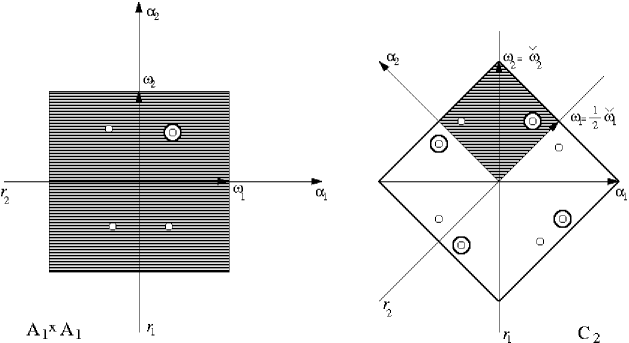
Figure 1. The simple roots, the fundamental weights, along with their dual, $\,r_{1},\,r_{2}\,$ generators of $\,W$ and the even fundamental region (shaded area) for $\mathop{\operatorname{{A_{1}}}}\nolimits\times\mathop{\operatorname{{A_{1}}}}\nolimits$ and $\mathop{\operatorname{{C_{2}}}}\nolimits$. The dots $\,\circ\,$ denote the points of $\,W$-orbit and dots $\,\bigcirc\,$ denote the points of $\,W_{e}$-orbit.

The fundamental region $F^{e}(\mathop{\operatorname{{C_{2}}}}\nolimits)$ is defined as $\,F(\mathop{\operatorname{{C_{2}}}}\nolimits)\cup r_{1}F(\mathop{\operatorname{{C_{2}}}}\nolimits)\,$, i.e.

$$F^{e}(\mathop{\operatorname{{C_{2}}}}\nolimits)=\{x\check{\omega}_{1}+y\check{\omega}_{2}\mid\text{where $0\leq y\leq 1$ and $0\leq 2x+y\leq 1$}\}.$$ (4.3)

Geometrically it is a square with vertices $0$, $\tfrac{\check{\omega}_{1}}{2}$, $\check{\omega}_{2}$ and $\check{\omega}_{2}-\tfrac{\check{\omega}_{1}}{2}$. See Figure 1 for the details.

We define $\,P_{e}=P^{+}\cup r_{1}P^{++}$. For $\lambda=(a,b)=a\omega_{1}+b\omega_{2}\in P_{e}$ the even Weyl group orbit $W_{e}(\lambda)\equiv W_{e}(a,b)$ contains either 1 or 4 points:

$$W_{e}(a,b)=\begin{cases}\{(0,0)\}&\text{if $a=b=0$,}\\ \{\pm(a,b),\pm(a+2b,-a-b)\}&\text{if\ $a^{2}+b^{2}>0$.}\end{cases}$$

According to (3.1) the $\mathop{\operatorname{{E}}}\nolimits$-functions of the Lie group $\mathop{\operatorname{{C_{2}}}}\nolimits$, with $\lambda=a\omega_{1}+b\omega_{2}$ and $z=x\check{\omega}_{1}+y\check{\omega}_{2}$, are the following

$$\begin{array}[]{l}\mathop{\operatorname{{E}}}\nolimits_{(0,0)}(x,y)=1,\\ \mathop{\operatorname{{E}}}\nolimits_{(a,b)}(x,y)=2\cos(\pi((2a+2b)x+(a+2b)y))+2\cos(\pi(2bx-ay)),\ \ \text{if \ }a^{2}+b^{2}>0\,.\end{array}$$ (4.4)

In particular, $\,\mathop{\operatorname{{E}}}\nolimits_{(a,\,0)}(x,y)=\mathop{\operatorname{{C}}}\nolimits_{(a,\,0)}(x,y)\,$ and $\,\mathop{\operatorname{{E}}}\nolimits_{(0,\,b)}(x,y)=\mathop{\operatorname{{C}}}\nolimits_{(\,0,b)}(x,y)$.

To be uniform in both formulas, we introduce a different normalization, namely,

$$\Xi_{(a,b)}(x,y)\overset{\text{\tiny def}}{=}\tfrac{|W_{e}|}{|W_{e}(a,b)|}\mathop{\operatorname{{E}}}\nolimits_{(a,b)}(x,y),$$ (4.5)

where $\,|W_{e}(a,b)|\,$ is the number of points in $\,W_{e}(a,b)$. In $\,\mathop{\operatorname{{C_{2}}}}\nolimits\,$ case we rewrite (4.4) as

$$\Xi_{(a,b)}(x,y)=2\cos(\pi((2a+2b)x+(a+2b)y))+2\cos(\pi(2bx-ay)),\quad{\rm for\ all}\ \ (a,b)\in P_{e}.$$

For any $\,(a,b),(c,d)\in P_{e}\,$, orthogonality property is verified directly,

$$\int_{F^{e}}\Xi_{(a,b)}(x,y)\overline{\Xi}_{(c,d)}(x,y)dF^{e}=\int_{0}^{1}dy\int_{-\tfrac{y}{2}}^{1-\tfrac{y}{2}}\Xi_{(a,b)}(x,y)\overline{\Xi}_{(c,d)}(x,y)dy$$

$$=\begin{cases}0,&\text{if $a\neq c$ and $b\neq d$,}\\ 2,&\text{if $a=c$ or $b=d$.}\end{cases}$$ (4.6)

In particular, we have $\,\int_{F^{e}}\Xi_{(a,b)}(x,y)dF^{e}=0\,$ for any $\,(a,b)\neq(0,0)$.

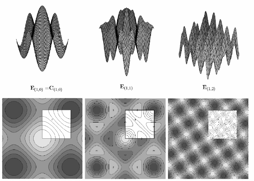
Figure 2. Examples of $\,\mathop{\operatorname{{E}}}\nolimits$-functions for $\,\mathop{\operatorname{{C_{2}}}}\nolimits.$

4.3. The $\,\mathop{\operatorname{{E}}}\nolimits$-transforms of $\mathop{\operatorname{{A_{2}}}}\nolimits$

Relative length and angles of the simple roots of $\mathop{\operatorname{{A_{2}}}}\nolimits$ are given by:

$$\langle\alpha_{1}\mid\alpha_{2}\rangle=-1,\qquad\langle\alpha_{1}\mid\alpha_{1}\rangle=\langle\alpha_{2}\mid\alpha_{2}\rangle=2.$$

Consequently,

$$\alpha_{1} =2\omega_{1}-\omega_{2}, \qquad\omega_{1} =\tfrac{1}{3}(2\alpha_{1}+\alpha_{2}),$$

$$\alpha_{2} =-\omega_{1}+2\omega_{2}, \qquad\omega_{2} =\tfrac{1}{3}(\alpha_{1}+2\alpha_{2}).$$

The root system $\Delta=\{\pm\alpha_{1},\pm\alpha_{2},\pm(\alpha_{1}+\alpha_{2})\}$ geometrically represents vertices of a regular hexagon. For details see Figure 3. Take any $\lambda=a\omega_{1}+b\omega_{2}\in P_{e}=P^{+}\cup r_{1}P^{++}$. Then the even Weyl group orbit $W_{e}(a,b)$ contains 1 or 3 points, namely

$$W_{e}(a,b)=\begin{cases}\{(0,0)\}&\text{if $a=b=0$,}\\ \{(a,b),(b,-a-b),(-a-b,a)\}&\text{if\ $a^{2}+b^{2}\neq 0.$}\\ \end{cases}$$

In particular, $\Delta=W_{(1,1)}\cup W_{(-1,-1)}$. Therefore the $\,\mathop{\operatorname{{E}}}\nolimits$-functions of $\mathop{\operatorname{{A_{2}}}}\nolimits$, with $\,\lambda=a\omega_{1}+b\omega_{2}\,$ and $\,z=x\check{\omega}_{1}+y\check{\omega}_{2}\,$, are the following:

$$\mathop{\operatorname{{E}}}\nolimits_{(0,0)}(x,y) =1,$$

$$\mathop{\operatorname{{E}}}\nolimits_{(a,b)}(x,y) =e^{\tfrac{2\pi i}{3}((2a+b)x+(a+2b)y)}+e^{-\tfrac{2\pi i}{3}((x+2y)a+(y-x)b)}+e^{-\tfrac{2\pi i}{3}((x-y)a+(2x+y)b)}.$$

In particular, $\,\mathop{\operatorname{{E}}}\nolimits_{(a,0)}(x,y)=\mathop{\operatorname{{C}}}\nolimits_{(a,0)}(x,y)\,$ and $\,\mathop{\operatorname{{E}}}\nolimits_{(0,b)}(x,y)=\mathop{\operatorname{{C}}}\nolimits_{(0,b)}(x,y)$. Using the normalization (4.5) we obtain uniform formula

$$\Xi_{(a,b)}(x,y)=e^{\tfrac{2\pi i}{3}((2a+b)x+(a+2b)y)}+e^{-\tfrac{2\pi i}{3}((x+2y)a+(y-x)b)}+e^{-\tfrac{2\pi i}{3}((x-y)a+(2x+y)b)}.$$ (4.7)

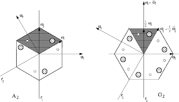
Figure 3. The simple roots, the fundamental weights, along with their dual, $\,r_{1},\,r_{2}\,$ generators of $\,W$ and the even fundamental region (shaded area) for $\mathop{\operatorname{{A_{2}}}}\nolimits$ and $\mathop{\operatorname{{G_{2}}}}\nolimits$. The dots $\,\circ\,$ denote the points of $\,W$-orbit and $\,\bigcirc\,$ the points of $W_{e}$-orbit.

The fundamental region $F^{e}(\mathop{\operatorname{{A_{2}}}}\nolimits)$ is a union of original fundamental region for Weyl group with its reflection with respect to $\,r_{1}\,$, i.e.

$$F^{e}(\mathop{\operatorname{{A_{2}}}}\nolimits)=\{x\omega_{1}+y\omega_{2}\mid\text{where $0\leq y\leq 1$ and $0\leq x+y\leq 1$}\}.$$ (4.8)

Geometrically it is a rhombus with vertices $0$, $\omega_{1}$, $\omega_{2}$ and $\omega_{2}-\omega_{1}$ (see Figure 3).

For any $\,(a,b),(c,d)\in P_{e}\,$, orthogonality property of $\,\mathop{\operatorname{{E}}}\nolimits$-functions of $\mathop{\operatorname{{A_{2}}}}\nolimits$ can be verified directly,

$$\int_{F^{e}}\Xi_{(a,b)}(x,y)\overline{\Xi}_{(c,d)}(x,y)dF^{e}=\tfrac{1}{\sqrt{3}}\int_{0}^{1}dy\int_{-y}^{1-y}\Xi_{(a,b)}(x,y)\overline{\Xi}_{(c,d)}(x,y)dy$$

$$=\begin{cases}0,&\text{if $a\neq c$ or $b\neq d$,}\\ \sqrt{3},&\text{if $a=c$ and $b=d$.}\end{cases}$$ (4.9)

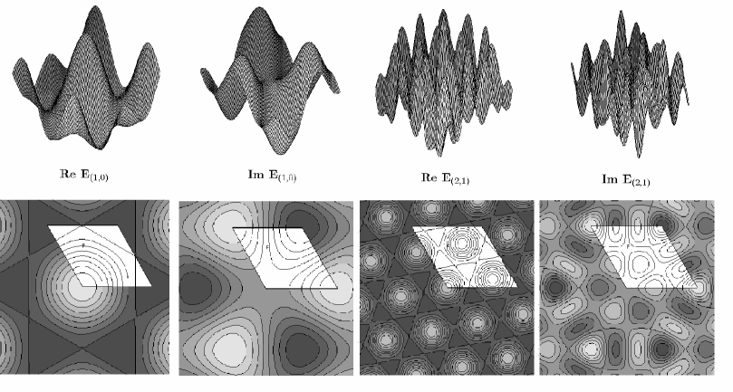
Figure 4. Real and imaginary parts of $\,\mathop{\operatorname{{E}}}\nolimits$-functions for $\,\mathop{\operatorname{{A_{2}}}}\nolimits.$

4.4. The $\mathop{\operatorname{{E}}}\nolimits$-transform of $\mathop{\operatorname{{G_{2}}}}\nolimits$

Relative length and angles of the simple roots of $\mathop{\operatorname{{G_{2}}}}\nolimits$ are given by:

$$\langle\alpha_{1}\mid\alpha_{2}\rangle=-1,\qquad\langle\alpha_{1}\mid\alpha_{1}\rangle=2,\qquad\langle\alpha_{2}\mid\alpha_{2}\rangle=\tfrac{2}{3}.$$

Then the relation between simple roots and weights is

$$\alpha_{1} =2\omega_{1}-3\omega_{2}, \qquad\omega_{1} =2\alpha_{1}+3\alpha_{2}, \qquad\check{\omega}_{1} =\omega_{1},$$

$$\alpha_{2} =-\omega_{1}+2\omega_{2}, \qquad\omega_{2} =\alpha_{1}+2\alpha_{2}, \qquad\check{\omega}_{2} =3\omega_{2}.$$

There are 12 roots in $\,\Delta(\mathop{\operatorname{{G_{2}}}}\nolimits)\,$, namely the following

$$\Delta=\{\pm(2\alpha_{1}+3\alpha_{2}),\pm(\alpha_{1}+3\alpha_{2}),\pm(\alpha_{1}+2\alpha_{2}),\pm(\alpha_{1}+\alpha_{2}),\pm\alpha_{1},\pm\alpha_{2}\}$$

geometrically the roots are vertices of a regular hexagonal star (see Figure 3).

Let $\lambda=a\omega_{1}+b\omega_{2}\in P_{e}$. Then the even Weyl group orbit $W_{e}(\lambda)\equiv W_{e}(a,b)$ contains 1 or 6 points. More precisely,

$$W_{e}(a,b)=\begin{cases}\{(0,0)\}&\text{if $a=b=0$,}\\ \{\pm(a,b),\pm(2a+b,-3a-b),\pm(-a-b,3a+2b)\}&\text{if\ $a^{2}+b^{2}\neq 0$.}\end{cases}$$

The $\,\mathop{\operatorname{{E}}}\nolimits$-functions (4.5) of $\mathop{\operatorname{{G_{2}}}}\nolimits$, with $\lambda=a\omega_{1}+b\omega_{2}$ and $z=x\check{\omega}_{1}+y\check{\omega}_{2}$, are the following:

$$\Xi_{(a,b)}(x,y) =2\cos(2\pi((2a+b)x+(3a+2b)y))+2\cos(2\pi(ax+(3a+b)y))$$ (4.10)

$$\ +2\cos(2\pi((a+b)x+by)),\quad(a,b)\in P_{e}.$$ (4.11)

The fundamental region $F^{e}(\mathop{\operatorname{{G_{2}}}}\nolimits)$ is $\,F(\mathop{\operatorname{{G_{2}}}}\nolimits)\cup r_{2}F(\mathop{\operatorname{{G_{2}}}}\nolimits)\,$:

$$F^{e}(\mathop{\operatorname{{G_{2}}}}\nolimits)=\{x\check{\omega}_{1}+y\check{\omega}_{2}\mid\text{where $0\leq x\leq 1$ and $0\leq 2x+3y\leq 1$}\}.$$

It is a triangle with vertices $0$, $\tfrac{\check{\omega}_{2}}{3}$ and $\tfrac{\check{\omega}_{1}}{2}-\tfrac{\check{\omega}_{2}}{3}$ (see Figure 3). Note that for $\,\mathop{\operatorname{{G_{2}}}}\nolimits\,$ we choose the reflection with respect to $\,r_{2}$. Therefore we also have to redefine $\,P^{e}(\mathop{\operatorname{{G_{2}}}}\nolimits)=P^{+}\cup r_{2}P^{++}$.

Orthogonality of $\,\mathop{\operatorname{{E}}}\nolimits$-functions of $\mathop{\operatorname{{G_{2}}}}\nolimits$ can be verified, for any $\,(a,b),$ $\,(c,d)\in P_{e}\,$

$$\int_{F^{e}}\Xi_{(a,b)}(x,y)\overline{\Xi}_{(c,d)}(x,y)dF^{e}=\sqrt{3}\int_{0}^{1}dx\int_{-\tfrac{2x}{3}}^{\tfrac{1-2x}{3}}\Xi_{(a,b)}(x,y)\overline{\Xi}_{(c,d)}(x,y)dy$$

$$=\begin{cases}0,&\text{if $a\neq c$ or $b\neq d$,}\\ 2\sqrt{3},&\text{if $a=c$ and $b=d$.}\\ \end{cases}$$ (4.12)

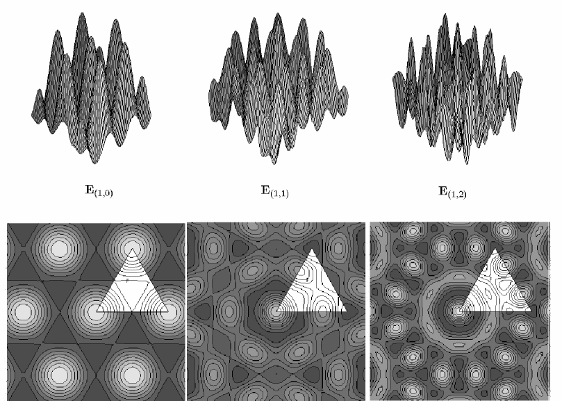
Figure 5. The $\,\mathop{\operatorname{{E}}}\nolimits$-functions for $\,\mathop{\operatorname{{G_{2}}}}\nolimits.$

5. A discrete $\,\mathop{\operatorname{{E}}}\nolimits$-function transforms

We introduce the essentials of the discrete finite $\,\mathop{\operatorname{{E}}}\nolimits$-function transform. This transform can be used, for example, to interpolate values of a function $\,f(x)\,$ between its given values on a lattice $F^{e}_{M}\subset F$. The discretization of $\,\mathop{\operatorname{{E}}}\nolimits$-functions closely parallels that of both $\,\mathop{\operatorname{{C}}}\nolimits$- and $\,\mathop{\operatorname{{S}}}\nolimits$-function, [3]-[5]. All the details of the proof for the discrete finite $\,\mathop{\operatorname{{E}}}\nolimits$-transforms are found in [2]. Recall (2.2), that the lattice $\,\check{Q}\,$ is a discrete $\,W$-invariant subset of $\,\mathbb{R}^{n}$. Then for any positive integer $\,M\,$ the set

$$T_{M}=\tfrac{1}{M}\check{Q}/\check{Q}=\bigcup_{i=1}^{n}\tfrac{d_{i}\check{\alpha}_{i}}{M},\quad d_{i}=0,\dots,M-1$$ (5.1)

is finite and $\,W$-invariant. Moreover, $\,T_{M}\,$ forms the Abelian subgroup of the maximal torus, generated by the elements of order $M$, of simple compact Lie group corresponding to $\,W$. One has the basic discrete orthogonal relation on $\,T_{M}\,$ for $\,\lambda,\,\mu\in P\,$

$$\sum_{s\in T_{M}}e^{2\pi\langle\lambda,s\rangle}\overline{e^{2\pi\langle\mu,s\rangle}}=\begin{cases}|T_{M}|,\qquad{\rm if\ \ }\lambda_{|T_{M}}=\mu_{|T_{M}},\\ 0,\qquad\text{otherwise.}\\ \end{cases}$$ (5.2)

We define the equidistant grid $\,F^{e}_{M}\,$ of points in the fundamental region $\,F^{e}$, namely

$$F^{e}_{M}\overset{\text{\tiny def}}{=}F_{M}\cup\,r_{1}(F_{M})=\{s=\tfrac{s_{1}}{M}\check{\omega}_{1}+\dots+\tfrac{s_{n}}{M}\check{\omega}_{n},\,|\,s_{i}\in\mathbb{Z}^{\geq 0},\,\sum_{i=1}^{n}s_{i}m_{i}\leq M\}\cup\{r_{1}(s)\,|\,s\in F_{M}\,\}$$ (5.3)

where $\,m_{i}$’s are the coefficients of the highest root $\,\xi_{h}$.

For any two functions $\,f$, $\,g\,$ given by their values on some $\,F^{e}_{M}\,$ we introduce a bilinear form

$$\langle f|\,g\rangle_{M}\overset{\text{\tiny def}}{=}\sum_{s\in F^{e}_{M}}\varepsilon_{s}f(s)\overline{g(s)}.$$ (5.4)

The coefficients $\,\varepsilon_{s}\,$ in the sum over $F^{e}_{M}$ are equal to the number of points in the torus $\,T_{M}\,$ that are conjugate to the point $s\in F^{e}_{M}$. By (5.2) for any $\,M\,$ positive integer there exists a finite set $\,\Lambda_{M}\,$ of $\,P_{e}\,$ such that for any two $\,\lambda,\,\lambda^{\prime}\in\Lambda_{M}\,$

$$\langle\Xi_{\lambda}|\,\Xi_{\lambda^{\prime}}\rangle_{M}=\sum_{s\in F^{e}_{M}}\varepsilon_{s}\Xi_{\lambda}(s)\overline{\Xi(s)}=\delta_{\lambda,\lambda^{\prime}}\langle\Xi_{\lambda}|\,\Xi_{\lambda}\rangle_{M}.$$ (5.5)

As a consequence of the orthogonality property (5.5), we get the following decomposition for any function $\,f(s)\,$ with known values on points of $\,F_{M}^{e}$. Indeed, if $\,f(s)\,$ is given

$$f(s)=\sum_{\Xi_{\lambda}\in\Lambda_{M}}d_{\lambda}\Xi_{\lambda}(s)$$ (5.6)

Then using the orthogonality property (5.5) we may calculate $\,d_{\lambda}\,$ as

$$d_{\lambda}=\tfrac{\,\langle f|\,\Xi_{\lambda}\rangle_{M}}{\langle\,\Xi_{\lambda}|\,\Xi_{\lambda}\rangle_{M}}$$ (5.7)

Once $\,d_{\lambda}\,$ of the original decomposition (5.6) were calculated, one can extend discrete variables in $F_{M}$ to continues ones:

$$f_{\rm cont}(x)\overset{\text{\tiny def}}{=}\sum_{\Xi_{\lambda}\in\Lambda_{M}}d_{\lambda}\Xi_{\lambda}(x).$$ (5.8)

It turns out that the function $\,f_{\rm cont}(x)\,$ smoothly interpolates the values of $f(s)$, while coinciding with it at the points of $F^{e}_{M}$.

Note that to find coefficients $\,\varepsilon_{s}\,$ one may use the corresponding $\,\mathop{\operatorname{{C}}}\nolimits$-function coefficients $\,c_{s},$ $\,s\in F_{M}$, which is equal to the number of point in $\,T_{M}\,$ that are congruent to $\,s$. Indeed, by (2.11) $\,F^{e}=F\cup r_{i}F$ for some $\,i\in\{1,\dots,n\}\,$. Then for $\,s=(s_{1},\dots,s_{n})\in F_{M}\,$

$$\varepsilon_{s}=\begin{cases}\tfrac{1}{2}c_{s},&\text{if $s_{i}\neq 0$,}\\ c_{s},&\text{if $s_{i}=0$.}\\ \end{cases}$$ (5.9)

5.1. Example: discretization of $\mathop{\operatorname{{A_{1}}}}\nolimits$

Here we give the description of the $\mathop{\operatorname{{A_{1}}}}\nolimits$ version of the discrete orthogonality of the $\,\mathop{\operatorname{{E}}}\nolimits$-functions.

First, we fix $\,M\in\mathbb{N}\,$, which determines an equidistant grid of $\,2M+1\,$ points $\,F_{M}\,$:

$$F^{e}_{M}=\{-1,-\tfrac{M-1}{M},\dots,-\tfrac{1}{M},0,\tfrac{1}{M},\tfrac{2}{M},\dots,\tfrac{M-1}{M},1\}.$$ (5.10)

The scalar product in the space of functions defined on $\,F^{e}_{M}\,$ is

$$\langle f\mid h\rangle_{M}\overset{\text{\tiny def}}{=}\sum_{s\in T_{M}}f(s)h(s)=\sum_{s\in F^{e}_{M}}c_{s}f(s)h(s).$$ (5.11)

For any $\,s\neq\pm 1\,$ there is no other point of $\,T_{M}\,$ which is conjugated to $\,s\,$ therefore $\,\varepsilon_{s}=1$. The point $\,s=1\,$ is conjugate to $\,s=-1\,$ and only one of them belongs to $\,T_{M}\,$ thus $\,\varepsilon_{-1}=\varepsilon_{1}=\tfrac{1}{2}$. Analogously to the continuous case we obtain the discrete orthogonality property of the $\,\mathop{\operatorname{{E}}}\nolimits$-functions over $F^{e}_{M}$:

$$\langle\mathop{\operatorname{{E}}}\nolimits_{m}\mid\mathop{\operatorname{{E}}}\nolimits_{m^{\prime}}\rangle_{M}=\begin{cases}2M,&\text{if $m=m^{\prime}\mod 2M$,}\\ 0,&\text{if $m\neq m^{\prime}\mod 2M$.}\\ \end{cases}$$ (5.12)

Let $f(s)$ be a function with known real values on $F_{M}$, and be decomposed as follows,

$$f(s)=\sum_{k=-M}^{M}\ d_{k}\mathop{\operatorname{{E}}}\nolimits_{k}(s),\quad s\in F^{e}_{M}.$$ (5.13)

Then we can compute the coefficients $d_{k}$ from

$$\langle f\mid\mathop{\operatorname{{E}}}\nolimits_{k}\rangle_{M}=\sum_{s\in F_{M}}\varepsilon_{s}f(s)\mathop{\operatorname{{E}}}\nolimits_{k}(s)=\begin{cases}4Md_{k},&\text{if $k=-M$ or $k=M$,}\\ 2Md_{k},&\text{if $k=-M+1,\dots,M-1$.}\end{cases}$$ (5.14)

After the coefficients $\,d_{k}\,$ have been calculated, one can replace $\,s\,$ in (5.13) by the continuous variable $\,x\,$:

$$f_{\rm cont}(x)\overset{\text{\tiny def}}{=}\sum_{k=-M}^{M}\ d_{k}\mathop{\operatorname{{E}}}\nolimits_{k}(x),\quad\text{where $x\in\mathbb{R}$.}$$ (5.15)

At $x=s\in F^{e}_{M}$, the continuous function $f_{\rm cont}(x)$ coincides with $f(s)$.

6. Discretization of two-dimensional transforms

This section contains all the details of the exploration of the method of finite $\,\mathop{\operatorname{{E}}}\nolimits$-function transform corresponding to the simple Lie groups of rank $\,2$. General structure of the discrete $\,2$-dimensional $\,\mathop{\operatorname{{E}}}\nolimits$-transform is the following: for any function $\,f\,$ given on the discrete grid $\,F^{e}_{M}\,$

$$f_{\rm cont}(x,y)=\sum_{(a,b)\in\,\Lambda_{M}}d_{(a,b)}\Xi_{(a,b)}(x,y),$$ (6.1)

$$d_{(a,b)}=\tfrac{\,\langle f|\,\Xi_{(a,b)}\rangle_{M}}{\langle\,\Xi_{(a,b)}|\,\Xi_{(a,b)}\rangle_{M}}.$$

Here $\,\langle\ ,\ \rangle_{M}\,$ denotes the Hermitian form (5.4). For the particular Lie group $\,G\,$ besides the corresponding $\,\mathop{\operatorname{{E}}}\nolimits$-functions there are four other data one needs to perform transform (6.1):

(i)  The finite grid $\,F^{e}_{M}\subset F^{e}$;

(ii)  The coefficients $\,\varepsilon_{s}\,$ for $\,s\in F^{e}_{M}\,$;

(iii) The finite subset $\,\Lambda_{M}\,$ of $\,P_{e}$;

(iv) The normalization coefficients $\,\langle\,\Xi_{(a,b)}|\,\Xi_{(a,b)}\rangle_{M}$, $\,(a,b)\in\Lambda_{M}.$

6.1. Discretization in the case of $\mathop{\operatorname{{C_{2}}}}\nolimits$

First we describe the grid $\,F^{e}_{M}\,$ as in (5.10). Since the highest root of $\,\mathop{\operatorname{{C_{2}}}}\nolimits\,$ is $\,2\alpha_{1}+\alpha_{2}\,$

$$F^{e}_{M}\overset{\text{\tiny def}}{=}\left\{\left(\tfrac{s_{1}}{M},\tfrac{s_{2}}{M}\right)\mid s_{0},s_{1},s_{2}\in\mathbb{Z}^{\geq 0},\quad s_{0}+2s_{1}+s_{2}=M>0\right\}\cup\left\{\left(\tfrac{-s_{1}}{M},\tfrac{s_{2}+2s_{1}}{M}\right)\mid s_{2}\neq 0\right\}.$$

See Figure 6 for $\,F^{e}_{M}$, $\,M=3,\,4$.

The coefficients $\,c_{s}\,$ for $\,\mathop{\operatorname{{C_{2}}}}\nolimits\,$ are found in [3]. By (5.9)

$$\varepsilon_{s}\equiv\varepsilon_{\left(\tfrac{s_{1}}{M},\tfrac{s_{2}}{M}\right)}=\begin{cases}1,&\text{if $s_{1}=0$ and $s_{2}=0,M$,}\\ &\text{or $s_{2}=0$ and $s_{1}=\tfrac{M}{2}$,}\\ &\text{or $s_{1}=-\tfrac{M}{2}$ and $s_{2}=M$,}\\ 2,&\text{if $2s_{1}+s_{2}=0$ and $0<s_{2}<M$,}\\ &\text{or $2s_{1}+s_{2}=M$ and $0<s_{2}<M$,}\\ &\text{or $s_{2}=0$ and $0<s_{1}<\tfrac{M}{2}$,}\\ &\text{or $s_{2}=M$ and $-\tfrac{M}{2}<s_{1}<0$,}\\ 4&\text{if $0<s_{2}<M$ and $0<2s_{1}+s_{2}<M$.}\end{cases}$$ (6.2)

The finite set $\,\Lambda_{M}=\{(a,b)\in P_{e}\,|\,0<a+2b\leq M,\,0\leq a<M\}$. Then for any $\,(a,b)\neq(a^{\prime},b^{\prime})\in\Lambda_{M}\,$

$$\langle\Xi_{(a,b)}\mid\Xi_{(a^{\prime},b^{\prime})}\rangle_{M}=0,$$

otherwise, for the set of the lowest pairwise orthogonal normalized $\,\Xi$-functions:

$$\langle\Xi_{(a,b)}\mid\Xi_{(a,b)}\rangle_{M}=8M^{2}\times\begin{cases}4,&\text{if $\,a=0,\,M\,$ and $\,b=0$,}\\ 2,&\text{if $\,a=0\,$ and $\,b=\tfrac{M}{2}$,}\\ 1,&\text{if $\,0<a<M\,$ and $\,0<a+2b<M$,}\\ &\text{or $\,a=0\,$ and $\,0<b<\tfrac{M}{2}$,}\\ &\text{or $\,a+2b=M\,$ and $\,0<b<\tfrac{M}{2}$}.\end{cases}$$

with the higher $\,\Xi$-functions repeating the values of the lowest ones.

Figure 6. The lattice points of $\,F^{e}_{3},\,F^{e}_{4}\,$ in the fundamental region $\,F^{e}\,$ for $\,\mathop{\operatorname{{C_{2}}}}\nolimits\,$ and $\,\mathop{\operatorname{{A_{2}}}}\nolimits.$

6.2. Discretization in the case of $\mathop{\operatorname{{A_{2}}}}\nolimits$

First we describe the grid $\,F^{e}_{M}\,$ as in (5.10). The highest root of $\,\mathop{\operatorname{{A_{2}}}}\nolimits\,$ is $\,\alpha_{1}+\alpha_{2},$ therefore

$$F^{e}_{M}\overset{\text{\tiny def}}{=}\left\{\left(\tfrac{s_{1}}{M},\tfrac{s_{2}}{M}\right)\mid s_{0},s_{1},s_{2}\in\mathbb{Z}^{\geq 0},\quad s_{0}+s_{1}+s_{2}=M>0\right\}\cup\left\{\left(\tfrac{-s_{1}}{M},\tfrac{s_{2}+s_{1}}{M}\right)\mid s_{1}\geq 0\right\}.$$

See Figure 6 for $\,F^{e}_{M}$, $\,M=3,\,4$.

The coefficients $\,c_{s}\,$ for $\,\mathop{\operatorname{{A_{2}}}}\nolimits\,$ are found in [4]. By (5.9)

$$\varepsilon_{s}\equiv\varepsilon_{\left(\tfrac{s_{1}}{M},\tfrac{s_{2}}{M}\right)}=\begin{cases}\tfrac{1}{2}&\text{if $\,s_{2}=0\,$ and $\,s_{1}=M$,}\\ &\text{or $\,s_{2}=M\,$ and $\,s_{1}=-M$,}\\ 1,&\text{if $\,s_{1}=0\,$ and $\,s_{2}=0,M$,}\\ \tfrac{3}{2},&\text{if $\,s_{2}=0\,$ and $\,0<s_{1}<M$,}\\ &\text{or $\,s_{2}=M\,$ and $\,-M<s_{1}<0$,}\\ &\text{or $\,s_{1}+s_{2}=M\,$ and $\,0<s_{2}<M$,}\\ &\text{or $\,s_{1}+s_{2}=0\,$ and $\,0<s_{2}<M$,}\\ 3,&\text{if $\,0<s_{2}<M\,$ and $\,0<s_{1}+s_{2}<M$.}\end{cases}$$ (6.3)

The finite set $\,\Lambda_{M}=\{(a,b)\in P_{e}\,|\,0<a+b\leq M,\,0\leq a<M\}$. For any $\,(a,b)\neq(a^{\prime},b^{\prime})\in\Lambda_{M}\,$

$$\langle\Xi_{(a,b)}\mid\Xi_{(a^{\prime},b^{\prime})}\rangle_{M}=0,$$

otherwise, for the set of the lowest pairwise orthogonal normalized $\Xi$-functions:

$$\langle\Xi_{(a,b)}\mid\Xi_{(a,b)}\rangle_{M}=9M^{2}\times\begin{cases}1,&\text{if $0<a<M$ and $b=0,M$,}\\ &\text{if $0\leq a+b\leq M$ and $0<a<M$,}\\ 3,&\text{if $a=0$ and $b=0$,}\\ &\text{or $a=0$ and $b=M$,}\\ &\text{or $a=M$ and $b=0$.}\end{cases}$$

with the higher $\Xi$-functions repeating the values of the lowest ones.

6.3. Discretization in the case of $\mathop{\operatorname{{G_{2}}}}\nolimits$

Since the highest root of $\,\mathop{\operatorname{{G_{2}}}}\nolimits\,$ is $\,2\alpha_{1}+3\alpha_{2}\,$ the grid $\,F^{e}_{M}\,$ is

$$F^{e}_{M}\overset{\text{\tiny def}}{=}\left\{\left(\tfrac{s_{1}}{M},\tfrac{s_{2}}{M}\right)\mid s_{0},s_{1},s_{2}\in\mathbb{Z}^{\geq 0},\quad s_{0}+2s_{1}+3s_{2}=M>0\right\}\cup\left\{\left(\tfrac{2s_{1}+3s_{2}}{M},\tfrac{-s_{2}}{M}\right)\mid s_{2}\geq 0\right\}.$$

The coefficients $\,c_{s}\,$ for $\,\mathop{\operatorname{{G_{2}}}}\nolimits\,$ are found in [3]. By (5.9)

$$\varepsilon_{s}\equiv\varepsilon_{\left(\tfrac{s_{1}}{M},\tfrac{s_{2}}{M}\right)}=\begin{cases}1,&\text{if $s_{1}=0$ and $s_{2}=0$,}\\ &\text{or $s_{1}=0$ and $s_{2}=\tfrac{M}{3}$,}\\ &\text{or $s_{1}=M$ and $s_{2}=-\tfrac{M}{3}$,}\\ 3,&\text{if $s_{1}=0$ and $0<s_{2}<\tfrac{M}{3}$,}\\ &\text{or $3s_{2}+s_{1}=0$ and $0<s_{1}<M$,}\\ &\text{or $3s_{2}+2s_{1}=M$ and $0<s_{1}<M$,}\\ 6,&\text{if $0<s_{1}<M$ and $0<s_{1}+3s_{2}$ and $2s_{1}+3s_{2}<M$.}\end{cases}$$ (6.4)

The finite set $\,\Lambda_{M}=\{(a,b)\in P_{e}\,|\,0<3a+b,\ 3a+2b\leq M,\,0\leq a\leq\tfrac{M}{3}\}$. Then for any $\,(a,b)\neq(a^{\prime},b^{\prime})\in\Lambda_{M}\,$

$$\langle\mathop{\operatorname{{E}}}\nolimits_{(a,b)}\mid\mathop{\operatorname{{E}}}\nolimits_{(a^{\prime},b^{\prime})}\rangle_{M}=0,$$

otherwise, for the set of the lowest pairwise orthogonal normalized $\,\mathop{\operatorname{{E}}}\nolimits$-functions:

$$\langle\mathop{\operatorname{{E}}}\nolimits_{(a,b)}\mid\mathop{\operatorname{{E}}}\nolimits_{(a,b)}\rangle_{M}=6M^{2}\times\begin{cases}6,&\text{if $\,a=0\,$ and $\,b=0$,}\\ 3,&\text{if $\,a=\tfrac{M}{3}\,$ and $\,b=0$,}\\ 2,&\text{if $\,a=0\,$ and $\,b=\tfrac{M}{2}$,}\\ 1,&\text{or $b=0$ and $0<3a<M$,}\\ &\text{if $a=0$ and $0<2b<M$,}\\ &\text{or $0<3a+b$ and $3a+2b<M$.}\\ \end{cases}$$

with the higher $\,\mathop{\operatorname{{E}}}\nolimits$-functions repeating the values of the lowest ones.

7. Decomposition of products of $\,\mathop{\operatorname{{E}}}\nolimits$-functions

For any two points $\,\lambda,\,\lambda^{\prime}\in P_{e}\,$ define the product of corresponding orbits $\,W_{e}(\lambda)\otimes W_{e}(\lambda^{\prime})\,$ as a set of all points in $\,\mathbb{R}^{n}\,$ of the form $\,\mu+\mu^{\prime}$, $\mu\in W_{e}(\lambda)$, $\,\mu^{\prime}\in W_{e}(\lambda^{\prime})$. Since the set of the points $\,\mu+\mu^{\prime}\,$ $\,\mu\in W_{e}(\lambda)$, $\,\mu^{\prime}\in W_{e}(\lambda^{\prime})\,$ is invariant under the action of corresponding even Weyl group, for any $\,\gamma\in W_{e}(\lambda)\otimes W_{e}(\lambda^{\prime})\,$ we obtain that

$$\,W_{e}(\gamma)\subset W_{e}(\lambda)\otimes W_{e}(\lambda^{\prime}).$$ (7.1)

Therefore any product of two orbits can be seen as a union of finite number of orbits of $\,W_{e}$.

Let both $\,\lambda\,$ and $\,\lambda^{\prime}\,$ be in $\,P_{e}\,$ and

$$W_{e}(\lambda)\otimes W_{e}(\lambda^{\prime})=\bigcup_{\gamma\in\,I}W_{e}(\gamma),$$ (7.2)

where $\,I\,$ is a finite subset of $\,P_{e}$. Then for the product of corresponding $\,\mathop{\operatorname{{E}}}\nolimits$-functions we have

$$\mathop{\operatorname{{E}}}\nolimits_{\lambda}(x)\mathop{\operatorname{{E}}}\nolimits_{\lambda^{\prime}}(x)=\sum_{\gamma\in\,I}\mathop{\operatorname{{E}}}\nolimits_{\gamma}(x).$$ (7.3)

Indeed, by (7.2)

$$\mathop{\operatorname{{E}}}\nolimits_{\lambda}(x)\mathop{\operatorname{{E}}}\nolimits_{\lambda^{\prime}}(x)=\sum_{\mu\in W_{e}(\lambda)}e^{2\pi i\langle\mu,\,x\rangle}\sum_{\mu^{\prime}\in W_{e}(\lambda^{\prime})}e^{2\pi i\langle\mu^{\prime},\,x\rangle}=\sum_{\gamma\in\,I}\sum_{o(\gamma)\in W_{e}(\gamma)}e^{2\pi i\langle o(\gamma),\,x\rangle}=\sum_{\gamma\in\,I}\mathop{\operatorname{{E}}}\nolimits_{\gamma}(x).$$

For the $\,\mathop{\operatorname{{E}}}\nolimits$-functions of $\,\mathop{\operatorname{{A_{1}}}}\nolimits\,$ the product decomposition was shown in (3.9). However, in higher dimensions of Euclidean spaces the problem of finding terms of the sum and their multiplicities in (7.3) is a not simple task. Further in this section we deal with decomposition of the product of $\,\mathop{\operatorname{{E}}}\nolimits$-functions for the three simple Lie groups of rank two.

7.1. Decomposition of products of $\,\mathop{\operatorname{{E}}}\nolimits$-functions for $\,\mathop{\operatorname{{C_{2}}}}\nolimits\,$

For any $\,(a,b),(c,d)\in P_{e}\$ the product in (7.3) can be written as

$$\Xi_{(a,b)}\Xi_{(c,d)}=\Xi_{(a+c,b+d)}+\Xi_{(a-c,b-d)}+\Xi_{(a+2d+c,b-c-d)}+\Xi_{(a-2d-c,b+d+c)}=\sum_{\mu\in W_{e}(c,d)}\Xi_{(a,b)+\mu}\,$$ (7.4)

Here we again we use the normalization (4.5). Moreover we can obtain analogous product decomposition rules for $\,\mathop{\operatorname{{C}}}\nolimits$-function of the Lie group $\,\mathop{\operatorname{{C_{2}}}}\nolimits\,$. For that we first introduce analogous renormalization of orbit functions. Namely,

$$\Omega_{\lambda}(x)=\frac{|W|}{|W(\lambda)|}\mathop{\operatorname{{C}}}\nolimits_{\lambda}(x).$$ (7.5)

Then from (3.4) we obtain

$$\Omega_{(a,0)} =\Xi_{(a,0)},\quad\Omega_{(0,b)}=\Xi_{(0,b)}\,,\qquad\,a,b\neq 0\,,$$ (7.6)

$$\Omega_{(a,b)} =\Xi_{(a,b)}+\Xi_{(-a,a+b)}.$$

Combining both (7.6) and (7.4) we obtain the formulas for the product of $\,\mathop{\operatorname{{C}}}\nolimits$-functions. If $\,(a,b)\in P^{++}\,$ and $\,(c,d)\in P^{+}\setminus(0,0)\,$

$$\Omega_{(a,b)}\Omega_{(c,d)}=\sum_{\mu\in W(c,d)}\tfrac{|W|}{|W((a,b)+\mu)|}\Omega_{(a,b)+\mu}.$$ (7.7)

The product of two $\,\mathop{\operatorname{{C}}}\nolimits$-functions determined by points $\,(a,b)\,$ and $\,(c,d)\,$ is decomposed into the sum of $\,\mathop{\operatorname{{C}}}\nolimits$-function labeled by weights from $\,(a,b)+W(c,d)$. In particular, if both $\,(c,d)\,$ and all the points of $\,(a,b)+W(c,d)\,$ are in $\,P^{++}\,$, we obtain

$$\Omega_{(a,b)}\Omega_{(c,d)} =\Omega_{(a+c,b+d)}+\Omega_{(a-c,b-d)}+\Omega_{(-a+c,a+b+d)}+\Omega_{(-a-c,a+b-d)}$$

$$+\Omega_{(a+c+2d,b-d)}+\Omega_{(a+c-2d,b+c+d)}+\Omega_{(a+c+2d,b-c-d)}+\Omega_{(a-c-2d,b+d)}.$$

The remaining case are

$$\Omega_{(a,0)}\Omega_{(c,0)}=\Omega_{(a+c,0)}+\Omega_{(a-c,0)}+\tfrac{|W|}{|W(a-c,c)|}\Omega_{(a-c,c)},\qquad\qquad\$$

$$\Omega_{(0,b)}\Omega_{(0,d)}=\Omega_{(0,b+d)}+\Omega_{(0,b-d)}+\tfrac{|W|}{|W(2d,b-d)|}\Omega_{(2d,b-d)},\qquad\qquad$$

$$\Omega_{(a,0)}\Omega_{(0,d)}=\tfrac{|W|}{|W(a,d)|}\Omega_{(a,d)}+\tfrac{|W|}{|W(a,-d)|}\Omega_{(a,-d)}.\qquad\qquad$$

We also can use these formulas to generalize formulas for tensor product of $\,W$-orbits of $\,\mathop{\operatorname{{C_{2}}}}\nolimits\,$ from section 4.2 in [6].

7.2. Decomposition of products of $\,\mathop{\operatorname{{E}}}\nolimits$-functions for $\,\mathop{\operatorname{{A_{2}}}}\nolimits$

Analogously to the case of $\,\mathop{\operatorname{{C_{2}}}}\nolimits\,$ group products of the $\,\mathop{\operatorname{{E}}}\nolimits$-functions of $\mathop{\operatorname{{A_{2}}}}\nolimits$ decompose into sums of $\,\mathop{\operatorname{{E}}}\nolimits$-functions. For any $\,(a,b),(c,d)\in P_{e}\,$ we obtain

$$\Xi_{(a,b)}\Xi_{(c,d)}=\Xi_{(a+c,b+d)}+\Xi_{(a+d,b-c-d)}+\Xi_{(a-c-d,b+c)}=\sum_{\mu\in W_{e}(c,d)}\Xi_{(a,b)+\mu}.$$ (7.8)

The relation (3.4) between $\,\mathop{\operatorname{{E}}}\nolimits$- and $\,\mathop{\operatorname{{C}}}\nolimits$-functions for $\,\mathop{\operatorname{{A_{2}}}}\nolimits\,$ is the following

$$\Omega_{(a,0)}=\Xi_{(a,0)},\,\quad\Omega_{(0,b)}=\Xi_{(0,b)}$$ (7.9)

$$\Omega_{(a,b)}=\Xi_{(a,b)}+\Xi_{(-a,a+b)}.$$

Here we used the normalization (7.5) for $\,\mathop{\operatorname{{C}}}\nolimits$-functions. Combining the last two formulas we obtain for any $\,(a,b)\in P^{++}\,$ and any $\,(c,d)\in P^{+}\setminus(0,0)\,$

$$\Omega_{(a,b)}\Omega_{(c,d)}=\sum_{\mu\in W(c,d)}\tfrac{|W|}{|W((a,b)+\mu)|}\Omega_{(a,b)+\mu}.$$ (7.10)

The remaining cases:

$$\Omega_{(a,0)}\Omega_{(c,0)}=\Omega_{(a+c,0)}+\tfrac{|W|}{|W(a,-c)|}\Omega_{(a,-c)},\qquad\qquad$$

$$\Omega_{(0,b)}\Omega_{(0,d)}=\Omega_{(0,b+d)}+\tfrac{|W|}{|W(-d,b)|}\Omega_{(-d,b)},\qquad\qquad$$

$$\Omega_{(a,0)}\Omega_{(0,d)}=\tfrac{|W|}{|W(a,d)|}\Omega_{(a,d)}+\Omega_{(0,-a+d)}.\qquad\qquad$$

Also we have obtained the formulas generalizing formulas for tensor product of $\,W$-orbits of $\,\mathop{\operatorname{{A_{2}}}}\nolimits\,$ from section 4.2 in [6].

7.3. Decomposition of products of $\,\mathop{\operatorname{{E}}}\nolimits$-functions for $\,\mathop{\operatorname{{G_{2}}}}\nolimits$

The products of the $\,\mathop{\operatorname{{E}}}\nolimits$-functions decompose into sums of $\,\mathop{\operatorname{{E}}}\nolimits$-functions. Namely, if $\,(a,b),\,(c,d)\in P_{e}\,$

$$\Xi_{(a,b)}\Xi_{(c,d)}=\sum_{\mu\in W_{e}(c,d)}\Xi_{(a,b)+\mu(c,d)}=\Xi_{(a+c,b+d)}+\Xi_{(a-c,b-d)}+\Xi_{(a+2d+c,b-3c-d)}$$ (7.11)

$$+\Xi_{(a-2d-c,b+3c+d)}+\Xi_{(a-c-d,b+3c+2d)}+\Xi_{(a+c+d,b-3c-2d)}.$$

In case of $\,\mathop{\operatorname{{G_{2}}}}\nolimits\,$ (3.4) gives

$$\Omega_{(a,0)}=\Xi_{(a,0)},\,\qquad\Omega_{(0,b)}=\Xi_{(0,b)}$$ (7.12)

$$\Omega_{(a,b)}=\Xi_{(a,b)}+\Xi_{(-a,3a+b)}.$$

As a sequence from (7.11) and(7.12) we obtain the decomposition for the product of $\,\Omega\,$ for $\,(a,b)\in P^{++}\,$ and $\,(c,d)\in P^{+}\setminus(0,0)$

$$\Omega_{(a,b)}\Omega_{(c,d)}=\sum_{\mu\in W(c,d)}\tfrac{|W|}{|W((a,b)+\mu)|}\Omega_{(a,b)+\mu}.$$ (7.13)

8. Central splitting for $\,\mathop{\operatorname{{E}}}\nolimits$-transforms

The idea of the central splitting of a function $f(x)$ on $F$, or $F^{e}$, of a compact semisimple Lie group $G$, is the decomposition of $f(x)$ into the sum of several component-functions, as many as is the order $\,s$ of the center $\,Z\,$ of $G$. Motivation for considering such splitting is in the property of the component-functions [2]: their $\,\mathop{\operatorname{{E}}}\nolimits$-transforms employ mutually exclusive subsets of $\,\mathop{\operatorname{{E}}}\nolimits$-functions of $G$. The functions $\,\mathop{\operatorname{{E}}}\nolimits_{\lambda}\,$ and $\,\mathop{\operatorname{{E}}}\nolimits_{\lambda^{\prime}}\,$ belong to the same subset precisely if $\,\lambda\,$ and $\,\lambda^{\prime}\,$ belong to the same congruence class.

Let $\,\chi_{1},\dots,\chi_{s}\,$ be the irreducible characters of $\,Z$. Also any $\,\lambda\in P_{e}\,$ determines an irreducible character of $\,Z$

$$\chi_{\lambda}\,:\check{z}\mapsto e^{2\pi i\langle\lambda,\check{z}\rangle}\qquad\check{z}\in Z.$$ (8.1)

Then $\,\chi_{\lambda}=\chi_{j}$ for some $\,1\leq j\leq s$. Then $\,j\,$ is called the congruence class of $\,\lambda$. It is constant on the $\,W_{e}$-orbit of $\,\lambda\,$ and therefore

$$\mathop{\operatorname{{E}}}\nolimits_{\lambda}(x+\check{z})=\chi_{j}(\check{z})\mathop{\operatorname{{E}}}\nolimits_{\lambda}(x)\qquad\check{z}\in Z.$$ (8.2)

Thus any $\,f\,$ which is linear combination of $\,\mathop{\operatorname{{E}}}\nolimits$-functions can be written as a sum of $\,s\,$ functions $\,f(x)=f_{1}+\dots+f_{s}$, where

$$f_{i}(x)=\tfrac{1}{s}\sum_{\check{z}\in Z}\overline{\chi_{i}(\check{z})}f(x+\check{z})\qquad 1\leq i\leq s.$$ (8.3)

There are two rank-two compact simple Lie groups with non-trivial center of orders $\,2$ and $\,3$, namely $\,\mathop{\operatorname{{C_{2}}}}\nolimits$ and $\,\mathop{\operatorname{{A_{2}}}}\nolimits$ respectively. The center of $\,\mathop{\operatorname{{G_{2}}}}\nolimits\,$ is trivial.

8.1. Central splitting for $\,\mathop{\operatorname{{C_{2}}}}\nolimits\,$

As we have already seen in (4.3) the fundamental region of $\,\mathop{\operatorname{{C_{2}}}}\nolimits\,$ is a square with vertices $0$, $\tfrac{\check{\omega}_{1}}{2}$, $\check{\omega}_{2}$ and $\check{\omega}_{2}-\tfrac{\check{\omega}_{1}}{2}.$ The center $\,Z\,$ has two elements $\,\{0,\check{\omega}_{2}\}$. According to [2] any function $\,f\,$ on $\,F^{e}\,$ we may decompose it into $\,f(x)=f_{0}(x)+f_{1}(x)$, where

$$f_{0}(x)=\tfrac{1}{2}\{f(x)+f(x+\check{\omega}_{2})\}\quad{\rm and}\quad f_{1}(x)=\tfrac{1}{2}\{f(x)-f(x+\check{\omega}_{2})\}.$$ (8.4)

However for any $\,x=a\check{\omega}_{1}+b\check{\omega}_{2}\in F^{e}\,$ the point $\,x+\check{\omega}_{2}\,$ is outside of $\,F^{e}$. By suitable transformation we bring it back to the fundamental region:

$$r_{\alpha_{2},1}r_{\alpha_{1}}r_{\alpha_{2},1}r_{\alpha_{1}}(a,b+1)=(-a,1-b).$$

Therefore the component function can be written for $\,x\,$ in $\,\check{\omega}$-basis as

$$\begin{array}[]{c}f_{0}(a,b)=\tfrac{1}{2}\{f(a,b)+f(-a,1-b)\}\\ f_{1}(a,b)=\tfrac{1}{2}\{f(a,b)-f(-a,1-b)\}.\end{array}$$

The main property of both $\,f_{0}\,$ and $\,f_{1}\,$ is that each of them decomposes into a linear combination of $\,\mathop{\operatorname{{E}}}\nolimits$-functions from one congruence class only $\,0\,$ for $\,f_{0}\,$ and $\,1\,$ for $\,f_{1}$.

8.2. Central splitting for $\,\mathop{\operatorname{{A_{2}}}}\nolimits\,$

In the case of $\,\mathop{\operatorname{{A_{2}}}}\nolimits\,$ the fundamental region is a rhombus with vertices $0$, $\omega_{1}$, $\omega_{2}$ and $\omega_{2}-\omega_{1}$ as in (4.8). The center $\,Z\,$ has three elements $\,\{0,{\omega}_{1},{\omega}_{2}\}\,$ and any function on $\,F^{e}\,$ is decomposed into the sum of three function $\,f(x)=f_{0}(x)+f_{1}(x)+f_{2}(x)\,$ where

$$\begin{array}[]{l}f_{0}(x)=\tfrac{1}{3}\{f(x)+f(x+{\omega}_{1})+f(x+{\omega}_{2})\},\\ f_{1}(x)=\tfrac{1}{3}\{f(x)+e^{-2\pi i/3}f(x+{\omega}_{1})+e^{-2\pi i/3}f(x+{\omega}_{2})\},\\ f_{2}(x)=\tfrac{1}{3}\{f(x)+e^{2\pi i/3}f(x+{\omega}_{1})+e^{2\pi i/3}f(x+{\omega}_{2})\}.\end{array}$$

Again for $\,x=a{\omega}_{1}+b{\omega}_{2}\in F^{e}\,$ both $\,x+{\omega}_{1}\,$ and $\,x+{\omega}_{2}\,$ are not necessarily in $\,F^{e}$. We have $\,x+{\omega}_{1}=(a+1,b)\,$ and $\,x+{\omega}_{2}=(a,b+1)$. Then there are two cases for points $\,(a,b+1)\,$ and $\,(a+1,b)\,$ to be brought to $\,F^{e}$ by suitable transformations from the affine Weyl group of $\,\mathop{\operatorname{{A_{2}}}}\nolimits$.

$$\begin{array}[]{c}r_{\alpha_{2},1}r_{\alpha_{1}}(a,b+1)=(b,-a-b+1)\\ r_{\alpha_{1},1}r_{\alpha_{2}}(a+1,b)=(1-a-b,a)\end{array}\quad{\rm for}\ a\geq 0$$

and

$$\begin{array}[]{c}r_{\alpha_{1}}r_{\alpha_{2},1}(a,b+1)=(b-1,a+1)\\ r_{\alpha_{2},1}r_{\alpha_{1}}(a+1,b)=(b-1,-a-b+1)\end{array}\quad{\rm for}\ a<0.$$

Finally, one obtains, for $\,x=(a,b)\in F^{e}$, $\,a\geq 0$

$$\begin{array}[]{c}f_{0}(a,b)=\tfrac{1}{3}\{f(a,b)+f(b-1,-a-b+1)+f(b-1,a+1)\}\\ f_{1}(a,b)=\tfrac{1}{3}\{f(a,b)+e^{-2\pi i/3}f(b-1,-a-b+1)+e^{-2\pi i/3}f(b-1,a+1)\},\\ f_{2}(a,b)=\tfrac{1}{3}\{f(a,b)+e^{2\pi i/3}f(b-1,-a-b+1)+e^{2\pi i/3}f(b-1,a+1)\}\end{array}$$

or if $\,x=(a,b)\in F^{e}$, $\,a<0\,$

$$\begin{array}[]{c}f_{0}(a,b)=\tfrac{1}{3}\{f(a,b)+f(1-a-b,a)+f(b,-a-b+1)\}\\ f_{1}(a,b)=\tfrac{1}{3}\{f(a,b)+e^{-2\pi i/3}f(1-a-b,a)+e^{-2\pi i/3}f(b,-a-b+1)\},\\ f_{2}(a,b)=\tfrac{1}{3}\{f(a,b)+e^{2\pi i/3}f(1-a-b,a)+e^{2\pi i/3}f(b,-a-b+1)\}.\end{array}$$

Again each $\,f_{i},$ $\,i=0,1,2\,$ in this sum may be decomposed as a sum of $\,\mathop{\operatorname{{E}}}\nolimits$-functions from the congruence class $\,i$.

9. Concluding remarks

1. Similarly as the $\mathop{\operatorname{{C}}}\nolimits$- and $\mathop{\operatorname{{S}}}\nolimits$-functions, the $\,\mathop{\operatorname{{E}}}\nolimits$-functions can be viewed as a family of orthogonal polynomials, related to a particular semisimple Lie group and to a particular $W_{e}$-orbit, in as many variables as is the rank of the group. Such variables, as we use them here, are constrained to the $n$-dimensional torus of the appropriate Lie group. The polynomials have many properties of traditional special functions. Easy discretization of the polynomials is an unusual feature, particularly in a multidimensional set up.

2.  The $\,\mathop{\operatorname{{E}}}\nolimits$-functions of $\,\mathop{\operatorname{{SU}}}\nolimits(2)\,$ are common exponential function in one variable

$$\mathop{\operatorname{{E}}}\nolimits_{m}(x)=e^{imx}=\tfrac{1}{2}(\mathop{\operatorname{{C}}}\nolimits_{m}(x)+\mathop{\operatorname{{S}}}\nolimits_{m}(x)).$$

Roughly speaking, $\,\mathop{\operatorname{{E}}}\nolimits$-function are related to $\,\mathop{\operatorname{{C}}}\nolimits$- and $\,\mathop{\operatorname{{S}}}\nolimits$-functions as the exponential function is related to cosine and sine functions. The special role of imaginary unit does not seem to generalize.

3.  Besides three introduced transforms in the case when $\,G\,$ is semisimple there are other derived transforms which may be considered. Suppose $\,G=G_{1}\times G_{2}$, where $\,G_{1}\,$ and $\,G_{2}$. Let $\,F_{1}\,$ be either the fundamental region of $\,G_{1}\,$ or fundamental region of its even subgroup and $\,F_{2}\,$ respectively for $\,G_{2}$. Then any function $\,f(x_{1},x_{2})\,$ on $\,F_{1}\times F_{2}\,$ can be expanded using any of $\,\mathop{\operatorname{{C}}}\nolimits$- $\,\mathop{\operatorname{{S}}}\nolimits$-, $\,\mathop{\operatorname{{E}}}\nolimits$-functions on $\,F_{1}\,$ and any of these three types on $\,F_{2}$. Thus one may have $\,\mathop{\operatorname{{E}}}\nolimits\mathop{\operatorname{{C}}}\nolimits$ or $\,\mathop{\operatorname{{S}}}\nolimits\mathop{\operatorname{{E}}}\nolimits$-transforms rather then $\,\mathop{\operatorname{{E}}}\nolimits\mathop{\operatorname{{E}}}\nolimits$-transforms we studied in the main body of the paper.

4.  The $\mathop{\operatorname{{E}}}\nolimits$-functions are complex valued, in general. A function $\mathop{\operatorname{{E}}}\nolimits_{\lambda}(x)$ is real precisely if the orbit $W_{e}(\lambda)$ contains both weights $\pm\lambda$. More about when that happens see in [2].

5.   A choice of $\,W_{e}^{\rm aff}$-fundamental domain $F^{e}$ is not unique. It is made out of two adjacent copies of the fundamental domain $F$ of $W$. One can flip $F$ in any of its $(n-1)$dimensional faces in order to get $F^{e}$. Obviously, for any choice of $\,F^{e}\,$ one can introduce both continuous and discrete transform: general theory allows one to set up $\,P_{e}$, $\,F^{e}_{M}$ etc. It is conceivable that practical considerations may dictate preferred choice.

6.  As we already mentioned in the introduction there are two ways to define even Weyl group in case when original Lie group is a product of two simple Lie groups $\,G=G_{1}\times G_{2}$. First possibility is when $\mathop{\operatorname{{E}}}\nolimits$-transform of $G$ is taken up to be the simultaneous $\mathop{\operatorname{{E}}}\nolimits$-transform of $G_{1}$ and the $\mathop{\operatorname{{E}}}\nolimits$-transform of $G_{2}$. The $\mathop{\operatorname{{E}}}\nolimits$-functions of $G$ are products of $\mathop{\operatorname{{E}}}\nolimits$-functions of $G_{1}$ and the $\mathop{\operatorname{{E}}}\nolimits$-functions of $G_{2}$. In this case we take $W_{e}(G)$ to be $W_{e}(G_{1})\times W_{e}(G_{2})$.

The second possibility arises from the fact that

$$W_{e}(G_{1}\times G_{2})\neq W_{e}(G_{1})\times W_{e}(G_{2}).$$ (9.1)

Consider for example $G=\mathop{\operatorname{{SU}}}\nolimits(2)\times\mathop{\operatorname{{SU}}}\nolimits(2)$. Its Weyl group is of order four, its elements being $1,\ r_{1},\ r_{2},\ r_{1}r_{2}$. Hence $W_{e}(\mathop{\operatorname{{SU}}}\nolimits(2)\times\mathop{\operatorname{{SU}}}\nolimits(2))$ has two elements, namely $1$ and $r_{1}r_{2}$. In three dimensions the possibilities this option allows are more curious, interesting and involved. We are going to pursue them elsewhere.

7.   The most important qualitative argument in favor of efficiency of discrete and continuous expansions of functions given on $F$ into series of either $\mathop{\operatorname{{C}}}\nolimits$- or $\mathop{\operatorname{{S}}}\nolimits$- or $\mathop{\operatorname{{E}}}\nolimits$-functions, is that they involve discrete groups larger than the translation group of traditional Fourier expansions. Indeed, it is the affine Weyl group acting in $\mathbb{R}^{n}$, which contains the translations as its subgroup. More specifically, the fundamental region of the translation group is the proximity cell (Voronoi domain) $V$ of the root lattice of $G$, while the fundamental region $F$ for the affine Weyl group is much smaller, $|V|=|F||W|$. Thus the larger is is the order $|W|$ of the Weyl group, the more efficient are our expansions (fewer ‘harmonics’ needed). The Voronoi domains of root lattices for all simple $G$ are described in [14].

Independently interesting would be to study multidimensional Fourier expansions in general, that is expansions based on translational symmetry, as opposed the reflection symmetry of the affine Weyl group we use. In that case Voronoi domains would play the role of $F$ here, because they are the tiles filling the space by translations. Suppose that one wants to insists on expansions based on translation symmetries like $\,x\mapsto x+2\pi\,$ in $\,1$-dimension. Then the corresponding symmetry group is the translation subgroup of the affine Weyl group $\,W^{\mathop{\operatorname{{aff}}}\nolimits}$. The expansions then refer to functions given on the fundamental region of $\,W^{\mathop{\operatorname{{aff}}}\nolimits}\,$ which is proximity cell (Voronoi domain) of the root lattice of $\,G$. Translations then tile the entire $\,n$-dimensional space by copies of the proximity cell. A description of the cells for all simple Lie groups is found in [6].

8.  Finally let us point out several questions naturally arising from this work and its possible extensions. There are two $\mathop{\operatorname{{E}}}\nolimits$-transforms on square lattices of $\mathbb{R}^{2}$ related to the groups $\mathop{\operatorname{{SU}}}\nolimits(2)\times\mathop{\operatorname{{SU}}}\nolimits(2)$ and $\mathop{\operatorname{{O}}}\nolimits(5)$. How do they compare? Similarly there is $\mathop{\operatorname{{E}}}\nolimits$-transforms on triangular lattices of $\mathop{\operatorname{{G}}}\nolimits(2)$ and $\mathop{\operatorname{{C}}}\nolimits$-transform on the same lattice of $\mathop{\operatorname{{SU}}}\nolimits(3)$. When to use one and when the other? Such dilemmas grow rapidly with the dimension of the transform. Thus in 3D there are four $\mathop{\operatorname{{E}}}\nolimits$-transforms on cubic lattices.

To know more about computing efficiency of the transforms would be very useful.

Restriction of the Lie group $G$ to, say, its maximal reductive subgroup $G^{\prime}$ implies reduction of the $\,\mathop{\operatorname{{E}}}\nolimits$-functions of $G$ to the sum of $\,E$-functions of $G^{\prime}$. Calculate such branching rules.

There are finitely few discrete points in $F$ (for each semisimple $G$) where all $\,\mathop{\operatorname{{C}}}\nolimits$-functions take integer values. Are there points with this property also for $\mathop{\operatorname{{E}}}\nolimits$-functions? A trivially affirmative answer is given by $\mathop{\operatorname{{E}}}\nolimits_{\lambda}(0)$ for all $\lambda$ and all $G$.

Symmetrization and antisymmetrizarion of tensor powers of $W_{e}$ orbits results in the sum of several orbits. In terms of $\mathop{\operatorname{{E}}}\nolimits$-functions such an uncommon multiplication would yield a sum of $\mathop{\operatorname{{E}}}\nolimits$-functions. Any use for it?

10. Acknowledgments

We are grateful for the partial support for this work from the National Science and Engineering Research Council of Canada, MITACS, the MIND Institute of Costa Mesa, California, and to Lockheed Martin Canada. We are also grateful to J.P. Gazeau and A. Klimyk for their helpful comments and to A. Zaratsyan for preparing the early version of the figures in the paper. One of the authors (IK) acknowledges the hospitality of the Centre de recherches mathématiques, Université de Montréal.

References

[1]
J. Patera, Compact simple Lie groups and theirs -, -,
and -transforms, SIGMA (Symmetry, Integrability and
Geometry: Methods and Applications) 1 (2005) 025, 6 pages,
math-ph/0512029.
[2]
R.V. Moody, J. Patera, Orthogonality within the families of -, -,
and -functions of any compact semisimple Lie
group, SIGMA (Symmetry, Integrability and Geometry: Methods and
Applications) 2 (2006) 076, 14 pages, math-ph/0611020.
[3]
J. Patera, A. Zaratsyan, Discrete and continuous cosine
transform generalized to Lie groups SU(3) and G(2), J. Math.
Phys. 46 (2005) 113506, 17 pages.
[4]
J. Patera, A. Zaratsyan, Discrete and continuous cosine
transform generalized to the Lie groups and
, J. Math. Phys. 46 (2005) 053514, 25 pages.
[5]
J. Patera, A. Zaratsyan, Discrete and continuous sine transform
generalized to the semisimple Lie groups of rank two, J. Math.
Phys. 47 (2006) 043512, 22 pages.
[6]
A. Klimyk, J. Patera, Orbit functions, SIGMA (Symmetry,
Integrability and Geometry: Methods and Applications) 2
(2006), 006, 60 pages, math-ph/0601037
[7]
A. Klimyk, J. Patera, Antisymmetric orbit functions, SIGMA
2007, 80 p.; to appear
[9]
R. V. Moody, J. Patera, Computation of character
decompositions of class functions on compact semisimple Lie
groups, Mathematics of Computation 48 (1987) 799-827.
[10]
S. Grimm and J. Patera, Decomposition of tensor products of
the fundamental representations of , in Advances in
Mathematical Sciences – CRM’s 25 Years, ed. L. Vinet, CRM
Proc. Lecture Notes, vol. 11, Amer. Math. Soc., Providence, RI,
1997, pp. 329–355.
[11]
Zhongde Wang, Interpolation using type I discrete cosine
transform, Electronic Lett. 26 (1990) 1170-1.
[12]
J.I. Agbinya, Two dimensional interpolation of real sequences
using the DCT, Electronic Lett. 29 (1993) 204-5.
[13]2
A. Atoyan, J. Patera, Properties of continuous Fourier
extension of the discrete cosine transform and its
multidimensional generalization, J. Math. Phys. 45 (2004)
2468–2491
[14]
R. V. Moody, J. Patera, Voronoi domains and dual cells in
the generalized kaleidoscope with applications to root and weight
lattice, (dedicated to H. S. M. Coxeter), Can. J. Math., 47 (1995) 537-605.
[15]
J. E. Humphreys, Introduction to Lie Algebras and
Representation Theory, New York, Springer, 1972.
[16]
R. Kane, Reflection Groups and Invariant Theory, New York,
Springer, 2001.
[17]
M. R. Bremner, R. V. Moody, J. Patera, Tables of dominant
weight multiplicities for representations of simple Lie
algebras, Marcel Dekker, New York 1985, 340 pages, ISBN:
0-8247-7270-9