K Y B E R N E T I K A  —  V O L U M E  4 0  ( 2 0 0 4 ) ,  N U M B E R  1 ,   P A G E S   x x x – x x x
 

Maximizing Multi-Information

Stochastic interdependence of a probablility distribution on a product space is measured by its Kullback-Leibler distance from the exponential family of product distributions (called multi-information). Here we investigate low-dimensional exponential families that contain the maximizers of stochastic interdependence in their closure.

Based on a detailed description of the structure of probablility distributions with globally maximal multi-information we obtain our main result: The exponential family of pure pair-interactions contains all global maximizers of the multi-information in its closure.

Keywords:  Multi-information, exponential family, relative entropy, pair-interaction, infomax principle, Boltzmann machine, neural networks.

AMS Subject Classification: 82C32, 92B20, 94A15

1. Introduction

The starting point of this article is a geometric interpretation of the interdependence of stochastic units. In order to illustrate the basic idea, we consider two units with the configuration sets $\Omega_{1}=\Omega_{2}=\{0,1\}$. The configuration set of the whole system is just the Cartesian product $\Omega_{1}\times\Omega_{2}=\{(0,0),(1,0),(0,1),(1,1)\}$. The set of probability distributions (states) is a three-dimensional simplex $\overline{\mathcal{P}}(\Omega_{1}\times\Omega_{2})$ with the four extreme points $\delta_{(\omega_{1},\omega_{2})}$, $\omega_{1},\omega_{2}\in\{0,1\}$ (Dirac measures). The two units are independent with respect to $p\in\overline{\mathcal{P}}(\Omega_{1}\times\Omega_{2})$ iff

$$p(\omega_{1},\omega_{2})\;=\;p_{1}(\omega_{1})\,p_{2}(\omega_{2})\quad\mbox{for all}\quad(\omega_{1},\omega_{2})\in\Omega_{1}\times\Omega_{2}.$$ (1.1)

The set of factorizable distributions (1.1) is a two-dimensional manifold ${\mathcal{F}}$. Figure 1 shows the simplex $\overline{\mathcal{P}}(\Omega_{1}\times\Omega_{2})$ and its submanifold ${\mathcal{F}}$.

Figure 1: The exponential family ${\mathcal{F}}$ in the simplex of probability distributions.

Given an arbitrary probability distribution $p$, we quantify the interdependence of the two units with respect to $p$ by its Kullback-Leibler distance from the set ${\mathcal{F}}$. In our two-unit case, this distance is nothing but the well known mutual information, which has been introduced by Shannon [Sh] as a fundamental quantity that provides a measure of the capacity of a communication channel.

Motivated by so-called Infomax principles within the field of neural networks [Li, TSE], one of us has investigated maximizers of the interdependence [Ay1, Ay2] of stochastic units. In our two-unit example, these are the distributions

$${\textstyle\frac{1}{2}}\left(\delta_{(0,0)}+\delta_{(1,1)}\right),\quad\mbox{and}\quad{\textstyle\frac{1}{2}}\left(\delta_{(1,0)}+\delta_{(0,1)}\right)\qquad(\mbox{see Figure 1}).$$

This article continues that work by analyzing the structure of maximizers of stochastic interdependence. In particular, this leads to some answers to the question on the existence and the structure of a natural low dimensional manifold that contains all maximizers of the stochastic interdependence (see [Ay1], 3.4 (ii) and [Ay2], 4.2.3). We will prove that the exponential family of pure pair-interactions contains the global maximizers of multi-information in its closure. In our example of two binary units this exponential family is given by the convex hull of the two maximizers ${\textstyle\frac{1}{2}}\left(\delta_{(0,0)}+\delta_{(1,1)}\right)$ and ${\textstyle\frac{1}{2}}\left(\delta_{(1,0)}+\delta_{(0,1)}\right)$ shown in Figure 1.

In physics, pair interactions are considered as fundamental mechanisms that underly most theories. Within the field of neural networks, the physical concept of pair-interactions is used to model the synaptic interactions of neurons.

2. Notation

Let $\Omega$ be a nonempty and finite set. In the corresponding real vector space ${\mathbb{R}}^{\Omega}$, we have the canonical basis $e_{\omega}$, $\omega\in\Omega$, which induces the natural scalar product $\langle\cdot,\cdot\rangle$.
The set of probability distributions on $\Omega$ is denoted by $\overline{\mathcal{P}}(\Omega)$:

$$\overline{\mathcal{P}}(\Omega)\;:=\;\left\{p=\big{(}p(\omega)\big{)}_{\omega\in\Omega}\in{\mathbb{R}}^{\Omega}\;:\;\mbox{$p(\omega)\geq 0$ for all $\omega$, and $\sum_{\omega\in\Omega}p(\omega)=1$}\right\}.$$

For a probability distribution $p$, we consider its support ${\rm supp}\,p:=\{\omega\in\Omega\;:\;p(\omega)>0\}$. The strictly positive distributions ${\mathcal{P}}(\Omega)$ have maximal support $\Omega$:

$${\mathcal{P}}(\Omega)\;:=\;\{p\in\overline{{\mathcal{P}}}(\Omega)\;:\;{\rm supp}\,p=\Omega\}.$$

Note that $\overline{{\mathcal{P}}}(\Omega)$ is the closure of ${\mathcal{P}}(\Omega)$. For every vector $X=(X(\omega))_{\omega\in\Omega}\in{\mathbb{R}}^{\Omega}$, we consider the corresponding Gibbs measure:

$$\exp(X)\in{\mathcal{P}}(\Omega)\quad\mbox{,}\quad\exp(X)(\omega):=\frac{e^{X(\omega)}}{\sum_{\omega^{\prime}\in\Omega}e^{X(\omega^{\prime})}}.$$

The image $\exp({\mathcal{T}})$ of a linear (or more generally affine) subspace ${\mathcal{T}}$ of ${\mathbb{R}}^{\Omega}$ with respect to the map $X\mapsto\exp(X)$ is called exponential family (induced by ${\mathcal{T}}$).
In this article, we are mainly interested in the “distance” of probability distributions from a given exponential family ${\mathcal{E}}$. More precisely, we use the Kullback-Leibler divergence or relative entropy $D:\overline{\mathcal{P}}(\Omega)\times\overline{\mathcal{P}}(\Omega)\rightarrow[0,\infty)\cup\{\infty\}$,

$$(p,q)\;\mapsto\;D(p\,\|\,q):=\left\{\begin{array}[]{c@{,\quad}l}\sum_{\omega\in{\rm supp}\,p}p(\omega)\ln\frac{p(\omega)}{q(\omega)}&\mbox{if ${\rm supp}\,p\subset{\rm supp}\,q$},\\ \infty&\mbox{otherwise}\end{array}\right.,$$

to define the continuous function $D_{\mathcal{E}}:\overline{\mathcal{P}}(\Omega)\rightarrow{\mathbb{R}}_{+}$,

$$p\;\mapsto\;D_{\mathcal{E}}(p)\;:=\;\inf_{q\in{\mathcal{E}}}D(p\,\|\,q).$$

For $k\in{\mathbb{N}}$ we denote the set $\{1,\ldots,k\}$ by $[k]$.

3. Sufficiency of Low-Dimensional Exponential Families for the Maximization of Multi-Information

We consider the set $V:=[N]=\{1,\dots,N\}$ of $N\geq 2$ units, and corresponding sets $\Omega_{i}$, $i\in[N]$, of configurations. The number $|\Omega_{i}|$ of configurations of a unit $i$ is denoted by $n_{i}$. Without restriction of generality we assume

$$2\;\leq\;n_{1}\;\leq\;n_{2}\;\leq\;\cdots\;\leq\;n_{N}.$$

For a subsystem $A\subseteq[N]$, the set of configurations on $A$ is given by the product $\Omega_{A}:=\times_{i\in A}\Omega_{i}$. One has the natural restriction

$$X_{A}:\Omega_{V}\rightarrow\Omega_{A}\quad\mbox{,}\quad(\omega_{i})_{i\in[N]}\mapsto(\omega_{i})_{i\in A},$$

which induces the projection

$$\overline{\mathcal{P}}(\Omega_{V})\rightarrow\overline{\mathcal{P}}(\Omega_{A})\quad\mbox{,}\quad p\mapsto p_{A},$$

where $p_{A}$ denotes the image measure of $p$ with respect to the variable $X_{A}$. For $i\in[N]$ we write $p_{i}$ instead of $p_{\{i\}}$.
A probability distribution $p\in\overline{\mathcal{P}}(\Omega_{V})$ is called factorizable if it satisfies

$$p(\omega_{1},\dots,\omega_{N})\;=\;p_{1}(\omega_{1})\cdot\ldots\cdot p_{N}(\omega_{N})\quad\mbox{for all}\quad(\omega_{1},\dots,\omega_{N})\in\Omega_{V}.$$

The set ${\mathcal{F}}$ of strictly positive and factorizable probability distributions on $\Omega_{V}$ is an exponential family in ${\mathcal{P}}(\Omega_{V})$ with

$${\rm dim}\,{\mathcal{F}}\;=\;\sum_{i=1}^{N}(n_{i}-1).$$

Now let us consider the function $D_{\mathcal{F}}$, which measures the distance from ${\mathcal{F}}$. We have $D_{\mathcal{F}}(p)=0$ if and only if $p\in\overline{{\mathcal{P}}}(\Omega_{V})$ is factorizable. Thus, this distance function can be interpreted as a measure that quantifies the stochastic interdependence of the units in $[N]$. The following entropic representation of $D_{\mathcal{F}}$ is well known (see [Am]):

$$I_{p}(X_{1},\dots,X_{N})\;:=\;D_{\mathcal{F}}(p)\;=\;\sum_{i=1}^{N}H_{p}(X_{i})-H_{p}(X_{1},\dots,X_{N}).$$

Here, the $H_{p}(X_{i})$’s denote the marginal entropies and $H_{p}(X_{1},\dots,X_{N})$ is the global entropy. This measure of stochastic interdependence of the units, which is called multi-information, is a generalization of the mutual information (see example in the introduction).
This article deals with the problem of finding natural low-dimensional exponential families that contain the maximizers of the multi-information in their closure. To this end we first consider a result on maximizers of the distance from an arbitrary exponential family [Ay1], in the improved form obtained in [MA]:

Prop. 3 of [MA]. Let ${\mathcal{E}}$ be an exponential family in ${\mathcal{P}}(\Omega)$ with dimension $d$. Then there exists an exponential family ${\mathcal{E}}^{\ast}$, ${\mathcal{E}}\subset{\mathcal{E}}^{\ast}$, with dimension less than or equal to $3d+2$ such that the topological closure of ${\mathcal{E}}^{\ast}$ contains all local maximizers of $D_{\mathcal{E}}$.

This theorem is quite general, and is based on the observation that maximizers of the information divergence $D_{\mathcal{E}}$ have a reduced cardinality of their support, which is controlled by the dimension $d$ of ${\mathcal{E}}$. The direct application of Prop. 3 of [MA] to the exponential family ${\mathcal{F}}$ leads to the following statements on the local maximizers of the multi-information $I(X_{1},\dots,X_{N})=D_{\mathcal{F}}$:

Corollary 3..1

There exists an exponential family ${\mathcal{F}}^{\ast}$ with

$${\rm dim}\,{\mathcal{F}}^{\ast}\;\leq\;3\sum_{i=1}^{N}(n_{i}-1)+2\;\leq\;3N(n_{N}-1)+2$$

that contains all local maximizers of $I(X_{1},\dots,X_{N})$ in its topological closure.
In particular, in the binary case $n_{i}=2$ for all $i$, ${\rm dim}\,{\mathcal{F}}^{\ast}\leq 3N+2$.

In all such statements about exponential families over product spaces one should keep in mind, that the dimension of the exponential family ${\mathcal{P}}(\Omega_{V})$ itself is of exponential growth in the number $N=|V|$ of units. So any exponential subfamily which is of polynomial growth in $N$ is of large codimension.

Our main goal is now the following. Knowing about the existence of such low-dimensional exponential families ${\mathcal{F}}^{\ast}$, we want to analyze the relation between them and exponential families given by interaction structures between the $N$ units.

More precisely, this article deals with the problem whether one can find low-dimensional exponential families ${\mathcal{F}}^{\ast}$ like in the Corollary 3..1 that are at the same time given by a low order of interaction. Before going into the details, we state an informal version of the main result of the paper (using terminology from statistical physics):

Informal Version of Theorem 5..1: If the cardinalities $n_{1},\dots,n_{N}$ fulfill an inequality (see Theorem 4..4), the exponential family of pure pair-interactions (that is, pair-interactions without any external field) is sufficient for generating all global maximizers of the multi-information.

Let us have a closer look on this result for the binary case. In this case, the exponential family of pure pair-interaction has dimension $N-1$, which is stronger than Corollary 3..1. More important, the pair interactions form an explicit low dimensional exponential family that appears in many models in physics and biology (the units being called particles respectively neurons, the interactions fields resp. dendrites).
In Section 5, we will provide a rigorous formulation of our main result and prove it. This will be based on results concerning the structure of global maximizers of multi-information, which is discussed in the following Section 4.

4. The Structure of Global Maximizers of Multi-Information

4.1. General Structure

Obviously, the maximal value of $I(X_{1},\dots,X_{N})$ is bounded as

$$I_{p}(X_{1},\dots,X_{N})\;=\;\sum_{i=1}^{N}H_{p}(X_{i})\;-\;H_{p}(X_{1},\dots,X_{N})\;\leq\;\sum_{i=1}^{N}\ln(n_{i}).$$

In fact, it turns out that in contrast to the quantum setting (see Remark 4..2 below), this upper bound is never reached. The following lemma gives an upper bound that is sharp in many interesting as well as important cases.

Lemma 4..1

Let $p$ be a probability distribution on $\Omega_{V}=\Omega_{1}\times\cdots\times\Omega_{N}$. Then:

$$I_{p}(X_{1},\dots,X_{N})\;\leq\;\sum_{i=1}^{N-1}\ln(n_{i}).$$ (4.1)

Remark 4..2

With an orthonormal basis $f_{1},\dots,f_{n}$ of the Hilbert space ${\mathbb{C}}^{n}$ we consider the (entangled) unit vector

$$\psi\;:=\;\frac{1}{\sqrt{n}}\sum_{k=1}^{n}\bigotimes_{i=1}^{N}f_{k}\ \in\ \bigotimes_{i=1}^{N}{\mathbb{C}}^{n},$$

and the density operator $\rho$ defined by the orthogonal projection onto the subspace spanned by $\psi$. In this setting, the mutual information is extended as

$$I(\rho)\;=\;\sum_{i=1}^{N}S(\rho_{i})-S(\rho)\;=\;{\rm tr}\big{(}\rho\ln(\rho)\big{)}-\sum_{i=1}^{N}{\rm tr}\big{(}\rho_{i}\ln(\rho_{i})\big{)}$$

where $S$ denotes von Neumann entropy, and the $\rho_{i}$ are the partial traces of $\rho$. As we see, this multi-information has the value $N\ln(n)$, which, according to Lemma 4..1, is not possible within the classical setting.

In the following, we consider the set

$${\mathcal{M}}(\Omega_{1},\dots,\Omega_{N}):=\left\{p\in\overline{{\mathcal{P}}}(\Omega_{V})\ :\ I_{p}(X_{1},\dots,X_{N})=\sum_{i=1}^{N-1}\ln(n_{i})\right\}$$

of probability distributions that maximize, according to Lemma 4..1, in the case ${\mathcal{M}}(\Omega_{1},\dots,\Omega_{N})\neq\emptyset$ the multi-information $I(X_{1},\dots,X_{N})$. Up to isomorphism, everything depends only on the cardinalities $n_{i}=|\Omega_{i}|$ so that we sometimes write ${\mathcal{M}}(n_{1},\dots,n_{N})$ instead of ${\mathcal{M}}(\Omega_{1},\dots,\Omega_{N})$.

The next theorem characterizes the probability distributions in ${\mathcal{M}}(\Omega_{1},\dots,\Omega_{N})$.

Theorem 4..3

Let $p$ be a probability distribution on $\Omega_{V}$. Then $p\in{\mathcal{M}}(\Omega_{1},\dots,\Omega_{N})$ if and only if there exist a probability distribution $p^{(N)}\in\overline{\mathcal{P}}(\Omega_{N})$ and surjective maps $\pi_{i}:\Omega_{N}\rightarrow\Omega_{i}$, $i=1,\dots,N-1$, with

$$p^{(N)}\left\{\pi_{i}=\omega_{i}\right\}\;=\;\frac{1}{n_{i}}\qquad(\omega_{i}\in\Omega_{i}),$$ (4.2)

such that for all $(\omega_{1},\dots,\omega_{N})\in\Omega_{V}$

$$p(\omega_{1},\dots,\omega_{N})\;=\;\left\{\begin{array}[]{c@{,\quad}l}p^{(N)}(\omega_{N})&\mbox{if $\omega_{i}=\pi_{i}(\omega_{N})$, $i=1,\dots,N-1$},\\ 0&\mbox{otherwise}.\end{array}\right.$$ (4.3)

Theorem 4..3 allows us to say precisely under which conditions on the unit sizes $n_{i}$ the theoretical maximum (4.1) of multi-information can be achieved (we use the shorthands $W:=2^{[N-1]}\backslash\{\emptyset\}$ and $n_{A}:=(n_{i})_{i\in A}$ and denote the greatest common divisor by ${\rm GCD}$):

Theorem 4..4

We have ${\mathcal{M}}(\Omega_{1},\ldots,\Omega_{N})\neq\emptyset$ if and only if $n_{N}\geq n_{\min}$ for

$$n_{\min}=n_{\min}(n_{1},\ldots,n_{N-1}):=\sum_{A\in W}(-1)^{|A|-1}{\rm GCD}(n_{A}).$$

Remarks 4..5

1. In particular, ${\mathcal{M}}(\Omega_{1},\ldots,\Omega_{N})\neq\emptyset$ if

   1. there are only $N=2$ units, or

   2. all units are identical $(n_{1}=\ldots=n_{N})$.

   In the following Sections 4.2. and 4.3. we discuss these two important examples of Theorem 4..4 more precisely.

2. 1. We have the following inequalities for $n_{\min}$:

      $$\max(n_{1},\ldots,n_{N-1})\leq n_{\min}\leq 1+\sum_{i=1}^{N-1}(n_{i}-1).$$

      These follow immediately from the defining relation $n_{\min}=|\bigcup_{i\in[N-1]}T_{n_{i}}|$ for $T_{m}:=\left\{\frac{i}{m}\ :\ i\in[m]\right\}$, since $|T_{n_{i}}|=n_{i}$ and $1\in T_{n_{i}}$.

      The left inequality becomes an equality iff the least common multiple ${\rm LCM}(n_{[N-1]})=n_{N-1}$ (still assuming that $n_{i+1}\geq n_{i}$), whereas the right inequality becomes an equality iff the integers $n_{1},\ldots,n_{N-1}$ are mutually prime.

   2. Additionally, one gets

      $$n_{\min}\leq{\rm LCM}(n_{[N-1]})=:l,$$

      since for all $i\in[N-1]$ the inclusion $T_{n_{i}}\subset T_{l}$ holds true. Again we have equality iff ${\rm LCM}(n_{[N-1]})=n_{N-1}$.

   3. The global maximizers $p\in{\mathcal{M}}(\Omega_{1},\ldots,\Omega_{N})$ of multi-information that we construct simultaneously maximize the mutual information of the pairs $\{i,N\}$ of units.

      In the case ${\rm LCM}(n_{[N-1]})=n_{N}$ they even simultaneously maximize the mutual information of all pairs $\{i,j\}\subset[N]$ of units.
      Both statements follow from direct inspection of $p$ defined in (6.4).

4.2. The Case of Two Units

We now discuss the case of two units, i.e. $N=2$. In this case, the set

$${\mathcal{M}}(\Omega_{1},\Omega_{2})\;=\;\left\{p\in\overline{\mathcal{P}}(\Omega_{1}\times\Omega_{2})\;:\;I_{p}(X_{1},X_{2})=\ln(n_{1})\right\}$$

is non-empty and therefore consists of all global maximizers of the mutual information of the two units. We want to describe the structure of ${\mathcal{M}}(\Omega_{1},\Omega_{2})$ by stratifying it into a disjoint union of relatively open sets. In order to do that, we consider for $\Omega_{1}^{\ast}:=\Omega_{1}\cup\{0\}$ the following set of maps

$${\mathcal{S}}\;:=\;\{\pi:\;\Omega_{2}\;\to\;\Omega_{1}^{\ast}\;:\;\pi(\Omega_{2})\supset\Omega_{1}\}.$$ (4.4)

The relation

$$\sigma\preceq\pi\qquad:\Longleftrightarrow\qquad\sigma^{-1}(\omega_{1})\subset\pi^{-1}(\omega_{1})\;\;\mbox{for all}\;\;\omega_{1}\in\Omega_{1}$$

on ${\mathcal{S}}$ is a partial order which makes ${\mathcal{S}}$ a poset.

Example 4..6

For $\Omega_{1}=\{1,2\}$ and $\Omega_{2}=\{1,2,3\}$ we get a poset ${\mathcal{S}}$ of 12 maps. The right graphics in Figure 2 shows the cover graph of the poset with vertex set ${\mathcal{S}}$. On the left we show the graphs of four of these maps. We have $\sigma\preceq\pi$ if $\sigma$ is in the lower line and connected to $\pi$ in the upper line (so-called Hasse diagram).

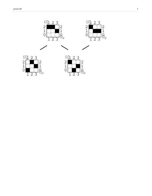
Figure 2: The posets for $\Omega_{1}=\{1,2\}$, $\Omega_{2}=\{1,2,3\}$.

We call a poset connected iff its cover graph is connected.

Lemma 4..7

The poset (4.4) is connected if and only if $n_{1}<n_{2}$.

Given $\pi\in{\mathcal{S}}$ we consider the convex and relatively open set

$${\mathcal{M}}_{\pi}(\Omega_{1},\Omega_{2}) := \Bigg{\{}p\in\overline{\mathcal{P}}(\Omega_{1}\times\Omega_{2})\;:\;\mbox{for all $\omega_{1}\in\Omega_{1}$,}$$

$$\sum_{\omega_{2}\in\pi^{-1}(\omega_{1})}p(\omega_{1},\omega_{2})=\frac{1}{n_{1}}\quad\mbox{and}\quad p(\omega_{1},\omega_{2})>0\ \mbox{iff}\ \pi(\omega_{2})=\omega_{1}\Bigg{\}}.$$

We denote by $S_{m,n}$ the Stirling numbers of the second kind (see for example [Ai]).

Theorem 4..8

(1) The set of global maximizers of the mutual information is a disjoint union

$${\mathcal{M}}(\Omega_{1},\Omega_{2})\;=\;{\biguplus}_{\pi\in{\mathcal{S}}}{\mathcal{M}}_{\pi}(\Omega_{1},\Omega_{2})$$

of sets ${\mathcal{M}}_{\pi}(\Omega_{1},\Omega_{2})$.
(2) These sets have dimension

$$\dim{\mathcal{M}}_{\pi}(\Omega_{1},\Omega_{2})\;=\;|\pi^{-1}(\Omega_{1})|-|\Omega_{1}|,$$

and there are $n_{1}!{n_{2}\choose l}S_{l,n_{1}}$ sets ${\mathcal{M}}_{\pi}(\Omega_{1},\Omega_{2})$ of dimension $l-n_{1}$.
(3) The inclusion ${\mathcal{M}}_{\sigma}(\Omega_{1},\Omega_{2})\subset\overline{{\mathcal{M}}_{\pi}}(\Omega_{1},\Omega_{2})$ holds if and only if $\sigma\preceq\pi$, and the set ${\mathcal{M}}(\Omega_{1},\Omega_{2})$ is connected if and only if $n_{1}<n_{2}$.

Example 4..9

Continuing Example 4..6, for $n_{1}=2$ and $n_{2}=3$ the set ${\mathcal{M}}(2,3)$ is the disjoint union of six points and six open intervals (see Figure 3, left), combined in the form of a hexagon (see Figure 3, right). So ${\mathcal{M}}(2,3)$ is homeomorphic to $S^{1}$ in this case.

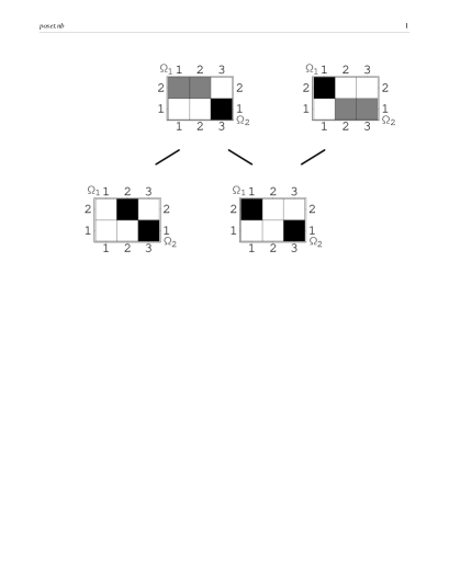
Figure 3: The structure of ${\mathcal{M}}(2,3)$.

4.3. The Case of $\boldsymbol{N}$ Equal Units

This section deals with the important example of $N$ units with $n_{1}=\dots=n_{N}=:n$. In that situation, Theorem 4..3 has the following direct implication.

Corollary 4..10

The set ${\mathcal{M}}(\Omega_{1},\dots,\Omega_{N})$ consists of all probability distributions

$$\frac{1}{n}\sum_{\omega_{N}\in\Omega_{N}}\delta_{(\pi_{1}(\omega_{N}),\dots,\pi_{N-1}(\omega_{N}),\omega_{N})},$$

where $\pi_{i}:\Omega_{N}\to\Omega_{i}$, $i=1,\dots,N-1$, are one-to-one mappings. This implies

$$|{\mathcal{M}}(\Omega_{1},\dots,\Omega_{N})|\;=\;(n!)^{N-1},$$ (4.5)

and for all $p\in{\mathcal{M}}(\Omega_{1},\dots,\Omega_{N})$,

$$I_{p}(X_{1},\dots,X_{N})\;=\;(N-1)\cdot\ln(n),$$

$$|{\rm supp}\,p|\;=\;n.$$ (4.6)

Thus according to (4.5), the number of the maximizers of the multi-information grows exponentially in $N$. In particular, for binary units the set ${\mathcal{M}}(\Omega_{1},\dots,\Omega_{N})$ has $2^{N-1}$ elements. In view of this fact, it is interesting that according to Corollary 3..1 there is an exponential family of dimension $\leq 3N+2$ that approximates all these global maximizers of the multi-information. This bound can even be improved. Although it is not our main goal to do that we close this subsection by an interesting $N$-independent upper bound, which implies that for $N$ binary units there exists an exponential family with dimension less than or equal to $5$ that approximates all $2^{N-1}$ elements of ${\mathcal{M}}(\Omega_{1},\dots,\Omega_{N})$.

Theorem 4..11

There exists an exponential family with dimension less than or equal to $(n^{2}+3n)/2$ that contains ${\mathcal{M}}(\Omega_{1},\dots,\Omega_{N})$ in its closure.

This exponential family, however, is based on multibody interactions (in terms of statistical mechanics) between the units $i\in[N]$.

5. Sufficiency of Low-Order Interaction for the Maximization of Multi-Information

Given a subset $A\subseteq[N]=\{1,\ldots,N\}$, we decompose $\omega\in\Omega_{V}$ in the form $\omega\;=\;(\omega_{A},\omega_{[N]\setminus A})$ with $\omega_{A}\in\Omega_{A}$, $\omega_{[N]\setminus A}\in\Omega_{[N]\setminus A}$. We define ${\mathcal{I}}_{A}$ to be the subspace of functions that do not depend on the configurations $\omega_{[N]\setminus A}$:

$${\mathcal{I}}_{A} := \left\{f\in{\mathbb{R}}^{\Omega_{V}}\;:\;\right.$$

$$\left.\mbox{$f(\omega_{A},\omega_{V\setminus A})=f(\omega_{A},\omega_{[N]\setminus A}^{\prime})$ for all $\omega_{A}\in\Omega_{A}$, and all $\omega_{[N]\setminus A},\omega_{[N]\setminus A}^{\prime}\in\Omega_{[N]\setminus A}$}\right\}.$$

The orthogonal projection $\Pi_{A}$ onto this $|\Omega_{A}|$-dimensional space with respect to the canonical scalar product

$$\langle f,g\rangle\;:=\;\sum_{\omega\in\Omega_{V}}f(\omega)g(\omega)\qquad(f,g\in{\mathbb{R}}^{\Omega_{V}})$$

in ${\mathbb{R}}^{\Omega_{V}}$ is given by

$$\Pi_{A}(f)(\omega_{A},\omega_{[N]\setminus A})\;:=\;\frac{1}{|\Omega_{[N]\setminus A}|}\sum_{\omega_{[N]\setminus A}^{\prime}\in\Omega_{[N]\setminus A}}f(\omega_{A},\omega_{[N]\setminus A}^{\prime}).$$

In order to describe only the pure contributions of $A$ to a function $f$, we ”subtract” the contributions from subsets $B\subsetneq A$. This leads to the $\prod_{i\in A}\big{(}|\Omega_{i}|-1\big{)}$-dimensional subspace

$$\widetilde{{\mathcal{I}}}_{A}\;:=\;{{\mathcal{I}}}_{A}\cap\left(\bigcap_{B\subsetneq A}{{\mathcal{I}}_{B}}^{\perp}\right)$$

and the orthogonal decomposition ${\mathbb{R}}^{\Omega_{V}}=\bigoplus_{A\subseteq[N]}\widetilde{{\mathcal{I}}}_{A}$. Denoting the orthogonal projections onto $\widetilde{{\mathcal{I}}}_{A}$ by $\widetilde{\Pi}_{A}$ we thus have $\widetilde{\Pi}_{A}\widetilde{\Pi}_{B}=\delta_{A,B}\widetilde{\Pi}_{A}$ and

$${\Pi}_{A}\;=\;\sum_{B\subseteq A}\widetilde{\Pi}_{B},\qquad A\subseteq[N],$$ (5.1)

and every vector $f$ has a unique representation as a sum of orthogonal vectors:

$$f\;=\;\sum_{A\subseteq[N]}\widetilde{\Pi}_{A}(f).$$

The $f_{A}$ is called (pure) interaction among the units in $A$. With the Möbius inversion (5.1) implies

$$\widetilde{\Pi}_{A}(f) = \sum_{B\subseteq A}(-1)^{|A\setminus B|}\Pi_{B}(f)$$

$$= \sum_{B\subseteq A}(-1)^{|A\setminus B|}\frac{1}{|\Omega_{[N]\setminus B}|}\sum_{\omega_{[N]\setminus B}^{\prime}\in\Omega_{[N]\setminus B}}f(\omega_{B},\omega_{[N]\setminus B}^{\prime}).$$

Now we construct exponential families associated with such interaction spaces. The most general construction is based on a set of subsets of $[N]$. Given such a set $\boldsymbol{A}\subseteq 2^{[N]}$, we define the corresponding interaction space by

$$\widetilde{{\mathcal{I}}}_{\boldsymbol{A}}\;:=\;\bigoplus_{A\in\boldsymbol{A}}\widetilde{{\mathcal{I}}}_{A},$$ (5.2)

which generates the exponential family $\exp(\widetilde{{\mathcal{I}}}_{\boldsymbol{A}})$. We want to apply this definition to the more specific situation of interactions with fixed order $k$. Therefore, we define

$${{\mathcal{I}}}^{(k)}\;:=\;\widetilde{{\mathcal{I}}}_{\{A\subseteq[N]\;:\;|A|\leq k\}},\qquad\mbox{and}\qquad\widetilde{{\mathcal{I}}}^{(k)}\;:=\;\widetilde{{\mathcal{I}}}_{\{A\subseteq[N]\;:\;|A|=k\}}.$$

We get the flag of vector spaces

$${\mathbb{R}}\cong{{\mathcal{I}}}^{(0)}\;\subsetneq\;{{\mathcal{I}}}^{(1)}\;\subsetneq\;{{\mathcal{I}}}^{(2)}\;\cdots\;\subsetneq{{\mathcal{I}}}^{(N)}={\mathbb{R}}^{\Omega_{V}},$$

and the corresponding hierarchy of exponential families

$$\exp({{\mathcal{I}}}^{(0)})\;\subsetneq\;\exp({{\mathcal{I}}}^{(1)})\;\subsetneq\;\exp({{\mathcal{I}}}^{(2)})\;\cdots\;\subsetneq\exp({{\mathcal{I}}}^{(N)})={\mathcal{P}}({\Omega_{V}}),$$

Here, $\exp({{\mathcal{I}}}^{(0)})$ contains exactly one element, namely the center of the simplex.

The exponential family $\exp({{\mathcal{I}}}^{(1)})$ is nothing but the exponential family ${\mathcal{F}}$ of factorizable distributions. Thus, the multi-information vanishes exactly on the topological closure of $\exp({{\mathcal{I}}}^{(1)})$.

Now we determine for a nonempty set ${\mathcal{M}}(\Omega_{1},\dots,\Omega_{N})$ of maximizers the lowest order $k$ such that ${\mathcal{M}}(\Omega_{1},\dots,\Omega_{N})$ is contained in the topological closure of $\exp({{\mathcal{I}}}^{(k)})$. The first possible candidate for this is given by $k=2$. The following theorem states that this is also sufficient.

Theorem 5..1

There exists an exponential family ${\mathcal{F}}^{*}\subseteq\exp(\widetilde{{\mathcal{I}}}^{(2)})$ of dimension $\dim({\mathcal{F}}^{*})=(n_{N}-1)\sum_{i=1}^{N-1}(n_{i}-1)$ containing in its closure all global maximizers of the multi-information (${\mathcal{M}}(\Omega_{1},\dots,\Omega_{N})\subset\overline{{\mathcal{F}}^{*}}$).

This theorem represents our main result which we already stated informally in Section 3. Note that compared with Theorem 4..11 for large $N$ Theorem 5..1 leads to an exponential family ${\mathcal{F}}^{*}$ of higher dimension. On the other hand, we still have an exponential (in $N$) codimension in the simplex $\overline{{\mathcal{P}}}(\Omega_{V})$.

In addition to that, the exponential family of Theorem 5..1 represents a concrete model that appears in many applications in physics and biology. For instance, within the field of neural networks, the exponential family $\exp({{\mathcal{I}}}^{(2)})$, which contains $\exp(\widetilde{{\mathcal{I}}}^{(2)})$ as a subfamily, is known as the family of Boltzmann machines, [AHS, AK, AKN]. Applied to this context, our result states that Boltzmann machines are able to generate all distributions that have globally maximal multi-information, and that their dimensionality ${N\choose 2}$ is not minimal for $N>2$.

Examples 5..2

(1) The Case of Two Units. In this case, the hierarchy of interactions ends with $k=2$, because we have just two units. Thus the simplex ${\mathcal{P}}(\Omega_{1}\times\Omega_{2})$ is equal to the exponential family $\exp({\mathcal{I}}^{(2)})$, which has dimension $n_{1}n_{2}-1$. The codimension of the subfamily $\exp(\widetilde{\mathcal{I}}^{(2)})$ of Theorem 5..1 then is $n_{1}+n_{2}-2$. Applied to our example of two binary units from the introduction, we see that

$$\dim(\exp(\widetilde{\mathcal{I}}^{(2)}))\;=\;1$$

In Figure 1, we obtain this family by simply taking the convex combinations of the two maximizers:

$$\exp(\widetilde{\mathcal{I}}^{(2)})\;=\;\left\{\frac{1-\lambda}{2}\left(\delta_{(0,0)}+\delta_{(1,1)}\right)+\frac{\lambda}{2}\left(\delta_{(1,0)}+\delta_{(0,1)}\right)\;:\;0<\lambda<1\right\}.$$

(2) The Case of $N$ Equal Units. According to Theorem 4..3 for $|\Omega_{i}|=n$ we have $|{\mathcal{M}}(\Omega_{1},\dots,\Omega_{N})|=(n!)^{N-1}$ maximizers, which are, according to Theorem 5..1, contained in the closure of an exponential family ${\mathcal{F}}^{*}$ of pure pair interactions, with

$$\dim({\mathcal{F}}^{*})=(N-1)(n-1)^{2}.$$

6. Proofs

We fix the following notations: For $V^{\prime}\subset[N]$, $H_{V^{\prime}}$ denotes the entropy of the random variable $X_{V^{\prime}}$. Obviously $H_{V}=H$, and $H_{\{i\}}=H_{i}$. For two subsets $V^{\prime},V^{\prime\prime}\subset[N]$, $H_{(V^{\prime\prime}\,|\,V^{\prime})}$ is the conditional entropy of $X_{V^{\prime\prime}}$ given $X_{V^{\prime}}$. For $V^{\prime}=\{a_{1},\dots,a_{L}\}$ and $V^{\prime\prime}=\{b_{1},\dots,b_{M}\}$ we also write $H_{(b_{1},\dots,b_{M}\,|\,a_{1},\dots,a_{L})}$ instead of $H_{(V^{\prime\prime}\,|\,V^{\prime})}=H_{(\{b_{1},\dots,b_{M}\}\,|\,\{a_{1},\dots,a_{L}\})}$. Now let $V_{1},\ldots,V_{r}$ be a set of disjoint subsets of $[N]=\{1,\ldots,N\}$. The multi-information of these subsystems is given by $I_{\{V_{1},\ldots,V_{r}\}}=\sum_{j=1}^{r}H_{V_{j}}-H_{V_{1}\uplus\dots\uplus V_{r}}$. In the case where the subsets of $[N]$ have cardinality one, we also write $I_{\{i_{1},\dots,i_{r}\}}$ instead of $I_{\{\{i_{1}\},\dots,\{i_{r}\}\}}$. We obviously have $I_{V}=I$.

Proof of Lemma 4..1.
By the chain rule $H(X,Y)=H(X)+H(Y\mid X)$

$$I_{p}(X_{1},\dots,X_{N})\;=\;\sum_{i=1}^{N}H_{p}(X_{i})\;-\;H_{p}(X_{1},\dots,X_{N})$$

$$= \sum_{i=1}^{N-1}H_{p}(X_{i})-\big{(}H_{p}(X_{1},\dots,X_{N})-H_{p}(X_{N})\big{)}$$

$$= \sum_{i=1}^{N-1}H_{p}(X_{i})-H_{p}(X_{1},\dots,X_{N-1}\mid X_{N})\leq\;\sum_{i=1}^{N-1}H_{p}(X_{i})\leq\sum_{i=1}^{N-1}\ln(n_{i}),$$

proving the lemma. $\Box$

Proof of Theorem 4..3.
If a probability distribution $p$ on $\Omega_{V}$ has the form (4.3) with a distribution $p^{(N)}\in\overline{\mathcal{P}}(\Omega_{N})$ and surjective maps $\pi_{i}:\Omega_{N}\rightarrow\Omega_{i}$ that satisfy (4.2), then $I(p)=\sum_{i=1}^{N-1}\ln(n_{i})$:

$$I(p)=\sum_{i=1}^{N}H_{i}(p)-H(p)$$

$$= \sum_{i=1}^{N}H_{i}(p)-H_{N}(p)\underbrace{-H_{(1|N)}(p)-H_{(2|1,N)}(p)-\dots-H_{(N-1|1,2,\dots,N-2,N)}(p)}_{=0}$$

$$= \sum_{i=1}^{N-1}\ln(n_{i}).$$

Now we prove the opposite implication. Therefore we assume $I(p)=\sum_{i=1}^{N-1}\ln(n_{i})$. This gives us

$$H_{i}(p)\;=\;\ln(n_{i})\qquad(i=1,\dots,N-1).$$ (6.1)

Otherwise the existence of an $i_{0}\in\{1,\dots,N-1\}$ with $H_{i_{0}}(p)<\ln(n_{i_{0}})$ would imply the following contradiction

$$I(p) = \sum_{i=1}^{N}H_{i}(p)-H(p)$$

$$= \sum_{i=1}^{N-1}H_{i}(p)+H_{N}(p)-\big{(}H_{N}(p)+H_{(1,\dots,N-1\,|\,N)}(p)\big{)}$$

$$\leq \sum_{i=1\atop i\not=i_{0}}^{N-1}H_{i}(p)+H_{i_{0}}(p)\;<\;\sum_{i=1}^{N-1}\ln(n_{i}).$$

From (6.1) we have

$$H(p)\;=\;\sum_{i=1}^{N}H_{i}(p)-I(p)\;=\;\left(\sum_{i=1}^{N-1}\ln(n_{i})+H_{N}(p)\right)-\sum_{i=1}^{N-1}\ln(n_{i})\;=\;H_{N}(p).$$ (6.2)

Now we set $p^{(N)}:=p_{N}$, and define a Markov kernel $K:(\Omega_{1}\times\cdots\times\Omega_{N-1})\times\Omega_{N}\rightarrow[0,1]$ by

$$K(\omega_{1},\dots,\omega_{N-1}\,|\,\omega_{N})\;:=\;\left\{\begin{array}[]{c@{,\quad}l}\frac{p(\omega_{1},\dots,\omega_{N})}{p_{N}(\omega_{N})}&\mbox{if $p_{N}(\omega_{N})>0$}\\ \frac{1}{n_{1}\cdots n_{N-1}}&\mbox{if $p_{N}(\omega_{N})=0$}\end{array}\right..$$

In these definitions we get

$$H(p)-H_{N}(p)$$

$$= \sum_{\omega_{N}\in\Omega_{N}\atop p_{N}(\omega_{N})>0}p_{N}(\omega_{N})\Bigg{(}\ln p_{N}(\omega_{N})-$$

$$\sum_{(\omega_{1},\dots,\omega_{N-1})\in\atop\Omega_{1}\times\cdots\times\Omega_{N-1}}K(\omega_{1},\dots,\omega_{N-1}\,|\,\omega_{N})\ln\Big{(}p_{N}(\omega_{N})\,K(\omega_{1},\dots,\omega_{N-1}\,|\,\omega_{N})\Big{)}\Bigg{)}$$

$$= \sum_{\omega_{N}\in\Omega_{N}\atop p_{N}(\omega_{N})>0}p_{N}(\omega_{N})\,H\big{(}K(\cdot\,|\,\omega_{N})\big{)}\;\geq\;0.$$

From (6.2) this implies $H\big{(}K(\cdot\,|\,\omega_{N})\big{)}=0$ for all $\omega_{N}$ with $p_{N}(\omega_{N})>0$. This implies the existence of maps $\pi_{i}:\Omega_{N}\rightarrow\Omega_{i}$ with

$$p(\omega_{1},\dots,\omega_{N})\;=\;p^{(N)}(\omega_{N})\prod_{i=1}^{N-1}\delta_{\omega_{i},\pi_{i}(\omega_{N})}.$$

Because of $H_{i}(p)=\ln(n_{i})$ for all $i\in\{1,\dots,N-1\}$, these maps must be surjective. $\Box$

Proof of Theorem 4..4.
Proof that ${\mathcal{M}}(\Omega_{1},\ldots,\Omega_{N})\neq\emptyset$ if $n_{N}\geq n_{\min}$:
For $m\in{\mathbb{N}}$ set $T_{m}:=\left\{\frac{i}{m}\ :\ i\in[m]\right\}$. We claim that the cardinality of

$$T_{\Omega}:=\bigcup_{i\in[N-1]}T_{n_{i}}$$

is given by $|T_{\Omega}|=n_{\min}$. This follows by the inclusion–exclusion principle if

$$\left|\bigcap_{i\in A}T_{n_{i}}\right|={\rm GCD}(n_{A})\qquad(A\in W),$$ (6.3)

since

$$\left|\bigcup_{i\in[N-1]}T_{n_{i}}\right|=\sum_{A\in W}(-1)^{|A|-1}\left|\bigcap_{i\in A}T_{n_{i}}\right|.$$

To prove (6.3), we set $m_{A}:={\rm GCD}(n_{A})$ and note that $T_{n_{i}}\supseteq T_{m_{A}}\ \ (i\in A)$. Thus $\left|\bigcap_{i\in A}T_{n_{i}}\right|\geq\left|T_{m_{A}}\right|=m_{A}$.

To show the converse inequality $\left|\bigcap_{i\in A}T_{n_{i}}\right|\leq m_{A}$ we note that for some $\tilde{m}\in{\mathbb{N}}$ we have $\bigcap_{i\in A}T_{n_{i}}=T_{\tilde{m}}$. Thus for all $i\in A$ there exist $\ell_{i}\in[n_{i}]$ with $\frac{\ell_{i}}{n_{i}}=\frac{1}{\tilde{m}}=\min(T_{\tilde{m}})$, or $n_{i}=\ell_{i}\tilde{m}$. Thus $\tilde{m}$ divides all $n_{i}\ \ (i\in A)$ and – being the largest such integer – equals $m_{A}={\rm GCD}(n_{A})$.

Now we write $T_{\Omega_{V}}$ in the form $\{d_{1},\ldots,d_{n_{\min}}\}$ and set $d_{0}:=0$, with ordering $d_{i}>d_{i-1}\ \ (i\in[n_{\min}])$. The map

$$\Phi:T_{\Omega_{V}}\to\Omega_{V}\quad\mbox{,}\quad\Phi(d_{j})_{i}:=\left\{\begin{array}[]{ccc}\lceil d_{j}n_{i}\rceil&,&i\in[N-1]\\ j&,&i=N\end{array}\right.$$

is well defined, since $\lceil d_{j}n_{i}\rceil\in[n_{i}]\ \ (i\in[N-1])$, and by our assumption $n_{N}\geq n_{\min}$ which implies $j\in[n_{N}]$. The function

$$p:\Omega_{V}\to{\mathbb{R}}\quad\mbox{,}\quad p:=\sum_{j=1}^{n_{\min}}(d_{j}-d_{j-1})\delta_{\Phi(d_{j})}$$ (6.4)

is a probability distribution since $d_{j}-d_{j-1}>0$ and

$$\sum_{j=1}^{n_{\min}}(d_{j}-d_{j-1})=d_{n_{\min}}-d_{0}=1.$$

For all $i\in[N-1]$ and $\ell\in[n_{i}]$ the $i$th marginal probability equals

$$p_{i}(\ell) = \sum_{\omega\in\times_{j\in[N]\backslash\{i\}}\ n_{j}}p(\ell,\omega)=\sum_{\stackrel{{\scriptstyle\omega_{N}\in[n_{\min}]}}{{\lceil d_{\omega_{N}}n_{i}\rceil=\ell}}}(d_{\omega_{N}}-d_{\omega_{N}-1})=$$

$$= \sum_{j:d_{j}\in\left(\frac{\ell-1}{n_{i}},\frac{\ell}{n_{i}}\right]}(d_{j}-d_{j-1})=\frac{\ell}{n_{i}}-\frac{\ell-1}{n_{i}}=\frac{1}{n_{i}}.$$

We thus meet the condition of Theorem 3.2 showing that $p\in{\mathcal{M}}(\Omega_{1},\ldots,\Omega_{N})$.

Proof that ${\mathcal{M}}(\Omega_{1},\ldots,\Omega_{N})=\emptyset$ if $n_{N}<n_{\min}$:

• The statement is trivial for $N=2$ (remember that we assume $n_{i+1}\geq n_{i}$). Assume now that it is proven for all product spaces of at most $N\in{\mathbb{N}}$ units. Then for a probability distribution $p\in{\mathcal{M}}(\Omega_{1},\ldots,\Omega_{N+1})$ consider its marginal ${\tilde{p}}\in\overline{{\mathcal{P}}}(\Omega_{[N]})$.
  We associate to ${\tilde{p}}$ a $N$–partite graph $(\tilde{V},E)$ whose vertex set is the disjoint union $\tilde{V}:=\dot{\bigcup}_{i=1}^{N}\Omega_{i}$. To every $\omega=(\omega_{1},\ldots,\omega_{N})\in{\rm supp}({\tilde{p}})\subseteq\Omega_{[N]}$ belongs the complete graph on the vertex set $\{\omega_{1},\ldots,\omega_{N}\}\subset\tilde{V}$ with edge set $G_{\omega}:=\big{\{}\{\omega_{i},\omega_{j}\}\subset\tilde{V}\mid 1\leq i<j\leq N\big{\}}$ on the $N$ vertices $\omega_{1},\ldots,\omega_{N}$. Then the edge set

  $$E:=\bigcup_{\omega\in{\rm supp}({\tilde{p}})}G_{\omega}$$

  on $\tilde{V}$ is indeed $N$–partite. By the strict positivity (4.2) of the $p$–marginals no vertex $v\in\tilde{V}$ is isolated.

• Every edge set $G_{\omega}\subseteq E$ is contained in the induced subgraph of exactly one connected component $C\subseteq\tilde{V}$ of the graph $(\tilde{V},E)$. We attribute to $G_{\omega}$ the weight ${\tilde{p}}(\omega)$, and to a connected component $C$ of the graph $(\tilde{V},E)$ the sum of the weights of the $G_{\omega}$ contained in it.

  Figure 4: A bipartite graph $(\tilde{V},G)$ for $N+1=3$ units, with $|\Omega_{1}|=4$, $|\Omega_{1}|=6$, $|\Omega_{3}|\geq 8$ and a maximizer $p\in{\mathcal{M}}(\Omega_{1},\Omega_{2},\Omega_{3})$. $(\tilde{V},G)$ has the two components $C_{1},C_{2}$.

  These weights $w(C)$ of the connected components $C$ are not arbitrary numbers in $(0,1]$. Instead, we know from Theorem 4..3 that the marginal distributions $p_{i}:\Omega_{i}\to[0,1]$ of $p$ (and thus of ${\tilde{p}}$, too) have the Laplace form

  $$p_{i}(\omega_{i})=\frac{1}{n_{i}}\qquad(i\in[N],\ \omega_{i}\in\Omega_{i}).$$

  Therefore $w(C)$ is simultaneously an integer multiple of $1/n_{i}\ \ (i\in[N])$ and thus an integer multiple of ${\rm GCD}(n_{[N]})$. This implies the upper bound ${\rm GCD}(n_{[N]})$ for the number of connected components $C$ of the $N$–partite graph $(\tilde{V},E)$.

• For the case of $N+1=3$ units this already suffices to show the bound $n_{3}\geq n_{\min}=n_{1}+n_{2}-{\rm GCD}(n_{1},n_{2})$. In this case the complete graphs are of cardinality $|G_{\omega}|=(N-1)!=1$ so that $|E|=|{\rm supp}({\tilde{p}})|$.
  In general a graph on a vertex set of $v\in{\mathbb{N}}$ vertices with $e\in{\mathbb{N}}_{0}$ edges has at least $\max(v-e,1)$ connected components. In the case at hand $v=n_{1}+n_{2}$, and there are at most ${\rm GCD}(n_{1},n_{2})$ connected components. So

  $$n_{3} \geq |{\rm supp}({p})|\geq|{\rm supp}(\tilde{p})|=|E|=e$$

  $$\geq v-c=(n_{1}+n_{2})-{\rm GCD}(n_{1},n_{2})=n_{\min}.$$

• For arbitrary $N+1>3$ this argument must be modified, since then $|G_{\omega}|=(N-1)!>1$.
  First of all we can substitute $G_{\omega}$ by any spannning tree $T_{\omega}\subset G_{\omega}$, and still the connected components $C^{\prime}$ of $(\tilde{V},E^{\prime})$ with $E^{\prime}:=\bigcup_{\omega\in{\rm supp}({\tilde{p}})}T_{\omega}$ coincide with the connected components $C$ of $(\tilde{V},E)$. Each of these spanning trees has only $|T_{\omega}|=N-1$ edges. However in general $E^{\prime}$, too is not a disjoint union of the $T_{\omega}$.
  We thus decompose the set ${\rm supp}({\tilde{p}})$ into a disjoint union

  $${\rm supp}({\tilde{p}})=\bigcup_{k=1}^{N}A_{k},$$ (6.5)

  beginning with an arbitrarily chosen set $A_{N}$ of representatives $\omega\in C$ of the connected components $C\subseteq\Omega_{[N]}$. The estimate on the number of these components implies $|A_{N}|\geq{\rm GCD}(n_{[N]})$, and for $\omega\neq\omega^{\prime}\in A_{N}$ the edge sets $G_{\omega}$ and $G_{\omega^{\prime}}$ are disjoint.
  Next we arrange the elements $\omega^{\prime}\in C$ of the connected component $C$ containing $\omega\in A_{N}$ in the form of a spanning tree, with $G_{\omega^{\prime}}\cap G_{\omega^{\prime\prime}}\neq\emptyset$ for $\{\omega^{\prime},\omega^{\prime\prime}\}$ being an edge of that tree. For $\omega^{\prime}=(\omega_{1}^{\prime},\ldots,\omega_{N}^{\prime})\in C$ of distance $d(\omega^{\prime})$ from $\omega\in A_{N}$ we put $\omega^{\prime}\in A_{k}$ if there are exactly $k$ indices $i\in[N]$ with $\omega_{i}^{\prime}$ not being equal to any $\omega_{i}^{\prime\prime}$ for $\omega^{\prime\prime}=(\omega_{1}^{\prime\prime},\ldots,\omega_{N}^{\prime\prime})$ with $d(\omega^{\prime\prime})<d(\omega^{\prime})$. This indeed gives a partition of the form (6.5).
  Then by our induction hypothesis

  $$|A_{k}|\geq\sum_{\stackrel{{\scriptstyle B\subseteq[N]}}{{|B|\geq k}}}(-1)^{|B|-k}{|B|\choose k}{\rm GCD}(n_{B})\qquad(k=1,\ldots,N).$$ (6.6)

  Namely for $k=N$ (6.6) reduces to $|A_{N}|\geq{\rm GCD}(n_{[N]})$ which has been shown to be true. So if (6.6) would not hold, for the smallest $k<N$ violating (6.6), we would find a $B\subseteq[N]$ of cardinality $|B|=k<N$, whose marginal distribution $p_{B}$ has support of cardinality $\hat{n}_{k+1}:=|{\rm supp}(p_{B})|<n_{\min}(B)=\sum_{\stackrel{{\scriptstyle\tilde{B}\subseteq B}}{{\tilde{B}\neq\emptyset}}}(-1)^{|\tilde{B}|-1}{\rm GCD}(n_{\tilde{B}})$, see (6.7) below.

  But this would contradict our induction assumption, since then the system $\hat{\Omega}:=\big{(}\times_{i\in B}[n_{i}]\big{)}\times[\hat{n}_{k+1}]$ would have the optimizing probability distribution

  $$\hat{p}:\hat{\Omega}\rightarrow[0,1]\quad\mbox{,}\quad\hat{p}(\omega_{B},l):=\delta_{e(l),\omega_{B}}\ p_{B}(\omega_{B})$$

  for some bijection $e:[\hat{n}_{k+1}]\rightarrow{\rm supp}(p_{B})$, but yet not meet the criterium $\hat{n}_{k+1}\geq n_{\min}(B)$.
  Summing the cardinalities (6.6), we obtain

  $$|{\rm supp}({\tilde{p}})| = \sum_{k=1}^{N}|A_{k}|\geq\sum_{k=1}^{[N]}\sum_{\stackrel{{\scriptstyle B\subseteq[N]}}{{|B|\geq k}}}(-1)^{|B|-k}{|B|\choose k}{\rm GCD}(n_{B})$$ (6.7)

  $$= \sum_{\stackrel{{\scriptstyle B\subseteq[N]}}{{B\neq\emptyset}}}(-1)^{|B|}{\rm GCD}(n_{B})\sum_{k=1}^{|B|}(-1)^{k}{|B|\choose k}$$

  $$= \sum_{\stackrel{{\scriptstyle B\subseteq[N]}}{{B\neq\emptyset}}}(-1)^{|B|-1}{\rm GCD}(n_{B})=n_{\min},$$

  which is the induction step. $\Box$

Proof of Lemma 4..7.
If $n_{1}=n_{2}$ then the maps $\pi\in{\mathcal{S}}$ are isomorphisms $\pi:\Omega_{2}\to\Omega_{1}$, so that $\sigma\preceq\pi$ only for $\sigma=\pi$. Thus in that case ${\mathcal{S}}$ is connected iff $|{\mathcal{S}}|=1$, i.e. $n_{1}=n_{2}=1$. This contradicts our assumption $n_{1},n_{2}\geq 2$.

If $n_{2}>n_{1}$ and $|\pi^{-1}(\omega_{1})|>1$ for $\pi\in{\mathcal{S}}$ and some $\omega_{1}\in\Omega_{1}$, say $\pi(\omega^{\prime}_{2})=\omega_{1}$, then $\sigma\preceq\pi$ for

$$\sigma\in{\mathcal{S}},\qquad\sigma(\omega_{2}):=\left\{\begin{array}[]{c@{,\quad}l}\pi(\omega_{2})&\mbox{if $\omega_{2}\neq\omega^{\prime}_{2}$}\\ 0&\mbox{if $\omega_{2}=\omega^{\prime}_{2}$}\end{array}\right..$$

So we need only show that any $\pi^{\prime},\pi^{\prime\prime}\in S$ which are injective onto $\Omega_{1}$ are indeed connected.

1. In the first step we move $\pi^{\prime}$ along the poset graph in order to decrease the cardinality of the symmetric difference $(\pi^{\prime})^{-1}(0)\Delta(\pi^{\prime\prime})^{-1}(0)$. So we assume that there exist

   $$\omega^{\prime}\in(\pi^{\prime})^{-1}(0)\backslash(\pi^{\prime\prime})^{-1}(0)\quad\mbox{and}\quad\omega^{\prime\prime}\in(\pi^{\prime\prime})^{-1}(0)\backslash(\pi^{\prime})^{-1}(0)$$

   and set

   $$\pi\in{\mathcal{S}},\qquad\pi(\omega):=\left\{\begin{array}[]{c@{,\quad}l}0&\mbox{if $\omega=\omega^{\prime\prime}$}\\ \pi^{\prime}(\omega^{\prime\prime})&\mbox{if $\omega=\omega^{\prime}$}\\ \pi^{\prime}(\omega)&\mbox{otherwise}.\end{array}\right.$$

   Both $\pi^{\prime}$ and $\pi$ are covered by

   $$\rho\in{\mathcal{S}},\qquad\rho(\omega):=\left\{\begin{array}[]{c@{,\quad}l}\pi^{\prime}(\omega^{\prime\prime})&\mbox{if $\omega=\omega^{\prime}$}\\ \pi^{\prime}(\omega)&\mbox{otherwise,}\end{array}\right.$$

   and

   $$|\pi^{-1}(0)\Delta(\pi^{\prime\prime})^{-1}(0)|\;=\;|(\pi^{\prime})^{-1}(0)\Delta(\pi^{\prime\prime})^{-1}(0)|-2.$$

   By iterating the argument we can assume w.l.o.g. that $(\pi^{\prime})^{-1}(0)=(\pi^{\prime\prime})^{-1}(0)$.

2. In fact it is sufficient to treat the case where the permutation

   $$\pi^{\prime\prime}\circ(\pi^{\prime})^{-1}\mid_{\Omega_{1}}:\Omega_{1}\to\Omega_{1}$$

   is a transposition, as the transpositions generate the symmetric group. So there exist $\omega^{I}\neq\omega^{II}\in\Omega_{2}$ with

   $$\pi^{\prime\prime}(\omega)=\left\{\begin{array}[]{c@{,\quad}l}\pi^{\prime}(\omega^{I})&\mbox{if $\omega=\omega^{II}$}\\ \pi^{\prime}(\omega^{II})&\mbox{if $\omega=\omega^{I}$}\\ \pi^{\prime}(\omega)&\mbox{otherwise,}\end{array}\right.$$

   and we choose $\hat{\omega}\in\Omega_{2}$ so that $\pi^{\prime}(\hat{\omega})=\pi^{\prime\prime}(\hat{\omega})=0$.

   Defining $\rho,\rho^{\prime\prime}\in{\mathcal{S}}$ by

   $$\rho^{\prime}(\omega):=\left\{\begin{array}[]{c@{,\quad}l}\pi^{\prime}(\omega^{II})&\mbox{if $\omega=\hat{\omega}$}\\ 0&\mbox{if $\omega=\omega^{II}$}\\ \pi^{\prime}(\omega)&\mbox{otherwise}\end{array}\right.\quad\mbox{resp.}\quad\rho^{\prime\prime}(\omega):=\left\{\begin{array}[]{c@{,\quad}l}\pi^{\prime\prime}(\omega^{I})&\mbox{if $\omega=\hat{\omega}$}\\ 0&\mbox{if $\omega=\omega^{I}$}\\ \pi^{\prime\prime}(\omega)&\mbox{otherwise,}\end{array}\right.$$

   $\pi^{\prime}$ and $\rho^{\prime}$ are covered by $\sigma^{\prime}\in{\mathcal{S}}$ and similarly $\pi^{\prime\prime}$ and $\rho^{\prime\prime}$ are covered by $\sigma^{\prime\prime}\in{\mathcal{S}}$ with

   $$\sigma^{\prime\prime}(\omega):=\left\{\begin{array}[]{c@{,\quad}l}\pi^{\prime}(\omega^{II})&\mbox{if $\omega=\hat{\omega}$}\\ \pi^{\prime}(\omega)&\mbox{otherwise}\end{array}\right.\quad\mbox{resp.}\quad\sigma^{\prime\prime}(\omega):=\left\{\begin{array}[]{c@{,\quad}l}\pi^{\prime\prime}(\omega^{I})&\mbox{if $\omega=\hat{\omega}$}\\ \pi^{\prime\prime}(\omega)&\mbox{otherwise.}\end{array}\right.$$

   Now as $\pi^{\prime}(\omega^{II})=\pi^{\prime\prime}(\omega^{I})$, both $\rho^{\prime}$ and $\rho^{\prime\prime}$ are covered by

   $$\tau\in{\mathcal{S}},\qquad\tau(\omega):=\left\{\begin{array}[]{c@{,\quad}l}\pi^{\prime}(\omega^{II})&\mbox{if $\omega=\hat{\omega}$}\\ \pi^{\prime}(\omega^{I})&\mbox{if $\omega=\omega^{II}$}\\ \pi^{\prime}(\omega)&\mbox{otherwise.}\end{array}\right.$$

   This shows that the poset graph is connected. $\Box$

Proof of Theorem 4..8.
To simplify notation, we set ${\mathcal{M}}:={\mathcal{M}}(\Omega_{1},\Omega_{2})$, and ${\mathcal{M}}_{\pi}:={\mathcal{M}}_{\pi}(\Omega_{1},\Omega_{2})$ for $\pi\in{\mathcal{S}}$.
(1) We have ${\mathcal{M}}_{\pi}\subset{\mathcal{M}}$ since for the elements of ${\mathcal{M}}_{\pi}$ the characterisation of Theorem 4..3 hold true. Furthermore for $\sigma,\pi\in{\mathcal{S}}$ with $\sigma\neq\pi$ there exists $(\omega_{2},\omega_{1})\in{\rm graph}(\pi)$ with $(\omega_{2},\omega_{1})\not\in{\rm graph}(\sigma)$ or vice versa. Thus for $p\in{\mathcal{M}}_{\pi}$ we have $p(\omega_{1},\omega_{2})>0$ but for $p\in{\mathcal{M}}_{\sigma}$ we have $p(\omega_{1},\omega_{2})=0$ showing that ${\mathcal{M}}_{\pi}\cap{\mathcal{M}}_{\sigma}=\emptyset$.
Finally for $p\in{\mathcal{M}}$ by Theorem 4..3 there exists a surjective map $\tilde{\pi}:\Omega_{2}\to\Omega_{1}$ with $p(\omega_{1},\omega_{2})=0$ whenever $\tilde{\pi}(\omega_{2})\neq\omega_{1}$. Given $\tilde{\pi}$, we construct $\pi\in{\mathcal{S}}$ by setting

$$\pi(\omega_{2}):=\left\{\begin{array}[]{c@{,\quad}l}\tilde{\pi}(\omega_{2})&\mbox{if $p(\tilde{\pi}(\omega_{2}),\omega_{2})>0$}\\ 0&\mbox{if $p(\tilde{\pi}(\omega_{2}),\omega_{2})=0$}.\end{array}\right.$$

As by Theorem 4..3 we have $\sum_{\omega_{2}\in\tilde{\pi}^{-1}(\omega_{1})}p(\omega_{1},\omega_{2})=\frac{1}{n_{1}}>0$, the function $\pi:\Omega_{2}\to\Omega_{1}^{*}$ so constructed has the property $\pi(\Omega_{2})\supset\Omega_{1}$ making it an element of $S$.
(2) Given $\omega_{1}\in\Omega_{1}$, the simplex of $|\pi^{-1}(\omega_{1})|$ numbers $p(\omega_{1},\omega_{2})>0$ with $\omega_{2}\in\pi^{-1}(\omega_{1})$ meeting $\sum_{\omega_{2}\in\pi^{-1}(\omega_{1})}p(\omega_{1},\omega_{2})=\frac{1}{n_{1}}$ has dimension $|\pi^{-1}(\omega_{1})|-1$, implying the formula for $\dim{\mathcal{M}}_{\pi}$.
If $\dim{\mathcal{M}}_{\pi}=l-n_{1}$, the surjective map $\hat{\pi}:\hat{\Omega}_{2}\to\Omega_{1}$ with $\hat{\Omega}_{2}:=\pi^{-1}(\Omega_{1})\subset\Omega_{2}$ and $\hat{\pi}:=\pi\mid_{\hat{\Omega}_{2}}$ is defined on a subset $\hat{\Omega}_{2}\subset\Omega_{2}$ of size $l$. There are precisely ${n_{2}\choose l}$ such subsets, and there are precisely $n_{1}!S_{l,n_{1}}$ such surjective maps from $\hat{\Omega}_{2}$ onto $\Omega_{1}$, see Aigner [Ai], Chapter 3.1.
(3) If $n_{1}=n_{2}$ then ${\mathcal{S}}$ coincides with the set of bijections $\pi:\Omega_{2}\to\Omega_{1}$, and $|{\mathcal{M}}_{\pi}|=1$. Thus in this case ${\mathcal{M}}$ is not connected for $n_{1}\geq 2$. If, however $n_{2}>n_{1}$, the poset ${\mathcal{S}}$, seen as a graph, is connected.
The topological closure of ${\mathcal{M}}_{\pi}$ is given by

$$\overline{{\mathcal{M}}}_{\pi}=\left\{p\in\overline{\mathcal{P}}(\Omega_{1}\times\Omega_{2})\;:\;\sum_{\omega_{2}\in\pi^{-1}(\omega_{1})}p(\omega_{1},\omega_{2})=\frac{1}{n_{1}},p(\omega_{1},\omega_{2})=0\ \mbox{if}\ \pi(\omega_{2})\neq\omega_{1}\right\}.$$

Thus $\overline{{\mathcal{M}}}_{\pi}={\biguplus}_{\sigma\preceq\pi}{\mathcal{M}}_{\sigma}$. $\Box$

Proof of Corollary 4..10.
All statements directly follow from Theorem 4..3 . $\Box$

Proof of Theorem 4..11.
We choose a map $\phi=(\phi_{1},\dots,\phi_{n}):\;\Omega_{V}\;\rightarrow\;{\mathbb{R}}^{n}$ such that the points $\phi(\omega)$, $\omega\in\Omega_{V}$, are in general position; that is, each $k$ elements of $\phi(\Omega_{V})$ with $k\leq n+1$ are affinely independent. This property guarantees that for each set $\Sigma\subset\Omega_{V}$, $|\Sigma|=n$, there exist real numbers $a_{1},\dots,a_{n},b$ such that

$$\left\{\omega\in\Omega_{V}\;:\;\sum_{i=1}^{n}a_{i}\,\phi_{i}(\omega)=b\right\}\;=\;\Sigma$$ (6.8)

holds. We consider the exponential family ${\mathcal{G}}^{\ast}$ that is generated by $c$ and

$$\phi_{1},\dots,\phi_{n}\quad\mbox{,}\quad\phi_{i}\,\phi_{j}\quad(1\leq i\leq j\leq n).$$

We have

$$\dim{\mathcal{G}}^{\ast}\;\leq\;\frac{n^{2}+3n}{2}.$$

Now let $p$ be an element of ${\mathcal{M}}(N\times n)$. From Theorem 4..10 we know that $|{\rm supp}\,p|\;=\;n$. We prove that there exists a sequence in ${\mathcal{G}}^{\ast}$ that converges to $p$. We choose a sequence $\beta_{m}\uparrow\infty$ and real numbers $a_{1},\dots,a_{n},b$ satisfying (6.8) with $\Sigma={\rm supp}\,p$. Then with

$$E^{(m)}\;:=\;-\beta_{m}\left(\sum_{i=1}^{n}a_{i}\,\phi_{i}\;-\;b\right)^{2},$$

the sequence

$$\frac{\exp E^{(m)}}{\sum_{\omega^{\prime}\in\Omega_{V}}\exp E^{(m)}(\omega^{\prime})}\;\in\;{\mathcal{G}}^{\ast}$$

converges to $p$. $\Box$
Proof of Theorem 5..1.
Using def. (5.2), we consider for $\boldsymbol{A}:=\{\{1,N\},\{2,N\},\ldots,\{N-1,N\}\}\subset 2^{[N]}$ the linear subspace

$$\widetilde{{\mathcal{I}}}_{\boldsymbol{A}}\subset\widehat{{\mathcal{I}}}_{2}$$

of pure pair interactions of the $N$th unit with all other units. The exponential family ${\mathcal{F}}^{*}:=\exp(\widetilde{{\mathcal{I}}}_{\boldsymbol{A}})\subset{\mathcal{P}}(\Omega_{V})$ is of dimension

$$\dim({\mathcal{F}}^{*})=(n_{N}-1)\sum_{i=1}^{N-1}(n_{i}-1),$$

as asserted in Theorem 5..1.

Given a maximizer $p\in{\mathcal{M}}(\Omega_{1},\ldots,\Omega_{N})$, we now construct a sequence of probability distributions

$$q^{(m)}:=\exp(\tilde{f}^{(m)})\in{\mathcal{F}}^{*}\qquad(m\in{\mathbb{N}})$$

and show that $\lim_{m\rightarrow\infty}q^{(m)}=p$.

Here the functions $\tilde{f}^{(m)}\in\widetilde{{\mathcal{I}}}_{\boldsymbol{A}}$ are defined as the orthogonal projections onto $\widetilde{{\mathcal{I}}}_{\boldsymbol{A}}$ of ${f}^{(m)}\in{{\mathcal{I}}}^{(2)}$

$${f}^{(m)}(\omega):=\prod_{i=1}^{N-1}\delta_{\omega_{i},\pi_{i}(\omega_{N})}\ \frac{m+\ln\left(p^{(N)}(\omega_{N})+1/m\right)}{N-1}\qquad(\omega\in\Omega_{V}).$$

For $\omega,\omega^{\prime}\in{\rm supp}(p)$

$$\frac{q^{(m)}(\omega)}{q^{(m)}(\omega^{\prime})} = \exp\left(\left[m+\ln\left(p^{(N)}(\omega_{N})+\frac{1}{m}\right)\right]\!\!-\!\!\left[m+\ln\left(p^{(N)}(\omega_{N}^{\prime})+\frac{1}{m}\right)\right]\right)$$

$$= \frac{p^{(N)}(\omega_{N})+\frac{1}{m}}{p^{(N)}(\omega_{N}^{\prime})+\frac{1}{m}}\ \stackrel{{\scriptstyle m\rightarrow\infty}}{{\longrightarrow}}\ \frac{p^{(N)}(\omega_{N})}{p^{(N)}(\omega_{N}^{\prime})}$$

in accordance with (4.3).

On the other hand if $\omega^{\prime}\in{\rm supp}(p)$ but $\omega\not\in{\rm supp}(p)$, then there is an $i\in\{1,\ldots,N-1\}$ with $\omega_{N}\neq\pi_{i}^{-1}(\omega_{i})$ or $p^{(N)}(\omega_{N})=0$. In both cases

$$\lim_{m\to\infty}\frac{q^{(m)}(\omega)}{q^{(m)}(\omega^{\prime})}=0,$$

again in accordance with (4.3). As the $p^{(m)}$ are probability distributions, we have shown that $\lim_{m\rightarrow\infty}q^{(m)}=p$. $\Box$

Nihat Ay

Max Planck Institute for Mathematics in the Sciences,

Inselstr. 22, D 04103 Leipzig, nay@mis.mpg.de

Andreas Knauf

Mathematisches Institut, Friedrich-Alexander-Universität Erlangen-Nürnberg, Bismarckstr. 1 1/2, D-91054 Erlangen, Germany, knauf@mi.uni-erlangen.de