Exact and quasi-resonances in discrete water-wave turbulence

Abstract

The structure of discrete resonances in water-wave turbulence is studied. It is shown that the number of exact 4-wave resonances is huge (hundreds million) even in comparatively small spectral domain when both scale and angle energy transport is taken into account. It is also shown that angle transport can contribute inexplicitly to scale transport. Restrictions for quasi-resonances to start are written out. The general approach can be applied directly to mesoscopic systems encountered in condensed matter (quantum dots), medical physics, etc.

Pacs: 47.35.Bb, 89.75.Kd

1. Introduction. Statistical wave turbulence theory deals with the fields of dispersively interacting waves. Examples of these wave systems can be found in oceans, atmospheres, plasma, etc. Interactions between waves are similar to interactions between particles and can be described by kinetic equations (KEs) analogous to KE known in quantum mechanics since 1930th. Wave KE is in fact one limiting case of the quantum Bose-Einstein equation while the Boltzman kinetic equation is its other limit. First wave KE for surface gravity waves has been presented in has while general method of construction KEs for many other types of waves can be found in lvov . One of the major achievements of the statistical approach is establishing of the fact that power energy spectra (similar to famous Kolmogorov 5/3 law) are exact stationary solutions of kinetic equations zak2 . The limitations of statistical turbulence theory are due to the fact that it does not describe spatial unevenness of turbulence, i.e. organized structures extending over many scales, like boulders in a waterfall, remain unexplained. Appearance of these structures is attributed to mesoscopic regimes which are at the frontier between classical (single waves/particles) and statistical (infinite number of waves/particles) description of physical systems. Mesoscopic (effectively zero-dimensioned) systems is very popular topic in various areas of modern physics - from wave turbulence to condensed matter (quantum dots, dots ) to medical physics. For instance, in med1 dynamics of blood flow in humans is studied, cardiovascular system is described by a few coupled oscillators and synchronization conditions are investigated. Synchronization or resonance conditions have the same general form for wave and quantum systems (see, for instance, spohn for 4-photon processes); and have to be studied in integers. Just for simplicity of presentation we prefer to stay with wave terminology while all examples in this Letter are taken from wave turbulent systems.

Resonance conditions have the form

$$\omega_{1}\pm\omega_{2}\pm...\pm\omega_{s}=0,\quad\vec{k}_{1}\pm\vec{k}_{2}\pm....\pm\vec{k}_{s}=0$$ (1)

where $\ \omega_{i}=\omega(\vec{k}_{i}),\ \ s<\infty,\$ with $\ \vec{k}\$ and $\omega_{i}=\omega(\vec{k}_{i})$ being correspondingly wave vector and dispersion function. Specific features of these systems described by Fourier harmonics with integer mode numbers were first presented in PRL (we call them further discrete wave systems, DWS). A counter part to kinetic equation in DWS is a set of few independent dynamical systems of ODEs on the amplitudes of interacting waves. Mathematical theory of DWS was developed in AMS with general understanding that discrete effects are only important in some bounded part of spectral space, $\ |\vec{k}|<k_{0},\$ with some small finite $\ k_{0}\$, while the case $\ |\vec{k}|>>k_{0}\$ is covered by kinetic equations and power-law energy spectra. This general opinion was broken recently as result of numerical simulations with Euler equations for capillary waves zak3 and for surface gravity waves zak4 where discrete clusters of waves were observed simultaneously with statistical regime. Moreover, experimental results DLN06 show that discrete effects are major and statistical wave turbulence predictions are never achieved: with increasing wave intensity the nonlinearity becomes strong before the system loses sensitivity to the $\ \vec{k}$-space discreteness.

2. Discrete wave systems. In lam a model is presented which explains the appearance of discrete wave clusters in the large spectral domains with $\ |\vec{k}|>>k_{0}.\$ It shows that energy power spectra are valid not in all spectral domain with big $\ \vec{k}\$ but have ”holes” all over the spectrum, in some integer $\ \vec{k},\$ which describe discrete dynamics of mesoscopic regimes. This understanding put ahead a novel computational problem - computing integer solutions of (1) in the large spectral domains. Indeed, (1) turns into

$$\sqrt{k_{1}}+\sqrt{k_{2}}=\sqrt{k_{3}}+\sqrt{k_{4}},\quad\vec{k}_{1}+\vec{k}_{2}=\vec{k}_{3}+\vec{k}_{4},$$ (2)

for 4-wave interactions of 2D-gravity water waves, where $\vec{k}_{i}=(m_{i},n_{i}),\ \forall i=1,2,3,4$ and $k_{i}=|\vec{k}_{i}|=\sqrt{m_{i}^{2}+n_{i}^{2}}$. This means that in a domain, say $\ |m|,|n|\leq D\sim 1000\$, direct approach leads to necessity to perform extensive (computational complexity $\ D^{8}$) computations with integers of the order of $10^{12}$. The full search for multivariate problems in integers consumes exponentially more time with each variable and size of the domain to be explored. The use of special form of resonance conditions allowed us to develop fast generic algorithms comp_all for solving systems of the form (1) in integers. The main idea of the algorithms for irrational dispersion function is that if vectors $\ \vec{k}_{i}\$ construct an integer solution of (1), then at least for some $i_{0},j_{0}$ the ratios $\omega_{i_{0}}/\omega_{j_{0}}$ have to be rational numbers. Some other number-theoretical considerations were used in case of rational dispersion functions. In particular, all integer solutions of (2) in domain $\ |m|,|n|\leq 1000\$ were found in a few minutes at a Pentium-3 (cf.: direct search for them in smaller domain $\ |m|,|n|\leq 128$ took 3 days with Pentium-4 naz1 ).

Using our programs we studied how the structure of discrete resonances depends on the form of dispersion function and on the chosen $s$. The interesting fact is that characteristic structure is the same for different dispersion functions (examples with $\omega=m/n(n+1),\ \omega=1/\sqrt{m^{2}+n^{2}},\ \omega=m/(n^{2}+m^{2}+1)$ and others were studied) if $s=3$. Most waves do not take part in resonances and interacting waves form small independent clusters, with no energy flow between clusters due to exact resonances. Our conclusion about wave systems with 3-wave interactions is therefore that exact resonances are rare and quasi-resonances, i.e. those satisfying

$$\omega_{1}\pm\omega_{2}\pm...\pm\omega_{s}=\Omega>0,\quad\vec{k}_{1}\pm\vec{k}_{2}\pm....\pm\vec{k}_{s}=0$$ (3)

with $\ s=3\$ can be of importance for some applications. The situation changes substantially in the case $\ s\geq 4\$ which is illustrated below with surface gravity waves taken as our main example.

3. Exact resonances. The major difference between 3- and 4-wave interactions can be briefly formulated as follows. Any 3-wave resonance generates new wave lengths and therefore takes part in energy transfer over scales. In a system with 4-wave resonances two mechanisms of energy transport are possible: 1) over scales, if at least one new wave length is generated, and 2) over angles, if no new wave lengths are generated. Examples of these two types of solutions for (2) are $(-80,-76)(980,931)\ \Rightarrow\ (180,171)(720,684)$ and $(-1,4)(2,-5)\ \Rightarrow\ (-4,1)(5,-2)$, we call these solutions further scale- and angle-resonances correspondingly. Two mechanisms of energy transport provide substantially richer structure of resonances and the number of exact resonances grows enormously when compared to 3-wave resonance system. Say, for dispersion $\omega=1/\sqrt{m^{2}+n^{2}}$ and 3-wave interactions there exist only 28156 exact resonances with $|m|,|n|\leq 1000$ while for dispersion $\omega=(m^{2}+n^{2})^{1/4}$ and 4-wave interactions in the same domain the overall number of exact resonances is about 600 million. However, major part of these resonances are angle-resonances. In the domain $\ |m|,|n|\leq 1000\$ we have found only 3945 scale-resonances, i.e. transport over the scales is similar to the case of 3-wave interactions. Some isolated quartets do exist, also among angle-resonances, for instance $(-1,-1)(1,1)\ \Rightarrow\ (-1,1)(1,-1)$ but they are rather rare. Very important fact is that angle and scale energy transport are not independent in following sense. One wave, say (64,0), takes part in 2 scale-resonances one of them being $(64,0)(135,180)\ \Rightarrow\ (80,60)(119,120)$ and the wave (119,120) takes part then in 12 angle-resonances, and further on (see Figs.1,2).

It is important to understand that for $\ s>4\$ 1) no new type of resonances appear, and 2) existence of angle-resonances depends on the placing of signs in the first equation of (1): for instance, if it has the form $\omega_{1}=\omega_{2}+...+\omega_{s},$ no angle-resonances are possible.

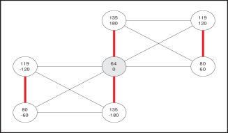
Figure 1: Wave (64,0) takes part in 2 scale-resonances. The upper number in the circle is $m$ and the lower - $n$, and red thick lines drawn between vectors on the same side of the Eqs.(2).

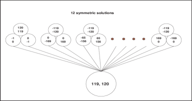
Figure 2: Wave (119,120) takes part in 12 angle-resonances.

The natural question now is whether quasi-resonances are in fact of importance in a wave system possessing such enormous number of exact resonances.

4. Quasi-resonances. From now on we are interested in discrete quasi-resonances which are integer solutions of (3) with some non-zero resonance width $\ \Omega.\$ Notice that $\ \omega:\mathbb{Z}\times\mathbb{Z}\rightarrow\mathbb{Q}(q)\$, where $\ q\$ is an algebraic number of degree 4 and the field $\ \mathbb{Q}(q)\$ denotes corresponding algebraic expansion of $\ \mathbb{Q}\$. To estimate a linear combination of different $\omega_{i}$ over $\ \mathbb{Q}\$ we use generalization of the Thue-Siegel-Roth theorem tue : If the algebraic numbers $\ \alpha_{1},\alpha_{2},...,\alpha_{s}\$ are linearly independent with 1 over $\ \mathbb{Q}\$, then for any $\ \varepsilon>0\$ we have $|p_{1}\alpha_{1}+p_{2}\alpha_{2}+...+p_{s}\alpha_{s}-p|>cp^{-s-\varepsilon}$ for all $\ p,p_{1},p_{2},...,p_{s}\in\mathbb{Z}\$ with $\ p=\max_{i}|p_{i}|.\$ The non-zero constant $\ c\$ has to be constructed for every specific set of algebraic numbers separately. For $\ \omega=(m^{2}+n^{2})^{1/4}\$ and four-term combination this statement means in particular that $\ |\omega_{1}\pm\omega_{2}\pm\omega_{3}\pm\omega_{4}|>1\$ if at least one of $\ \omega_{i}\$ is not a rational number. As it was pointed out in comp_all all integer solutions of (2) have one of two forms: I) $\ \omega_{i}=\gamma_{i}q^{1/4},\ \forall i=1,2,3,4\$ or II) $\ \omega_{1}=\omega_{3}=\gamma_{1}q_{1}^{1/4},\ \omega_{2}=\omega_{4}=\gamma_{2}q_{2}^{1/4},\ q_{1}\neq\ q_{2}.\$ Here $\ \gamma_{i},q,q_{1},q_{2}\$ are some integers and $\ q,q_{1},q_{2}\$ have form $\ p_{1}^{e_{1}}p_{2}^{e_{2}}...p_{n}^{e_{n}},\$ with all different primes $\ p_{1},...p_{n}\$ while the powers $\ e_{1},...e_{n}\in\hbox{\Sets N}\cup\{0\}\$ are integers all smaller than $4$. It follows that for all wave vectors but those of the form I) with $\ q=1,\$ there exists a global low boundary for resonance width, $\ \Omega>1,\$ necessary to start quasi-resonances. In the spectral domain $\ |m|,|n|\leq 1000\$ only 136 scale-resonances do not have global low boundary. But even for them local low boundary exists - defined by the spectral domain $\ T=\{(m,n):0<|m|,|n|\leq D<\infty\}\$ chosen for numerical simulations. Indeed, let us define $\ \Omega_{D}=\min_{p}\Omega_{p},\$ where $\Omega_{p}=|\omega(\vec{k}^{p}_{1})\pm\omega(\vec{k}^{p}_{2})\pm...\pm\omega(\vec{k}^{p}_{4})|,\ \ \vec{k}^{p}_{j}=(m^{p}_{j},n^{p}_{j})\in T,$ for $\forall j=1,2,3,4,$ $\ \omega(\vec{k}^{p}_{1})\pm\omega(\vec{k}^{p}_{2})\pm...\pm\omega(\vec{k}^{p}_{4})\neq 0\quad\forall p,\$ and index $\ p\$ runs over all wave vectors in $\ T\$, i.e. $\ p\leq 4D^{2}\$. So defined $\ \Omega_{p}\$ obviously is a non-zero number as a minimum of finite number of non-zero numbers and $\ \Omega_{D}\$ is minimal resonance width which allows discrete quasi-resonances to start, for chosen $\ D.$

Step of numerical schema $\ 0<\delta\ll 1\$ is another parameter important for understanding quasi-resonant regimes, and inter-relation between $\ \delta,\$ $\ \Omega_{D}\$ and $\ \Omega\$ describes them all. For instance, if $\ \Omega_{D}>\Omega,\$ any chosen $\ \delta_{0}>\Omega_{D}\$ will allow some number of quasi-resonances, say $\ N_{(\delta_{o}>\Omega_{D})}\$, and for any $\ \delta>\delta_{0}\ \ \Rightarrow\ \ N_{(\delta>\Omega_{D})}\geq N_{(\delta_{o}>\Omega_{D})}.\$ On the other side, if $\ \delta\$ is decreasing to $\ \Omega_{D}\$ from above, $\ \delta\rightarrow\Omega_{D}+0,\$ the number of quasi-resonances reaches some constant level $\ N_{min}\$, $\ N_{min}=N_{(\delta=\Omega_{D})}\$. If $\ \delta\$ is increasing to $\ \Omega_{D}\$ from below, $\ \delta\rightarrow\Omega_{D}-0,\$ the number of quasi-resonances is $\ N_{min}=\mathop{\rm const}\nolimits.\$

This fact has been first discovered in the numerical simulations Tan2004 , both for capillary and surface gravity waves (maximal spectral domain studied was $\ 0<m\leq 2047,\ 0<n\leq 1023\$ and only scale-resonances were regarded). In case of gravity surface waves, increasing of $\ \Omega\$ from $10^{-10}$ to $10^{-5}$ does not changes number $\ N\$ of quasi-resonances while increasing of $\ \Omega\$ from $\ 10^{-4}\$ to $\ 10^{-3}\$ yields increasing $\ N\rightarrow 10N.\$ It turned out that limiting level $\ N_{min}\$ is 0 for capillary and and $\ \sim 10^{5}\$ for surface waves, for the same discretization by a rectangular mesh. It was attributed to the following fact: quasi-resonances are formed in some vicinity of exact resonances which do exist in the case of gravity waves and are absent in the case of capillary waves.

5. Topological structure of resonances. Graphical presentation of discrete 2D-wave clusters suggested in AMS is to regard each 2D-vector as a node of integer lattice in spectral space and connect those nodes which construct one solution (triad, quartet, etc.) We demonstrate it in Fig.3 (upper panel) taking for simplicity 3-wave interactions with $\omega=1/\sqrt{m^{2}+n^{2}}$ (ocean planetary waves). Obviously, geometrical structure is too nebulous to be useful. On the other hand, topological structure in Fig.3 (lower panel) is quite clear and gives us immediate information about the form dynamical equations covering behavior of each cluster. The number in brackets shows how many times corresponding cluster appears in the chosen spectral domain. All similar clusters are covered by similar systems of ODEs (written for simplicity for real-valued amplitudes): $\ \dot{A}_{1}=\alpha_{1}A_{2}A_{3},\ \dot{A}_{2}=\alpha_{2}A_{1}A_{3},\ \dot{A}_{3}=\alpha_{3}A_{1}A_{2},\$ in the case of a ”triangle” group, two coupled systems of this form in the case of ”butterfly” group and so on.

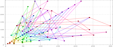
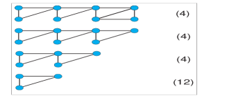
Figure 3: Upper panel: Geometrical structure, $D=300$. Lower panel: Topological structure, $D=50$. The number in brackets shows how many times corresponding cluster appears in the chosen spectral domain.

A 3-wave system has been chosen here as an illustrative example for its simplicity. They have only one type of vertices in their graphical presentations: nodes, corresponding to exact resonances. Some graph-theoretical considerations allow to construct isomorphism between topological elements of the solution set of (1) and corresponding dynamical systems, for the case $\ s=3.\$ This yields a constructive method to generate all different dynamical systems in a given spectral domain. For instance, all graphs shown in Fig.3, lower panel, are described by 4 different dynamical systems; for all isomorphic graphs, corresponding dynamical system has the same form though coupling coefficients $\ \alpha_{i}\$ have different magnitudes, of course. Some programs are written in MATHEMATICA which allow for a few specific examples to a) find all integer solutions of (1), b) generate their geometrical and topological structure, c) write out explicitly all corresponding dynamical systems. Only small number of these systems are known to be solvable analytically (mostly those corresponding to clusters of 3 to 5 waves only) while larger systems should be solved numerically, of course. Knowledge of specific form of a dynamical system allows in many cases to write out some conservation laws and thus simplify substantially further numerical simulations.

In case of $\ s$-wave interactions with $\ s\geq 4\$ construction of a corresponding graph must be substantially refined: a graph with 3 different types of vertices should be constructed, corresponding to the waves taking part in 1) angle-resonances, 2) scale-resonances, 3) both types of resonances, in order to provide simultaneous isomorphism of graphs and dynamical systems. This work is under the way.

Knowledge of the resonances structure might contribute to short-term forecast of wave field evolution, for in direct numerical simulations Tan2004 ,T07 discrete resonances were observable not at the time scale $O(t/\varepsilon^{4})$ of kinetic theory ($\varepsilon$ is steepness of wave field) but at linear time scale $t.$

6. Conclusions.

1. 3-wave systems can possess only scale-resonances which are rare, in this case quasi-resonances might be of importance in energy transport;

2. $s$-wave systems with $\ s\geq 4,\$ depending on the sign setting in (1), may also posses angle-resonances which contribute inexplicitly into energy transport. In systems like (2) where angle-resonances are allowed, there exist hundreds million of exact resonances in a comparatively small spectral domain $\ |m|,|n|\leq 1000.\$

3. For some polynomial irrational dispersion function, global low boundary $\ \Omega\$ for quasi-resonances to start can be computed which 1) does not depend on the chosen spectral domain, and 2) is valid for the most part of exact resonances in a system. If dispersion is a rational function, only local low boundary $\ \Omega_{D}\$ exists (it follows from the fact that   ℚ   is dense everywhere in   ℝ).

4. Any interpretation of results of numerical simulations with dispersive wave systems has to take into account interplay between $\ \delta,\$ $\ \Omega_{D}\$ and $\ \Omega.\$

5. Specially developed graph presentation of the solution set of (1) allows to construct isomorphism between independent cluster of resonantly interacting waves and corresponding dynamical systems. This yields constructive algorithm for generating dynamical systems symbolically, for instance using MATHEMATICA.

6. The same approach (the use of the algorithms from comp_all , low boundary computing, graph construction and generation of dynamical systems) can be used directly for any mesoscopic system with resonances of the form (1) or, more generally, of the form

$$p_{1}\omega_{1}\pm p_{2}\omega_{2}\pm...\pm p_{s}\omega_{s}=0,\quad p_{1}\vec{k}_{1}\pm p_{2}\vec{k}_{2}\pm....\pm p_{s}\vec{k}_{s}=0$$

with integer $\ p_{i},\$ in this case global low boundary will depend on $\ \max_{i}|p_{i}|$.

Acknowledgements. Author acknowledges the support of the Austrian Science Foundation (FWF) under projects SFB F013/F1304. Author expresses special gratitude to S. Nazarenko and M.Tanaka for stimulating discussions; to Ch. Feurer, G. Mayrhofer, C. Raab and O. Rudenko for MATHEMATICA programming, and to anonymous referees for valuable recommendations.

References

- (1) K. Hasselman. J. Fluid Mech. 12, 481 (1962)
- (2) V.E. Zakharov, V.S. L’vov, G. Falkovich. Kolmogorov Spectra of Turbulence. Series in Nonlinear Dynamics, Springer (1992)
- (3) V.E.Zakharov, N.N. Filonenko. J. Appl. Mech. Tech. Phys., 4, 500 (1967)
- (4) R.D. Schaller, V.I. Klimov. PRL 96, 097402 (2006)
- (5) A. Stefanovska, M.B. Lotric, S. Strle, H. Haken. Physiol. Meas. 22, 535; doi:10.1088/0967-3334/22/3/311 (2001)
- (6) H. Spohn. E-print arXiv:math-ph/0605069 (2006)
- (7) E.A. Kartashova. PRL , 72, 2013 (1994)
- (8) E.A. Kartashova. AMS Transl. 182 (2), 95 (1998)
- (9) A.N. Pushkarev, V.E. Zakharov. Physica D, 135, 98 (2000)
- (10) V.E. Zakharov, A.O. Korotkevich, A.N. Pushkarev, A.I. Dyachenko. JETP Letters, 82 (8), 491 (2005)
- (11) P. Denissenko, S. Lukaschuk, S. Nazarenko. E-print: arXiv.org:nlin.CD/0610015 (2006)
- (12) E.A. Kartashova. JETP Letters, 83 (7), 345 (2006)
- (13) E. Kartashova. JLTP 145 (1-4), 295 (2006); E. Kartashova, A. Kartashov: IJMPC 17 (11), 1579 (2006); CiCP 2 (4), 783 (2007); Physica A: Stat. Mech. Appl. to appear (2007)
- (14) S. Nazarenko. Personal communication (12.2005)
- (15) W.M. Schmidt. Diophantine approximations. Math. Lecture Notes 785, Springer, Berlin, 1980
- (16) M. Tanaka, N. Yokoyama. Fluid Dynamics Research 34, 216 (2004)
- (17) M. Tanaka. J. Fluid Mech. 444, 199 (2001); M. Tanaka. J. Phys. Oceanogr., to appear (2007)