New physical wavelet ’Gaussian Wave Packet’

Abstract

An exact solution of the homogeneous wave equation, which was found previously, is treated from the point of view of continuous wavelet analysis (CWA). If time is a fixed parameter, the solution represents a new multidimensional mother wavelet for the CWA. Both the wavelet and its Fourier transform are given by explicit formulas and are exponentially localized. The wavelet is directional. The widths of the wavelet and the uncertainty relation are investigated numerically. If a certain parameter is large, the wavelet behaves asymptotically as the Morlet wavelet. The solution is a new physical wavelet in the definition of Kaiser, it may be interpreted as a sum of two parts: an advanced and a retarded part, both being fields of a pulsed point source moving at a speed of wave propagation along a straight line in complex space-time.

Department of Mathematical Physics, Physics Faculty,
St.Petersburg University,
Ulyanovskaya 1-1, Petrodvorets, St.Petersburg, 198904, Russia
mailto: perel@mph.phys.spbu.ru, M.Sidorenko@ms8466.spb.edu

Keywords: physical wavelet, acoustic wavelet, localized wave, pulse, wave equation, mother wavelet, continuous wavelet analysis

1 Introduction

The wavelet analysis has a great many different applications in signal and image processing (see [1], [2]), in physics and astronomy (see [4], [5], [6]). It is also used for developing efficient numerical algorithms for solving differential equations [7], [8]; however, mother wavelets are usually not associated with the solutions of differential equations under consideration.

There is also an analytic approach to the problems of wave propagation proposed by Kaiser [9], where the technique of wavelet analysis is developed for the decomposition of solutions of the wave equation in terms of localized solutions, which are called physical wavelets. They are constructed by means of a special technique of analytic continuation of fundamental solutions in complex space-time and can be split into two parts: an advanced fundamental solution and a retarded one. The physical wavelet as a localized solution of the wave equation has also been given in [10]. Applications of physical wavelets were discussed in [11]-[16].

In the present paper, we treat a new wavelet, which is at the same time a localized solution of the homogeneous wave equation in two or more dimensions. This solution has been previously found and discussed in [17], [18] and generalized in [19]. It was named the Gaussian Wave Packet. We study its properties from two points of view. First, the solution can be taken as a mother wavelet for continuous wavelet analysis if time is a parameter and can be used in signal processing without being connected with any differential equation. Secondly, this solution should be regarded as a physical wavelet, i.e., it is an analytic continuation to the complex space-time of the sum of advanced and retarded parts of the field of a point source moving at a speed of wave propagation along a straight line and emitting a pulse that is localized in time. It is natural to decompose nonstationary wave fields in terms of these solutions, using the techniques of wavelet analysis.

The aim of the paper is a detailed investigation of wavelet properties of the Gaussian Wave Packet for a fixed time and its properties as a solution of the wave equation in view of its further application to problems of wave propagation. For example, the decomposition of the solution of the initial value problem for the wave equation in terms of wavelets has been proposed by us in [20].

In Section 2, we give a brief review of the main facts of continuous wavelet analysis in one and two dimensions.

In Section 3, we show that the Gaussian Wave Packet for a fixed time can be regarded as a wavelet, give some estimates of it, and present its Fourier transform. We show that both the wavelet and its Fourier transform have an exponential decay at infinity. The wavelet has not only zero mean but all zero moments as well.

In Section 4, we discuss the asymptotic behavior of the Gaussian Wave Packet as some of the free parameters become large. We compare the packet with the nonstationary Gaussian Beam [21], i.e., with the solution of the wave equation localized near the axis. We give the Gaussian asymptotic of it reducing it to the Morlet well-known wavelet [5].

In Section 5, we discuss the results of numerical calculations of the centers and widths of the packet in both the space and spatial frequency domains. We specify how fast these characteristics tend to asymptotic ones, with respect to the Morlet wavelet. We investigate the Heisenberg uncertainty relation for this wavelet, depending on the parameters and check how far from the saturation it is. We also obtain results for the nonasymptotic case where the wavelet corresponds to the solution that describes the propagation of the wave packet of one oscillation. This case may find applications in optics. We specify when the wavelet is directional [3] and calculate its scale and angular resolving powers.

Section 6 gives a generalization of the above results to the case of an arbitrary number of spatial dimensions.

In Section 7, we establish an analogy between the new wavelet and physical wavelets of Kaiser [9]. We show that it may split into incoming and outgoing parts, each solving a nonhomogeneous wave equation. As a source, we take new one-dimensional time-dependent wavelets, moving in the complex space-time at a speed of light.

2 Main formulas of continuous wavelet
analysis

Wavelet analysis is a method for analyzing local spectral properties of functions (for example, see [1] - [4]). Wavelet analysis also allows one to represent any function of finite energy as the superposition of a family of functions called wavelets derived from one function called a mother wavelet by shifting and scaling its argument in the one-dimensional case and also by rotating it in the case of several spatial dimensions. By analogy, the Fourier transform represents a signal as the superposition of oscillating exponents derived from one exponent by changing its frequency.

2.1 One-dimensional wavelet analysis

Let us give a brief review of some basic facts concerning the wavelet analysis of functions dependent on one variable $x$ (for more detail, see [1] - [4], [9]). Let a function $\varphi(x)$ have a zero mean, and let it decrease as $|x|$ tends to infinity so fast that $\varphi(x)\in\mathbb{L}_{1}(\mathbb{R})\bigcap\mathbb{L}_{2}(\mathbb{R})$. It must oscillate to be nonzero and to have the zero mean. We call such a function a ’mother wavelet’ because we derive a two-parametric family of functions from it, using two operations that shift the argument by $b$ and scale it by $a$:

$$\varphi^{a,b}(x)=\frac{1}{|a|^{1/2}}\,\varphi\left(\frac{x-b}{a}\right),\qquad b\in(-\infty,\infty),\,\,a\in(-\infty,+\infty).$$ (1)

Thus any function $\varphi^{a,b}(x)$ from this family again has the shape of $\varphi$, but shifted and dilated. By means of these operations, we can ’place’ $\varphi(x)$ at any point of the $x$ axis and change its ’size’ to any size by the parameter $a$. Then we define the wavelet transform $W(a,b)$ of any signal $f(x)$ by the formula

$$W(a,b)=\int\limits_{\mathbb{R}}\,dx^{\prime}\,f(x^{\prime})\,\overline{\varphi^{a,b}(x^{\prime})},$$ (2)

where the bar over $\varphi$ denotes complex conjugation.

One of the best-known mother wavelets is the Morlet wavelet, which is

$$\varphi(x)=\exp\left(-\frac{x^{2}}{2\sigma^{2}}\right)\left[\exp(-i\kappa x)-\exp(-\kappa^{2}\sigma^{2}/2)\right].$$ (3)

It is the difference of a Gaussian function, filled with oscillations, and a term that provides the zero mean of $\varphi(x)$ and that is negligible if $\kappa\sigma\gg 1.$ It is clear from formulas (1) - (3) that $|W(a,b)|^{2}$, defined by (2), provides information about the frequency content of the signal $f$ in the vicinity of the size $a\sigma$ of the point $b$, and $\kappa/a$ plays the role of a spatial frequency. So we may regard the wavelet transform as a window transform, the size of a window changing for different frequencies. Changing the size of the window makes the wavelet transform more precise as compared to the Window Fourier (or Gabor) transform.

We can also reconstruct the signal $f(x)$ from its wavelet transform $W(a,b)$, or, in other words, represent the signal $f(x)$ as a superposition of elementary signals $\varphi^{a,b}(x)$. Moreover, the mother wavelet used for the reconstruction of $f(x)$ may differ from the one used for the analysis. The reconstruction formula looks like this

$$f(x)=\frac{1}{C_{\varphi\psi}}\int\limits_{0}^{\infty}\,\frac{da}{a^{2}}\,\int\limits_{-\infty}^{\infty}\,db\,W(a,b)\,\psi^{a,b}(x),$$ (4)

where $\psi(x)$ is another mother wavelet, and the constant $C_{\varphi\psi}$ reads

$$C_{\varphi\psi}=\int\limits_{-\infty}^{\infty}\,dk\,\frac{\widehat{\varphi}(k)\overline{\widehat{\psi}(k)}}{|k|},$$ (5)

where the symbol $\widehat{}$ denotes the Fourier transform. If we use the same wavelet for the transform and reconstruction, we should put $\widehat{\psi}(k)=\widehat{\varphi}(k)$ and get $|\widehat{\varphi}(k)|^{2}$ in this formula to calculate the coefficient $C_{\varphi\varphi}\equiv C_{\varphi}.$

2.2 Wavelet analysis in two dimensions

Wavelet analysis can also be defined for the case of more than one dimension (see [5], [14], [15]). A mother wavelet in the case of two dimensions $\boldsymbol{r}=(x,y)$ is a function $\varphi(\boldsymbol{r})\in\mathbb{L}_{1}(\mathbb{R}^{2})\bigcap\mathbb{L}_{2}(\mathbb{R}^{2})$ that has zero mean. The Morlet wavelet in two dimensions reads

$$\varphi(\boldsymbol{r})=\exp\left(-\frac{x^{2}}{2\sigma_{\mathrm{x}}^{2}}-\frac{y^{2}}{2\sigma_{\mathrm{y}}^{2}}\right)\left[\exp(-i\kappa x)-\exp(-\kappa^{2}\sigma_{\mathrm{x}}^{2}/2)\right].$$ (6)

We define a family of wavelets from the mother wavelet, introducing rotations as well as dilations and the vector translations as follows:

$$\varphi^{a,\alpha,\boldsymbol{b}}(\boldsymbol{r})=\frac{1}{a}\varphi\left(\boldsymbol{M}_{\alpha}^{-1}\frac{\boldsymbol{r}-\boldsymbol{b}}{a}\right),\qquad\boldsymbol{M}_{\alpha}^{-1}=\left(\begin{array}[]{cc}\cos\alpha&-\sin\alpha\\ \sin\alpha&\cos\alpha\end{array}\right).$$ (7)

The wavelet transform is defined as

$$W(a,\alpha,\boldsymbol{b})=\int\limits_{\mathbb{R}^{2}}\,d^{2}\boldsymbol{r^{\prime}}\,f(\boldsymbol{r^{\prime}})\,\overline{\varphi^{a,\alpha,\boldsymbol{b}}(\boldsymbol{r^{\prime}})},\quad\boldsymbol{r^{\prime}}=(x^{\prime},y^{\prime}),\ \ d^{2}\boldsymbol{r^{\prime}}=dx^{\prime}\,dy^{\prime}.$$ (8)

Then the reconstruction formula takes the form

$$f(\boldsymbol{r})=\frac{1}{C_{\varphi\psi}}\int\limits_{0}^{\infty}\,\frac{da}{a^{3}}\,\int\limits_{\mathbb{R}^{2}}\,d^{2}\boldsymbol{b}\,\int\limits_{0}^{2\pi}\,d\alpha\,W(a,\alpha,\boldsymbol{b})\,\psi^{a,\alpha,\boldsymbol{b}}(\boldsymbol{r}),$$ (9)

where

$$C_{\varphi\psi}=\int\limits_{\mathbb{R}^{2}}\,d^{2}\boldsymbol{k}\,\frac{\widehat{\varphi}(\boldsymbol{k})\overline{\widehat{\psi}(\boldsymbol{k})}}{|\boldsymbol{k}|^{2}},\qquad\boldsymbol{k}=(k_{\mathrm{x}},k_{\mathrm{y}}),\qquad d^{2}\boldsymbol{k}=dk_{\mathrm{x}}\,dk_{\mathrm{y}},$$ (10)

and the Fourier transform $\widehat{\psi}(\boldsymbol{k})$ is

$$\widehat{\psi}(\boldsymbol{k})=\int\limits_{\mathbb{R}^{2}}d^{2}\boldsymbol{r}\,\psi(\boldsymbol{r})\,\exp{(-i\boldsymbol{k}\cdot\boldsymbol{r})},\qquad d^{2}\boldsymbol{r}=dx\,dy.$$ (11)

3 New two-dimensional wavelets

We consider a family of functions $\psi(\boldsymbol{r})$ of two spatial variables $x,y$ containing arbitrary real parameters $t,\nu$ and positive parameters $p$, $\varepsilon,$ $\gamma$ :

$$\psi(\boldsymbol{r})=\sqrt{\frac{2}{\pi}}\;\frac{(ps)^{\nu}\,K_{\nu}(ps)}{\sqrt{x+ct-i\varepsilon}},\qquad\boldsymbol{r}=(x,y),$$ (12)

$$s=\sqrt{1-i{\theta}/{\gamma}},\qquad\qquad$$ (13)

$$\theta=x-ct+\frac{y^{2}}{x+ct-i\varepsilon},$$ (14)

where $K_{\nu}$ is the Bessel modified function (MacDonald’s function) [23]. The branch of the square root in formula (13) with positive real part is taken. The choice of the branch of the square root in the denominator of (12) is not important, for the sake of definiteness we assume that it has positive real part. We intend to show that each of the functions from the family (12) is suited for the role of a mother wavelet with good properties. The same is valid for their derivatives of any order with respect to spatial coordinates and time.

Function (12) has appeared in [19] in connection with the linear wave equation

$$\psi_{tt}-c^{2}(\psi_{xx}+\psi_{yy})=0,\qquad c=const.$$ (15)

If we regard the parameter $t$ as time, formula (12) gives an exact solution of (15), which is well localized if $p\gg 1$ (see below). If $\nu={1\over 2},$ formula (12) yields

$$\psi(\boldsymbol{r})=\frac{\exp{(-ps)}}{\sqrt{x+ct-i\varepsilon}}.$$ (16)

If in addition $\varepsilon=\gamma,$ it leads to the exact solution of (15) which was first reported in [17] and discussed in detail in [18].

In this section we view $\psi$ as a two-dimensional mother wavelet with $t$ being a parameter, ignoring that it is a solution of (15). According to [1], [5], this is possible, provided that the following conditions are satisfied:

$$\int\limits_{\mathbb{R}^{2}}\,d^{2}\boldsymbol{r}\,|\psi(\boldsymbol{r})|<\infty,\qquad\int\limits_{\mathbb{R}^{2}}\,d^{2}\boldsymbol{r}\,|\psi(\boldsymbol{r})|^{2}<\infty,\qquad d^{2}\boldsymbol{r}\equiv dx\,dy,$$ (17)

i.e., $\psi(\boldsymbol{r})\in\mathbb{L}_{1}(\mathbb{R}^{2})\bigcap\mathbb{L}_{2}(\mathbb{R}^{2}),$ and it has zero mean, i.e.,

$$\int\limits_{\mathbb{R}^{2}}\,d^{2}\boldsymbol{r}\,\psi(\boldsymbol{r})=0.$$ (18)

To prove (17) we note that formulas (13), (14) imply that $\mathrm{Re}(s^{2})\geq 1$ and thus we get $\mathrm{Re}(s)\geq 1,$ $|\arg(s)|<\pi/4$. Therefore, (12) has neither singularities nor branch points for real $x,y$ and $t$. It is a smooth function of $x,y,t,$ and its derivatives of any order with respect to $x,y,t$ are also smooth functions. We also obtain

$$|s^{2}|^{2}=1+\frac{(x-ct)^{2}+y^{2}}{\gamma^{2}}+\frac{y^{2}((x-ct)^{2}+y^{2}+2\varepsilon\gamma-\varepsilon^{2}-4(ct)^{2})}{\gamma^{2}[(x+ct)^{2}+\varepsilon^{2}]}.$$ (19)

If $x$ and $y$ are large to an extent that the third term in (19) is positive, then

$$|s^{2}|^{2}>\frac{(x-ct)^{2}+y^{2}}{\gamma^{2}}.$$ (20)

Hence for large $x$ and $y$ the Bessel modified function can be replaced by its asymptotics, resulting in

$$\psi(\boldsymbol{r})\,=\,\frac{(ps)^{\nu-1/2}\,\exp{(-ps)}}{\sqrt{x+ct-i\varepsilon}}\;\left[1+O\left(\frac{1}{|ps|}\right)\right].$$ (21)

Noting that $\mathrm{Re}(s)\geq|s|/\sqrt{2}$ because $|\arg(s)|<\pi/4,$ we conclude that $\psi(\boldsymbol{r})$ has an exponential falloff and $\psi\in\mathbb{L}_{1}\bigcap\mathbb{L}_{2}.$

To check that the condition (18) is satisfied, we calculate the Fourier transform of $\psi(\boldsymbol{r})$

$$\widehat{\psi}(\boldsymbol{k})=\int\limits_{\mathbb{R}^{2}}d^{2}\boldsymbol{r}\,\psi(\boldsymbol{r})\,\exp{(-i\boldsymbol{k}\cdot\boldsymbol{r})},\qquad\boldsymbol{k}=(k_{\mathrm{x}},k_{\mathrm{y}}).$$ (22)

The calculations yield (see Appendix 1)

$$\widehat{\psi}(\boldsymbol{k})=2\pi\,e^{i\pi/4}\frac{p^{2\nu}}{\gamma^{\nu}}\,\left[k(k+k_{\mathrm{x}})^{\nu+1/2}\right]^{-1}\,$$

$$\times\exp\left[-(k+k_{\mathrm{x}})\frac{\gamma}{2}-(k-k_{\mathrm{x}})\frac{\varepsilon}{2}-\frac{p^{2}}{2\gamma(k+k_{\mathrm{x}})}-ikct\right],$$ (23)

where $k=|\boldsymbol{k}|$. The formula (23) shows that $\widehat{\psi}(\boldsymbol{k})|_{{k}=0}=0,$ owing the term in the exponent containing the denominator $k+k_{\mathrm{x}}$. Therefore, the function $\psi(\boldsymbol{r})$ has zero mean (18). Conditions (17), (18) enable $\psi(\boldsymbol{r})$ to be a mother wavelet.

Moreover, the following relation holds:

$$\left.\frac{\partial^{l+m}\left[k_{\mathrm{x}}^{j}\;k_{\mathrm{y}}^{\mu}\;\widehat{\psi}(\boldsymbol{k})\right]}{\partial^{l}k_{\mathrm{x}}\;\partial^{m}k_{\mathrm{y}}}\right|_{{k}=0}=0$$ (24)

for any integer nonnegative $j$, $\mu$, $l$, and $m$. This condition, the smoothness and the exponential falloff of $\psi(\boldsymbol{r})$ mean that any derivative of $\psi$ may be viewed as a mother wavelet and that all the moments of the wavelet $\psi$ and its derivatives vanish, i.e.,

$$\int\limits_{\mathbb{R}^{2}}d^{2}{\boldsymbol{r}}\,x^{l}y^{m}\,\psi(\boldsymbol{r})\,=\,0,\qquad\int\limits_{\mathbb{R}^{2}}d^{2}{\boldsymbol{r}}\,x^{l}y^{m}\,\frac{\partial^{j+\mu}\;\psi(\boldsymbol{r})}{\partial^{j}x\;\partial^{\mu}y}\,=\,0.$$ (25)

This property indicates that such wavelets could be useful in singular fields [1]-[5].

The wavelet $\psi$ has simple asymptotics for large values of $p$, which is discussed in the next section. Below we present calculations of the wavelet (12) and its Fourier transform (23) for moderate values of $p$ when no asymptotics can be applied. It should be mentioned that the wavelet (12) represents a wave of one oscillation when $\sqrt{p}\approx 1$ (see Figures 1, 2). This case is applicable in optics in the case of propagation of short pulses.

(a) Plot of the real part of $\psi(\boldsymbol{r}).$

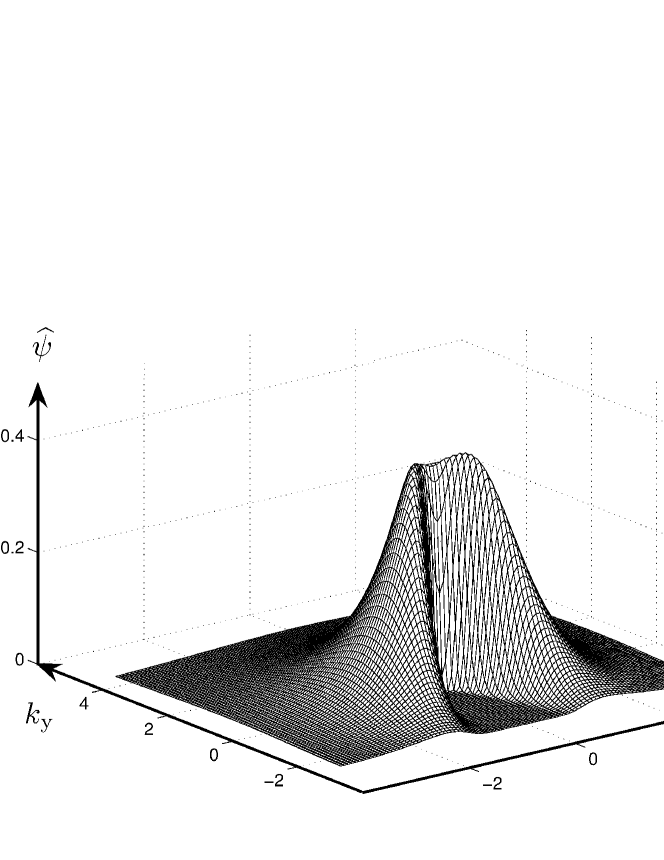
(b) Plot of the Fourier transform $\widehat{\psi}(\boldsymbol{k}).$

Figure 1: An example of the new wavelet and its Fourier transform for $p=0.5,\,\,\varepsilon=1,\,\,\gamma=0.25.$

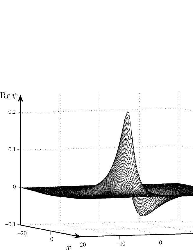
(a) Plot of the real part of $\psi(\boldsymbol{r}).$

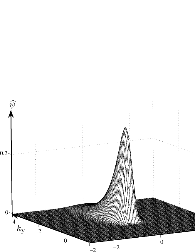
(b) Plot of the Fourier transform $\widehat{\psi}(\boldsymbol{k}).$

Figure 2: An example of the new wavelet and its Fourier transform for $p=1,\,\,\varepsilon=16,\,\,\gamma=0.5.$

4 Simple asymptotics of the wavelet

In this section, we study asymptotic properties of the Gaussian Wave Packet when the parameter $p$ is large. First we note that we can replace the McDonald function in (12) by its exponential asymptotics (see [23]) and then we get (21) for any $x,y,t$ if $p\gg 1$. To prove this, we show that $\mathrm{Re}(s)\geq 1$, then $\mathrm{Re}(ps)\geq p\gg 1$, which provides that $|ps|\gg 1$ and the exponential asymptotics is suitable.

We intend to show first that the modulus of the exponent in (21) has a maximum at the point $x=ct,y=0$. Let $s=a+ib,$ then the relation $2a^{2}=(a^{2}-b^{2})+(a^{2}+b^{2})$ yields

$$2[\mathrm{Re}(s)]^{2}=\mathrm{Re}(s^{2})+\sqrt{[\mathrm{Re}(s^{2})]^{2}+[\mathrm{Im}(s^{2})]^{2}}.$$ (26)

Hence $[\mathrm{Re}(s)]^{2}\geq\mathrm{Re}(s^{2})$, and taking into account that first

$$\mathrm{Re}(s^{2})=1+\frac{\varepsilon y^{2}}{\gamma\;[\;(x+ct)^{2}\;+\;\varepsilon^{2}\;]}$$ (27)

and secondly

$$|s^{2}|^{2}=1+\frac{(x-ct)^{2}}{\gamma^{2}},$$ (28)

which follows from (19) if $y=0$, we get $\mathrm{Re}(s)>1$ outside the point $x=ct,$ $y=0.$ Formulas (13), (14) show that $s=1$ if $x=ct,y=0,$ which is the point of the maximum of the modulus of exponent (21). Hence $\mathrm{Re}(s)\geq 1$, next $\mathrm{Re}(ps)\gg 1,$ and the asymptotics (21) can be used.

Now we study the behavior of the Gaussian Wave Packet near its maximum and show that it can be approximated by a nonstationary Gaussian beam. Consider a domain near the point $x=ct,y=0$ which is of order

$$\frac{x-ct}{\gamma}=O\left(\frac{1}{p^{\alpha}}\right),\quad\frac{y}{\sqrt{\varepsilon\gamma}}=O\left(\frac{1}{p^{\alpha}}\right),\qquad{1\over 3}\,<\,\alpha\,<\,{1\over 2}.$$ (29)

We prove below that the wavelet $\psi(\boldsymbol{r})$ has a uniform asymptotics in this domain as $p\to\infty$ :

$$\psi(\boldsymbol{r})=\psi_{\mathrm{beam}}(\kappa,\boldsymbol{r})\,\exp\left[-\frac{\kappa(x-ct)^{2}}{4\gamma}\right]C\left[1+O\left(p^{-3\alpha+1}\right)\right],$$ (30)

where $\kappa=p/(2\gamma)$ and $\psi_{\mathrm{beam}}$ is a nonstationary Gaussian beam [21], [22]

$$\psi_{\mathrm{beam}}(\kappa,\boldsymbol{r})=\frac{\exp{(i\,\kappa\,\theta)}}{\sqrt{x+ct-i\varepsilon}},$$ (31)

$$C=p^{\nu-1/2}\exp{(-p)}.$$ (32)

To prove (30), we decompose $s$ from (13) into powers of $\theta/\gamma$, which are of order $O(p^{-\alpha})$ by the formula (29) and the inequality $\left|{{y^{2}}/{(x+ct-i\varepsilon)}}\right|<{y^{2}/\varepsilon}$. We obtain

$$s=\sqrt{1-i{\theta}/{\gamma}}=1-i{{\theta}\over{2\gamma}}+{{\theta^{2}}\over{8\gamma^{2}}}+{\cal E}_{1}.$$ (33)

We insert (33) into (21), substituting the expression for $\theta$ (14) and the quadratic term ${{\theta^{2}}/{(8\gamma^{2})}}={{(x-ct)^{2}}/{(8\gamma^{2})}}+{\cal E}_{2}$ into it. It is easy to show that

$$\exp[-p({\cal E}_{1}+{\cal E}_{2})]=1+O\left(p^{-3\alpha+1}\right).$$ (34)

We also note that the multiplier $s^{\nu}$ of the McDonald function in formula (12) has an estimate $s^{\nu}=1+O(p^{-\alpha})$ and $O(p^{-\alpha})=O(p^{-3\alpha+1})$, because we have restricted $\alpha$ to the interval $({1\over 3},\,{1\over 2}).$ The asymptotic formula (30) is proved.

Let us discuss formula (30). The intervals where $(x-ct)/{\gamma}$ and ${y}/\sqrt{\varepsilon\gamma}$ vary are small compared to unit, according to (29). However they are large enough to ensure the exponential falloff of the function $\psi(\boldsymbol{r})$ on the edges of these intervals. To clarify this we note that the exponential terms in formulas (30), (31) are of order $O(p^{-2\alpha+1}).$ They tend to infinity as $p\to\infty$ by our choice of $\alpha<{1\over 2}$.

Asymptotics (30) is expressed in terms of the field of the nonstationary Gaussian beam $\psi_{\mathrm{beam}}(\kappa,\boldsymbol{r})$ [21]. If $t$ is time, $\psi_{\mathrm{beam}}(\kappa,\boldsymbol{r})$ is an exact solution of the wave equation (15) with infinite energy. It is localized near the axis $ox$ because $\mathrm{Re}(i\kappa\theta)=-\kappa\varepsilon y^{2}/[(x+ct)^{2}+\varepsilon^{2}]$ and the cross section of the beam attains its minimum when $x=-ct$. Formula (30) gives the Gaussian beam (31) multiplied by the cutoff function $\exp[-\kappa(x-ct)^{2}/(4\gamma)]$. The greater $\gamma$, the more elongated the essential support of $\psi$, the closer it approximates the Gaussian beam (31).

Formula (30) allows an additional simplification if $\gamma\leq\varepsilon$ and $2ct/\varepsilon=O(p^{-\alpha}).$ In view of estimates (29) and the decomposition

$$\frac{p}{\gamma}\left(\frac{y^{2}}{x+ct-i\varepsilon}\right)=\frac{p}{\gamma}\left(\frac{y^{2}}{-i\varepsilon\left[1+i(x-ct)/\varepsilon+2ict/\varepsilon\right]}\right)$$

$$=ip\frac{y^{2}}{\varepsilon\gamma}+O\left(\frac{\gamma}{\varepsilon}p^{-3\alpha+1}\right)+O\left(p^{-3\alpha+1}\right),$$ (35)

the asymptotic formula (30) takes the form

$$\psi(\boldsymbol{r})=\frac{C}{(-i\varepsilon)^{1/2}}\exp{\left[i\kappa(x-ct)-\frac{(x-ct)^{2}}{2\sigma_{\mathrm{x}}^{2}}-\frac{y^{2}}{2\sigma_{\mathrm{y}}^{2}}\right]}{\left[1+O(p^{-3\alpha+1})\right]},$$ (36)

where

$$\sigma_{\mathrm{x}}^{2}={4\gamma^{2}}/{p},\qquad\sigma_{\mathrm{y}}^{2}=\gamma\varepsilon/p.$$ (37)

It is the Morlet wavelet (see [1], [5]) with center at the point $x=ct$, $y=0$. The numerical essential support of the wavelet, i.e., the points in the $(x,y)$ plane where $\psi(\boldsymbol{r})$ is not negligible numerically, is an ellipse with semiaxes proportional to $\sigma_{\mathrm{x}}$ and $\sigma_{\mathrm{y}}$. The ratio $\sigma_{\mathrm{x}}/\sigma_{\mathrm{y}}=2\sqrt{\gamma/\varepsilon}$ rules its asymmetry. We recall that, unlike the Morlet wavelet, the wavelet $\psi$ has zero mean and vanishing moments of any order.

Another asymptotic formula can be obtained from the formula (30) if $\gamma>\varepsilon$ and $ct/\varepsilon>1,$ but it is not necessarily small. This asymptotics was found and studied in [18] in detail with the restriction $\gamma=\varepsilon$. It is equal to

$$\psi(\boldsymbol{r},t)\sim\exp\left[i\kappa(x-ct)-\frac{(x-ct)^{2}}{2\sigma_{\mathrm{x}}^{2}}-\frac{y^{2}}{2\widetilde{\sigma}_{\mathrm{y}}^{2}}+i\frac{2ct\kappa\,y^{2}}{4c^{2}t^{2}+\varepsilon^{2}}\right]\frac{C}{(2ct-i\varepsilon)^{1/2}},$$ (38)

where $\sigma_{\mathrm{x}}^{2}$ is the same as in (36) and is given in (37). The width of the packet along the axis $oy$ is a function of time $t$ and reads as $\widetilde{\sigma}_{\mathrm{y}}^{2}=\sigma^{2}_{\mathrm{y}}(1+4c^{2}t^{2}/\varepsilon^{2}).$

This asymptotics is obtained using (33) and decomposing $1/(x+ct-i\varepsilon)$ inside $\theta$ in powers of $x-ct.$ The quadratic terms in $x-ct$ and $y$ are taken into account.

5 The uncertainty relation and directional
properties

In this section, we discuss numerical properties of the Gaussian Wave Packet, which are important for further applications of this new wavelet. We specify when the asymptotic case becomes valid. We also consider the wavelet in a nonasymptotic situation.

5.1 Widths of the wavelet $\psi$ and the uncertainty relation

Let us define the centers and widths of a function $\psi(\boldsymbol{r})$, $\boldsymbol{r}=(x_{1},...,x_{\mathrm{n}}).$ We denote by $\|\psi\|_{2}$ the $\mathbb{L}_{2}$ norm of $\psi$:

$$\|\psi\|_{2}=\left(\int\limits_{\mathbb{R}^{n}}d^{n}\boldsymbol{r}\,|\psi(\boldsymbol{r})|^{2}\right)^{1/2},\qquad d^{n}\boldsymbol{r}=dx_{1}\,dx_{2}\,...dx_{\mathrm{n}}.$$ (39)

We define the centers and widths of a function as follows

$$\overline{x_{i}}=\frac{1}{\|\psi\|^{2}_{2}}\int\limits_{\mathbb{R}^{n}}d^{n}\boldsymbol{r}\,\,x_{i}\,\,|\psi(\boldsymbol{r})|^{2},$$ (40)

$$\Delta x_{i}=\frac{1}{\|\psi\|_{2}}\left(\int\limits_{\mathbb{R}^{n}}d^{n}\boldsymbol{r}\,\,(x_{i}-\overline{x_{i}})^{2}\,\,|\psi(\boldsymbol{r})|^{2}\right)^{1/2}.$$ (41)

In the two-dimensional case we put $n=2$, $x_{1}=x$ and $x_{2}=y$. Using these formulas, we can also calculate the centers and widths of the Fourier transform of a function $\psi$ by replacing $\psi(\boldsymbol{r})$ by $\widehat{\psi}(\boldsymbol{k}).$ We suppose that the essential numerical support of the wavelet, i.e., the points in the $(x,y)$ plane where $\psi(\boldsymbol{r})$ is not negligible numerically, is the ellipse with semi-axes $\Delta x$ and $\Delta y$. The essential numerical support of the Fourier transform $\widehat{\psi}(\boldsymbol{k})$ is the ellipse with semi-axes $\Delta k_{\mathrm{x}}$ and $\Delta k_{\mathrm{y}}$ and center at the point $\boldsymbol{k}=(\overline{k_{\mathrm{x}}},0)$ (see Figure 3).

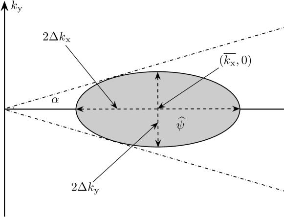
Figure 3: The essential numerical support of $\hat{\psi}.$

The pairs of widths $\Delta x,\Delta k_{\mathrm{x}}$ and $\Delta y,\Delta k_{\mathrm{y}}$ satisfy the Heisenberg uncertainty relation, which holds for any function $\psi$:

$$\Delta k_{\mathrm{x}}\,\Delta x\geq\frac{1}{2},\,\,\,\Delta k_{\mathrm{y}}\,\Delta y\geq\frac{1}{2}.$$ (42)

Equality holds only for the Morlet wavelet (see, for example [5]), which is the asymptotics of the Gaussian Wave Packet (12) as $p\to\infty$.

Our purpose here is to study the dependence of the widths and the means of the wavelet $\psi$ and the uncertainty relation on the parameters. Taking $\varepsilon$ as the unit of distance, we rewrite the wavelet in terms of the dimensionless coordinates $x^{\prime}=x/\varepsilon$, $y^{\prime}=y/\varepsilon,$ the time $t^{\prime}=t/\varepsilon,$ and two parameters $p$ and $\varepsilon/\gamma$ :

$$\frac{\psi(\boldsymbol{r}^{\prime})}{\sqrt{\varepsilon}}=\frac{(ps)^{\nu}K_{\nu}(ps)}{\sqrt{x^{\prime}+ct^{\prime}-i}},$$

$$s=\left[1-i\frac{\varepsilon}{\gamma}\left(x^{\prime}-ct^{\prime}+\frac{y^{\prime 2}}{x^{\prime}+ct^{\prime}-i}\right)\right]^{1/2}.$$ (43)

When $p$ is large, the parameter $p$ and the ratio $\varepsilon/\gamma$ can be interpreted with the help of the widths of the wavelet Morlet (36), which were denoted by $\sigma_{\mathrm{x}},\,\sigma_{\mathrm{y}},$ and the mean of the longitudinal spatial frequency of its Fourier transform, which is $\kappa.$ The ratio $\varepsilon/\gamma=\sigma_{\mathrm{y}}/\sigma_{\mathrm{x}}$ characterizes the shape of the essential numerical support of the wavelet, the product $\kappa\sigma_{\mathrm{x}}=\sqrt{p}$ is the number of wavelengths on the width $\Delta x,$ the product $\kappa\sigma_{\mathrm{y}}=\sqrt{\kappa\varepsilon/2}$ is the number of wavelengths on the width $\Delta y$.

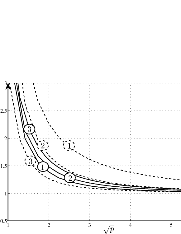
(a) Widths of the Gaussian Wave Packet $\psi(\boldsymbol{r})$ in relation to the widths of the Morlet wavelet, solid lines are for $\Delta x/\sigma_{\mathrm{x}}$, dashed lines are for $\Delta y/\sigma_{\mathrm{y}}$: line (1) is for $\varepsilon/\gamma=1/3$, line (2) is for $\varepsilon/\gamma=2/3$, line (3) is for $\varepsilon/\gamma=2$.

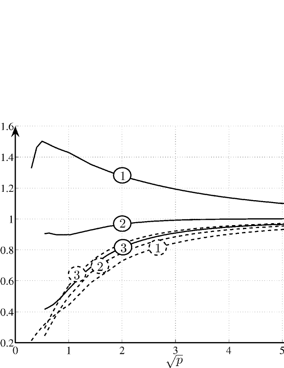
(b) Widths of the Fourier transform of the Gaussian Wave Packet $\widehat{\psi}(\boldsymbol{k})$ in relation to the widths of the Fourier transform of the Morlet wavelet, solid lines are for $\Delta k_{\mathrm{x}}/\sigma_{\mathrm{k}_{\mathrm{x}}}$, dashed lines are for $\Delta k_{\mathrm{y}}/\sigma_{\mathrm{k}_{\mathrm{y}}}$: line (1) is for $\varepsilon/\gamma=1/3$, line (2) is for $\varepsilon/\gamma=2/3$, line (3) is for $\varepsilon/\gamma=2$.

Figure 4: The ratios of the widths of the wavelet $\psi$ to the width of the Morlet wavelet are plotted versus $\sqrt{p}$ in spatial (a) and spatial frequency (b) domains for several values of $\varepsilon/\gamma.$

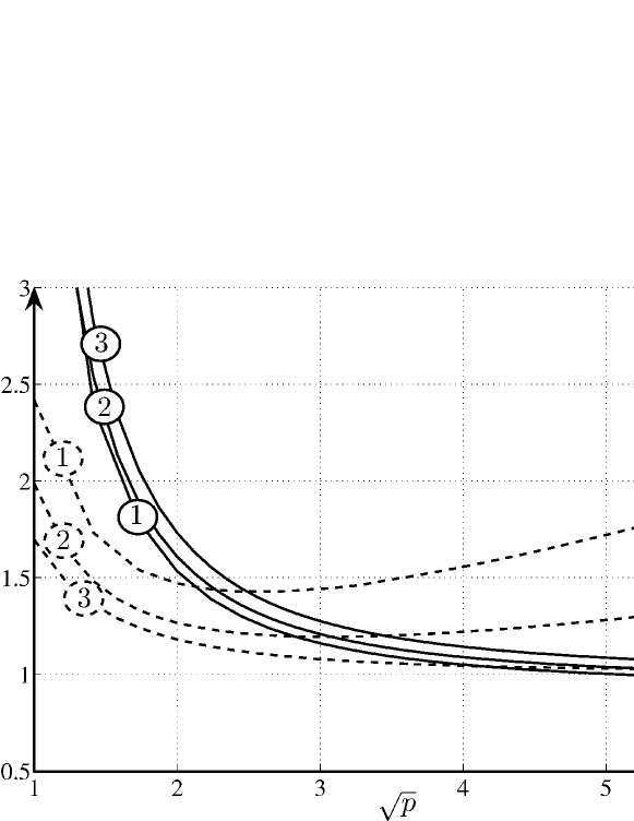
(a) Widths of the Gaussian Wave Packet $\psi(\boldsymbol{r})$ in relation to the widths of the Morlet wavelet, solid lines for $\Delta x/\sigma_{\mathrm{x}}$, dashed lines are for $\Delta y/\sigma_{\mathrm{y}}$: line (1) is for $2\kappa\varepsilon=4$, line (2) is for $2\kappa\varepsilon=8$, line (3) is for $2\kappa\varepsilon=64$.

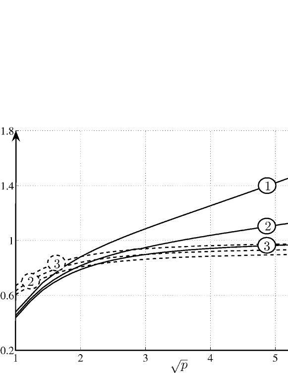
(b) Widths of the Fourier transform of the Gaussian Wave Packet $\widehat{\psi}(\boldsymbol{k})$ in relation to the widths of the Fourier transform of the Morlet wavelet, solid lines are for $\Delta k_{\mathrm{x}}/\sigma_{\mathrm{k}_{\mathrm{x}}}$, dashed lines are for $\Delta k_{\mathrm{y}}/\sigma_{\mathrm{k}_{\mathrm{y}}}$: line (1) is for $2\kappa\varepsilon=4$, line (2) is for $2\kappa\varepsilon=8$, line (3) is for $2\kappa\varepsilon=64$.

Figure 5: The relative widths of the wavelet $\psi$ are plotted versus $\sqrt{p}$ in spatial (a) and spatial frequency (b) domains for several values of $2\kappa\varepsilon$.

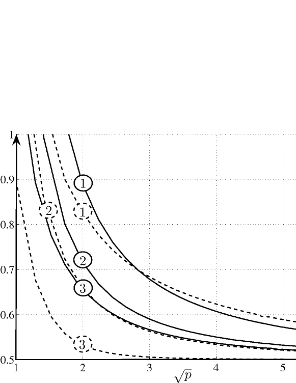
Figure 6: The left-hand side of the uncertainty relation for the Gaussian Wave Packet is plotted versus $\sqrt{p}$, solid lines are for $\Delta k_{\mathrm{x}}\Delta x$, dashed lines are for $\Delta k_{\mathrm{y}}\Delta y$: line (1) is for $\varepsilon/\gamma=1/3$, line (2) is for $\varepsilon/\gamma=2/3$, line (3) is for $\varepsilon/\gamma=2$.

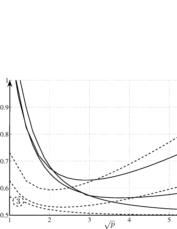
Figure 7: The left-hand side of the uncertainty relation for the Gaussian Wave Packet is plotted versus $\sqrt{p}$, solid lines are for $\Delta k_{\mathrm{x}}\Delta x$, dashed lines are for $\Delta k_{\mathrm{y}}\Delta y$: line (1) is for $2\kappa\varepsilon=4$, line (2) is for $2\kappa\varepsilon=8$, line (3) is for $2\kappa\varepsilon=64$.

We have calculated numerically the widths of the wavelet (12), its Fourier transforms, and the left-hand side of the uncertainty relations (42) as functions of $p=2\kappa\gamma$ in two cases. In the first case, the parameter $\kappa$ varies, the parameters $\varepsilon$ and $\gamma$ are kept constant. When $p$ is large, it can be interpreted as follows: the shape of the essential numerical support of the Morlet wavelet is kept constant and the number of wavelengths along the transverse and longitudinal widths increases with $\kappa.$ The results are plotted in Figures 4, 6. In the second case, $\gamma$ varies, the parameters $\varepsilon$ and $\kappa$ are kept constant. For large $p,$ this means that the number of wavelengths within the transverse width is kept fixed but the longitudinal width increases with increase of $\gamma$. The results are plotted in Figures 5, 7. In all cases, the number of wavelengths on the width $\Delta x,$ i.e., $\sqrt{p}$ is laid off along the horizontal axis. It is the parameter $\sqrt{p}$ that controls the asymptotic behavior of the new wavelet, because the correcting term in (36) is of order $O(1/\sqrt{p})$ when $\alpha={1\over 2}$. In view of comparing the widths with their asymptotics, the relatives widths, i.e., $\Delta_{\mathrm{x}}/\sigma_{\mathrm{x}},$ and so on, are plotted as ordinates in Figures 4, 5.

Figure 4 shows that all the widths tend to their asymptotic values as $\sqrt{p}\to\infty,$ the parameter $\varepsilon/\gamma$ being fixed. The widths of the wavelet in the coordinate domain are larger than their asymptotics $\sigma_{\mathrm{x}},$ $\sigma_{\mathrm{y}}$ (Figure 4a). The widths of the wavelet in the spatial frequency domain $\Delta k_{\mathrm{x}},$ $\Delta k_{\mathrm{y}}$ may be both smaller or larger than the same widths of the Morlet wavelet $\sigma_{\mathrm{k}_{\mathrm{x}}}=1/(2\sigma_{\mathrm{x}}),$   $\sigma_{\mathrm{k}_{\mathrm{y}}}=1/(2\sigma_{\mathrm{y}})$ (Figure 4b). The larger the parameter $\varepsilon/\gamma,$ the closer to the saturation the Heisenberg uncertainty relation (see Figure 6) and the smaller $\Delta\mathrm{y}/\sigma_{\mathrm{y}}$ (Figure 4a) and $\Delta\mathrm{k}_{\mathrm{x}}/\sigma_{\mathrm{k}_{\mathrm{x}}}$ ( Figure 4b). However $\Delta\mathrm{x}/\sigma_{\mathrm{x}}$ and $\Delta\mathrm{k}_{\mathrm{y}}/\sigma_{\mathrm{k}_{\mathrm{y}}}$ increase somewhat with increase in $\varepsilon/\gamma,$ remaining smaller than their counterparts.

To interpret Figures 5, 7, we note that the rate of convergence of the wavelet to the Morlet asymptotics is determined by terms of order $p^{-\alpha}\gamma/\varepsilon=(2\kappa)^{-\alpha}\gamma^{1-\alpha}/\varepsilon,$ which must be small. However these terms increase with $\gamma$ if $\varepsilon$ and $\kappa$ are fixed.

5.2 Directional properties of the wavelet $\psi$

A wavelet is called directional (see [5] for greater detail) if the essential numerical support of its Fourier transform lies in a convex cone in $\boldsymbol{k}$ space with its vertex at the origin and the angle $\alpha$ at the vertex (See Figure 3). Using the asymptotic formula (36), we can easily prove that the Gaussian Wave Packet is a directional wavelet when $p$ is large enough. This follows from the fact that $\overline{k_{\mathrm{x}}}=\kappa=p/(2\gamma)$, $\Delta k_{\mathrm{x}}=\sqrt{p}/(4\gamma)$ as $p\to\infty$, $\gamma$ and $\varepsilon$ are fixed. Thus the inequality $\overline{k_{\mathrm{x}}}>\Delta k_{\mathrm{x}}$ holds, which ensures that the origin lies outside the ellipse.

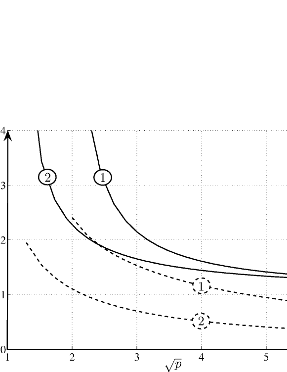
Figure 8: Scale and angle resolving powers for the Gaussian Wave Packet are plotted versus $\sqrt{p}$, solid lines are for the SRP, dashed lines are for ARP: line (1) is for $\varepsilon/\gamma=1/3$, line (2) is for $\varepsilon/\gamma=2$.

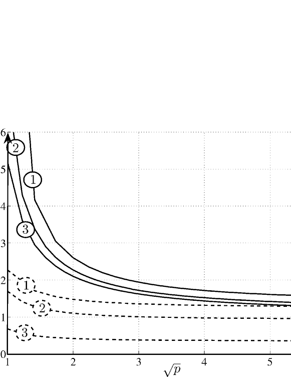
Figure 9: Scale and angle resolving powers for the Gaussian Wave Packet are plotted versus $\sqrt{p}$, solid lines are for the SRP, dashed lines are for ARP: line (1) is for $2\kappa\varepsilon=4$, line (2) is for $2\kappa\varepsilon=8$, line (3) is for $2\kappa\varepsilon=64$.

We can calculate numerically the scale resolving power (SRP) and the angular resolving power (ARP) if the wavelet is directional. These quantities are especially important for numerical calculations, mainly in determining the minimal sampling grid for a lossless reconstruction of the image (for more detail, see [3], [5]). The resolving powers are determined by the expressions

$$SPR(\psi)=\frac{\overline{k_{\mathrm{x}}}+\Delta k_{\mathrm{x}}}{\overline{k_{\mathrm{x}}}-\Delta k_{\mathrm{x}}}$$ (44)

$$APR(\psi)=2\,\mathrm{arccot}\frac{\sqrt{\left(\overline{k_{\mathrm{x}}}\right)^{2}-\left(\Delta k_{\mathrm{x}}\right)^{2}}}{\Delta{k_{\mathrm{y}}}}=\alpha.$$ (45)

As $SRP$ tends to $1$ and $ARP$ tends to $0$, the wavelet becomes more sensitive to small singularities and to angular details of the analyzed data [5]. The dependance of the angle and scale resolving powers was calculated by using MATLAB and is presented in Figure 8 and Figure 9 for the cases of varying $\kappa$ and $\gamma,$ respectively.

6 Multidimensional case

6.1 Definition and main properties

Here we give a generalization of the wavelets constructed in previous sections to the case of many spatial dimensions. The counterpart of (12) in $\mathbb{R}^{n}$ is

$$\psi(\boldsymbol{r})=\frac{\sqrt{2/\pi}\qquad(ps)^{\nu}K_{\nu}(ps)}{(x_{1}+ct-i\varepsilon_{2})^{1/2}(x_{1}+ct-i\varepsilon_{3})^{1/2}\cdot\ldots\cdot(x_{1}+ct-i\varepsilon_{\mathrm{n}})^{1/2}}$$ (46)

where $\boldsymbol{r}=(x_{1},x_{2},x_{3},\ldots,x_{\mathrm{n}}),$ $p$, $\gamma,$ $\varepsilon_{2},\ldots,\varepsilon_{\mathrm{n}}$ are positive parameters, the function $s$ is defined by (13), and it depends on $\boldsymbol{r},t,$ and on the parameters via $\theta,$ which is as follows:

$$\theta=x_{1}-ct+\frac{x_{2}^{2}}{x_{1}+ct-i\varepsilon_{2}}+\frac{x_{3}^{2}}{x_{1}+ct-i\varepsilon_{3}}+\ldots+\frac{x_{\mathrm{n}}^{2}}{x_{1}+ct-i\varepsilon_{\mathrm{n}}}.$$ (47)

If $t$ is time, the function $\psi(\boldsymbol{r})$ satisfies the wave equation

$$\psi_{tt}-c^{2}(\psi_{x_{1}x_{1}}+\psi_{x_{2}x_{2}}+\ldots+\psi_{x_{\mathrm{n}}x_{\mathrm{n}}})=0,\qquad c=\mathrm{const}.$$ (48)

If $\nu={1\over 2},$ formula (46) is transformed to an exact solution of (48), found in [24]:

$$\psi(\boldsymbol{r})=\frac{\exp{\left(-p\sqrt{1-{i\theta}/{\gamma}}\right)}}{(x_{1}+ct-i\varepsilon_{2})^{1/2}(x_{1}+ct-i\varepsilon_{3})^{1/2}\cdot\ldots\cdot(x_{1}+ct-i\varepsilon_{\mathrm{n}})^{1/2}}.$$ (49)

The exact solution (46) was mentioned in [19]. The Fourier transform of the wavelet (46) is found in the Appendix. It reads

$$\widehat{\psi}(\boldsymbol{k})=a_{n}\frac{p^{2\nu}}{\gamma^{\nu}}\left[k(k+k_{1})^{\nu+(n-1)/2}\right]^{-1}\times\\$$

$$\times\exp\left[-\frac{k+k_{1}}{2}\gamma-\frac{k_{2}^{2}\varepsilon_{2}+k_{3}^{2}\varepsilon_{3}+\ldots+k_{\mathrm{n}}^{2}\varepsilon_{\mathrm{n}}}{2(k+k_{1})}-\frac{2\kappa^{2}\gamma}{k+k_{1}}-ikct\right],$$ (50)

where $\boldsymbol{k}=(k_{1},k_{2},\ldots,k_{\mathrm{n}})$ is a wave vector, $k=|\boldsymbol{k}|,$

$$a_{n}=(2\pi)^{n/2}e^{i\pi(n-1)/4}.$$ (51)

The axially symmetric wavelet follows from (46), (47) if $\varepsilon_{2}=\varepsilon_{3}=\ldots=\varepsilon_{\mathrm{n}}\equiv\varepsilon.$ It reads

$$\psi(\boldsymbol{r})=\sqrt{\frac{2}{\pi}}\,\frac{(ps)^{\nu}K_{\nu}(ps)}{(x_{1}+ct-i\varepsilon)^{(n-1)/2}}.$$ (52)

Its Fourier transform is

$$\widehat{\psi}(\boldsymbol{k})=a_{n}\frac{p^{2\nu}}{\gamma^{\nu}}\left[k(k+k_{1})^{\nu+(n-1)/2}\right]^{-1}\times$$

$$\times\exp\left[-(k+k_{1})\frac{\gamma}{2}-(k-k_{1})\frac{\varepsilon}{2}-\frac{2\kappa^{2}\gamma}{k+k_{1}}-ikct\right].$$ (53)

All the properties of (12) are extended to (46) with minor corrections, i.e., it is a smooth function of coordinates, its moments of any order are zero. The same is true for its derivatives of any order with respect to coordinates and $t$. The modulus of (46) has a maximum at the point $x_{1}=ct,$ $x_{j}=0,j=2,\ldots,n.$ It has asymptotics (30) as $p\to\infty,$ where

$$\psi_{\mathrm{beam}}(\kappa,\boldsymbol{r})=\frac{\exp{(i\,\kappa\,\theta)}}{(x_{1}+ct-i\varepsilon_{2})^{1/2}\ldots(x_{1}+ct-i\varepsilon_{\mathrm{n}})^{1/2}},$$ (54)

which is uniform in the domain

$$\frac{x_{1}-ct}{\gamma}=O\left(\frac{1}{p^{\alpha}}\right),\qquad\frac{x_{j}}{\sqrt{\gamma\varepsilon_{j}}}=O\left(\frac{1}{p^{\alpha}}\right),\qquad j=2,3,...,n,$$ (55)

and ${1\over 3}\leq\alpha\leq{1\over 2}$. If the parameters $2ct/\varepsilon_{j},$ $p^{-\alpha}\gamma/\varepsilon_{j},\,j=2,..,n,$ are small, the asymptotics of the formula (30) with $\psi_{\mathrm{beam}}$ from (54) represents the Morlet wavelet

$$\psi(\boldsymbol{r})\sim\exp\left[i\kappa(x_{1}-ct)-\frac{(x_{1}-ct)^{2}}{2\sigma_{1}^{2}}-\frac{x_{2}^{2}}{2\sigma_{2}^{2}}\ldots-\frac{x_{\mathrm{n}}^{2}}{2\sigma_{\mathrm{n}}^{2}}\right]\times$$

$$\times\frac{C}{(-i\varepsilon_{2})^{1/2}(-i\varepsilon_{3})^{1/2}\ldots(-i\varepsilon_{\mathrm{n}})^{1/2}},$$ (56)

where $\sigma_{1}^{2}={4\gamma^{2}}/{p},$ $\sigma_{2}^{2}=\gamma\varepsilon_{2}/p,...$ $\sigma_{\mathrm{n}}^{2}=\gamma\varepsilon_{\mathrm{n}}/p$.

6.2 Coefficient $C_{\psi}$

For the usage of the Gaussian Wave Packet as a mother wavelet, we need to calculate the coefficient $C_{\psi}$ (for example, see [1], [5]) defined by the formula

$$C_{\psi}=\frac{1}{(2\pi)^{n}}\int\limits_{\mathbb{R}^{n}}d^{n}\boldsymbol{k}\frac{|\widehat{\psi}(\boldsymbol{k})|^{2}}{|\boldsymbol{k}|^{n}}.$$ (57)

Although we cannot calculate this integral analytically in the general case, we can simplify this expression. It should be noticed that

$$-\frac{(ic)^{n+1}}{n!}\int\limits_{-i\infty}^{0}dt\,t^{n}\,\exp(-ikct)=\frac{1}{k^{n+1}}.$$

This equation makes it possible to treat the integrand in (57) in the way

$$\frac{|\widehat{\psi}(\boldsymbol{k})|^{2}}{|\boldsymbol{k}|^{n}}=-\frac{e^{-i\pi(n-1)/4}}{(2\pi)^{n/2}}\frac{\gamma^{(n-1)/2}}{p^{n-1}}\frac{(ic)^{n+1}}{n!}\int\limits_{-i\infty}^{0}dt\,t^{n}\,\widehat{\psi}_{2}(\boldsymbol{k},t).$$ (58)

Here we denote the Gaussian Wave Packet with parameters $(\gamma,\varepsilon_{2},...\varepsilon_{\mathrm{n}},\kappa,\nu)$ by $\psi$ and the packet with parameters $(2\gamma,2\varepsilon_{2},...,2\varepsilon_{\mathrm{n}},\kappa,2\nu+(n-1)/2)$ by $\psi_{2}$. Then we can view the integral (57) as a Fourier inverse transform calculated at the point $\boldsymbol{r}=0$. Substituting the expression on the right-hand side of (58) into (57) and changing the order of integrals, we get

$$C_{\psi}=-\frac{e^{-i\pi(n-1)/4}}{(2\pi)^{n/2}}\frac{\gamma^{(n-1)/2}}{p^{n-1}}\frac{(ic)^{n+1}}{n!}\int\limits_{-i\infty}^{0}dt\,t^{n}\,\psi_{2}(0,t).$$ (59)

In the case where $n=3$ and $\varepsilon=\gamma,$ we can explicitly calculate the coefficient $C_{\psi}$ from the formula (57) if the coefficient $2\nu$ is a nonnegative integer. We calculate this integral in the spherical system of coordinates and use the integral representation of McDonald’s function $K_{\lambda}(z)$ (see [23]). We denote $k=|\boldsymbol{k}|$. As a result, we obtain

$$C_{\psi}=\int\limits_{\mathbb{R}^{3}}d^{3}\boldsymbol{k}\,\frac{|\widehat{\psi}(\boldsymbol{k})|^{2}}{|\boldsymbol{k}|^{3}}$$

$$=(2\pi)^{3}\frac{p^{4\nu}}{\gamma^{2\nu}}\int\limits_{\mathbb{R}^{3}}d^{3}\boldsymbol{k}\,\,\frac{1}{|\boldsymbol{k}|^{5}(|\boldsymbol{k}|+k_{\mathrm{x}})^{2\nu+2}}\exp\left[-2\gamma|\boldsymbol{k}|-\frac{4\kappa^{2}\gamma}{|\boldsymbol{k}|+k_{\mathrm{x}}}\right]$$

$$=(2\pi)^{4}\frac{p^{4\nu}}{\gamma^{4\nu}}\sum\limits_{m=0}^{2\nu}\,\frac{(2\nu)!}{m!}\,2^{-4\nu+m-1}\,\frac{\kappa^{-4\nu+m-5}}{\gamma^{-m+1}}\,K_{m+3}(4\kappa\gamma).$$ (60)

7 New wavelets and pulse complex sources

In previous sections, we discussed properties of a Gaussian packet viewed at a fixed moment of time as a wavelet. Now we are going to review properties of a Gaussian packet as a physical wavelet. The term ”physical wavelet” has been first suggested by G. Kaiser in [9]. These wavelets have been obtained as a sum of fields of two point sources with a special time dependence.

First we consider two wave equations with moving $\delta$-sources on the right-hand sides:

$$u^{\pm}_{tt}-c^{2}(u^{\pm}_{xx}+u^{\pm}_{yy})=\pm\phi(q,t)\delta(x+ct)\,\delta(y),$$

$$\phi(q,t)=A\sqrt{q}\exp(-2iqct),\qquad A=-e^{-i\pi/4}4\sqrt{\pi}c^{2}.$$ (61)

The equation, say, for $u^{+}$ can be solved if we seek a solution in the form

$$u^{+}(x,y,t)=\exp(iq\alpha)g(\beta,y),\qquad\alpha=x-ct,\qquad\beta=x+ct.$$ (62)

This leads to the Schrödinger equation for the function $g(\beta,y)$:

$$4iqg_{\beta}+g_{yy}=-4\sqrt{\pi}e^{-i\pi/4}\sqrt{q}\delta(\beta)\delta(y).$$ (63)

The solution of this equation is merely a well-known fundamental solution for the Schrödinger equation. So we get

$$u^{+}(\boldsymbol{r},t)=\frac{\Theta(x+ct)}{\sqrt{x+ct}}\exp\left[iq\left(x-ct+\frac{y^{2}}{x+ct}\right)\right],$$ (64)

where $\Theta$ is the Heaviside step function. We interpret it as a field of a source moving in the negative direction of the $x$ - axis at a speed $c,$ emitting an elementary pulse $\phi(q,t)$. The solution does vanish in front of the moving source, i.e., for $x<-ct,$ this is why it is called retarded. We denote the advanced solution, which does vanish behind the moving point, by $u^{-}$. It reads

$$u^{-}(\boldsymbol{r},t)=\frac{\Theta(-x-ct)}{\sqrt{x+ct}}\exp\left[iq\left(x-ct+\frac{y^{2}}{x+ct}\right)\right].$$ (65)

It can be interpreted as a field absorbed by the source moving in the negative direction of the $x$ - axis at a speed $c$ and producing the current $-\phi(t)$ in this source.

We note that $u=u^{+}+u^{-}$ is a sourceless solution, i.e., it satisfies the homogeneous wave equation, because $\Theta(x+ct)+\Theta(-x-ct)=1$. However, it has a singularity at the point $x=-ct$. In order to eliminate it, we shift $x$ by $-i\varepsilon/2,\,\,\varepsilon>0$ and $t$ by $-i\varepsilon/(2c)$ to the complex plane. This leads to a nonstationary Gaussian beam (31):

$$u(\boldsymbol{r},t)=\psi_{\mathrm{beam}}(q,\boldsymbol{r})=\frac{1}{\sqrt{x+ct-i\varepsilon}}\exp\left[iq\left(x-ct+\frac{y^{2}}{x+ct-i\varepsilon}\right)\right].$$ (66)

We get a Gaussian beam, using the sum of fields of moving sources, one of which emits and the other absorbs a pulse $\phi(q,t)$ that is proportional to $\exp(-2ictq).$ This result makes it possible to use an arbitrary function of time $t$ instead of an exponent on the right-hand side of (61), decomposing it into a Fourier integral. We apply

$$\Phi(t)=\int\limits_{0}^{\infty}dq\,\mathcal{F}(q)\,\phi(q,t)\equiv B\,\sigma^{\nu-1/2}K_{\nu-1/2}(\sigma),$$ (67)

$$\sigma=2\kappa\gamma(1+2ict/\gamma)^{1/2},\qquad B=-4c^{2}e^{-i\pi/4}\frac{p}{\sqrt{\gamma}},$$ (68)

$$\mathcal{F}(q)=a\,q^{-\nu-1}\,\exp\left[-\gamma\left(q+\frac{\kappa^{2}}{q}\right)\right]$$ (69)

instead of $\phi(q,t)$ as input source functions in (61) and obtain (12) instead of $\psi_{\mathrm{beam}}(q,\boldsymbol{r})$.

8 Conclusions

We suggest that we should consider an exponentially localized solution of the wave equation in several spatial dimensions, found earlier, from the point of view of continuous wavelet analysis. We investigate its properties as a mother wavelet and as a solution of the wave equation in view of its further application to the study of local properties and singularities of acoustic or optic fields.

We show that, depending on the parameters, the solution represents a short pulse of one oscillation, or a wave packet with the Gaussian envelop filled with oscillations, or a nonstationary Gaussian beam multiplied by a cutoff function.

The solution for a fixed time is a multidimensional wavelet with all zero moments. Its Fourier transform is calculated explicitly, and it is exponentially localized. The widths of the new wavelet in the position domain and in the spatial frequency domain, and the Heisenberg uncertainty relation are numerically investigated.

Appendix A Fourier transform of the Gaussian Wave Packet

A.1 Fourier transform of the two-dimensional packet

The Fourier transform of the wavelet (12) can be calculated using the Fourier decomposition of the Gaussian Wave Packet (12) in terms of the Gaussian beams (31) with the help of the formula

$$\psi(\boldsymbol{r})=\int\limits_{0}^{\infty}dq\,\mathcal{F}(q)\,\psi_{\mathrm{beam}}(q,\boldsymbol{r}).$$ (70)

To obtain this decomposition, we use the formula (see [23])

$$\sqrt{\frac{2}{\pi}}\,(ps)^{\nu}\,K_{\nu}(ps)=\int\limits_{0}^{\infty}dq\,\mathcal{F}(q)\,\exp(\,i\,q\,\theta),\\$$ (71)

$$\mathcal{F}(q)=a\,q^{-\nu-1}\,\exp\left[-\gamma\left(q+\frac{\kappa^{2}}{q}\right)\right],\\$$ (72)

$$a=\frac{1}{\sqrt{2\pi}}\frac{p^{2\nu}}{(2\gamma)^{\nu}},$$ (73)

where the left-hand side (71) depends on $\theta$ via $s$ from (13). We note that this relation is valid in the upper complex half-plane $\mathrm{Im}(\theta)>0,$ where $\theta$ lies when $x,y$ and time $t$ are real. Dividing both sides of (71) by the term $\sqrt{x+ct-i\varepsilon},$ we obtain (70). So the Fourier transform of the Gaussian Wave Packet is determined by the formula

$$\widehat{\psi}(\boldsymbol{k})=\int\limits_{0}^{\infty}dq\,\mathcal{F}(q)\,\widehat{\psi}_{\mathrm{beam}}(\boldsymbol{k},q).$$ (74)

The Fourier transform of the Gaussian beam (31) is found to be

$$\widehat{\psi}_{\mathrm{beam}}(\boldsymbol{k})=\int\limits_{\mathbb{R}^{2}}\,d^{2}\boldsymbol{r}\,\frac{\exp\left(-i\boldsymbol{k}\cdot\boldsymbol{r}\right)}{\sqrt{x+ct-i\varepsilon}}\exp\left[iq\left(x-ct+\frac{y^{2}}{x+ct-i\varepsilon}\right)\right]\\$$

$$=\int\limits_{-\infty}^{\infty}dx\,\exp(-ik_{\mathrm{x}}x)\,\,\exp[iq(x-ct)]\,I_{\mathrm{y}}(q,x),$$ (75)

where

$$I_{\mathrm{y}}(q,x)=\int\limits_{-\infty}^{+\infty}dy\,\frac{1}{\sqrt{x+ct-i\varepsilon}}\exp\left(-ik_{\mathrm{y}}y+iq\frac{y^{2}}{x+ct-i\varepsilon}\right)\,$$

$$=\sqrt{\frac{\pi}{q}}\,e^{i\pi/4}\,\exp\left[-i\frac{k_{\mathrm{y}}^{2}}{4q}(x+ct-i\varepsilon)\right].$$ (76)

Inserting (76) into (75), we obtain

$$\widehat{\psi}_{\mathrm{beam}}(\boldsymbol{k})=\int\limits_{-\infty}^{\infty}dx\,\exp(-ik_{\mathrm{x}}x)\,\exp\left[iq(x-ct)-i\frac{k_{\mathrm{y}}^{2}}{4q}(x+ct-i\varepsilon)\right]e^{i\pi/4}\sqrt{\frac{\pi}{q}}\\$$

$$=2\pi\,\exp{\left[-i\left(q+\frac{k_{\mathrm{y}}^{2}}{4q}\right)ct-\frac{k_{\mathrm{y}}^{2}\varepsilon}{4q}\right]}\,\delta\left(-k_{\mathrm{x}}+q-\frac{k_{\mathrm{y}}^{2}}{4q}\right)e^{i\pi/4}\sqrt{\frac{\pi}{q}}.$$ (77)

In view of further calculations of the integral with respect to $q,$ we modify the $\delta$ - function in (77). The roots of the argument of the $\delta$ - function, i.e., the roots of the equation

$$-k_{\mathrm{x}}+q-\frac{k_{\mathrm{y}}^{2}}{4q}=0$$ (78)

are $q_{1,2}=(k_{\mathrm{x}}\pm k)/2$, $k=|\boldsymbol{k}|.$ The negative root does not contribute to the integral, because ${\cal F}(q,\varepsilon)\equiv 0$ if $q<0.$ Taking into account the relations

$$\delta\left(-k_{\mathrm{x}}+q-\frac{k_{\mathrm{y}}^{2}}{4q}\right)=\frac{4q^{2}}{k_{\mathrm{y}}^{2}+4q^{2}}\,\delta\left(q-\frac{k_{\mathrm{x}}+k}{2}\right),$$ (79)

$$\frac{k_{\mathrm{y}}^{2}}{4q}+q=\frac{k^{2}-k_{\mathrm{x}}^{2}}{2(k+k_{\mathrm{x}})}+\frac{k+k_{\mathrm{x}}}{2}=k,\qquad\frac{4q^{2}}{k_{\mathrm{y}}^{2}+4q^{2}}=\frac{q}{k}=\frac{k_{\mathrm{x}}+k}{2k},$$ (80)

we obtain

$$\widehat{\psi}_{\mathrm{beam}}(\boldsymbol{k})=B(\boldsymbol{k})\,\delta\left(q-\frac{k_{\mathrm{x}}+k}{2}\right),$$ (81)

$$B(\boldsymbol{k})=2\pi\,\exp{\left(-ikct-\frac{k_{\mathrm{y}}^{2}\varepsilon}{2(k+k_{\mathrm{x}})}\right)}\,\frac{k+k_{\mathrm{x}}}{2k}e^{i\pi/4}\sqrt{\frac{2\pi}{k+k_{\mathrm{x}}}}.$$ (82)

After inserting (82) into (74), the integral disappears and the resulting expression contains $\mathcal{F}[(k+k_{\mathrm{x}})/2],$ which is as follows:

$$\mathcal{F}\left(\frac{k+k_{\mathrm{x}}}{2}\right)=a\;\frac{2^{\nu+1}}{(k+k_{\mathrm{x}})^{\nu+1}}\,\exp{\left(-\frac{k+k_{\mathrm{x}}}{2}\,\gamma\,-\,\frac{2\kappa^{2}\gamma}{k+k_{\mathrm{x}}}\right)}.$$ (83)

Taking into account

$$\frac{k_{\mathrm{y}}^{2}\varepsilon}{2(k+k_{\mathrm{x}})}=\frac{k-k_{\mathrm{x}}}{2}\varepsilon,$$ (84)

we obtain

$$\widehat{\psi}(\boldsymbol{k})=\mathcal{F}\left(\frac{k+k_{\mathrm{x}}}{2}\right)\,B(\boldsymbol{k}),$$

$$\widehat{\psi}(\boldsymbol{k})=2\pi\,e^{i\pi/4}\frac{p^{2\nu}}{\gamma^{\nu}}\,\left[k(k+k_{x})^{\nu+1/2}\right]^{-1}$$

$$\times\exp\left[-ikct-(k-k_{\mathrm{x}})\frac{\varepsilon}{2}-(k+k_{\mathrm{x}})\frac{\gamma}{2}-\frac{2\kappa^{2}\gamma}{k+k_{\mathrm{x}}}\right].$$ (85)

A.2 Fourier transform of a multidimensional Gaussian Wave Packet

In the multidimensional case, the Fourier transform of a Gaussian beam must be re-calculated. We put $\varepsilon_{2}\,=\,\varepsilon_{3}\,=\,...\,=\,\varepsilon_{\mathrm{n}}\,=\,\varepsilon$ from (46) for simplicity. Instead of $I_{\mathrm{y}},$ the formula (75) will contain the product $I_{\mathrm{x}_{2}}\cdot I_{\mathrm{x}_{3}}\ldots I_{\mathrm{x}_{\mathrm{n}}},$ where $n-1$ is the number of coordinates that are transverse to the direction of propagation. We obtain a formula for $I_{\mathrm{x_{k}}},$ $k=2,...,n,$ by replacing $y$ by $x_{\mathrm{k}}$ and $x$ by $x_{1}$ in (76). The analog of (77) will contain the sum $k_{2}^{2}+k_{3}^{2}+\ldots+k_{\mathrm{n}}^{2}=k^{2}-k_{1}^{2}$ instead of the term $k_{\mathrm{y}}^{2}=k^{2}-k_{\mathrm{x}}^{2},$ which does not yield any corrections and also the factor $\exp{(i\pi(n-1)/4)}\,(\pi/q)^{(n-1)/2}$ instead of such a factor for $n=2$. Therefore, (85) is modified as follows:

$$\widehat{\psi}(\boldsymbol{k})=A\,\left[k(k+k_{1})^{\nu+(n-1)/2}\right]^{-1}$$

$$\times\exp\left[-ikct-(k-k_{1})\frac{\varepsilon}{2}-(k+k_{1})\frac{\gamma}{2}-\frac{2\kappa^{2}\gamma}{k+k_{1}}\right],$$ (86)

where

$$A=(2\pi)^{n/2}\,\,e^{i(n-1)\pi/4}\,\frac{p^{2\nu}}{\gamma^{\nu}}.$$ (87)

References

- [1] Daubechies I 1992 Ten Lectures on Wavelets (Philadelphia, PA: SIAM)
- [2] Mallat S G 1999 A Wavelet Tour of Signal Processing, 2nd edn (San Diego, CA: Academic Press)
- [3] Antoine J - P, Murenzi R and Vandergheynst P 1996 Int. J. of Imaging Systems and Technology 7 152–65
- [4] Antoine J - P 2000 Revista Ciencias Matematicas(La Habana) 1 18
- [5] Antoine J - P, Murenzi R, Vandergheynst P and Ali S T 2004 Two-dimensional wavelets and their relatives (Cambridge: Cambridge University Press, UK)
- [6] Berg, van den J C (ed) 1999 Wavelets in Physics (Cambridge: Cambridge University Press)
- [7] Dahmen W 1997 Acta Numerica 6 55–228
- [8] Dahmen W 2001 J. Comp. Appl. Math. 128 133–85
- [9] Kaiser G 1994 A Friendly Guide to Wavelets, (Boston:Birkhäuser)
- [10] Visser M 2003 Phys. Let. A 315 219–24
- [11] Kaiser G 2003 J. Phys. A: Math. Gen., 36(30) R291-R338
- [12] Kaiser G 2004 J. Phys. A: Math. Gen., 37(22) 5929–47
- [13] Kaiser G 2005 J. Phys. A: Math. Gen., 38(2) 495-508
- [14] Murenzi R 1990 Ondelettes Multidimensionnelles et Applications à l’Analyse d’Images PhD Thesis Univ. Cath. Louvain Louvain-la-Neuve
- [15] Torresani B 1993 Some time-frequency aspects of continuous wavelet decompositions Progress in wavelet analysis and applications ed Y Meyer and S Roques (Editions Frontieres, 1993) pp 165–74
- [16] Deschenes S and Sheng Y 2002 Proc. of SPIE vol 4738 Wavelet and Independent Component Analysis Applications IX Harold H Szu and James R Buss (eds) pp. 372–81
- [17] Kiselev A P and Perel M V 1999 Optics and Spectroscopy 3 86
- [18] Kiselev A P and Perel M V 2000 J. Math. Phys 41(4) 1934–55
- [19] Perel M V and Fialkovsky I V 2003 J. of Math. Sc. 117(2) 3994-4000.
- [20] Perel M V and Sidorenko M S 2003 Wavelet Analysis in Solving the Cauchy Problem for the Wave Equation in Three-Dimensional Space In: Mathematical and numerical aspects of wave propagation: Waves 2003 Ed G C Cohen, E Heikkola et al (Springer-Verlag) pp 794–98.
- [21] Brittingham J 1983 J. Appl. Phys. 54 1179
- [22] Kiselev A P 1983 Radiophysics and Quantum Electron. 26(5) 755–61
- [23] Abramovitz M and Stegan I A (eds) 1970 Handbook of Mathematical Functions (Dover, New York, NY)
- [24] Kiselev A P and Perel M V 2000 Differential equations 4 41