A high accuracy Leray-deconvolution model of turbulence and its limiting behavior.

Abstract

In 1934 J. Leray proposed a regularization of the Navier-Stokes equations whose limits were weak solutions of the NSE. Recently, a modification of the Leray model, called the Leray-alpha model, has atracted study for turbulent flow simulation. One common drawback of Leray type regularizations is their low accuracy. Increasing the accuracy of a simulation based on a Leray regularization requires cutting the averaging radius, i.e., remeshing and resolving on finer meshes. This report analyzes a family of Leray type models of arbitrarily high orders of accuracy for fixed averaging radius. We establish the basic theory of the entire family including limiting behavior as the averaging radius decreases to zero, (a simple extension of results known for the Leray model). We also give a more technically interesting result on the limit as the order of the models increases with fixed averaging radius. Because of this property, increasing accuracy of the model is potentially cheaper than decreasing the averaging radius (or meshwidth) and high order models are doubly interesting.

MCS Classification : 76D05, 35Q30, 76F65, 76D03

Key-words : Navier-Stokes equations, Large eddy simulation, Deconvolution models.

1 Introduction

In 1934 J. Leray [Leray34a], [Leray34b] studied an interesting regularization of the Navier-Stokes equations (NSE). He proved that the regularized NSE has a unique, smooth, strong solution and that as the regularization length-scale $\delta\rightarrow 0$, the regularized system’s solution converges (modulo a subsequence) to a weak solution of the Navier-Stokes equations. This model has recently been attracting new interest as continuum model upon which large eddy simulation can be based (see, e.g., the work of Geurts and Holm [GH03] and Titi and co-workers [CHOT05], [CTV05], [VTC05]). If $\overline{\hbox{\bf w}}$ denotes a local spacial average of the velocity $\mathbf{w}$ associated with filter length-scale $\delta$ , the classical Leray model is given by

(1.1) $$\begin{array}[c]{l}\partial_{t}\hbox{\bf w}+\overline{\hbox{\bf w}}\cdot\nabla\hbox{\bf w}-\nu\triangle\hbox{\bf w}+\nabla q=\mathbf{f},\\ \nabla\cdot\hbox{\bf w}=0.\end{array}$$

Leray chose $\overline{\hbox{\bf w}}=g_{\delta}\star\hbox{\bf w}$, where $g_{\delta}$ is a Gaussian with averaging radius $\delta$. In $(\ref{Leray})$, $\nu$ is the kinematic viscosity, $(\hbox{\bf w},q)$ denotes the model’s velocity and pressure, $\Omega$ is the flow domain and $\mathbf{f}$ is the body force, assumed herein to be smooth and divergence free. We take $\Omega=(0,2\pi)^{3}$, the initial condition

$$\hbox{\bf w}(0,{\bf x})=\overline{\hbox{\bf u}}_{0}({\bf x})\quad\text{ in }\quad\Omega\text{\ ,}$$

and impose periodic boundary conditions (with zero mean) on the solution (and all problem data)

$$\hbox{\bf w}(t,{\bf x}+2\pi{\bf e}_{j})=\hbox{\bf w}(t,{\bf x})\quad\text{ and }\quad\int_{\Omega}\hbox{\bf w}(t,{\bf x})\,d{\bf x}=0.$$

The Leray model is easy to solve using standard numerical methods for the Navier-Stokes equations, e.g., [LMNR06], and, properly interpreted, requires no extra or ad hoc boundary conditions in the non-periodic case. However, as an LES model it has three main shortcomings:

• The Leray model’s solution can suffer an accumulation of energy around the cutoff frequency (Geurts and Holm [GH03]).

• The Gaussian filter is expensive to compute.

• The model $(\ref{Leray})$ has low accuracy on the smooth flow components, e.g., $||\hbox{\bf u}_{NSE}-\hbox{\bf w}||=O(\delta^{2})$ , Section 4.

The accumulation of energy around the cutoff length-scale can be ameliorated by new ideas in eddy viscosity which focus its effects on the smallest resolved scales or by time relaxation models with similar motivations, [Guer], [SAK01a], [SAK01b], [SAK02]. The expense of computing the filtered velocity is reduced (as proposed by Geurts and Holm [GH03]) if the Gaussian filter is replaced by a differential filter (introduced into LES by Germano [Ger86]). The resulting combination of Leray model plus differential filter, called the Leray-alpha model, has attracted an explosion of recent interest because of its theoretical clarity and computational convenience. For recent work on the Leray-alpha model, see Geurts and Holm [GH03], [GH05], Guermond and Prudhomme [GP05], Cheskidov, Holm, Olson and Titi [CHOT05], Ilyin, Lunasin and Titi [ILT05], Chepyzhov, Titi and Vishik [CTV05], [VTC05]  (among other works). Finally, there is the issue of the accuracy of $(\ref{Leray})$ upon the large scales / smooth flow components which must be improved if $(\ref{Leray})$ is to evolve from a descriptive regularization to a predictive model.

In this paper we complement the above work on $(\ref{Leray})$ by presenting the analysis of a new (and related) family of Leray-deconvolution models which have arbitrarily high orders of accuracy and include the Leray-alpha model as the zeroth order ($N=0$) case. To present the Leray-deconvolution models, some preliminaries are needed. Although any reasonable filter can be used, for definiteness, we fix the averaging to be by differential filter. Thus, given $2\pi$-periodic free divergence field w with zero mean value, its spacial average over $O(\delta)$ length-scales, denoted ${\overline{\hbox{\bf w}}}$, is the unique $2\pi$-periodic solution of the Stokes problem

(1.2) $$-\delta^{2}\triangle\overline{\hbox{\bf w}}+\overline{\hbox{\bf w}}+\nabla\pi=\hbox{\bf w}\quad\text{ in }\mathbb{R}^{3},\quad\nabla\cdot\overline{\hbox{\bf w}}=0,\quad\int_{\Omega}\overline{\hbox{\bf w}}=\mathbf{0}.$$

It can be shown that $\pi$ is a constant in the equation above and therefore the pressure term disappaers. Given a filter, the (ill-posed) deconvolution problem is then:

$$\text{given }\overline{\hbox{\bf w}},\text{ find a (useful and stable) {approximation }to }\hbox{\bf w}.$$

Let $D_{N}$ denote the map: $\overline{\hbox{\bf w}}\ \rightarrow$ chosen approximation to w, introduced in section 2. The approximate de-convolution operators, $N=0,1,2,\cdot\cdot\cdot$ , we consider have the asymptotic accuracy and stability properties (see Section 2)

(1.3) $$\phi=D_{N}\overline{\phi}+O(\delta^{2N+2})\text{ , for smooth }\phi\text{, }$$

(1.4) $$||D_{N}||_{\mathcal{L}(\mathbf{H}_{0}\rightarrow\mathbf{H}_{0})}\leq N+1<\infty,$$

where

(1.5) $$\mathbf{H}_{0}=\left\{\mathbf{v}\in L_{\hbox{\footnotesize loc}}^{2}({{\rm I}\hskip-2.0pt{\rm R}}^{3}),\quad 2\pi-\hbox{periodic},\quad\nabla\cdot\mathbf{v}=0,\quad\int_{\Omega}\mathbf{v}=\mathbf{0}\right\}.$$

The Leray-deconvolution model is then $\nabla\cdot\hbox{\bf w}=0$ and

(1.6) $$\partial_{t}\hbox{\bf w}+(D_{N}\overline{\hbox{\bf w}})\cdot\nabla\hbox{\bf w}-\nu\triangle\hbox{\bf w}+\nabla q=\mathbf{f}\quad\text{ in }\quad\mathbb{R}^{3}\times(0,T),\quad\int_{\Omega}\hbox{\bf w}=\mathbf{0},$$

subject to initial and $2\pi-$periodic boundary conditions. Because of $(\ref{EQ1})$, the formal accuracy of (1.4) on the smooth flow components as an approximation of the Navier-Stokes equations is $O(\delta^{2N+2}),N=0,1,2,\cdot\cdot\cdot$, Section 4. When $N=0$, $D_{0}\overline{\hbox{\bf w}}=\overline{\hbox{\bf w}}$ so $(\ref{Mod})$ reduces to the Leray-alpha regularization.

The behavior of the model as $N$ increases for $\delta$ fixed is beyond known Leray-type theories and relevant for practical computation. Indeed, decreasing $\delta$ for fixed $N$ requires reducing the computational meshwidth (a process which increases the storage and computing time dramatically) and resolving (1.1) or (1.2). On the other hand, increasing $N$ for $\delta$ fixed requires only the solution of one additional Poisson or Stokes-type problem per deconvolution step. The main theoretical contribution of this paper is, in Section 3, to resolve this limiting behavior of the model. We first prove existence and uniqueness of a smooth solution to $(\ref{Mod})$, then we show that (modulo a subsequence), for fixed $\delta$, as $N\rightarrow\infty$ the model solution $\hbox{\bf w}=\hbox{\bf w}(N)$ converges to a weak solution of the Navier-Stokes equations. To our knowledge, this is the first result on the limiting behavior of a family of turbulence models as the order of accuracy of a family of models on the large scales increases. The difference between the two limiting cases is, loosely speaking, that as $\delta\rightarrow 0$ , $\overline{\hbox{\bf w}}\rightarrow\hbox{\bf w}$ in every reasonable sense and the deconvolution process inherits this: $D_{N}\overline{\hbox{\bf w}}\rightarrow\hbox{\bf w}$ for $N$ fixed and as $\delta\rightarrow 0$. However, since deconvolution is ill-posed and the deconvolution operators $D_{N}$ are only an asymptotic (in $\delta$ for very smooth solutions and for $N$ fixed) inverse, the limiting behavior as $N\rightarrow\infty$ is more delicate.

Another new features include an $O(\delta^{2N+2})$ error bound for the energy norm of the model’s error (section 4): $||\hbox{\bf w}(\delta)-\hbox{\bf u}_{NSE}||$, provided the underlying solution of the Navier-Stokes equations is sufficiently smooth, and an estimate of the time averaged error $<||\nabla(\hbox{\bf u}_{NSE}-\hbox{\bf w})||_{H}^{2}>^{\frac{1}{2}}$ both for general weak solutions of the Navier-Stokes equations and for weak solutions having the $k^{-\frac{5}{3}}$ energy spectrum typical observed in fully developed turbulent flows. (These first of the two estimates is connected to related results for approximate deconvolution models in [LL06a], [LL06b], [LL03] and [DE06] and the second is an extension of the authors work in [LL06b].)

Of course, ultimately, practical computations require analytic guidance in balancing the computational meshwidth with $\delta$ , $N$ and other model and algorithmic parameters.

1.1 Notation and preliminaries

We use $||\cdot||$ to denote the $L^{2}(\Omega)$ norm and associated operator norm. We always impose the zero mean condition $\int_{\Omega}\phi dx=0$ on $\phi=\hbox{\bf w},p,\mathbf{f}$ and $\hbox{\bf w}_{0}$. Recall that

(1.7) $$\mathbf{H}_{0}=\left\{\mathbf{w}\in L^{2}_{\hbox{\footnotesize loc}}({{\rm I}\hskip-2.0pt{\rm R}}^{3}),\quad 2\pi-\hbox{periodic},\quad\nabla\cdot\mathbf{w}=0,\quad\int_{\Omega}\mathbf{w}=\mathbf{0}\right\}.$$

We also define the space function

(1.8) $$\mathbf{H}_{1}=\left\{\mathbf{w}\in H^{1}_{\hbox{\footnotesize loc}}({{\rm I}\hskip-2.0pt{\rm R}}^{3}),\quad 2\pi-\hbox{periodic},\quad\nabla\cdot\mathbf{w}=0,\quad\int_{\Omega}\mathbf{w}=\mathbf{0}\right\}.$$

We shall define the space $\mathbf{H}_{s}$ for every $s$ in the same way. We can thus expand the velocity in a Fourier series

$$\hbox{\bf w}(\mathbf{x},t)=\sum_{\mathbf{k}}\widehat{\hbox{\bf w}}(\mathbf{k},t)e^{-i\mathbf{k.x}},\text{ where }\mathbf{k}\in\mathbb{Z}^{3}\text{ is the wave-number.}$$

The Fourier coefficients are given by

$$\widehat{\hbox{\bf w}}(\mathbf{k},t)=\frac{1}{(2\pi)^{3}}\int_{\Omega}\hbox{\bf w}(x,t)e^{-i\mathbf{k.x}}d\mathbf{x.}$$

Magnitudes of $\mathbf{k}$ are defined by

$$|\mathbf{k}| =\{|k_{1}|^{2}+|k_{2}|^{2}+|k_{3}|\}^{\frac{1}{2}},$$

$$|\mathbf{k}|_{\infty} =\max\{|k_{1}|,|k_{2}|,|k_{3}|\}.$$

The length-scale of the wave number $\mathbf{k}$ is defined by $\displaystyle l=\frac{2\pi}{|\mathbf{k}|_{\infty}}.$ Parseval’s equality implies that the energy in the flow can be decomposed by wave number as follows. For $\hbox{\bf w}\in\mathbf{H}_{0}$ ,

$$\frac{1}{(2\pi)^{3}}\int_{\Omega}\frac{1}{2}|\hbox{\bf w}(x,t)|^{2}dx=\sum_{\mathbf{k}}\frac{1}{2}|\widehat{\hbox{\bf w}}(\mathbf{k},t)|^{2}=$$

$$=\sum_{k}\left(\sum_{k-1<|\mathbf{k|\leq}k}\frac{1}{2}|\widehat{\hbox{\bf w}}(\mathbf{k},t)|^{2}\right),\text{where }\mathbf{k}\in\mathbb{Z}^{3}\text{.}$$

Moreover, for $s\in{{\rm I}\hskip-2.0pt{\rm R}}$,

(1.9) $$\mathbf{H}_{s}=\left\{\mathbf{v}\in H^{s}_{\hbox{\footnotesize loc}}({{\rm I}\hskip-2.0pt{\rm R}}^{3}),\quad 2\pi-\hbox{periodic},\quad\nabla\cdot\mathbf{v}=0,\quad\widehat{\hbox{\bf w}}(\mathbf{0})=\mathbf{0},\quad\sum_{\mathbf{k}}|\mathbf{k}|^{2s}|\widehat{\hbox{\bf w}}(\mathbf{k},t)|^{2}<\infty\right\}.$$

We define the $\mathbf{H}_{s}$ norms by

(1.10) $$||\hbox{\bf w}||^{2}_{s}=\sum_{\mathbf{k}}|\mathbf{k}|^{2s}|\widehat{\hbox{\bf w}}(\mathbf{k},t)|^{2},$$

where of course $||\hbox{\bf w}||^{2}_{0}=||\hbox{\bf w}||^{2}$. It can be shown that when $s$ is an integer, $||\hbox{\bf w}||^{2}_{s}=||\nabla^{s}\hbox{\bf w}||^{2}$ (see [DG95]).

1.2 About the filter

Let $\hbox{\bf w}\in\mathbf{H}_{0}$ and $\overline{\hbox{\bf w}}\in\mathbf{H}_{1}$ be the unique solution to the Stokes problem.

(1.11) $$-\delta^{2}\triangle\overline{\hbox{\bf w}}+\overline{\hbox{\bf w}}+\nabla\pi=\hbox{\bf w}\quad\text{ in }\mathbb{R}^{3},\quad\nabla\cdot\overline{\hbox{\bf w}}=0,\quad\int_{\Omega}\overline{\hbox{\bf w}}=\mathbf{0}.$$

It is usual in deconvolution studies to denote the filtering operation by $G$ so that $\overline{\mathbf{w}}=G\mathbf{w}$. Writing

$$\hbox{\bf w}(\mathbf{x},t)=\sum_{\mathbf{k}}\widehat{\hbox{\bf w}}(\mathbf{k},t)e^{-i\mathbf{k.x}},$$

it is easily seen that $\nabla\pi=0$ and

(1.12) $$\overline{\hbox{\bf w}}(\mathbf{x},t)=\sum_{\mathbf{k}}{\frac{\widehat{\hbox{\bf w}}(\mathbf{k},t)}{1+\delta^{2}|\mathbf{k}|^{2}}}e^{-i\mathbf{k.x}}$$

Then writing $\overline{\hbox{\bf w}}=G(\hbox{\bf w})$, we see that in the corresponding spaces of the type $\mathbf{H}_{s}$, the transfer function of $G$, denoted by $\widehat{G}$ is the function

$$\widehat{G}(\mathbf{k})={\frac{1}{1+\delta^{2}|\mathbf{k}|^{2}}},$$

and we also can write on $\mathbf{H}_{s}$ spaces type

(1.13) $$-\delta^{2}\triangle\overline{\hbox{\bf w}}+\overline{\hbox{\bf w}}=\hbox{\bf w}\quad\text{ in }\mathbb{R}^{3},\quad\nabla\cdot\overline{\hbox{\bf w}}=0,\quad\int_{\Omega}\overline{\hbox{\bf w}}=\mathbf{0}.$$

Moreover, one notes that the transfer function depends only on the modulus of the wave vector $\mathbf{k}$. Therefore, by noting $k=|\mathbf{k}|$, we shall write in the following $\widehat{G}(k)$ instead of $\widehat{G}(\mathbf{k})$.

2 Approximate de-convolution operators

The de-convolution problem is central in image processing, [BB98]. The basic problem in approximate de-convolution is: given $\overline{\hbox{\bf w}}$ solve approximately for w:

(2.1) $$G\hbox{\bf w}=\overline{\hbox{\bf w}}.$$

Exact de-convolution is typically ill-posed. We consider the van Cittert [BB98] approximate de-convolution algorithm and associated operators, introduced into LES modeling by Adams, Kleiser and Stolz, e.g., [AS01], [AS02], [SA99], [SAK01a], [SAK01b], [SAK02]. For each $N=0,1,\cdot\cdot\cdot,$ $\hbox{\bf w}_{N}=D_{N}\overline{\hbox{\bf w}}$ is computed as follows.

Definition 2.1 (van Cittert approximate de-convolution algorithm)

Set $\hbox{\bf w}_{0}=\overline{\hbox{\bf w}}$,

for $n=1,2,\cdot\cdot\cdot,N-1$,

perform $\hbox{\bf w}_{n+1}=\hbox{\bf w}_{n}+\{\overline{w}-G\hbox{\bf w}_{n}\}$

Set $\hbox{\bf w}_{N}=D_{N}\overline{\hbox{\bf w}}$

By eliminating the intermediate steps, we find

(2.2) $$D_{N}\hbox{\bf w}=\sum_{n=0}^{N}(I-G)^{n}\hbox{\bf w}.$$

The approximate deconvolution operator $D_{N}$ is a bounded operator (Lemma 2.1) which approximates the unbounded exact deconvolution operator to high asymptotic accuracy $O(\delta^{2N+2})$ on subspaces of smooth functions (Lemma 2.2). We begin by summarizing from [DE06], [BIL06] a few important, known properties of the approximation deconvolution operator $D_{N}$ .

Lemma 2.1

[Stability of approximate de-convolution] Let the averaging be defined by $(\ref{FIT07})$ . Then $D_{N}$ is a self-adjoint, positive semi-definite operator on $\mathbf{H}_{0}$ and

$$||D_{N}||=N+1.$$

Lemma 2.2

[Error in approximate de-convolution] Let $G$ be given by the differential filter $(\ref{FIT07})$. For any $\hbox{\bf w}\in{\bf H}_{0},$

(2.3) $$\hbox{\bf w}-D_{N}\overline{\hbox{\bf w}} =(I-(-\delta^{2}\triangle+1)^{-1})^{N+1}\hbox{\bf w}$$

$$=(-1)^{N+1}\delta^{2N+2}\triangle^{N+1}(-\delta^{2}\triangle+1)^{-(N+1)}\hbox{\bf w}.$$

2.1 Some calculations

Since we consider the periodic problem, it is insightful visualize the approximate de-convolution operators $D_{N}$ in terms of the transfer function of the operator $\widehat{D_{N}}$ . Since these are functions of $\delta k$ , where $k=|\mathbf{k}|$, and not $\delta$ or $\mathbf{k}$, it is appropriate to record them re-scaled by

$$k\leftarrow\delta k.$$

Since $G=(-\delta^{2}\triangle+1)^{-1}$ , we find, after rescaling,  $\displaystyle\widehat{G}(k)=\frac{1}{1+k^{2}}$. With that, the transfer function of the first three deconvolution operators are

$$\widehat{D_{0}} =1,$$

$$\widehat{D_{1}} =2-\frac{1}{k^{2}+1}=\frac{2k^{2}+1}{k^{2}+1},\text{ and}$$

$$\widehat{D_{2}} =1+\frac{k^{2}}{k^{2}+1}+\left(\frac{k^{2}}{k^{2}+1}\right)^{2}.$$

These three are plotted together with the transfer function of exact de-convolution ($k^{2}+1$) (in bold).

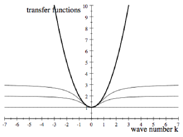
Figure 1: Exact and approximate ($N=0,1,2)$) de-convolution operators

More generally, we find

$$\widehat{D_{N}}(k):=\sum_{n=0}^{N}\left(\frac{1}{1+k^{2}}\right)^{n}=(1+k^{2})\left[1-\left(\frac{k^{2}}{1+k^{2}}\right)^{N+1}\right].$$

The large scales are associated with the wave numbers near zero (i.e., $|k|$ small). Thus, the fact that $D_{N}\$is a very accurate solution of the de-convolution problem for the large scales is reflected in the above graph in that the transfer functions have high order contact near $k=0$. The key observation in studying asymptotics of the model as $N\rightarrow\infty$ is that (loosely speaking) the region of high accuracy grows (slowly) as well as $N$ increases.

The regularization in the nonlinearity involves a special combination of averaging and deconvolution that we shall denote by $H_{N}$.

Definition 2.2

The truncation operator $H_{N}:\mathbf{H}_{0}\rightarrow\mathbf{H}_{0}$ is defined by

$$H_{N}\hbox{\bf w}:=D_{N}\overline{\hbox{\bf w}}=(D_{N}\circ G)\hbox{\bf w}.$$

Proposition 2.1

For each $N=0,1,\cdot\cdot\cdot$ , the operator $H_{N}$ is positive semi-definite on $\mathbf{H}_{0}$ . The operator $H_{N}:\mathbf{H}_{0}\rightarrow\mathbf{H}_{0}$ is a compact operator. Moreover, $H_{N}$ maps continuously $\mathbf{H}_{0}$ onto $\mathbf{H}_{2}$ . Further,

$$H_{N}\hbox{\bf w} =\overline{D_{N}\hbox{\bf w}},$$

$$||H_{N}||_{\mathcal{L}(\mathbf{H}_{0}\rightarrow\mathbf{H}_{0})} =1\text{ , for each }N\geq 0,$$

$$||H_{N}||_{\mathcal{L}(\mathbf{H}_{1}\rightarrow\mathbf{H}_{1})} =1\text{ , for each }N\geq 0.$$

Proof These properties are easily read off from the transfer function $\widehat{H}_{N}(k)$ of $H_{N}$ which we give next. For example, compactness follows since $|\widehat{H}_{N}(k)|\rightarrow 0$ as $|k|\rightarrow\infty$.

Remark 2.1

Similarly, by the same proof, $H_{N}$ maps $\mathbf{H}_{s}$ into itself (see Lemma 2.5 below), and is compact. Since $\left|\widehat{H}_{N}(k)\right|\leq 1$, one has for each $s\geq 0$

(2.4) $$||H_{N}\hbox{\bf w}||_{s}\leq||\hbox{\bf w}||_{s}.$$

The Fourier coefficients/transfer function of the operator $H_{N}$ are similarly easily calculated  to be (after rescaling by $k\leftarrow\delta k$)

(2.5) $$\widehat{H}_{N}(k)=1-\left(\frac{k^{2}}{1+k^{2}}\right)^{N+1}.$$

They are plotted below for a few values of $N$.

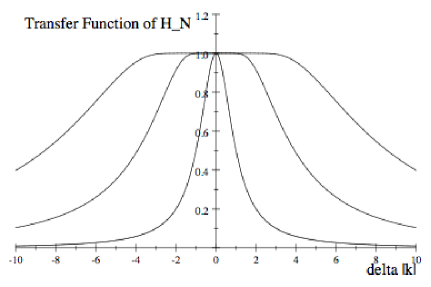
Figure 2: Transfer function of $H_{N}$, $N=0,10,50)$

These plots are representative of the behavior of the whole family. Examining the above graphs, we observe that $H_{N}(u)$ is very close to $u$ for the low frequencies/largest solution scales and that $H_{N}(u)$ attenuates small scales/high frequencies. The breakpoint between the low frequencies and high frequencies is somewhat arbitrary. The following (from [LN06a]) is convenient for our purposes and fits our intuition of an approximate spectral cutoff operator. We take for $k_{c}$ the frequency for which $\widehat{H}_{N}$ most closely attains the value $\frac{1}{2}.$

Definition 2.3 (Cutoff-Frequency)

The cutoff frequency of $H_{N}$ is

$$k_{c}:=\text{greatest integer}\left(\widehat{H}_{N}^{-1}\left(\frac{1}{2}\right)\right).$$

In other words, the frequency for which $\widehat{H}_{N}$ most closely attains the value $\frac{1}{2}.$

From the above explicit formulas, it is easy to verify that the cutoff frequency grows to infinity slowly as $N\rightarrow\infty$ for fixed $\delta$ and as $\delta\rightarrow 0$ for fixed $N$. Other properties (whose proofs are simple calculations) of the operator $H_{N}(\cdot)$ follow similarly easily from $\displaystyle\widehat{H}_{N}(k)=1-\left(\frac{k^{2}}{1+k^{2}}\right)^{N+1}$.

Lemma 2.3

For all $N\geq 0,$ $\widehat{H}_{N}(k)$ has the following properties:

$$0 <\widehat{H}_{N}(k)\leq 1,$$

$$|\widehat{H}_{N}(k)| \rightarrow 0\text{ as }|k|\rightarrow\infty,$$

$$\widehat{H}_{N}(0) =1.$$

Let $k_{c}$ be cutoff frequency, then

$$|k_{c}|\rightarrow\infty\text{ as }N\rightarrow\infty\text{ for fixed }\delta\text{ and as }\delta\rightarrow 0\text{ for }N\text{ fixed.}$$

For any fixed value of $k$ (or bounded set of values of $k$ )

$$\widehat{H}_{N}(k)\rightarrow 1\text{ as }N\rightarrow\infty\ \text{\ for }\delta\ \text{fixed and as }\delta\rightarrow 0\text{ \ for }N\ \text{fixed}$$

Proof. This follows from $(\ref{TRAN00})$.

To extract strong convergence of deconvolution, some restriction to the large scales is needed (as shown clearly in the above two figures). One way to do this is to consider the action of deconvolution operators on trigonometric polynomials.

Definition 2.4

The space  $\mathbf{I}\!\mathbf{P}_{n}$ denotes the $2\pi$-periodic, divergence-free, wit hzero mean value, vector, trigonometric polynomials of degree $\leq n$  and $\Pi_{n}:\mathbf{H}_{0}\rightarrow\mathbf{I}\!\mathbf{P}_{n}$  is the associated orthogonal projection.

The model error is driven by the error in approximate deconvolution. With this definition a critical convergence result on approximate deconvolution is possible.

Proposition 2.2

$H_{N}$ is a compact, symmetric positive semi-definite operator. For $n$ fixed, $H_{N}$ is strictly positive definite on $\mathbf{I}\!\mathbf{P}_{n}$ and

$$H_{N}\rightarrow I\text{ on }\mathbf{I}\!\mathbf{P}_{n}\text{ in the strong operator norm on }\mathbf{H}_{0}\text{.}$$

Given  $n$  there is an $N_{0}(n)$ large enough such that

$$||\Pi_{n}\mathbf{v}||\leq 2||H_{N}^{\frac{1}{2}}\mathbf{v}||\text{ , for all }N\geq N_{0}(n),$$

Further,

$$||\mathbf{v}||\leq||H_{N}^{\frac{1}{2}}\mathbf{v}||\leq 2||\mathbf{v}||\text{ for all }\,\,\mathbf{v}\in P_{n}\text{.}$$

Proof. This follows from $(\ref{TRAN00})$. For example, Compactness follows since $\widehat{H}_{N}(k)\rightarrow 0$ as $k\rightarrow\infty.$

Other properties of the operator $H_{N}(\cdot)$ follow similarly easily from its transfer function.

Proposition 2.3

Let $\Pi_{k_{c}}$ denote the orthogonal $\mathbf{H}_{0}$ projection into

$span\{e^{i\mathbf{k\cdot x}}:|\mathbf{k}|\leq k_{c}\}.$ For all $\hbox{\bf w}\in\mathbf{H}_{0}$:

(2.6) $$(H_{N}\hbox{\bf w},\hbox{\bf w}) \geq C||\Pi_{k_{c}}\hbox{\bf w}||^{2},$$

$$(\hbox{\bf w}-H_{N}\hbox{\bf w},\hbox{\bf w}) \geq C||(I-\Pi_{k_{c}})\hbox{\bf w}||^{2}.$$

Proof  The claims follow from the definition of the cutoff frequency, the explicit formula for the transfer function and direct calculation.

The following properties are important to the analysis that follows.

Lemma 2.4

Let $s\in{{\rm I}\hskip-2.0pt{\rm R}}$, $\hbox{\bf w}\in\mathbf{H}_{s}$. Then $H_{N}(\hbox{\bf w})\in\mathbf{H}_{s+2}$.

Proof. Since $H_{N}(\hbox{\bf w})$ satisfies periodic boundary conditions, it is divergence free and has zero mean value by construction. We check the regularity. It is easy checked by using a Taylor expansion that there exists a constant $C=C(\delta,N)$ such that

(2.7) $$\forall\,\mathbf{k}\,\in\mathbb{Z}^{3},\,\mathbf{k}\not=0,\quad 0\leq\hat{H}_{N}(k)\leq{\frac{C(\delta,N)}{k^{2}}},\quad\hbox{with }k=\mathbf{k}.$$

Therefore, for $\hbox{\bf w}\in\mathbf{H}_{s}$, $\hbox{\bf w}(\mathbf{x})=\sum_{\mathbf{k}\in\mathbb{Z}}\widehat{\hbox{\bf w}}(\mathbf{k})e^{-i\mathbf{k\cdot x}}$

(2.8) $$(\widehat{H}_{N}(k))^{2}k^{2(s+2)}|\hbox{\bf w}(\mathbf{k})|^{2}\leq C(\delta,N)^{2}k^{2s}|\hbox{\bf w}(\mathbf{k})|^{2}.$$

Recall that here $\widehat{\hbox{\bf w}}(\mathbf{0})=\mathbf{0}$. Therefore in $(\ref{241106})$, $k\not=0$. Hence, by definition

(2.9) $$||H_{N}(\hbox{\bf w})||_{\mathbf{H}_{s+2}}\leq C(\delta,N)||\hbox{\bf w}||_{\mathbf{H}_{s}},$$

and the proof is finished.

Remark 2.2

The constant $C(\delta,N)$ in the above proof blows up as $\delta\rightarrow 0$ or as $N\rightarrow\infty$.

Lemma 2.5

1) The operator $H_{N}$ maps continuously $\mathbf{H}_{s}$ into $\mathbf{H}_{s}$ and

(2.10) $$||H_{N}||_{\mathcal{L}(\mathbf{H}_{s},\mathbf{H}_{s})}=1.$$

2) For every $\hbox{\bf w}\in\mathbf{H}_{s}$, $H_{N}(\hbox{\bf w})$ converges strongly to w in $\mathbf{H}_{s}$ when $N\rightarrow\infty$.

3) $H_{N}$ commutes with the gradient operator: $\nabla H_{N}=H_{N}\nabla$.

Proof. 1) Let $\hbox{\bf w}=(w^{1},w^{2},w^{3})\in\mathbf{H}_{s}$. One has

$$||\hbox{\bf w}||_{s}^{2}=\sum_{\mathbf{k}\in\mathbb{Z}^{3}}k^{2s}|\widehat{w}(\mathbf{k})|^{2}.$$

Let us note $\widehat{w}(\mathbf{k})=(w_{\mathbf{k}}^{1},w_{\mathbf{k}}^{2},w_{\mathbf{k}}^{3})$, $H_{N}(\hbox{\bf w})=(H_{N}(\hbox{\bf w})^{1},H_{N}(\hbox{\bf w})^{2},H_{N}(\hbox{\bf w})^{3})$. Therefore, the $j^{\hbox{\footnotesize th}}$ component of the vector field $H_{N}(\hbox{\bf w})$ is given by

(2.11) $$H_{N}(\hbox{\bf w})^{j}=\sum_{\mathbf{k}\in\mathbb{Z}^{3}}\widehat{H}_{N}(k)w_{\mathbf{k}}^{j}e^{i\mathbf{k}.\mathbf{x}}.$$

Consequently

$$\nabla\cdot H_{N}(\hbox{\bf w})=\sum_{\mathbf{k}\in\mathbb{Z}^{3}}i\widehat{H}_{N}(k)k_{j}w_{\mathbf{k}}^{j}e^{i\mathbf{k}.\mathbf{x}}.$$

When $\hbox{\bf w}\in\mathbf{H}_{1}$, $\forall\,\mathbf{k}\in\mathbb{Z}^{3}$, $k_{j}w_{\mathbf{k}}^{j}=0$. Then $\nabla\cdot H_{N}(\hbox{\bf w})=0$. Now recall that

$$\widehat{H}_{N}(k)=1-\left({\frac{k^{2}}{1+k^{2}}}\right)^{N+1}.$$

One deduces that $|\hat{H}_{N}(k)|\leq 1$ and

$$k^{2s}|\hat{H}_{N}(k)\widehat{w}(\mathbf{k})|^{2}\leq k^{2s}|\widehat{w}(\mathbf{k})|^{2}$$

yielding $||H_{N}(\hbox{\bf w})||_{s}\leq||\hbox{\bf w}||_{s}$. Hence

$$H_{N}(\hbox{\bf w})\in\mathbf{H}_{s}\quad\hbox{and}\quad||H_{N}(\hbox{\bf w})||_{\mathbf{H}_{s}}\leq||\hbox{\bf w}||_{\mathbf{H}_{s}},$$

showing $||H_{N}||_{\mathcal{L}(\mathbf{H}_{s},\mathbf{H}_{s})}\leq 1$. Now let $\mathbf{k}=(k_{1},k_{2},0)\in\mathbb{Z}$, $k_{1}\not=0$, $k=|\mathbf{k}|$ and define

$$\widehat{\mathbf{w}}(\mathbf{k})={\frac{1}{k^{s}\sqrt{1+(k_{2}/k_{1})^{2}}}}(1,-(k_{2}/k_{1}),0),\quad\hbox{\bf w}_{\mathbf{k}}(\mathbf{x})=\widehat{\mathbf{w}}(\mathbf{k})e^{i\mathbf{k}.\mathbf{x}}.$$

By construction $\hbox{\bf w}_{\mathbf{k}}\in\mathbf{H}_{s}$, $||\hbox{\bf w}_{\mathbf{k}}||_{\mathbf{H}_{s}}=1$, and one also has $||H_{N}\hbox{\bf w}_{\mathbf{k}}||_{\mathbf{H}_{s}}=\widehat{H}_{N}(k)\rightarrow 1$ as $k$ $\rightarrow\infty$, making sure that $||H_{N}||_{\mathcal{L}(\mathbf{H}_{s},\mathbf{H}_{s})}=1$.

2) Let $\hbox{\bf w}\in\mathbf{H}_{s}$. One has

$$||\hbox{\bf w}-H_{N}\hbox{\bf w}||_{s}=\sum_{\mathbf{k}\in\mathbb{Z}^{3}}\left({\frac{k^{2}}{1+k^{2}}}\right)^{2(N+1)}k^{2s}|\widehat{\hbox{\bf w}}(\mathbf{k})|^{2}$$

Let $\varepsilon>0$. Since $\hbox{\bf w}\in\mathbf{H}_{s}$, there exists $K>0$ such that

$$\sum_{k\geq K}k^{2s}|\widehat{\hbox{\bf w}}(\mathbf{k})|^{2}\leq{\frac{\varepsilon}{2}},$$

yielding

$$||\hbox{\bf w}-H_{N}\hbox{\bf w}||_{s}\leq\left({\frac{K^{2}}{1+K^{2}}}\right)^{2(N+1)}||\hbox{\bf w}||_{s}+{\frac{\varepsilon}{2}}$$

Now, as $K>0$, $K^{2}/(1+K^{2})<1$, there exists $N_{0}$ (which depends upon w) such that $\forall\,N\geq N_{0}$,

$$\left({\frac{K^{2}}{1+K^{2}}}\right)^{2(N+1)}||\hbox{\bf w}||_{s}\leq{\frac{\varepsilon}{2}}.$$

Then $\forall\,N\geq N_{0}$, $||\hbox{\bf w}-H_{N}\hbox{\bf w}||_{\mathbf{H}_{s}}\leq\varepsilon$. This shows the strong $\mathbf{H}_{s}$ convergence of $H_{N}\hbox{\bf w}$ to w as $N$ $\rightarrow\infty$.

3) The fact that $H_{N}$ commutes with $\nabla$ is obvious.

Remark 2.3

All the results in Lemma 2.5 above are uniform in $\delta$. Moreover, it easy checked that for a fixed $N$, the same convergence result holds when $\delta$ goes to zero.

Remark 2.4

Let $\hbox{\bf w}\in L^{2}([0,T],\mathbf{H}_{s})$. It easy checked by using the same proof as in Lemma 2.5 combined with the Lebesgue monotone convergence theorem that $H_{N}(\hbox{\bf w})$ converges to w in $L^{2}([0,T],\mathbf{H}_{s})$ as $N$ goes to infinity.

3 The Leray Deconvolution Model

3.1 Existence result

The theory of Leray-deconvolution model begins, like the Leray theory of the Navier-Stokes equations, with a clear global energy balance, and existence and uniqueness of solutions.

Let $\hbox{\bf u}_{0}\in\mathbf{H}_{0}$, $f\in\mathbf{H}_{-1}$. For $\delta>0$, let the averaging be defined by $(\ref{filter})$. The problem we consider is the following, for a fixed $T>0$, find $(\hbox{\bf w},q)$

(3.1) $$\left\{\begin{array}[c]{l}\hbox{\bf w}\in L^{2}([0,T],\mathbf{H}_{1})\cap L^{\infty}([0,T],\mathbf{H}_{0}),\quad\partial_{t}\hbox{\bf w}\in L^{2}([0,T],\mathbf{H}_{-1})\\ q\in L^{2}([0,T],L^{2}_{{\hbox{\footnotesize per},0}}),\\ \partial_{t}\hbox{\bf w}+(H_{N}(\hbox{\bf w})\nabla)\hbox{\bf w}-\nu\triangle\hbox{\bf w}+\nabla q=H_{N}(\mathbf{f})\quad\text{ in }\mathbb{\mathcal{D}}^{\prime}([0,T]\times{{\rm I}\hskip-2.0pt{\rm R}}^{3}),\\ \hbox{\bf w}(\mathbf{x},0)=H_{N}(\hbox{\bf u}_{0})=\hbox{\bf w}_{0}.\end{array}\right.$$

where $L^{2}_{{\hbox{\footnotesize per},0}}$ denotes the scalar fields in $L^{2}_{loc}({{\rm I}\hskip-2.0pt{\rm R}}^{3})$, $2\pi$-periodic with zero mean value.

Theorem 3.1

The problem $(\ref{pb})$ admits a unique solution $(\hbox{\bf w},q)$, where w satisfies the energy equality

(3.2) $$\frac{1}{2}\left\|\hbox{\bf w}(t)\right\|^{2}+\nu\int_{0}^{t}\int_{\Omega}|\nabla\hbox{\bf w}|^{2}d{\bf x}dt^{\prime}=\frac{1}{2}\left\|H_{N}(\hbox{\bf u}_{0}\right\|^{2}+\int_{0}^{t}\int_{\Omega}H_{N}(\mathbf{f}).\hbox{\bf w}\,d{\bf x}dt^{\prime}.$$

Moreover, $\hbox{\bf w}\in L^{\infty}([0,T],\mathbf{H}_{1})\cap L^{2}([0,T],\mathbf{H}_{2})$

Proof. For simplification, one notes $||\cdot||_{p,B}$ the norm in $L^{p}([0,T],B)$ and when $B=\mathbf{H}_{s}$ one shall note $||\cdot||_{p,s}$ for the simplicity. One also considers the space

(3.3) $$\mathbf{V}=L^{2}([0,T],\mathbf{H}_{1})\cap L^{\infty}([0,T],\mathbf{H}_{0}),\quad||\hbox{\bf w}||_{\mathbf{V}}=||\hbox{\bf w}||_{2,1}+||\hbox{\bf w}||_{\infty,0}.$$

Recall that (see [Le06]),

(3.4) $$\forall\hbox{\bf w}\in\mathbf{V},\quad\forall\,r\in[2,6],\quad||\hbox{\bf w}||_{{\frac{4r}{3(r-2)}},L^{r}}\leq C||\hbox{\bf w}||_{V}.$$

We introduce the operators:

(3.5) $$\begin{array}[c]{l}\displaystyle A(\hbox{\bf w},\hbox{\bf v})=\nu\int_{0}^{T}\int_{\Omega}\nabla\hbox{\bf w}.\nabla\hbox{\bf v},\\ \displaystyle B_{N}(\hbox{\bf w},\hbox{\bf v})=\int_{0}^{T}\int_{\Omega}(H_{N}(\hbox{\bf w})\nabla)\hbox{\bf w}.\hbox{\bf v}=-\int_{0}^{T}\int_{\Omega}H_{N}(\hbox{\bf w})\otimes\hbox{\bf w}:\nabla\hbox{\bf v}.\end{array}$$

We first notice that

(3.6) $$|A(\hbox{\bf w},\hbox{\bf v})|\leq\nu||\hbox{\bf w}||_{2,1}||\hbox{\bf v}||_{2,1}.$$

Now assume that $\hbox{\bf w}\in V$, $\hbox{\bf v}\in L^{2}([0,T],\mathbf{H}_{1})$. Using lemma 2.4 combined with an integration by parts and the Sobolev Theorem, it is easy seen that there exits a constant $C$ which depends on $N$ and such that one has

(3.7) $$|B_{N}(\hbox{\bf w},\hbox{\bf v})|\leq C||\hbox{\bf w}||_{V}^{2}||\hbox{\bf v}||_{2,1},\quad B_{N}(\hbox{\bf w},\hbox{\bf w})=0.$$

Here we have remarked that because $\mathbf{H}_{2}\subset(L^{\infty}({{\rm I}\hskip-2.0pt{\rm R}}))^{3}$ (we are working in a 3D configuration), $\hbox{\bf w}\in L^{\infty}([0,T],\mathbf{H}_{0})$ yields $H_{N}(\hbox{\bf w})\in L^{\infty}([0,T],\mathbf{H}_{2})$ (see $(\ref{BOOF})$) and therefore,

(3.8) $$H_{N}(\hbox{\bf w})\in L^{\infty}([0,T]\times{{\rm I}\hskip-2.0pt{\rm R}}),\quad||H_{N}(\hbox{\bf w})||_{\infty,L^{\infty}}\leq C||\hbox{\bf w}||_{V}$$

for a constant $C$ which depends on $N$. We now note

(3.9) $$\mathbf{W}=\{\hbox{\bf w}\in\mathbf{V},\,\,\partial_{t}\hbox{\bf w}\in L^{2}([0,T],\mathbf{H}_{-1})\}.$$

Notice that any $\hbox{\bf w}\in\mathbf{W}$ is almost every-where equal to a function in $C^{0}([0,T],\mathbf{H}_{0})$ (see in [RT84]). Therefore, passing to a quotient space by keeping the same notations, we have

$$\mathbf{W}\subset C^{0}([0,T],\mathbf{H}_{0}).$$

Finally when $\mathbf{f}\in L^{2}([0,T],\mathbf{H}_{-1})$, then $H_{N}(\mathbf{f})\in L^{2}([0,T],\mathbf{H}_{1})$ and the variational formulation of Problem $(\ref{pb})$ is:

(3.10) $$\begin{array}[c]{l}\hbox{Find }\hbox{\bf w}\in\mathbf{W}\quad\hbox{such that}\quad\hbox{\bf w}(0,\mathbf{x})=\hbox{\bf w}_{0},\quad\hbox{and}\quad\forall\,\hbox{\bf v}\in L^{2}([0,T],\mathbf{H}_{1}),\\ \displaystyle\int_{0}^{T}<\partial_{t}\hbox{\bf w},\hbox{\bf v}>+B_{N}(\hbox{\bf w},\hbox{\bf v})+A(\hbox{\bf w},\hbox{\bf v})=\int_{0}^{T}\int_{\Omega}H_{N}(\mathbf{f}).\hbox{\bf v}\,d{\bf x}dt\end{array}$$

Since $(\ref{POUF})$ and $(\ref{POUPOUF})$ are satisfied, the existence of a solution to Problem $(\ref{MEUH})$ can be derived thanks to the Galerkin method. This is classical and the reader can look at [LLe06] and references inside or also in [RT84] for a detailed descrition of such kind of proof. By taking $\hbox{\bf w}=\hbox{\bf v}$ as test vector field in $(\ref{MEUH})$ (a legal operation here), one directly gets the energy estimate $(\ref{ENER})$. Notice that thanks to the energy equality and $||H_{N}(\hbox{\bf u}_{0})||\leq||\hbox{\bf u}_{0}||$, $||H_{N}(\mathbf{f})||_{-1}\leq||\mathbf{f}||_{-1}$, w does satisfy the following estimates:

(3.11) $$||\hbox{\bf w}||_{\infty,0}^{2}\leq||\hbox{\bf w}_{0}||^{2}+{\frac{1}{\nu}}||\mathbf{f}||_{2,-1}^{2},\quad||\hbox{\bf w}||_{2,1}^{2}\leq{\frac{1}{\nu}}||\hbox{\bf w}_{0}||^{2}+{\frac{1}{\nu^{2}}}||\mathbf{f}||_{2,-1}^{2}$$

in other words,

(3.12) $$||\hbox{\bf w}||_{V}\leq C(\nu,||\hbox{\bf u}_{0}||,||\mathbf{f}||_{2,-1}).$$

Here the bound does not depend on $N$. Notice also that we can derive an estimate for $\partial_{t}\hbox{\bf w}$ in the space $L^{2}([0,T],\mathbf{H}_{-1})$. However the bound for $\partial_{t}\hbox{\bf w}$ in this space depends on $N$.

The pressure $q$ is recovered thanks the De Rham Theorem and its regularity results from the fact that $\nabla q\in L^{2}([0,T],\mathbf{H}_{-1})$.

We now check regularity. Let $D\hbox{\bf w}$ and $Dq$ be a differential of w and $q$. Thanks to the periodic boundary conditions, one has

(3.13) $$\partial_{t}D\hbox{\bf w}+(H_{N}(\hbox{\bf w})\nabla)D\hbox{\bf w}-\nu\Delta D\hbox{\bf w}+\nabla Dq=DH_{N}(\mathbf{f})-(DH_{N}(\hbox{\bf w})\nabla).\hbox{\bf w}$$

One notes that $DH_{N}(\mathbf{f})\in L^{2}([0,T],(\mathbf{H}_{0})^{3})$, $DH_{N}(\hbox{\bf w})\in L^{\infty}([0,T],(\mathbf{H}_{1})^{3})$. Since $\hbox{\bf w}\in L^{2}([0,T],\mathbf{H}_{0})$, by the Sobolev imbedding Theorem, $(DH_{N}(\hbox{\bf w})\nabla).\hbox{\bf w}$ is periodic and in the space $L^{2}([0,T],(L^{3/2})^{9})$. Since $1/6+2/3=5/6<1$, one has

$$(DH_{N}(\hbox{\bf w})\nabla).\hbox{\bf w}\in L^{2}([0,T],(L^{3/2})^{9})\subset L^{2}([0,T],\mathbf{H}_{-1}).$$

Then the equation $(\ref{DER})$ admits a unique solution in the space ${\bf V}^{3}$. By using the same technique as in [LLe06], it is easy to show that this solution is equal to $D\hbox{\bf w}$ showing that $\hbox{\bf w}\in L^{\infty}([0,T],\mathbf{H}_{1})\cap L^{2}([0,T],\mathbf{H}_{2})$. In particular, there is some constant $C$ (which depends on $N$) such that

(3.14) $$||\hbox{\bf w}||_{\infty,1}+||\hbox{\bf w}||_{2,2}\leq C.$$

It remains to prove the uniqueness. Let $(\hbox{\bf w}_{1},q_{1})$ and $(\hbox{\bf w}_{2},q_{2})$ be two solutions, $\delta\hbox{\bf w}=\hbox{\bf w}_{1}-\hbox{\bf w}_{2}$, $\delta q=q_{2}-q_{1}$. Then one has

(3.15) $$\partial_{t}\delta\hbox{\bf w}+(H_{N}(\hbox{\bf w}_{1})\nabla)\delta\hbox{\bf w}-\nu\Delta\delta\hbox{\bf w}+\nabla\delta q=(H_{N}(\delta\hbox{\bf w})\nabla)\hbox{\bf w}_{2},$$

and $\delta\hbox{\bf w}=0$ at initial time. All the terms in the equation above being in $L^{2}([0,T],\mathbf{H}_{-1})$, one can take $\delta\hbox{\bf w}\in\mathbf{W}\subset L^{2}([0,T],\mathbf{H}_{1})$ as test, a legal operation. Since $H_{N}(\hbox{\bf w}_{1})$ is divergence free, one has

$$\int_{0}^{T}\int_{\Omega}(H_{N}(\hbox{\bf w}_{1})\nabla)\delta\hbox{\bf w}.\delta\hbox{\bf w}=0.$$

Therefore,

(3.16) $${\frac{d}{2dt}}\int_{\Omega}|\delta\hbox{\bf w}|^{2}+\nu\int_{\Omega}|\nabla\delta\hbox{\bf w}|^{2}=\int_{\Omega}(H_{N}(\delta\hbox{\bf w})\nabla)\hbox{\bf w}_{2}.\delta\hbox{\bf w}$$

One has by a part integration,

$$\int_{\Omega}(H_{N}(\delta\hbox{\bf w})\nabla)\hbox{\bf w}_{2}.\delta\hbox{\bf w}=-\int H_{N}(\delta\hbox{\bf w})\otimes\hbox{\bf w}_{2}:\nabla\delta\hbox{\bf w}$$

By Young inequality,

$$\int_{\Omega}(H_{N}(\delta\hbox{\bf w})\nabla)\hbox{\bf w}_{2}.\delta\hbox{\bf w}=-\int H_{N}(\delta\hbox{\bf w})\otimes\hbox{\bf w}_{2}:\nabla\delta\hbox{\bf w}\leq{\nu\over 2}\int_{\Omega}|\nabla\delta\hbox{\bf w}|^{2}+{1\over 2\nu}\int_{\Omega}|H_{N}(\delta\hbox{\bf w})|^{2}|\hbox{\bf w}_{2}|^{2}.$$

Hence, using $(\ref{UTILE})$

(3.17) $${\frac{d}{2dt}}\int_{\Omega}|\delta\hbox{\bf w}|^{2}+{\nu\over 2}\int_{\Omega}|\nabla\delta\hbox{\bf w}|^{2}\leq{1\over 2\nu}||\hbox{\bf w}_{2}||_{\infty}^{2}||H_{N}(\delta\hbox{\bf w})||^{2}$$

Therefore,

$${\frac{d}{2dt}}||\delta\hbox{\bf w}||^{2}\leq C(t)||\delta\hbox{\bf w}||^{2},$$

where $\displaystyle C(t)={1\over 2\nu}||\hbox{\bf w}_{2}||_{\infty}^{2}\in L^{1}([0,T])$. We conclude that $\delta\hbox{\bf w}=0$ thanks to Gronwall’s Lemma.

Remark 3.1

It easy checked that the solution $(\hbox{\bf w},q)$ is such that $\hbox{\bf w}\in C^{0}([0,T],\mathbf{H}_{1})$.

Remark 3.2

By iterating the process obove, it is easy to prove that when $\mathbf{f}\in C^{\infty}([0,T]\times{{\rm I}\hskip-2.0pt{\rm R}})$ and $\hbox{\bf u}_{0}\in C^{\infty}({{\rm I}\hskip-2.0pt{\rm R}})$ (both space periodic), then $\hbox{\bf w}\in C^{\infty}([0,T]\times{{\rm I}\hskip-2.0pt{\rm R}})$.

Remark 3.3

The Galerkin approximations to the solution w are under the form

$$\hbox{\bf w}_{n}=\sum_{|k|\leq n}\widehat{\hbox{\bf w}}_{n}(t,\mathbf{k})e^{i\mathbf{k}.\mathbf{x}},\quad\hbox{\bf w}_{n}(0,\mathbf{x})=\Pi_{n}(\hbox{\bf w}_{0})(\mathbf{x}).$$

where the vector $({\hbox{\bf w}}_{n}(t,-\mathbf{n}),...,{\hbox{\bf w}}_{n}(t,\mathbf{n}))$ is a solution of an ODE and is of class $C^{1}$ on $[0,T]$ according to the Cauchy Lipchitz Theorem. We know on one hand that the sequence $(\hbox{\bf w}_{n})_{n\in{{\rm I}\hskip-2.0pt{\rm N}}}$ converges strongly to w in $L^{2}([0,T),\mathbf{H}_{0})$ whether the sequence $(\partial_{t}\hbox{\bf w}_{n})_{n\in{{\rm I}\hskip-2.0pt{\rm N}}}$ converges weakly to $\partial_{t}\hbox{\bf w}$ in $L^{2}([0,T),\mathbf{H}_{-1})$ . On the other hand, for any smooth periodic field $\boldsymbol{\phi}$ with $\nabla\cdot\boldsymbol{\phi}=0$ and $\boldsymbol{\phi}(T,\mathbf{x})=\mathbf{0}$, since $\hbox{\bf w}_{n}\in C^{1}([0,T],\mathbf{I}\!\mathbf{P}_{n})$, a legal part integration yields

$$\begin{array}[c]{l}\displaystyle\int_{0}^{T}<\partial_{t}\hbox{\bf w}_{n},\boldsymbol{\phi}>=\int_{0}^{T}\int_{\Omega}\partial_{t}\hbox{\bf w}_{n}(t,\mathbf{x}).\,\boldsymbol{\phi}(t,\mathbf{x})\,d\mathbf{x}dt=\\ \displaystyle\int_{\Omega}\Pi_{n}(\hbox{\bf w}_{0})(\mathbf{x}).\,\boldsymbol{\phi}(0,\mathbf{x})\,d\mathbf{x}-\int_{0}^{T}\int_{\Omega}\hbox{\bf w}_{n}(t,\mathbf{x}).\,\partial_{t}\boldsymbol{\phi}(t,\mathbf{x})\,d\mathbf{x}dt.\end{array}$$

Passing to the limit when $n$ $\rightarrow\infty$ yields

(3.18) $$\int_{0}^{T}<\partial_{t}\hbox{\bf w},\boldsymbol{\phi}>=\int_{\Omega}\hbox{\bf w}_{0}(\mathbf{x}).\,\boldsymbol{\phi}(0,\mathbf{x})\,d\mathbf{x}-\int_{0}^{T}\int_{\Omega}\hbox{\bf w}(t,\mathbf{x}).\,\partial_{t}\boldsymbol{\phi}(t,\mathbf{x})\,d\mathbf{x}dt.$$

3.2 Limiting behavior of the Leray-deconvolution model

The models considered are intended as approximations to the Navier-Stokes equations. Thus the limiting behavior of the models solution is of primary interest. There are two natural limits: $\delta\rightarrow 0$ and $N\rightarrow\infty$. The first is the normal analytic question of turbulence modeling and considered already by J. Leray in 1934. The question of the behavior of the model’s solution as $N\rightarrow\infty$ is much more unclear, however.

In practical computations, cutting $\delta$ means re-meshing and increasing the memory and run time requirements greatly while increasing $N$ simply means solving one more shifted Poisson problem per deconvolution step. Thus, increasing the accuracy of the model is much easier than decreasing its resolution. On the other hand, the van Cittert deconvolution procedure itself is an asymptotic approximation rather than a convergent one and has a large error at smaller length scales.

Before developing these results some preliminary definitions are needed.

The notion of weak solution is due to J. Leray [Leray34a] who called them turbulent solutions. Recall that the Navier-Stokes equations are the following:

(3.19) $$\begin{array}[c]{l}\partial_{t}\hbox{\bf u}+\hbox{\bf u}\cdot\nabla\hbox{\bf u}-\nu\triangle\hbox{\bf u}+\nabla p=\mathbf{f},\\ \nabla\cdot\hbox{\bf u}=0,\\ \hbox{\bf u}(0,\mathbf{x})=\hbox{\bf u}_{0}\end{array}$$

Definition 3.1

[Weak solutions of Navier-Stokes Equations] Let $\hbox{\bf u}_{0}\in\mathbf{H}_{0}$ $\mathbf{f}\in L^{2}([0,T],\mathbf{H}_{-1})$. A measurable vector field $\hbox{\bf u}(t,\mathbf{x}):\Omega\times[0,T]\rightarrow\mathbf{R}^{3}$ is a weak solution to the Navier-Stokes equations if

(i) $\hbox{\bf u}\in\mathbf{V}$ (where $\mathbf{V}$ is defined by $(\ref{Espace})$),

(ii) u satisfies the integral relation:

(3.20) $$\begin{array}[c]{l}\displaystyle-\int_{0}^{T}\int_{\Omega}\hbox{\bf u}\,.\,\partial_{t}\boldsymbol{\phi}+\nu\int_{0}^{T}\int_{\Omega}\nabla\hbox{\bf u}:\nabla\boldsymbol{\phi}+\int_{0}^{T}\int_{\Omega}(\hbox{\bf u}\nabla)\hbox{\bf u}\,.\,\boldsymbol{\phi}\\ \hskip 184.9429pt\displaystyle=\int_{0}^{T}<{\bf f},\boldsymbol{\phi}>\ dt)-\int_{\Omega}\hbox{\bf u}_{0}\,.\boldsymbol{\phi}(0,\cdot)\end{array}$$

for all $\boldsymbol{\phi}\in(C^{\infty}([0,T]\times{{\rm I}\hskip-2.0pt{\rm R}}))^{3}$, space periodic with $\boldsymbol{\phi}(T,\mathbf{x})=0$ forall $\mathbf{x}\in{{\rm I}\hskip-2.0pt{\rm R}}^{3}$ and such that $\nabla\cdot\boldsymbol{\phi}=0$.

(iii) [Leray’s inequality/the energy inequality] for any $t\in[0,T]$

(3.21) $$\frac{1}{2}||\hbox{\bf u}(t,\cdot)||^{2}+\nu\int_{0}^{t}||\nabla\hbox{\bf u}(t^{\prime},\cdot)||^{2}dt^{\prime}\leq\frac{1}{2}||\hbox{\bf u}_{0}||^{2}+\int_{0}^{t}<\mathbf{f},\hbox{\bf u}>dt^{\prime},$$

(iv) $\lim\limits_{t\rightarrow 0}\ ||\hbox{\bf u}(t,\cdot)-\hbox{\bf u}_{0}||=0$.

A $N$ being given, we denote by $(\hbox{\bf w}_{N},q_{N})$ the unique solution to the Leray-Deconvolution problem $(\ref{pb})$, $\hbox{\bf w}_{N}(0,\mathbf{x})=\hbox{\bf w}_{0,N}(\mathbf{x})=H_{N}(\hbox{\bf u}_{0})(\mathbf{x})$. We prove the following

Theorem 3.2

There exists a sequence $(N_{j})_{j\in{{\rm I}\hskip-2.0pt{\rm N}}}$ be such that $(\hbox{\bf w}_{N_{j}})_{j\in{{\rm I}\hskip-2.0pt{\rm N}}}$ converges to a weak solution u to the Navier-Stokes Equations. The convergence is weak in $L^{2}([0,T],\mathbf{H}_{1})$ and strong in $L^{2}([0,T],\mathbf{H}_{0})$

Proof. Thanks to the bound $(\ref{ESTIM})$, from the sequence $(\hbox{\bf w}_{N})_{N\in{{\rm I}\hskip-2.0pt{\rm N}}}$ one can extract a subsequence $(\hbox{\bf w}_{N_{j}})_{j\in{{\rm I}\hskip-2.0pt{\rm N}}}$ which converges to some u, weakly in $L^{2}([0,T],\mathbf{H}_{1})$. In the following, we shall denote by $(\hbox{\bf w}_{j})_{j\in{{\rm I}\hskip-2.0pt{\rm N}}}$ this subsequence and we have to show that u is a weak solution to the Navier-Stokes equations as defined in Definition $(\ref{WSL})$.

Thanks to $(\ref{INTER})$ combined with $(\ref{ESTIM})$, the sequence $(\hbox{\bf w}_{j})_{j\in{{\rm I}\hskip-2.0pt{\rm N}}}$ is also bounded in $L^{8/3}([0,T],(L^{4})^{3})$, while $(H_{N_{j}}(\hbox{\bf w}_{j}))_{j\in{{\rm I}\hskip-2.0pt{\rm N}}}$ is bounded in $L^{\infty}([0,T],\mathbf{H}_{0})$. Hence the sequence $(H_{N_{j}}(\hbox{\bf w}_{j})\otimes\hbox{\bf w}_{j})_{j\in{{\rm I}\hskip-2.0pt{\rm N}}}$ is bounded in $L^{8/3}([0,T],(L^{4/3})^{9})$ making $B_{N_{j}}(\hbox{\bf w}_{j},\cdot)$ bounded in the space $L^{8/5}([0,T],\mathbf{H}_{-2})$.

Obviously, $(A(\hbox{\bf w}_{j},\cdot))_{j\in{{\rm I}\hskip-2.0pt{\rm N}}}$ is bounded in $L^{2}([0,T],\mathbf{H}_{-1})$ as well as $(H_{N_{j}}({\bf f}))_{j\in{{\rm I}\hskip-2.0pt{\rm N}}}$ Writing the equation for $\hbox{\bf w}_{j}$ under the form,

(3.22) $$\partial_{t}\hbox{\bf w}_{j}=-A(\hbox{\bf w}_{j},\cdot)-B_{N_{j}}(\hbox{\bf w}_{j},\cdot)+H_{N_{j}}(\mathbf{f),}$$

one deduces that the sequence $(\partial_{t}\hbox{\bf w}_{j})_{j\in{{\rm I}\hskip-2.0pt{\rm N}}}$ is bounded in $L^{8/5}([0,T],\mathbf{H}_{-2})$. Since one has $\mathbf{H}_{1}\subset\mathbf{H}_{0}\subset\mathbf{H}_{-2}$, the first injection being continuous compact and dense, the second being continuous and dense, one deduces from Aubin-Lions Lemma (see in [JS87]) that the sequence $(\hbox{\bf w}_{j})_{j\in{{\rm I}\hskip-2.0pt{\rm N}}}$ is compact in $L^{8/3}([0,T],\mathbf{H}_{0})$, and by very classical arguments in all $L^{p}([0,T],\mathbf{H}_{0})$, $p<\infty$ and also in $L^{q}([0,T],(L^{4})^{3})$ for $q<8/3$.

Even extracting an other subsequence still denoted by $(\hbox{\bf w}_{j})_{j\in{{\rm I}\hskip-2.0pt{\rm N}}}$, the sequence $(\hbox{\bf w}_{j})_{j\in{{\rm I}\hskip-2.0pt{\rm N}}}$ converges to u almost everywhere (use the Lebesgue inverse Theorem). Notice that thanks to Fatou’s Lemma, for almost every $t\in[0,T]$, one has

(3.23) $$||\hbox{\bf u}(t,\cdot)||\leq\liminf||\hbox{\bf w}_{j}(t,\cdot)||.$$

Then by $(\ref{ESTIM})$, $\hbox{\bf u}\in\mathbf{V}$.

We have to show that u satisfies points (i) and (ii) of Definition 3.1 to prove that it is a weak solution to the Navier-Stokes equations, knowing already that it satisfies point (i).

We check point (ii). Let $\boldsymbol{\phi}\in C^{\infty}([0,T]\times{{\rm I}\hskip-2.0pt{\rm R}})$, space periodic with $\boldsymbol{\phi}(T,\mathbf{x})=0$ for all $\mathbf{x}\in{{\rm I}\hskip-2.0pt{\rm R}}^{3}$ and $\nabla\cdot\boldsymbol{\phi}=0$ (we denote by $\mathbf{T}$ the space made of such fields). Notice that $\boldsymbol{\phi}\in L^{2}([0,T],\mathbf{H}_{1})$ and therefore can be used as test vector field in formulation $(\ref{MEUH})$. It is obvious that one has

(3.24) $$\lim_{j\rightarrow\infty}A(\hbox{\bf w}_{j},\boldsymbol{\phi})=A(\hbox{\bf u},\boldsymbol{\phi})=\int_{0}^{T}\int_{\Omega}\nabla\hbox{\bf u}(t,\mathbf{x}):\nabla\boldsymbol{\phi}(t,\mathbf{x})\,d\mathbf{x}dt.$$

By using the result in Remark 2.4, it is also obvious that

(3.25) $$\lim_{j\rightarrow\infty}\int_{0}^{T}\int_{\Omega}H_{N}(\mathbf{f})(t,\mathbf{x})\,.\,\hbox{\bf w}_{j}(t,\mathbf{x})\,d\mathbf{x}dt=\int_{0}^{T}<\mathbf{f},\hbox{\bf u}>,$$

as well as thanks to $(\ref{RRT})$ and since $(H_{N}(\hbox{\bf u}_{0}))_{N\in{{\rm I}\hskip-2.0pt{\rm N}}}$ converges to $\hbox{\bf u}_{0}$ in the space $\mathbf{H}_{0}$ (Lemma 2.5),

(3.26) $$\lim_{j\rightarrow\infty}\int_{0}^{T}<\hbox{\bf w}_{j},\boldsymbol{\phi}>=\int_{\Omega}\hbox{\bf u}_{0}(\mathbf{x})\,.\,\boldsymbol{\phi}(0,\mathbf{x})\,d\mathbf{x}-\int_{0}^{T}\int_{\Omega}\hbox{\bf u}(t,\mathbf{x})\,.\,\partial_{t}\boldsymbol{\phi}(t,\mathbf{x})\,d\mathbf{x}dt.$$

It remains to pass to the limit in the non linearity. Notice that

$$||H_{N_{j}}(\hbox{\bf w}_{j})-\hbox{\bf u}||_{2,0}\leq||H_{N_{j}}(\hbox{\bf w}_{j}-\hbox{\bf u})||_{2,0}+||H_{N_{j}}(\hbox{\bf u})-\hbox{\bf u}||_{2,0}\leq||\hbox{\bf w}_{j}-\hbox{\bf u}||_{2,0}+||H_{N_{j}}(\hbox{\bf u})-\hbox{\bf u}||_{2,0}.$$

Hence it is easy deduced that $(H_{N_{j}}(\hbox{\bf w}_{j}))_{j\in{{\rm I}\hskip-2.0pt{\rm N}}}$ converges towards u in $L^{2}([0,T],\mathbf{H}_{0})$ and consequently $(H_{N_{j}}(\hbox{\bf w}_{j})\otimes\hbox{\bf w}_{j})_{j\in{{\rm I}\hskip-2.0pt{\rm N}}}$ converges towards $\hbox{\bf u}\otimes\hbox{\bf u}$ in $L^{1}([0,T],(L^{1})^{9})$. Therefore,

(3.27) $$\lim_{j\rightarrow\infty}B(\hbox{\bf w}_{j},\boldsymbol{\phi})=B(\hbox{\bf u},\boldsymbol{\phi})=-\int_{0}^{T}\int_{\Omega}\hbox{\bf u}\otimes\hbox{\bf u}:\nabla\boldsymbol{\phi}=\int_{0}^{T}\int_{\Omega}(\hbox{\bf u}\nabla)\hbox{\bf u}\,.\,\boldsymbol{\phi}.$$

Combining $(\ref{Lim1})$, $(\ref{Lim2})$, $(\ref{Lim3})$ and $(\ref{Lim4})$ makes sure that $(\ref{FVF})$ is satisfied.

We now check point (iii). We already know that $(\partial_{t}\hbox{\bf w})_{j\in{{\rm I}\hskip-2.0pt{\rm N}}}$ is bounded in the space $L^{8/3}([0,T],\mathbf{H}_{-2})$. Thus, up to a subsequence, it converges weakly in this space to some $g$. Passing to the limit in $(\ref{RRT})$ for $\boldsymbol{\phi}\in\mathbf{T}$ , one sees that $g$ satisfies

(3.28) $$\int_{0}^{T}<g,\boldsymbol{\phi}>=\int_{\Omega}\hbox{\bf u}_{0}(\mathbf{x}).\,\boldsymbol{\phi}(0,\mathbf{x})\,d\mathbf{x}-\int_{0}^{T}\int_{\Omega}\hbox{\bf u}(t,\mathbf{x}).\,\partial_{t}\boldsymbol{\phi}(t,\mathbf{x})\,d\mathbf{x}dt$$

Hence the following relation holds in the space $L^{8/3}([0,T],\mathbf{H}_{-2})$ for all $t\in[0,T]$:

(3.29) $$\hbox{\bf u}(t,\cdot)=\hbox{\bf u}_{0}(t,\cdot)+\int_{0}^{t}g(s)ds$$

Consequently, $\hbox{\bf u}\in C^{0}([0,T],\mathbf{H}_{-2})$. Since $\mathbf{H}_{0}\subset\mathbf{H}_{-2}$, the injection being dense, and $\hbox{\bf u}\in L^{\infty}([0,T],\mathbf{H}_{0})$, $\hbox{\bf u}(t,\cdot)$ does exists for each $t\in[0,T]$ and is weakly continuous from $[0,T]$ into $\mathbf{H}_{0}$. Moreover, one has $\hbox{\bf u}(0,\cdot)=\hbox{\bf u}_{0}$. Now by weak convergence of $(\hbox{\bf w}_{j})_{j\in{{\rm I}\hskip-2.0pt{\rm N}}}$ to u in $L^{2}([0,T],\mathbf{H}_{1})$, one has

(3.30) $$\int_{0}^{t}\int_{\Omega}|\nabla\hbox{\bf u}|^{2}\leq\liminf_{j\rightarrow\infty}\int_{0}^{t}\int_{\Omega}|\nabla\hbox{\bf w}_{j}|^{2}.$$

It is easy checked that $(H_{N_{j}}(\mathbf{f}.\hbox{\bf w}_{j})_{j\in{{\rm I}\hskip-2.0pt{\rm N}}}$ converges to $\mathbf{f})$, u $\in$ $L^{1}([0,T]\times\Omega)$, and we have previously shown that $(H_{N_{j}}(\hbox{\bf u}_{0}))_{j\in{{\rm I}\hskip-2.0pt{\rm N}}}$ converges towards $\hbox{\bf u}_{0}$. Since each $\hbox{\bf w}_{j}$ satisfies the energy equality $(\ref{ENER})$, $(\ref{IINE13})$ combined with $(\ref{HIT})$ ensures that the energy inequality $(\ref{ENIN})$ holds for almost every $t$ in $[0,T]$. We have to prove that it holds for every $t\in[0,T]$. Let $t\in[0,T]$ and $(t_{k})_{k\in{{\rm I}\hskip-2.0pt{\rm N}}}$ be a sequence that converges to $t$ and that satisfies $(\ref{ENIN})$ for each $k$. We already know that $(\hbox{\bf u}({t_{k}},\cdot))_{k\in{{\rm I}\hskip-2.0pt{\rm N}}}$ converges weakly to $\hbox{\bf u}(t,\cdot)$ in the space $\mathbf{H}_{0}$. Therefore,

$$||\hbox{\bf u}(t,\cdot)||\leq\liminf_{k\rightarrow\infty}||\hbox{\bf u}(t_{k},\cdot)||.$$

One deduces from this fact that $(\ref{ENIN})$ is satisfied because

$$s\rightarrow\int_{0}^{s}||\nabla\hbox{\bf u}(s^{\prime},\cdot)||^{2}\,ds^{\prime},\quad s\rightarrow\int_{0}^{s}<\mathbf{f}(s^{\prime}),\hbox{\bf u}(s^{\prime},\cdot)>ds^{\prime}.$$

are continous functions of $s$.

We finish by checking point (iv). We already knows that $\hbox{\bf u}(t,\cdot)$ converges weakly to $\hbox{\bf u}_{0}$ in $\mathbf{H}_{0}$. Therefore

$$||\hbox{\bf u}_{0}||\leq\liminf_{t\rightarrow 0}||\hbox{\bf u}(t,\cdot)||.$$

As $||\nabla\hbox{\bf u}(t,\cdot)||^{2}$ and $<{\bf f},\hbox{\bf u}>$ are both in $L^{1}([0,T])$, one deduces from the energy inequality $(\ref{ENIN})$ that

$$\limsup_{t\rightarrow 0}||\hbox{\bf u}(t,\cdot)||\leq||\hbox{\bf u}_{0}||$$

Therefore, $\displaystyle\lim_{t\rightarrow 0}||\hbox{\bf u}(t,\cdot)||=||\hbox{\bf u}_{0}||$ which combined to the weak convergence in $\mathbf{H}_{0}$ garanties the strong convergence, in particular $\displaystyle\lim_{t\rightarrow 0}||\hbox{\bf u}(t,\cdot)-\hbox{\bf u}_{0}||=0$ and the proof is finished.

Remark 3.4

By using same arguments as above, one can show that for a fixed $N$, the sequence of solution to $(\ref{pb})$ converges to a weak solution of the Navier-Stokes solution when $\delta$ goes to zero. The proof is left to the reader.

4 Accuracy of Leray and Leray-deconvolution models

The accuracy of a regularization model as $\delta\rightarrow 0$ is typically studied in two ways. The first, called a posteriori analysis in turbulence model validation, is to obtain via direct numerical simulation (or from a DNS database) a ”truth” solution of the Navier-Stokes equations, then, to solve the model numerically for varying values of $\delta$ and compute directly various modeling errors, such as $\hbox{\bf u}-\hbox{\bf w}$ and $\overline{\hbox{\bf u}}-\hbox{\bf w}$ . The second approach, known as á priori analysis in turbulence model validation studies (and is exactly an experimental estimation of a model’s consistency error), is to compute the residual of the true solution of the Navier-Stokes equations (obtained from a DNS database) in the model. For example, to assess the consistency error of the Leray (and Leray-alpha model) model, the Navier-Stokes equations is rewritten to make the Leray model appear on the LHS as

$$\partial_{t}\hbox{\bf u}+\overline{\hbox{\bf u}}\cdot\nabla\hbox{\bf u}-\nu\triangle\hbox{\bf u}+\nabla p-\mathbf{f}=\nabla\cdot[\overline{\hbox{\bf u}}\hbox{\bf u}-\hbox{\bf u}\hbox{\bf u}]\quad\text{ in }[0,T]\times\Omega.$$

The Leray-model’s consistency error tensor is then $\boldsymbol{\tau}_{Leray}(\hbox{\bf u},\hbox{\bf u}):=\overline{\hbox{\bf u}}\hbox{\bf u}-\hbox{\bf u}\hbox{\bf u}$ . Analysis of the modeling error in various deconvolution models, various norms and diverse settings in [LL06a], [LL06b], [BIL06] and [DE06] has shown that the energy norm of the model error, $||\overline{\hbox{\bf u}}_{NSE}-\hbox{\bf w}_{model}||$ or $||\hbox{\bf u}_{NSE}-\hbox{\bf w}_{model}|||$ as appropriate, is driven by the consistency error tensor $\boldsymbol{\tau}$ rather than $\nabla\cdot\boldsymbol{\tau}$.

Thus, an analysis of a model’s consistency error analysis evaluates $||\overline{\hbox{\bf u}}\hbox{\bf u}-\hbox{\bf u}\hbox{\bf u}||.$ In the analysis of consistency errors, there are three interesting and important cases. Naturally, the case where u is a general, weak solution of the Navier-Stokes equations is most interesting and equally naturally nothing can be expected within current mathematical techniques beyond very weak convergence to zero, possibly modulo a subsequence. Next is the case of smooth solutions (the classical case for evaluating consistency errors analytically). The case of smooth solutions is important for transitional flows and regions in non-homogeneous turbulence and it is an important analytical check that the LES model is very close to the Navier-Stokes equations on the large scales. The third case (introduced in [LL06b]) is to study time averaged consistency errors using the intermediate regularity observed in typical time averaged turbulent velocities.

For the Gaussian filter it is known (e.g., Chapter 1 in [BIL06]) that for smooth $\phi$ , $\phi-(g_{\delta}\star\phi)=O(\delta^{2})$ so that the Leray model’s consistency error is second order accurate in $\delta$ on the smooth velocity components: $\boldsymbol{\tau}_{Leray}=(\overline{\hbox{\bf u}}-\hbox{\bf u})\hbox{\bf u}=O(\delta^{2})$.  This simple calculation shows that the consistency error is dominated by the error in the regularization of the convecting velocity. Thus, improving the accuracy of a Leray-type regularization model hinges on improving the accuracy of the regularization. For the differential filter, from (1.2), $\phi-\overline{\phi}=\delta^{2}(-\triangle\overline{\phi})$ so the consistency error of the Leray-alpha model (Geurts and Holm [GH03]) is also $O(\delta^{2})$. To make  this more precise, we begin with a simple lemma of [LL06a], given in the case of scalar fields for the simplicity, the same result being true in the case of smooth vector fields. (We include a short proof of this lemma for completeness.)

Lemma 4.1

Let $\overline{u}=(-\delta^{2}\triangle+1)^{-1}u$. Then for any derivative $\partial^{|\beta|}u/\partial x^{\beta}$ , with multi-index $|\beta|\geq 0$

$$||\frac{\partial^{|\beta|}}{\partial x^{\beta}}(u-\overline{u})|| =\delta^{2}||\triangle\frac{\partial^{|\beta|}}{\partial x^{\beta}}\overline{u}||\text{ }\leq\delta^{2}||\triangle\frac{\partial^{|\beta|}}{\partial x^{\beta}}u||\text{ , and }$$

$$||\frac{\partial^{|\beta|}}{\partial x^{\beta}}(u-\overline{u})|| \leq\frac{\delta}{2}||\nabla\frac{\partial^{|\beta|}}{\partial x^{\beta}}u||.$$

Proof The first follows from the definition of averaging equation, stability of averaging and the fact that derivatives commute under periodic boundary conditions. For the second, note that the error equation satisfies the equation

$$-\delta^{2}\triangle(u-\overline{u})+(u-\overline{u})=-\delta^{2}\triangle u\text{ ,}$$

which is an identity. Differentiating through this equation shows that the derivatives of the error also satisfy the same equation (with the derivative of $u$ on the RHS instead of $u$ ). Multiplying by $(u-\overline{u})$, integrating over $\Omega$, integrating by parts and using the Cauchy Schwarz inequality gives

$$\delta^{2}||\nabla(u-\overline{u})||^{2}+||(u-\overline{u})||^{2} \leq\delta^{2}||\nabla u||||\nabla(u-\overline{u})||$$

$$\leq\delta^{2}||\nabla(u-\overline{u})||^{2}+\frac{\delta^{2}}{4}||\nabla u||^{2},$$

and the result follows for the the error $(u-\overline{u})$. Since the derivatives of the error satisfy the same equations as the error, the same proof shows works for the derivatives of the error as well.

4.1 Consistency error of the Leray and Leray-alpha model

The Leray /Leray-alpha model is the case $N=0$ in the family of Leray-deconvolution models so we shall denote the consistency error tensor of the Leray-alpha model by $\tau_{0}(\hbox{\bf u},\hbox{\bf u})$ where

$$\tau_{0}(\hbox{\bf u},\hbox{\bf u}) :=\overline{\hbox{\bf u}}\otimes\hbox{\bf u}-\hbox{\bf u}\otimes\hbox{\bf u}\text{ , }$$

$$\text{where }\overline{\hbox{\bf u}} =(-\delta^{2}\triangle+1)^{-1}\hbox{\bf u}\text{ (for Leray-alpha),}$$

$$\text{and }\overline{\hbox{\bf u}} =g_{\delta}\star\hbox{\bf u}\text{ (for Leray).}$$

For the simplicity, we shall write $\overline{\hbox{\bf u}}\otimes\hbox{\bf u}-\hbox{\bf u}\otimes\hbox{\bf u}=\overline{\hbox{\bf u}}\hbox{\bf u}-\hbox{\bf u}\hbox{\bf u}$.

Using estimates of both filter’s accuracy, a sharp estimate of the consistency error of both can be given.

Proposition 4.1

The consistency error of the Leray model and Leray-alpha model satisfy, for smooth $u$,

$$\text{ }\int_{\Omega}|\tau_{0}(\hbox{\bf u},\hbox{\bf u})|d{\bf x}\leq C\delta||\hbox{\bf u}||\min\{||\nabla\hbox{\bf u}||,\delta||\triangle\hbox{\bf u}||\}.$$

Proof By the Cauchy-Schwarz inequality

$$\int_{\Omega}|\tau_{0}(\hbox{\bf u},\hbox{\bf u})|d{\bf x}\leq||\hbox{\bf u}-\overline{\hbox{\bf u}}||||\hbox{\bf u}||.$$

Both filters satisfy

$$||\hbox{\bf u}-\overline{\hbox{\bf u}}||\leq C\delta\min\{||\nabla\hbox{\bf u}||,\delta||\triangle\hbox{\bf u}||\},$$

e.g., for the Leray-alpha model $C=1$, from which the result follows.

Naturally, for a general weak solution of the Navier-Stokes equations, the indicated norms on the above RHS may or may not be finite at specific times. Time averaged values, however, are always well defined and can be estimated in terms of model parameters and the Reynolds number as in [LL06b].

Definition 4.1

Let $<\cdot>$ denote long time averaging, given by

(4.1) $$<\phi>:={\rm LIM}_{T\rightarrow\infty}\frac{1}{T}\int_{0}^{T}\phi(t)dt,$$

where LIM denotes the generalized limit for bounded functions introduced in [FMRT01]

Definition 4.2

Let  $\varepsilon(\hbox{\bf u})$ and $\varepsilon$ denote respectively the energy dissipation rate of the flow (the unknown true solution of the Navier-Stokes equations) and its time averaged value, defined by

$$\varepsilon(\hbox{\bf u})(t) =\frac{1}{L^{3}}\int_{\Omega}\nu|\nabla\hbox{\bf u}|^{2}dx\text{ , and }$$

$$\varepsilon =<\varepsilon(\hbox{\bf u})(t)>.$$

Lemma 4.2

If ${\bf f}\in L^{\infty}([0,T],{\bf H}_{-1})$ then $<\varepsilon(\hbox{\bf u})><\infty$ and $<\varepsilon(\hbox{\bf u})><\infty$.

Proof The NSE result is standard, e.g., Doering and Gibbon [DG95]. The result for the model is proven the same way (divide the energy equality by $T$ and take the limit as $T\rightarrow\infty$. Using Gronwall’s inequality, $\frac{1}{T}||\hbox{\bf u}(T)||^{2}\rightarrow 0$. The remainder follows from the Cauchy-Schwarz inequality).

Using the estimate of the regularization’s accuracy, a sharp estimate of the Leray model’s consistency error can be given. Naturally, for a general weak solution of the Navier-Stokes equations, the indicated norms on the RHS may or may not be finite at specific times.

Proposition 4.2

The time averaged consistency error of the Leray model and Leray-alpha model satisfy, for smooth u,

$$\text{ }<\int_{\Omega}|\tau_{0}(\hbox{\bf u},\hbox{\bf u})|d{\bf x}>\leq C\delta<||\hbox{\bf u}||^{2}>^{\frac{1}{2}}\min\{<||\nabla\hbox{\bf u}||^{2}>^{\frac{1}{2}},\delta<||\triangle\hbox{\bf u}||^{2}>^{\frac{1}{2}}\}.$$

Proof By the Cauchy-Schwarz inequality

$$\int_{\Omega}|\tau_{0}(\hbox{\bf u},\hbox{\bf u})|d{\bf x}\leq||\hbox{\bf u}-\overline{\hbox{\bf u}}||||\hbox{\bf u}||.$$

Both filters satisfy

$$||\hbox{\bf u}-\overline{\hbox{\bf u}}||\leq C\delta\min\{||\nabla\hbox{\bf u}||,\delta||\triangle\hbox{\bf u}||\},$$

e.g., for the Leray-alpha model $C=1$. Integrate this in time, apply the temporal Cauchy-Schwarz inequality, take limits superior and the result follows since the generalized limit is below the limit superior.

It is useful to estimate the RHS of these bounds in terms of the Reynolds number and (after time averaging) for a general weak solution of the Navier-Stokes equations. To do so a selection of the reference velocity must be made. In this generality the natural choice is

$$U:=<\frac{1}{L^{3}}\int_{\Omega}|\hbox{\bf u}(t,{\bf x})|^{2}d{\bf x}>^{\frac{1}{2}}.$$

With this choice we have

$$<\frac{1}{L^{3}}\int_{\Omega}|\tau_{0}(\hbox{\bf u},\hbox{\bf u})|d{\bf x}>\leq C\delta<\frac{1}{L^{\frac{3}{2}}}||\nabla\hbox{\bf u}||\frac{1}{L^{\frac{3}{2}}}||\hbox{\bf u}||>\text{ , or}$$

$$<\frac{1}{L^{3}}\int_{\Omega}|\tau_{0}(\hbox{\bf u},\hbox{\bf u})|d{\bf x}>\leq C\frac{\delta}{\sqrt{\nu}}<\frac{\nu}{L^{3}}||\nabla\hbox{\bf u}||^{2}>^{\frac{1}{2}}<\frac{1}{L^{3}}||\hbox{\bf u}||^{2}>^{\frac{1}{2}}\text{.}$$

Rewriting these in terms of the non-dimensionalized quantities gives

$$<\frac{1}{L^{3}}\int_{\Omega}|\tau_{0}(\hbox{\bf u},\hbox{\bf u})|d{\bf x}>\leq\frac{\delta}{\sqrt{\nu}}\varepsilon^{\frac{1}{2}}U^{\frac{1}{2}}.$$

Now, in turbulent flow typically $\varepsilon\approx\frac{U^{3}}{L}$ (e.g., by dimensional analysis, Pope [P00], and experiment, [S84], [S98]. The estimate $\varepsilon\leq C\frac{U^{3}}{L}$ has also ben proven directly from the Navier-Stokes equations, e.g., [CKG01], [CD92], [DF02], [Wang97]). Thus we have

$$<\frac{1}{L^{3}}\int_{\Omega}|\tau_{0}(\hbox{\bf u},\hbox{\bf u})|d{\bf x}>\leq C\frac{\delta}{\sqrt{\nu}}\left(\frac{U^{3}}{L}\right)^{\frac{1}{2}}U^{\frac{1}{2}}=C\frac{\delta}{L}Re^{\frac{1}{2}}U^{\frac{3}{2}};$$

Since both LHS and RHS are quadratic in $U$ the most incisive form of this estimate is

$$<\frac{1}{U^{2}L^{3}}\int_{\Omega}|\tau_{0}(\hbox{\bf u},\hbox{\bf u})|d{\bf x}>\simeq\frac{\delta}{L}\frac{Re^{\frac{1}{2}}}{U^{\frac{1}{2}}}.$$

Related and more detailed estimates can be obtained in the case of homogeneous, isotropic turbulence the techniques introduced in [LL06b].

Remark 4.1

The above presentation has been based on considering the Leray regularization’s solution as an approximation of the true (unfiltered) solution of the Navier-Stokes equations. If the filter is at least formally invertible, Geurts and Holm [GH03], [GH05] have shown that by a change of variables a related Leray-regularized problem can be constructed whose solution is an approximation to the average velocity $\overline{u}$. This change of variables alters the definition of the consistency error as follows. If $\overline{u}=A^{-1}u$ then $u=A\overline{u}$ . Since $w\simeq u$ ( as $\delta\rightarrow 0$ ) $\overline{w}=A^{-1}w\simeq\overline{u}$ and the equation $\overline{w}$ is a Leray-regularization approximating the filtered solution of the Navier-Stokes equations. Changing variables by $\hbox{\bf w}=AA^{-1}\hbox{\bf w}=A\overline{\hbox{\bf w}}$ in the model gives (after simplification):

$$\overline{\hbox{\bf w}}_{t}+\nabla\cdot(\overline{\overline{\hbox{\bf w}}A\overline{\hbox{\bf w}}})-\nu\triangle\overline{\hbox{\bf w}}+\nabla\overline{q}=\overline{\bf f}\quad\text{in }\Omega.$$

To calculate this model’s consistency error, rewrite the space filtered Navier-Stokes equations as

$$\overline{\hbox{\bf u}}_{t}+\nabla\cdot(\overline{\overline{\hbox{\bf u}}A\overline{u}})-\nu\triangle\overline{\hbox{\bf u}}+\nabla\overline{p}-\overline{\bf f}=\nabla\cdot[\overline{\overline{\hbox{\bf u}}A\overline{\hbox{\bf u}}-\hbox{\bf u}\hbox{\bf u}}]\text{ .}$$

In this way we define the tensor

$$\overline{\tau_{0}(\hbox{\bf u},\hbox{\bf u})}:=\overline{\overline{u}A\overline{\hbox{\bf u}}-\hbox{\bf u}\hbox{\bf u}}\text{ }$$

as the consistency error of the Leray and Leray-alpha model considered as an approximation to $\overline{u}$ . However, this change of variables is an isomorphism and thus does not alter the final result on the model’s consistency error.

4.2 Consistency error of the Leray-deconvolution model

We now consider the consistency error of the Leray-deconvolution model and show that the (asymptotic as $\delta\rightarrow 0$ ) consistency error is $O(\delta^{2N+2})$. To identify the consistency error tensor, the Navier-Stokes equations is rearranged

$$\hbox{\bf u}_{t}+D_{N}(\overline{\hbox{\bf u}})\cdot\nabla\hbox{\bf u}-\nu\triangle\hbox{\bf u}+\nabla p-{\bf f}=\nabla\cdot[D_{N}(\overline{\hbox{\bf u}})\hbox{\bf u}-\hbox{\bf u}\hbox{\bf u}]\quad\text{in }\Omega\times(0,T).$$

The LHS is the Leray-deconvolution model and the RHS is the residual of the true solution of the Navier-Stokes equations in the model. Thus, the consistency error tensor is

$$\tau_{N}(\hbox{\bf u},\hbox{\bf u}):=D_{N}(\overline{\hbox{\bf u}})\hbox{\bf u}-\hbox{\bf u}\hbox{\bf u}\quad\text{for }N=0,1,\cdot\cdot\cdot\text{\ .}$$

As in the Leray model, adapting the analysis in [LL06a], [LL06b] to the present case, the model error is driven by the model’s consistency error $\tau_{N}(\hbox{\bf u},\hbox{\bf u})$ rather than $\nabla\cdot\tau_{N}(\hbox{\bf u},\hbox{\bf u})$. Since $\tau_{N}=(D_{N}(\overline{\hbox{\bf u}})-\hbox{\bf u})\hbox{\bf u}$ the consistency error of the Leray-deconvolution model is dominated by the deconvolution error. As before, there are three cases: a general weak solution, solutions with the regularity typically observed in homogeneous, isotropic turbulence (the deconvolution error is estimated in [LL06b] and the same estimates hold here) and, to assess accuracy on the large scales, very smooth solutions. In this case the deconvolution error is bounded in [DE06], [LL06b] and induces a high order consistency error bound, given next.

Proposition 4.3

The consistency error of the $N^{th}$ Leray-deconvolution model is $O(\delta^{2N+2})$ ; it satisfies

$$\int_{\Omega}|\tau_{N}(\hbox{\bf u},\hbox{\bf u})|d{\bf x}\text{ } \leq\delta^{2N+2}||\triangle^{N+1}(-\delta^{2}\triangle+1)^{-(N+1)}\hbox{\bf u}||||\hbox{\bf u}||,$$

$$\leq C\delta^{2N+2}||\triangle^{N+1}\hbox{\bf u}||||\hbox{\bf u}||.$$

Proof By the Cauchy-Schwarz inequality and Lemma 2.3

$$\int_{\Omega}|\tau_{N}(\hbox{\bf u},\hbox{\bf u})|dx \leq||\hbox{\bf u}-D_{N}(\overline{\hbox{\bf u}})||||\hbox{\bf u}||$$

$$\leq\delta^{2N+2}||\triangle^{N+1}(-\delta^{2}\triangle+1)^{-(N+1)}\hbox{\bf u}||||\hbox{\bf u}||\text{ .}$$

In the case of homogeneous, isotropic turbulence, precise estimates of time averaged consistency errors can be given following [LL06b].

5 Conclusions

The Leray-regularization approach shows theoretical promise and has appealing simplicity. The tests of the Leray regularization in Geurts and Holm [GH03] have also been positive and the initial tests in [LMNR06] the higher order models $(\ref{pb})$ have shown deamatic improvements over the Leray model $(\ref{Leray})$. Extensive and systematic computational testing is the natural next step. However, there are also substantial theoretical questions open as well. The first is to develop a similarity theory for the models (paralleling the similarity theory in [Mus96] for the Smagorinsky model, in [FHT01] for the alpha model and in [LN06a], [LN06b] for other deconvlution models) to better understand how the regularization in the model truncates solution scales. The second natural question is to study other filters and deconvolution operators. At this point, we believe that extension to many (but not all) other filters should present only technical problems. Extension to other deconvolution operators is important. Due to the many approaches to solution of ill-posed problems, this extension will most likely be done on a case by case basis. In practical computations, most likely both $\delta$ and $N$ will be varying. Thus, a detailed understanding of limiting behavior in both variables is also an important open problem.

Acknowledgement. The solution to the accuracy problem of Leray models studied herein, the family of Leray-deconvolution models, is an ingenious idea of A. Dunca as is the observation that the Leray-theory of existence, uniqueness and convergence as $\delta\rightarrow 0$ extends to the new family.

R. Lewandowski thanks the Math Department of Pittsburgh University for the warm and reapeted welcome.

References

• [AS01] N. A. Adams and S. Stolz,  Deconvolution methods for subgrid-scale approximation in large eddy simulation, Modern Simulation Strategies for Turbulent Flow, R.T. Edwards, 2001.
• [AS02] N. A. Adams and S. Stolz,  A subgrid-scale deconvolution approach for shock capturing, J.C.P., 178 (2002),391-426.
• [BB98] M. Bertero and B. Boccacci,  Introduction to Inverse Problems in Imaging, IOP Publishing Ltd.,1998.
• [BIL06] L. C. Berselli, T. Iliescu and W. Layton, Mathematics of Large Eddy Simulation of Turbulent Flows, Springer, Berlin, 2005
• [CTV05] V.V. Chepyzhov, E.S. Titi and M.I. Vishik, On the convergence of the Leray-alpha model to the trajectory attractor of the 3d Navier-Stokes system, Report, 2005.
• [CHOT05] A. Cheskidov, D. D. Holm, E. Olson and E. S. Titi, On a Leray-$\alpha$ model of turbulence, Royal Society London, Proceedings, Series A, Mathematical, Physical and Engineering Sciences, 461, 2005, 629-649.
• [CKG01] S. Childress, R. R. Kerswell and A. D. Gilbert, Bounds on dissipation for Navier-Stokes flows with Kolmogorov forcing, Phys. D., 158(2001),1-4.
• [CD92] P. Constantin and C. Doering, Energy dissipation in shear driven turbulence, Phys. Rev. Letters, 69(1992) 1648-1651.
• [DF02] C. Doering and C. Foias,  Energy dissipation in body-forced turbulence, J. Fluid Mech., 467(2002) 289-306.
• [DG95] C. Doering and J.D. Gibbon, Applied analysis of the Navier-Stokes equations, Cambridge, 1995.
• [DE06] A. Dunca and Y. Epshteyn, On the Stolz-Adams de-convolution model for the large eddy simulation of turbulent flows, SIAM J. Math. Anal. 37(2006), 1890-1902.
• [F97] C. Foias, What do the Navier-Stokes equations tell us about turbulence? Contemporary Mathematics, 208(1997), 151-180.
• [FHT01] C. Foias, D. D. Holm and E. S. Titi, The Navier-Stokes-alpha model of fluid turbulence, Physica D, 152-153(2001), 505-519.
• [FMRT01] C. Foias and O. Manley and R. Rosa and R. Temam, Navier-Stokes Equations and Turbulence, Cambridge University Press, 2001.
• [Ga00] G. P. Galdi,  Lectures in Mathematical Fluid Dynamics, Birkhauser-Verlag, 2000.
• [Gal95] G. P. Galdi, An introduction to the Mathematical Theory of the Navier-Stokes equations, Volume I, Springer, Berlin, 1994.
• [GL00] G. P. Galdi and W. J. Layton,  Approximation of the large eddies in fluid motion II: A model for space-filtered flow, Math. Models and Methods in the Appl. Sciences, 10(2000), 343-350.
• [Ger86] M. Germano, Differential filters of elliptic type, Phys. Fluids, 29(1986), 1757-1758.
• [Geu97] B. J. Geurts, Inverse modeling for large eddy simulation, Phys. Fluids, 9(1997), 3585.
• [G03] B. J. Geurts, Elements of direct and large eddy simulation,Edwards Publishing, 2003.
• [GH05] B. J. Geurts and D. D. Holm, Leray and LANS-alpha modeling of turbulent mixing,J. of Turbulence,00(2005), 1-42.
• [GH03] B. J. Geurts and D. D. Holm, Regularization modeling for large eddy simulation,Physics of fluids, 15(2003).
• [Gue04] R. Guenanff, Non-stationary coupling of Navier-Stokes/Euler for the generation and radiation of aerodynamic noises, PhD thesis: Dept. of Mathematics, Universite Rennes 1, Rennes, France, 2004.
• [Guer] J.-L. Guermond, Subgrid stabilization of Galerkin approximations of monotone operators, C. R. Acad. Sci. Paris, Série I, 328 7 (1999) 617-622.
• [GP05] J.-L. Guermond and S. Prudhomme, On the construction of suitable solutions of the Navcier-Stokes equations and questions regarding the definition of large eddy simulation, Physica D, 207(2005) 64-78.
• [ILT05] A. A. Ilyin, E. M. Lunasin and E. S. Titi, A modified Leray-alpha subgrid-scale model of turbulence, Report, 2005.
• [J04] V. John, Large Eddy Simulation of Turbulent Incompressible Flows, Springer, Berlin, 2004.
• [LL03] W. Layton and R. Lewandowski, A simple and stable scale similarity model for large eddy simulation: energy balance and existence of weak solutions, Applied Math. letters 16(2003) 1205-1209.
• [LL06a] W. Layton and R Lewandowski, On a well posed turbulence model, Discrete and Continuous Dynamical Systems - Series B, 6(2006) 111-128.
• [LL06b] W. Layton and R Lewandowski, Residual stress of approximate deconvolution large eddy simulation models of turbulence, Journal of Turbulence, Vol 7, No 46, pp 1-21, 2006.
• [LMNR06] W. Layton, C. Manica, M. Neda and L. Rebholz, Numerical analysis of a high accuracy Leray-deconvolution model of turbulence, technical report TR MATH 06-21, 2006.
• [LN06a] W. Layton and M. Neda, Truncation of scales by time relaxation Technical report, 2005, to appear in JMAA.
• [LN06b] W. Layton and M. Neda, The energy cascade for homogeneous, isotropic turbulence generated by approximate deconvolution models. Technical report, 2006.
• [LLe06] J. Lederer and R. Lewandowski, On the RANS 3D model with unbounded eddy viscosities. On line in ”Ann. IHP ann. non lin”, under press.
• [Leray34a] J. Leray, Essay sur les mouvements plans d’une liquide visqueux que limitent des parois, J. math. pur. appl., Paris Ser. IX, 13(1934), 331-418.
• [Leray34b] J. Leray, Sur les mouvements d’une liquide visqueux emplissant l’espace, Acta Math., 63(1934), 193-248.
• [Le97] R. Lewandowski, Analyse Mathematique et Oceanographie, Masson, Paris, 1997.
• [Le06] R. Lewandowski, Vorticities in a LES model for 3D periodic turbulent flows, Journ. Math. Fluid. Mech, Vol 8, pp 398-422, 2006.
• [MM06] C. C. Manica and S. Kaya-Merdan, Convergence Analysis of the Finite Element Method for a Fundamental Model in Turbulence, technical report, TR MATH 06-12, 2006, submitted.
• [Mus96] A. Muschinski,  A similarity theory of locally homogeneous and isotropic turbulence generated by a Smagorinsky-type LES, JFM 325 (1996), 239-260.
• [P00] S.  Pope, Turbulent Flows, Cambridge Univ. Press, 2000.
• [R06] L. Rebholz, Conservation laws of turbulence models , To appear in: Journal of Mathematical Analysis and Applications, 2006.
• [S01] P. Sagaut, Large eddy simulation for Incompressible flows, Springer, Berlin, 2001.
• [JS87] J. Simon Compact sets in the space $L^{p}([0,T],B)$, Ann. Mat. Pura Appl., 146 IV (1987), 65-96.
• [S84] K. R. Sreenivasan, On the scaling of the turbulent energy dissipation rate, Phys. Fluids, 27(5)(1984) 1048-1051.
• [S98] K. R. Sreenivasan,  An update on the energy dissipation rate in isotropic turbulence, Phys. Fluids, 10(2)(1998) 528-529.
• [SA99] S. Stolz and N. A. Adams, An approximate deconvolution procedure for large eddy simulation, Phys. Fluids, II(1999),1699-1701.
• [SAK01a] S. Stolz, N. A. Adams and L. Kleiser, The approximate deconvolution model for LES of compressible flows and its application to shock-turbulent-boundary-layer interaction, Phys. Fluids 13 (2001),2985.
• [SAK01b] S. Stolz, N. A. Adams and L. Kleiser, An approximate deconvolution model for large eddy simulation with application to wall-bounded flows, Phys. Fluids 13 (2001),997.
• [SAK02] S. Stolz, N. A. Adams and L. Kleiser, The approximate deconvolution model for compressible flows: isotropic turbulence and shock-boundary-layer interaction, in: Advances in LES of complex flows (editors: R. Friedrich and W. Rodi) Kluwer, Dordrecht, 2002.
• [RT84] R. Temam, Navier-Stokes Equations . North-Holland, 1884.
• [VTC05] M. I. Vishik, E. S. Titi and V. V. Chepyzhov, Trajectory attractor approximations of the 3d Navier-Stokes system by the Leray-alpha model, Russian Math Dokladi, 71(2005)91-95.
• [Wang97] X. Wang, The time averaged energy dissipation rates for shear flows, Physica D, 99 (1997) 555-563.