Using Spectral Method as an Approximation for Solving Hyperbolic PDEs

Abstract

We demonstrate an application of the spectral method as a numerical approximation for solving Hyperbolic PDEs. In this method a finite basis is used for approximating the solutions. In particular, we demonstrate a set of such solutions for cases which would be otherwise almost impossible to solve by the more routine methods such as the Finite Difference Method. Eigenvalue problems are included in the class of PDEs that are solvable by this method. Although any complete orthonormal basis can be used, we discuss two particularly interesting bases: the Fourier basis and the quantum oscillator eigenfunction basis. We compare and discuss the relative advantages of each of these two bases.
PACS: 02.60.-x, 02.60.Lj
Keywords: Spectral Method, Hyperbolic Partial Differential Equations;

1 Introduction

Partial differential equations are ubiquitous in science and industry, since the dynamical laws governing all physical phenomena can be usually approximated by a set of partial differential equations. These include diverse phenomena such as the dynamics of fluids, gravitational fields, electromagnetic fields, etc. In particular, we are more interested in the applications in quantum cosmology and quantum mechanics.

In some particular physical applications the problem is so simplified that the resulting PDE is simple enough to be solved analytically, for example by the method of separation of variables. However, when a more realistic modeling of the problem is required, the resulting partial differential equation might become so complicated that an analytical solution might not be feasible any more. In such cases, we have to resort to an approximate technique. These approximate techniques could be either analytic or numeric. An obvious example of an approximate analytic technique would be the usual perturbation method, in which the problem is divided into two segments. The main segment is supposed to be exactly solvable. The second segment is supposed to modify the solution obtained in the main segment only very slightly. This modification can be obtained analytically for any desired degree of accuracy. On the other hand, the numeric solutions could be either perturbative in nature or completely numeric. In the first case, as explained above, the main part is solved analytically. However, the perturbation part is solved numerically. Examples of the completely numerical methods range from the simple Finite Difference Methods (FDM) [1] to the more sophisticated Multigrid Method, Collocation Method [2, 3], and Finite Element Method (FEM) [4, 5]. In these methods the configuration space is discretized, and the value of the solution at each grid point is determined by the values of its neighboring points. Therefore in these methods the smoothness of the solution is an important condition to get a reasonable approximate solution. However, sometimes the solutions are not smooth. Moreover, we have encountered problems which seem to posses intrinsic instabilities that we were not able to overcome, even when we implemented the Courant stability condition [6] using FDM, or the implicit FDM, or their combination. The simplest problem we have encountered that seems to posses both of the aforementioned problems is the following hyperbolic PDE. This problem appeared in applications of Robertson-Walker quantum cosmology with zero curvature and is a particular case of the so called the Wheeler-DeWitt (WD) Eq. [7],

$$\left\{-\frac{\partial^{2}}{\partial u^{2}}+\frac{\partial^{2}}{\partial v^{2}}+u^{2}-v^{2}\right\}\psi(u,v)=0.$$ (1)

This equation is exactly solvable [8]. By choosing an appropriate set of initial conditions, the absolute value squared of the solution (sometimes called the wave packet) has a smooth behavior and coincides well with the classical solution [8]. However, if we consider the real and imaginary parts of the solution separately, we can see that each part has pervasive oscillations almost everywhere, in particular along the crest of the $|\psi(u,v)|^{2}$ (Fig. 1).

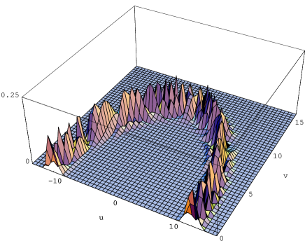
Figure 1: Left, plot of the $|\mbox{Re}\,\psi(u,v)|^{2}$ of the solution to the Wheeler-DeWitt Eq. (1) with 130 basis states used in the expansion of the solution. Right, $|\mbox{Re}\,\psi(u,v)|^{2}$ of this solution along the classical circular path [18] (i.e. along its crest .)

From the Figure it is obvious that the usage of explicit or implicit FDM would fail in this type of situations. Moreover for smaller classical path radii, although there will be less oscillations, the solutions that we attempted to find using FDM showed divergent behavior at large distances.

We are interested in solving problems which are generalizations of the one mentioned above. This gives us motivation to use a different numerical method to solve this type of problems. This method, which was first introduced by Galerkin, consists of first choosing a complete orthonormal set of eigenstates of a, preferably relevant, hermitian operator to be used as a suitable basis for our solution. For this numerical method we obviously can not choose the whole set of the complete basis, as these are usually infinite. Therefore we make the approximation of representing the solution by only a finite superposition of the basis functions. By substituting this approximate solution into the differential equation, a matrix equation is obtained. The expansion coefficients of these approximate solutions could be determined by eigenvalues and eigenfunctions of this matrix. This method has been called the Galerkin Method, and is a subset of the more general Spectral Method (SM) [9, 10, 11, 12]. Spectral methods fall into two broad categories. The interpolating , and the non interpolating method. The first category, which includes the Pseudospectral and the Spectral Element Methods, divides the configuration space into a set of grid points. Then one demands that the differential equation be satisfied exactly at a set of points known as the collocation or interpolation points. Presumably, as the residual function is forced to vanish at an increasingly larger number of discrete points, it will be smaller and smaller in the gaps between the collocation points. The non interpolating category includes the Lanczos tau-method and the Galerkin s method, mentioned above. The latter is the method that we apply and, in conformity with the usual nomenclature, we shall simply refer to it as the Spectral Method. The interesting characteristic of this method is that it is completely distinct from the usual spatial integration routines, such as FDM, which concentrate on spatial points. In SM the concentration is on the basis functions and we expect the final numerical solution to be approximately independent of the actual basis used. That is we expect the approximate solution to converge to the exact solution as the number of basis elements used increases. This point has been clearly demonstrated by Maday et. al. [13]. Moreover in this method, the refinement of the solution is accomplished by choosing a larger set of basis functions, rather than choosing more grid points, as in the numerical integration methods. We should note that we are implicitly assuming that the true solution is expandable in any complete orthonormal basis such as Fourier, Laguerre[14], Chebyshev[15], or Legendre[16] basis. However, this requirement is usually satisfied for cases of physical applications.

The paper is organized as follows: In section $2$ and $3$ we layout the implementation of this method using the quantum eigenfunctions for the simple harmonic oscillator, henceforth called the Oscillator basis, and the Fourier basis, respectively. In section $4$ we solve a particularly interesting example relevant to quantum cosmology by this method using both of the aforementioned basis functions. This problem is a generalization of the one represented in Eq. (1) and does not seem to have an exact solution, and we have not been able to solve this problem by any other numerical method that we tried. In section $5$ we discuss the accuracy of each of the cases, and make a comparison between the two. In section $6$ we discuss some general features of this method.

2 The Oscillator Basis

The general PDE equation that we want to solve is a hyperbolic one cast in the form,

$$H\psi(u,v)=\left\{-\frac{\partial^{2}}{\partial u^{2}}+\frac{\partial^{2}}{\partial v^{2}}+\omega_{1}^{2}u^{2}-\omega_{2}^{2}v^{2}+\hat{f}(u,v)\right\}\psi(u,v)=0,$$ (2)

where $\hat{f}(u,v)$ is an arbitrary operator of $u$ and $v$, but with derivatives less than two. Eq. (2) in general is not separable, however, any solution can be written as a superposition of the basis elements,

$$\psi_{m,n}(u,v)=\alpha_{m}(u)\beta_{n}(v),$$ (3)

where each of the sets $\{\alpha_{n}\}$ and $\{\beta_{m}\}$ is an orthonormal complete set. In this section we take both of them to be the Oscillator basis [17]. That is,

$$\alpha_{n}(u)=\left(\frac{\omega_{1}}{\pi}\right)^{1/4}\frac{H_{n}(\sqrt{\omega_{1}}u)}{\sqrt{2^{n}n!}}e^{-\omega_{1}u^{2}/2},$$ (4)

$$\beta_{n}(v)=\left(\frac{\omega_{2}}{\pi}\right)^{1/4}\frac{H_{n}(\sqrt{\omega_{2}}v)}{\sqrt{2^{n}n!}}e^{-\omega_{2}v^{2}/2},$$ (5)

where $H_{n}(x)$ denote the Hermite polynomials. In particular the set $\left\{\psi_{m,n}(u,v)\right\}$ is a complete orthonormal set which can be used to span the zero sector subspace of the Hilbert space of the hermitian operator $H$, as defined in Eq. (2). These basis elements are ${\cal L}^{2}$ measurable square integrable functions on $\bf R^{2}$ with an inner product defined in the usual way, so that the orthonormality, for example, takes the form,

$$\int\psi_{m,n}(u,v)\psi_{m^{\prime},n^{\prime}}(u,v)dudv=\delta_{m,m^{\prime}}\delta_{n,n^{\prime}}.$$

We can construct a general solution as follows,

$$\psi(u,v)=\sum_{m,n}A_{m,n}\alpha_{m}(u)\beta_{n}(v),$$ (6)

and can use the following expansion,

$$\hat{f}(u,v)\psi(u,v)=\sum_{m,n}B_{m,n}\alpha_{m}(u)\beta_{n}(v),$$ (7)

where $B_{m,n}$ are coefficients that can be determined once $\hat{f}(u,v)$ is specified. By substituting Eqs. (6,7) in Eq. (2), and using the differential equation of the Hermite polynomials we obtain,

$$\sum_{m,n}\Bigl{[}[(2m+1)\omega_{1}-(2n+1)\omega_{2}]A_{m,n}+B_{m,n}\Bigr{]}\alpha_{m}(u)\beta_{n}(v)=0.$$ (8)

Because of the linear independence of $\alpha_{m}(u)$s and $\beta_{n}(v)$s, every term in the summation must satisfy,

$$[(2m+1)\omega_{1}-(2n+1)\omega_{2}]A_{m,n}+B_{m,n}=0.$$ (9)

It only remains to determine the matrix $B$. By using Eqs. (6,7) we have,

$$\sum_{m,n}B_{m,n}\alpha_{m}(u)\beta_{n}(v)=\sum_{m,n}A_{m,n}\hat{f}(u,v)\alpha_{m}(u)\beta_{n}(v).$$ (10)

By multiply both sides of the above equation by $\alpha_{m^{\prime}}(u)\beta_{n^{\prime}}(v)$ and integrating over the full range of variables $u$ and $v$, and using orthonormality of the basis functions, one finds,

$$B_{m,n}=\sum_{m^{\prime},n^{\prime}}\left(\int_{-\infty}^{\infty}\int_{-\infty}^{\infty}\alpha_{m}(u)\beta_{n}(v)\hat{f}(u,v)\alpha_{m^{\prime}}(u)\beta_{n^{\prime}}(v)dudv\right)A_{m^{\prime},n^{\prime}}\equiv\sum_{m^{\prime},n^{\prime}}C_{m,n,m^{\prime},n^{\prime}}A_{m^{\prime},n^{\prime}}.$$ (11)

Therefore we can rewrite Eq. (9) as,

$$[(2m+1)\omega_{1}-(2n+1)\omega_{2}]A_{m,n}+\sum_{m^{\prime},n^{\prime}}C_{m,n,m^{\prime},n^{\prime}}\,\,A_{m^{\prime},n^{\prime}}=0.$$ (12)

It is obvious that the presence of the operator $\hat{f}(u,v)$ in Eq. (2), leads to nonzero coefficients $C_{m,n,m^{\prime},n^{\prime}}$ in Eq. (12), which in principle could couple all of the matrix elements of $A$. For the usual choices of $\hat{f}(u,v)$, e.g. the choice presented in [8]: $\hat{f}=\frac{9}{4}k(u^{2}-v^{2})^{1/3}$, the problem, to the best of our knowledge, is not analytically solvable. Therefore we have to resort to a numerical solution. In general the number of basis elements are at least countably infinite. The aforementioned coupling of terms in the main matrix Eq. (12) forces us to make the approximation of using a finite basis. It is easy to see that the more basis functions we include, the closer our solution will be to the exact one. We select the first $N$ basis functions in each direction, that is $m$ and $n$ run from $1$ to $N$. Then we replace the square matrix $A$ with a column vector $A^{\prime}$ with $N^{2}$ elements, so that any element of $A$ corresponds to one element of $A^{\prime}$. With this replacement, Eq(̇12) can be written as,

$$D\,A^{\prime}=0,$$ (13)

where $D$ is a square matrix with $N^{2}\times N^{2}$ elements which can be obtained from Eq. (12). Looked upon as an eigenvalue equation, i.e. $DA^{\prime}_{a}=aA^{\prime}_{a}$, the matrix $D$ has $N^{2}$ eigenvectors. However, for constructing the acceptable wavefunctions, i.e. the ones satisfying the WD Eq. (2), we only require eigenvectors which span the null space of the matrix $D$. That is, due to Eq. (12) we will have exactly $N$ null eigenvectors which will be linear combination of our original eigenfunctions introduced in Eq. (3). After finding these $N$ eigenvectors $A^{\prime i}$ ($i=1,2,3,...,N$), we can find the corresponding elements of the matrix $A$, $A_{m,n}^{i}$. Therefore the wavefunction can be expanded as,

$$\psi(u,v)=\sum_{i}\lambda^{i}\psi^{i}(u,v),$$ (14)

where $\psi^{i}(u,v)$ are the appropriate eigenfunctions for the problem (i.e. Eq. (2)),

$$\psi^{i}(u,v)=\sum_{m,n}A_{m,n}^{i}\alpha_{m}(u)\beta_{n}(v).$$ (15)

In Eq. (14) $\lambda^{i}$s are arbitrary complex constants to be determined by the initial conditions.

3 The Fourier Basis

As mentioned before, any complete orthonormal set can be used for this SM. In this section we use the Fourier series basis as a second example. That is, since we need to choose a finite subspace of a countably infinite basis, we restrict ourselves to a finite square region of sides $2L$. This means that we can expand the solution as,

$$\psi(u,v)=\sum_{i,j=1}^{2}\sum_{m,n}A_{m,n,i,j}\,\,\,g_{i}\left(\frac{m\pi u}{L}\right)\,\,\,g_{j}\left(\frac{n\pi v}{L}\right),$$ (16)

where,

$$\left\{\begin{array}[]{ll}g_{1}\left(\frac{m\pi u}{L}\right)=\sqrt{\frac{2}{R_{m}L}}\sin\left(\frac{m\pi u}{L}\right),&\\ g_{2}\left(\frac{m\pi u}{L}\right)=\sqrt{\frac{2}{R_{m}L}}\cos\left(\frac{m\pi u}{L}\right).&\\ \end{array}\right.\mbox{and}\,\,\,R_{m}=\left\{\begin{array}[]{ll}1,&m\neq 0\\ 2,&m=0\\ \end{array}\right.$$

That is in the Fourier basis we assume periodic boundary condition. By referring to the WD Eq. (2), we realize that in the Fourier basis it is appropriate to introduce $\hat{f}^{\prime}$ as,

$$\hat{f}^{\prime}(u,v)=f(u,v)+\omega_{1}^{2}u^{2}-\omega_{2}^{2}v^{2},$$ (17)

and, in analogy with Eq. (7), we can make the following expansion,

$$\hat{f}^{\prime}(u,v)\psi(u,v)=\sum_{i,j}\sum_{m,n}B^{\prime}_{m,n,i,j}\,\,\,g_{i}\left(\frac{m\pi u}{L}\right)\,\,\,g_{j}\left(\frac{n\pi v}{L}\right).$$ (18)

By following steps analogous to those of Eqs. (8-11) we obtain,

$$\left[\left(\frac{m\pi}{L}\right)^{2}-\left(\frac{n\pi}{L}\right)^{2}\right]A_{m,n,i,j}+B^{\prime}_{m,n,i,j}=0,$$ (19)

where

$$B^{\prime}_{m,n,i,j} = \sum_{m^{\prime},n^{\prime},i^{\prime},j^{\prime}}\left[\int\int_{-L}^{L}g_{i}\left(\frac{m\pi u}{L}\right)g_{j}\left(\frac{n\pi v}{L}\right)\hat{f}^{\prime}(u,v)g_{i^{\prime}}\left(\frac{m^{\prime}\pi u}{L}\right)g_{j^{\prime}}\left(\frac{n^{\prime}\pi v}{L}\right)dudv\right]A_{m^{\prime},n^{\prime},i^{\prime},j^{\prime}}$$ (20)

$$= \sum_{m^{\prime},n^{\prime},i^{\prime},j^{\prime}}C^{\prime}_{m,n,i,j,m^{\prime},n^{\prime},i^{\prime},j^{\prime}}\,\,A_{m^{\prime},n^{\prime},i^{\prime},j^{\prime}},$$

Therefore we can rewrite Eq. (19) as

$$\left[(m\pi)^{2}-(n\pi)^{2}\right]A_{m,n,i,j}+\sum_{m^{\prime},n^{\prime},i^{\prime},j^{\prime}}C^{\prime}_{m,n,i,j,m^{\prime},n^{\prime},i^{\prime},j^{\prime}}\,\,A_{m^{\prime},n^{\prime},i^{\prime},j^{\prime}}=0.$$ (21)

In this case, we select $4N^{2}$ basis functions. Using reasoning analogous to the previous case, for example by defining the column vector $A^{\prime}$ out of the matrix $A$, we transform Eq. (21) to

$$D^{\prime}\,A^{\prime}=0.$$ (22)

Where, as before, $D^{\prime}$ is a square matrix now with $(2N)^{2}\times(2N)^{2}$ elements which can be easily obtained from Eq. (21). After finding the $4N^{2}$ eigenvectors of $D^{\prime}$, we select the 2N ones with zero eigenvalue, i.e. $A^{\prime k}$ ($k=1,2,3,...,2N$). We can then find the corresponding elements of matrix $A$, $A^{k}_{m,n,i,j}$. Therefore, the wavefunction can be expanded as

$$\psi(u,v)=\sum_{k}\lambda^{k}\psi^{k}(u,v),$$ (23)

where, as before, $\psi^{k}(u,v)$ are the appropriate eigenfunctions for the problem (i.e. Eq. (2)),

$$\psi^{k}(u,v)=\sum_{m,n,i,j}A^{k}_{m,n,i,j}\,\,\,g_{i}\left(\frac{m\pi u}{L}\right)\,\,\,g_{j}\left(\frac{n\pi v}{L}\right).$$ (24)

Here $\lambda^{k}\,\,$s in Eq. (23) are again arbitrary complex constants to be determined by the initial conditions.

Now we apply this method to one of the examples stated above which happens to be relevant in quantum cosmology, and was our original motivation for using this method.

4 Application of the Spectral Method to a Specific Example

For a specific example, we consider a hyperbolic PDE which happens to be the Wheeler-DeWitt equation for the Robertson-Walker quantum cosmology with non-zero curvature,

$$\left\{-\frac{\partial^{2}}{\partial u^{2}}+\frac{\partial^{2}}{\partial v^{2}}+\omega^{2}_{1}u^{2}-\omega_{2}^{2}v^{2}+\frac{9}{4}k(u^{2}-v^{2})^{1/3}\right\}\psi(u,v)=0.$$ (25)

As mentioned before, the case $k=0$ is exactly solvable [8] and has a closed form solution in the Oscillator basis. We shall state these solutions here for illustrative purposes, especially for motivating the choice of initial conditions and comparison with the non-trivial cases, i.e $k\neq 0$, which shall be solved by this method next. In this case $f(u,v)=0$ in Eq. (2), so the matrix $B$ in Eq. (9) is also zero due to Eq. (7). Therefore, Eq. (9) reduces to,

$$\left[(2m+1)\omega_{1}-(2n+1)\omega_{2}\right]A_{m,n}=0.$$ (26)

This means $A_{m,n}=0$ for,

$$\omega_{2}\neq\frac{2m+1}{2n+1}\omega_{1}.$$ (27)

That is we have nontrivial solutions only for $\omega_{1}$ and $\omega_{2}$ being a rational multiple of each other. Choosing $\omega_{1}=\omega_{2}$ for simplicity, we have $n=m$ and the expansion of the wavefunction (Eq. (6)) reduces to,

$$\psi(u,v)=\sum_{m}A_{m}\alpha_{m}(u)\beta_{m}(v),$$ (28)

where $A_{m}\equiv A_{m,m}$ are complex expansion coefficients that can be determined by applying initial conditions (i.e. specifying $\psi(u,0)$ and $\frac{\partial\psi}{\partial v}|_{v=0}$). In references [8, 18] the authors considered the following initial condition on the wave function,

$$\psi(u,0)=\frac{1}{2\pi^{1/4}}\left(e^{-(x-\chi)^{2}/2}+e^{-(x+\chi)^{2}/2}\right).$$ (29)

We can decompose any initial wavefunction in the Oscillator basis. For the choice presented in Eq. (29) we have,

$$\psi(u,0)=\sum_{n}^{{}^{\prime}}c_{n}\alpha_{n}(u),\hskip 14.22636pt\mbox{where}\hskip 14.22636ptc_{n}=e^{-\frac{1}{4}|\chi|^{2}}\frac{\chi^{n}}{\sqrt{2^{n}n!}}\,,$$ (30)

and $\chi$ is an arbitrary complex number. The prime on the summation denotes the restriction that $n$ is even. These coefficients are same as those of the coherent states of a one dimensional simple harmonic oscillator. With this choice of coefficients we expect that a classical-quantum correspondence should be manifest. The canonical choice for initial slope is [8],

$$\left.\frac{\partial\psi}{\partial v}\right|_{v=0}=\sum_{n}\frac{c_{n}\alpha_{n}(u)H^{\prime}_{n}(0)}{\frac{(-1)^{(n/2)}n!}{(n/2)!}},$$ (31)

where $H_{n}$s are the Hermite polynomials and prime denotes differentiate respect to $v$. By choosing $\chi$ to be a real, the classical paths corresponding to these solutions can be shown to be circles with radii $\chi$. We have found that $35$ basis functions are sufficient for finding the solution to an accuracy of about $10^{-8}$ , when the classical radius of the wave packet ($\chi$) is less than $4$ (Fig. 2). As can be seen in the figure, and also for all the cases presented in [8], the classical-quantum correspondence is manifest. Note that the wave packet has compact support and in the oscillator basis, the truncation of the basis functions automatically restricts the solution to have this property. We only need to choose the configuration space domain to be large enough.

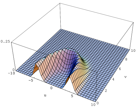
Figure 2: Oscillator Basis: Left, the absolute value squared of the wave packet $|\psi(u,v)|^{2}$ for $\chi=4$ and $N=35$, $k=0$. Right, the contour plot of the same figure with the classical path superimposed as the thick solid line.

At this point it seems to us that a brief mention of the relevant dynamical equations for the classical cosmology might be helpful, at least for completeness, especially in light of the fact that “classical-quantum correspondence” that we keep mentioning in this paper is particularly important in physics. Moreover, the non-linearity and the moving singular behavior of these equations would become apparent. These equations are (see, for example, [19]),

$$\ddot{u}+u+\frac{3k}{2}\frac{u}{(u^{2}-v^{2})^{2/3}}=0,$$ (32)

$$\ddot{v}+v+\frac{3k}{2}\frac{v}{(u^{2}-v^{2})^{2/3}}=0,$$ (33)

$$\dot{u}^{2}+u^{2}-\dot{v}^{2}-v^{2}+\frac{9}{4}k(u^{2}-v^{2})^{1/3}=0.$$ (34)

Here the $u$ and $v$ variables are functions of time. Equations (32) and (33) are the dynamical equations and, Eq. (34) is the zero energy constraint, from which the Wheeler-deWitt Eq. (25) arises. An appropriate initial conditions is the following,

$$u(0)=-\chi,\hskip 28.45274ptv(0)=0,\hskip 28.45274pt\dot{u}(0)=0,\hskip 28.45274pt\dot{v}(0)=\dot{v}_{0},$$ (35)

where $\chi$ can be treated as a free parameter and $\dot{v}_{0}$ is adjusted so that Eq. (34) is satisfied. With this choice of initial conditions the classical path would be, as mentioned before, exactly a circle in the $k=0$ case, as depicted in Fig. 2. In the general case of $\omega_{1}\neq\omega_{2}$, these solutions would give Lissajous figures.

For the case $k\neq 0$, the problem is not exactly solvable in quantum cosmology and we will use the SM to get an approximate solution. We have to mention that the corresponding equations for classical cosmology, Eqs. (32)-(34), are a set of non-linear, coupled ODEs with moving singularities which are not exactly solvable either. However, a general method for solving them has been presented in [20], and this is the method we shall use. Also a detailed explanation of the physical setting of the problem in the classical domain has been presented in [19]. On one hand, we need to choose a set of appropriate initial conditions for both the classical and quantum cases which would make their correspondence manifest when they are superimposed, as in Fig. 2 which was for the $k=0$ case. However, we should note that the values of $\dot{v}_{0}$ in the classical case depends on $k$. On the other hand, an appropriate choice for the initial conditions should be such that we could easily compare our results with the $k=0$ case. Therefore, here we choose the same initial conditions for the quantum cosmology Eqs. (30,31), and classical cosmology Eq. (35), as for the $k=0$ case. An alternative would be to choose appropriate initial canonical slope for the quantum cosmology case [21]. Having set the initial conditions, we proceed to solve the quantum cosmology problem for the case $k\neq 0$ with the Oscillator basis.

Both the classical and quantum solutions for the case $k=+1$ are shown in Fig. 3. We can see that the general behavior of this case is similar to the $k=0$ case. In particular, again we have a very good classical-quantum correspondence. However, although the extreme points of the solution do not change as compared to the $k=0$ case, the whole pattern is a little wider. Moreover, the solution ($|\psi|^{2}$) is not as smooth as $k=0$ case.

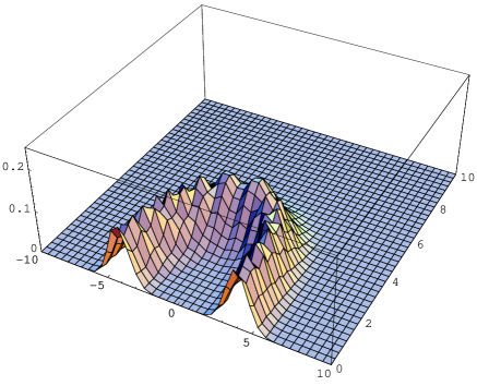
Figure 3: Oscillator Basis: Left, the absolute value squared of the wave packet $|\psi(u,v)|^{2}$ for $\chi=4$ and $N=35$, $k=+1$. Right, the contour plot of the same figure with the classical path superimposed as the thick solid line.

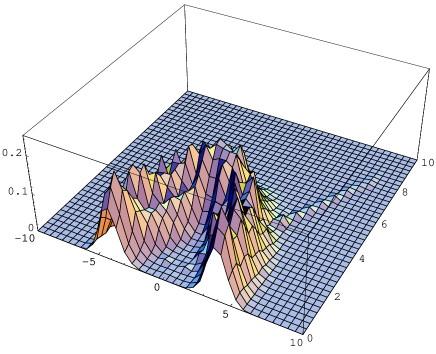
Figure 4: Oscillator Basis: Left, the absolute value squared of the wave packet $|\psi(u,v)|^{2}$ for $\chi=4$ and $N=35$, $k=-1$. Right, the contour plot of the same figure with the classical path superimposed as the thick solid line.

Both the classical and quantum solutions for the case $k=-1$ are shown in Fig. 4. We can see that the general behavior of this case is also similar to the $k=0$ case. In particular, again we have a very good classical-quantum correspondence. However, although the extreme points of the solution do not change as compared to the $k=0$ case, the whole pattern is a little narrower. Moreover, the solution ($|\psi|^{2}$) is not as smooth as $k=0$ case. More importantly, when $k=-1$ we encounter a new characteristic of the solution. Note that the $u^{2}-v^{2}$ term in Eq. (25) is usually dominant and causes stability of the solutions, for all $k$. However, the $\frac{9}{4}k(u^{2}-v^{2})^{(1/3)}$ term in that equation could cause instability near $u=\pm v$ lines, only in the case of $k<0$. However this is precisely where the dominant term vanishes. Therefore we do expect numerical instabilities along these two lines for this case. These instabilities can be seen in Fig. 4. However, due to numerical approximations made, the instabilities seem to be more pronounced along the line $u=v$ in our solution. We have not been able to the pinpoint the exact source of this numerical asymmetry in the instability.

It would be an interesting comparison to solve exactly the same problem in the Fourier basis. By using the procedure mentioned in section 3, and again choosing exactly $35$ basis functions for ease of comparison, we easily find the solutions for $k=0$, $k=1$ and $k=-1$, which are shown in Figs. (5-7), respectively.

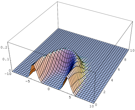
Figure 5: Fourier Basis: Left, the absolute value squared of the wave packet $|\psi(u,v)|^{2}$ for $\chi=4$ and $N=35$, $k=0$. Right, the contour plot of the same figure with the classical path superimposed as the thick solid line.

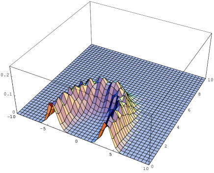
Figure 6: Fourier Basis: Left, the absolute value squared of the wave packet $|\psi(u,v)|^{2}$ for $\chi=4$ and $N=35$, $k=1$. Right, the contour plot of the same figure with the classical path superimposed as the thick solid line.

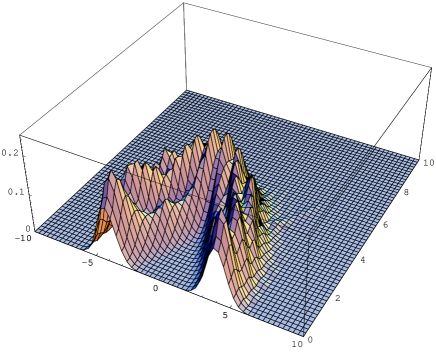
Figure 7: Fourier Basis: Left, the absolute value squared of the wave packet $|\psi(u,v)|^{2}$ for $\chi=4$ and $N=35$, $k=-1$. Right, the contour plot of the same figure with the classical path superimposed as the thick solid line.

5 Comparison of the Oscillator and Fourier Bases

Here, we compare the results of the Spectral Method using the two finite bases. To this end, we first discuss the errors of the solutions. In the case $k=0$ we have the exact solutions as an infinite series. For small radii, e.g.  $\chi=4$, the difference between the exact solution and a series solution with $120$ oscillator terms is absolutely negligible. Therefore, we can safely substitute this finite series for the exact one. For computing errors, we divide the $2D$ base domain into $M^{2}$ grid points. Then, we average the square of the absolute value of the difference of the exact solution with that obtained by the $35$ Fourier or oscillator basis functions on the grid points:

$$\delta^{2}_{k=0}=\frac{\sum_{i,j}^{M}|\psi_{35}(i,j)-\psi_{120}(i,j)|^{2}}{\sum_{i,j}^{M}|\psi_{120}(i,j)|^{2}}.$$ (36)

In the case $k\neq 0$ the problem is not exactly solvable, so for comparison purposes we define a measure for the error as the average square of the absolute value of the difference of the solutions with, for example, $35$ and $30$ basis functions. That is,

$$\delta^{2}_{k\neq 0}=\frac{\sum_{i,j}^{M}|\psi_{35}(i,j)-\psi_{30}(i,j)|^{2}}{\sum_{i,j}^{M}|\psi_{35}(i,j)|^{2}}.$$ (37)

	$\delta_{Fourier}$	$\delta_{oscillator}$
$k=0$	$6.70875\times 10^{-2}$	$4.16459\times 10^{-7}$
$k=+1$	$4.01423\times 10^{-3}$	$3.84836\times 10^{-2}$
$k=-1$	$2.83746\times 10^{-3}$	$3.64503\times 10^{-2}$

Table I. Errors for the Oscillator and Fourier basis

From Table I we can conclude that the oscillator basis is more appropriate than Fourier basis for the case $k=0$. It seems that this is only due to the fact that the Oscillator basis is the exact solution of the problem in this case. However, the Fourier basis is more appropriate for the case $k\neq 0$. The main reason for this seems to us to be the fact that the solutions have compact support, so we have an extra parameter that we can adjust (the size of spatial domain (2L)) and this yields better results. In fact one can use this freedom to set up an optimization procedure [22].

6 Discussion

Here we have exhibited the implementation of the SM (Galerkin) for solving hyperbolic PDEs. We use finite basis of Oscillator or Fourier eigenfunctions, for example, and show that in some cases where the popular numerical methods such as FDM or FEM fail, this method gives reasonable results very easily. The requirement that the solution should be expandable in a complete orthonormal basis is crucial. However, certain bases might be more appropriate for a given problem. For example, if the wave packets of previous section was not damped strongly in $u$ and $v$ directions, choosing oscillator basis might not have been as appropriate. We have found, much to our surprise, that the main source of error is the numerical integrations, as compared to varying the number of basis elements. This arise due to the fact that in order to find the coefficients $C(m,n,m^{\prime},n^{\prime})$, we need to calculate $N^{4}$ two fold integrations, where $N$ denotes the number of basis elements. This is the most time consuming part of the procedure. Using programs with refined integration routines such as Mathematica would have consumed too much time even at their default levels. So we used the simple trapezoid integration technique using Fortran, and this severely limited our accuracy when we refrained from refining our mesh excessively to avoid spending too much time. However, calculations of $C(m,n,m^{\prime},n^{\prime})$s can be parallelized because these coefficients are independent. In some cases we can calculate some of the integrals analytically (e.g.  the values of $C^{\prime}_{m,n,i,j,m^{\prime},n^{\prime},i^{\prime},j^{\prime}}$ in Eq. (20) when $k=0$), which decreases the computation time. The memory consuming part of the procedure is solving the matrix equation (Eq. (13)) and this increases proportional to $N^{4}$.

AcknowledgementThis research has been supported by the office of research of Shahid Beheshti University under Grant No. 500/3787.

References

- [1] Richard L. Burden and J. Douglas Faires. Numerical Analysis. Brooks/Cole, 7 edition, (2001).
- [2] J. M. Ortega and W. G. Poole, An Introduction to Numerical Methods for Differential Equations Academic Press, New York (1981).
- [3] MIG. Bloor and M.J. Wilson, Representing PDE surfaces m terms of B-splines, Comput.-Aided Des. Vol22 (1990), pp 324-331.
- [4] Chen. Zhangxin, Finite Element Methods And Their Applications, Zhangxin Chen, Springer, (2005).
- [5] D K Brown, Introduction to the Finite Element Method Using Basic Programs, Spon Press (UK), (1998).
- [6] W.H. Press, S.A. Teukolsky, W.T. Vetterling, and B.P. Flannery. Numerical Recipes in Fortran - The Art of Scientic Computing. Cambridge University Press, 2nd edition, 1992.
- [7] B. S. DeWitt, Phys. Rev. 160 (1967) 1113.
- [8] S. S. Gousheh and H. R. Sepangi, Phys.Lett. A272 (2000), 304.
- [9] J. P. Boyd, Chebyshev & Fourier Spectral Methods, Springer-Verlag, BerlinHeidelberg, (1989).
- [10] D. Gottleib and S. Ortega, Numerical analysis of spectral methods: theory and applications, SIAM, Philadelphia (1977).
- [11] C. Canuto, M. Y. Hussaini, A. Quateroni and T. Zang, Spectral Methods in Fluid Dynamics Springer, Berlin (1988).
- [12] C. Bernardi, Y. Maday, Spectral methods, in: P.G. Ciarlet, J.L. Lions (Eds.), Handbook of Numerical Analysis V, Elsevier Sciences, North-Holland, The Netherlands, (1999).
- [13] Y. Maday, A.T. Patera and G. Turinici, C. R. Acad. Sci. Paris Sér. I 335 (2002), 289.
- [14] Y. Maday, B. Pernaud-Thomas, and H. Vandeven, Rech. Aerospat., 6 (1985) 353.
- [15] C. Bernardi, C. Canuto and Y. Maday , SIAM J. Numer. Anal. 25 (1988), 1237.
- [16] Y. Maday, S.M. Ould Kaper, E. Tadmor, SIAM J. Numer. Anal. 30 (1993) 321.
- [17] D. Funaro and O. Kavian , Math. Comp. 57 (1990), 597.
- [18] C. Kiefer , Nucl. Phys. B341 (1990) 273.
- [19] K. Ghafoori-Tabrizi, S. S. Gousheh and H. R. Sepangi, Int. J. Mod. Phys. A 15 (2000), 1521.
- [20] S. S. Gousheh and H. R. Sepangi, K. Ghafoori-Tabrizi, Computer Physics Communications, 149 (2003), 135.
- [21] H. R. Sepangi, S. S. Gousheh, P. Pedram, and M. Mirzaei, gr-qc/0701035.
- [22] P. Pedram, M. Mirzaei and S. S. Gousheh, math-ph/0611008.