Development of Fractal Geometry in a 1+1 Dimensional Universe

Abstract

Observations of galaxies over large distances reveal the possibility of a fractal distribution of their positions. The source of fractal behavior is the lack of a length scale in the two body gravitational interaction. However, even with new, larger, sample sizes from recent surveys, it is difficult to extract information concerning fractal properties with confidence. Similarly, simulations with a billion particles only provide a thousand particles per dimension, far too small for accurate conclusions. With one dimensional models these limitations can be overcome by carrying out simulations with on the order of a quarter of a million particles without compromising the computation of the gravitational force. Here the multifractal properties of a group of these models that incorporate different features of the dynamical equations governing the evolution of a matter dominated universe are compared. The results share important similarities with galaxy observations, such as hierarchical clustering and apparent bifractal geometry. They also provide insights concerning possible constraints on length and time scales for fractal structure. They clearly demonstrate that fractal geometry evolves in the $\mu$ (position, velocity) space. The observed properties are simply a shadow (projection) of higher dimensional structure.

I Introduction

Starting with the work of Vaucoulours,de Vaucouleurs (1970) questions have been posed about the geometric properties of the distribution of matter in the universe. Necessary for all modern cosmologies are the assumptions of homogeneity and isotropy of the mass distribution on large length scales.Peebles (1993) However, observations have shown the existence of very large structures such as super-clusters and voids.Pecker and Narlikar (2006) Moreover, as technology has advanced, so has the length scale of the largest observed structures. (For a recent review see Jones et. al.Jones et al. (2004).) It was proposed by Mandelbrot,Mandelbrot (1982) based on work of Peebles,Peebles (1993) that the matter distribution in the universe is fractal. Support for this conjecture came primarily from the computation of the pair correlation function for the positions of galaxies, as well as from direct observation. The fact that the correlation function was well represented by a power law in the intergalactic distance seemed to support the fractal conjecture. In fact, in the past it has been argued by Pietronero and colleagues that the universe may even be fractal on all scales.Jones et al. (2004)Labini et al. (1998) Of course, if this were true it would wreak havoc with the conclusions of cosmological theory.

McCauley has looked at this issue from a few different perspectives. He points out that since the power law behavior of the correlation function is only quantitatively correct over a finite length scale, the universe could not be a simple (mono) fractal.McCauley (2002) Then the logical next question is whether or not the matter distribution is multifractal. By considering counts in cells, Bailin and Schaeffer hypothesized some time ago that the distribution of matter is approximately bifractal, i.e. a superposition of fractals with two distinct scaling laws.Balian and Schaeffer (1989) McCauley has also addressed the possibility of inhomogeneity. Working with Martin Kerscher, he investigated whether the universe has multifractal geometry. His approach was to examine the point-wise dimension Ott (2002) by looking for local scaling of the density around individual galaxies in two catalogues. Their conclusion was that, even if local scaling were present, there are large fluctuations in the scaling law. Moreover, the sample sizes were not sufficient to be able to extract good local scaling exponents. Although larger galaxy catalogues have become available since their analysis, they do not meet the restrictive criteria of sufficient size, as well as uniform extension in all directions, necessary to measure local dimensions. Jones et al. (2004) Their final conclusion was that, while the geometry of the observed universe is certainly not monofractal, it was not possible to irrefutably conclude whether it is multifractal, or whether the assumptions of homogeneity and isotropy prevail at large length scales.McCauley (2002)

If current observations aren’t able to let us determine the geometry of the universe, then we need to turn to theory and simulation. For the most part, we are concerned with the evolution of matter after the period of recombination. Consequently the Hubble expansion has slowed down sufficiently that Newtonian dynamics is applicable, at least within a finite region of space.chan Hwang and Noh (2006) A number of theoretical approaches to the computation of fractal dimensions have been investigated. Each of them is predicated on some external assumption which is not yet verified. For example, de Vega et. al. assume that the universe is close to a thermodynamic critical point de Vega and Sanchez (2000) , while Grujic explores a field theory where vacuum energy predominates over inert matter, and the latter is assumed to have a fractal structuring Grujic (2005). An examination of the recent literature reveals that theory has not converged on a compelling and uniformly accepted theory of fractal structure in the universe.

In the last few decades dynamical N-body simulation of cold dark matter CDM has experienced rapid advances due to improvements in both algorithms and technology.Bagla (2005); Bertschinger (1998) It is now possible to carry out gravitational N-body simulations with upwards of $10^{9}$ point mass particles. However, in order to employ simulation methods for systems evolving over cosmological time, it is necessary to compromise the representation of the gravitational interaction over both long and short length scales. For example, tree methods are frequently employed for large separations, typically the gravitational field is computed from a grid, and a short range cut-off is employed to control the singularity in the Newtonian pair potential.Bagla (2005); Bertschinger (1998) Unfortunately, even if the simulations were perfect, a system of even $10^{9}$ particles provides only $10^{3}$ particles per dimension and would thus be insufficient to investigate the fractal geometry with confidence.

As a logical consequence of these difficulties it was natural that physicists would look to lower dimensional models for insight. Although this sacrifices the correct dynamics, it provides an arena where accurate computations with large numbers of particles can be carried out for significant cosmological time. It is hoped that insights gained from making this trade-off are beneficial. In one dimension, Newtonian gravity corresponds to a system of infinitesimally thin, parallel, mass sheets of infinite spatial extent. Since there is no curvature in a 1+1 dimensional gravitational system, we cannot expect to obtain equations of motion directly from general relativity. Mann and Chak (2002) Then a question arises concerning the inclusion of the Hubble flow into the dynamical formulation. This has been addressed in two ways: In the earliest, carried out by Rouet and Feix, the scale function was directly inserted into the one dimensional dynamics.Rouet et al. (1990, 1991) Alternatively, starting with the usual three dimensional equations of motion and embedding a stratified mass distribution, Fanelli and Aurell obtained a similar set of coupled differential equations for the evolution of the system in phase space.Fanelli and Aurell (2002) While the approaches are different, from the standpoint of mathematics the two models are very similar and differ only in the values of a single fixed parameter, the effective friction constant. Following Fanelli,Fanelli and Aurell (2002) we refer to the former as the RF model and the latter as the Quintic, or Q, model.

By introducing scaling in both position and time, in each model autonomous equations of motion are obtained in the comoving frame. In addition to the contribution for the gravitational field, there is now a background term, corresponding to a constant negative mass distribution, and a linear friction term. By eliminating the friction term a Hamiltonian version can also be constructed. At least three other one dimensional models have also been investigated, one consisting of Newtonian mass sheets which stick together whenever they cross,Kofman et al. (1992) one evolved by directly integrating the Zeldovich equations,Shandarin and Zeldovich (1989); Tatekawa and Maeda (2001) and the continuous system satisfying Burger’s equation Gurbatov et al. (1997). In addition, fractal behavior has been studied in the autonomous one dimensional system where there is no background Hubble flow.Koyama and Konishi (2001, 2002)

In dynamical simulations, both the RF and Quintic model clearly manifest the development of hierarchical clustering in both configuration and $\mu$ space (the projection of the phase space on the position-velocity plane). In common with the observation of galaxy positions, as time evolves both dense clusters and relatively empty regions (voids) develop. In their seminal work, by computing the box counting dimension for the RF model, Rouet and Feix were able to directly demonstrate the formation of fractal structure.Rouet et al. (1990, 1991) They found a value of about 0.6 for the box counting dimension of the well evolved mass points in the configuration space, indicating the formation of a robust fractal geometry. In a later work, Miller and Rouet investigated the generalized dimension of the RF model.B.N.Miller and Rouet (2002) In common with the analysis of galaxy observations by Bailin and Schaeffer Balian and Schaeffer (1989) they found evidence for bi-fractal geometry. Although they did not compute actual dimensions, later Fanelli et. al. also found a suggestion of bi-fractal behavior in the model without friction Aurell et al. (2003). It is then not surprising that the autonomous, isolated, gravitational system which does not incorporate the Hubble flow also manifests fractal behavior for short times as long as the virial ratio realized by the initial conditions is very small.Koyama and Konishi (2001, 2002) In addition, in the one dimensional model of turbulence governed by Burger’s equation, the formation of shocks has the appearance of density singularities that are similar to the clusters found in the RF and Quintic model. A type of bi-fractal geometry has also been demonstrated for this system.Gurbatov et al. (1997)

Below we present the results of our recent investigation of multifractal properties of the Quintic model and the model without friction. In section II we will first describe the systems. Then we will give a straightforward derivation of the equations of motion and explain how they differ from the other models mentioned above. In section III we will explain how the simulations were carried out and describe their qualitative features. In section IV we define the generalized dimension and other fractal measures and present our approach for computing them. In section V we will present the results of the multifractal analysis. Finally conclusions will be presented in section VI.

II Description of the System

We consider a one dimensional gravitational system (OGS) of $N$ parallel, infinitesimally thin, mass sheets each with mass per unit area $m$ . The sheets are constrained to move perpendicular to their surface. Therefore we can construct a Cartesian axis $x$ perpendicular to the $N$ sheets. We imagine that the sheets are labeled by $j=1,...,N$. From its intersection with the $x$-axis, each sheet can be assigned the coordinate $x_{j}$ and the corresponding velocity $v_{j}$. From Gauss’ law, the force on each sheet is a constant proportional to the net difference between the total "mass" (really surface density) to its right and left. The equations of motion are

$$\frac{dx_{i}}{dt}=v_{i},\quad\frac{dv_{i}}{dt}=E_{i}=2\pi mG[N_{R,i}-N_{L,i}]$$ (1)

where $E_{i}$ is the gravitational field experienced by the i^th particle and $N_{R,i}$ ($N_{L,i}$) is the number of particles (sheets) to its right (left) . Because the acceleration of each particle is constant between crossings, the equations of motion can be integrated exactly. Therefore it is not necessary to use numerical integration to follow the trajectory in phase space. As a consequence it was possible to study the system dynamics on the earliest computers and it can be considered the gravitational analogue of the Fermi-Pasta-Ulam system.Weissert (1997) It was first employed by Lecar and Cohen to investigate the relaxation of an $N$ body gravitational system.Cohen and Lecar (1968) Although it was first thought that the $N$ body system would reach equilibrium with a relaxation time proportional to $N^{2}$ ,Hohl (1967) this was not born out by simulations.Wright et al. (1982) Partially because of its reluctance to reach equilibrium, both single and two component versions of the system have been studied exhaustively in recent years.Yawn and Miller (1997a, b)Posh et al. (1993)Milanovic et al. (1998)Milanovic et al. (2006)Rouet and Feix (1999) Most recently it has been demonstrated that, for short times and special initial conditions, the system evolution can be modeled by an exactly integrable system.B.Miller et al. (2005)

To construct and explore a cosmological version of the OGS we introduce the scale factor $A(t)$ for a matter dominated universe.Peebles (1993) Moreover, as discussed in the introduction, we are interested in the development of density fluctuations following the time of recombination so that electromagnetic forces can be ignored. For that, and later, epochs, the Hubble expansion has slowed sufficiently that Newtonian dynamics provides an adequate representation of the motion in a finite region.chan Hwang and Noh (2006) Then, in a $3+1$ dimensional universe, the Newtonian equations governing a mass point are simply

$$\frac{d\mathbf{r}}{dt}=\mathbf{v,\qquad}\frac{d\mathbf{v}}{dt}=\mathbf{E}_{g}\mathbf{(r,}t\mathbf{)}$$ (2)

where, here, $\mathbf{E}_{g}\mathbf{(r,}t\mathbf{)\ }$is the gravitational field. We wish to follow the motion in a frame of reference where the average density remains constant, i.e. the co-moving frame. Therefore we transform to a new space coordinate which scales the distance according to $A(t)$. Writing $\mathbf{r}=A(t)\mathbf{x}$ we obtain

$$\frac{d^{2}\mathbf{x}}{dt^{2}}+\frac{2}{A}\frac{dA}{dt}\frac{d\mathbf{x}}{dt}+\frac{1}{A}\frac{d^{2}A}{dt^{2}}\mathbf{x=}\frac{1}{A^{3}}\mathbf{E}_{g}(\mathbf{x},t)$$ (3)

where, in the above we have taken advantage of the inverse square dependence of the gravitational field to write $\mathbf{E}_{g}(\mathbf{x},t)=\frac{1}{A^{2}}\mathbf{E}_{g}\mathbf{(r},t)$ where the functional dependence is preserved. In a matter dominated (Einstein deSitter) universe we find that

$$A(t)=\left(\frac{t}{t_{0}}\right)^{\frac{2}{3}},\qquad\rho_{b}(t)=\left(6\pi Gt^{2}\right)^{-1}$$ (4)

where $t_{0}$ is some arbitrary initial time corresponding, say, to the epoch of recombination, $G$ is the universal gravitational constant, and $\rho_{b}(t)$ is the average, uniform, density frequently referred to as the background density. These results can be obtained directly from Eq.3 by noting that if the density is uniform, so that all matter is moving with the Hubble flow, the first two terms in Eq.3 vanish whereas the third term (times $A$) must be equated to the gravitational field resulting from the uniformly distributed mass contained within a sphere of radius $A\left|\mathbf{x}\right|$. Then the third term of Eq.3 is simply the contribution arising by subtracting the field due to the background density from the sphere.Peebles (1993) Noting that $A^{3}\rho_{b}(t)=\rho_{b}(t_{0})$ forces the result. Alternatively, also for the case of uniform density, taking the divergence of each side of Eq. 3 and asserting the Poisson equation forces the same result. Thus the Friedman scaling is consistent with the coupling of a uniform Hubble flow with Newtonian dynamics.Peebles (1993)

For computational purposes it is useful to obtain autonomous equations of motion which do not depend explicitly on the time. This can be effectively accomplished Rouet et al. (1990, 1991) by transforming the time coordinate according to

$$dt=B(t)d\tau,\qquad B(t)=\frac{t}{t_{0}}$$ (5)

yielding the autonomous equations

$$\frac{d^{2}\mathbf{x}}{d\tau^{2}}+\frac{1}{3t_{0}}\frac{d\mathbf{x}}{d\tau}-\frac{2}{9t_{0}^{2}}\mathbf{x=E}_{g}(\mathbf{x}).$$ (6)

For the Newtonian dynamics considered here it is necessary to confine our attention to a bounded region of space, $\Omega$. It is customary to choose a cube for $\Omega$ and assume periodic boundary conditions . Thus our equations correspond to a dissipative dynamical system in the comoving frame with friction constant $1/3t_{0}$ and with forces arising from fluctuations in the local density with respect to a uniform background.

For the special case of a stratified mass distribution the local density at time $t$ is given by

$$\rho(x,t)=\sum m_{j}(t)\delta(x-x_{j})$$ (7)

where $m_{j}(t)$ is the mass per unit area of the $j^{th}$ sheet and, from symmetry, the gravitational field only has a component in the $x$ direction. Then, for the special case of equal masses $m_{j}(t)=m(t)$, the correct form of the gravitational field occurring on the right hand side of Eq 6 at the location of particle $i$ is then

$$E_{g}(x_{i})=2\pi m(t_{0})G[N_{R,i}-N_{L,i}]$$ (8)

since we already implicitly accounted for the fact that $m_{j}(t)=m(t_{0})/A^{2}$ in Eq.6. The equations are further simplified by establishing the connection between $m(t_{0})$ and the background density at the initial time, $\rho_{b}(t_{0}).$ Let us assume that we have $2N$ particles (sheets) confined within a slab with width $2L$, i.e. $-2L<x<2L$. Then

$$\rho_{b}(t_{o})=\left(6\pi Gt_{o}^{2}\right)^{-1}=\left(\frac{N}{L}\right)m(t_{0}),$$ (9)

we may express the field by

$$E_{g}(x_{i})=2\pi m(t_{0})G[N_{R,i}-N_{L,i}]=\frac{2}{3t_{0}^{2}}\left(\frac{L}{N}\right)[N_{R,i}-N_{L,i}],$$ (10)

and the equations of motion for a particle in the system now read

$$\frac{d^{2}x_{i}}{d\tau^{2}}+\frac{1}{3t_{0}}\frac{dx_{i}}{d\tau}-\frac{2}{9t_{0}^{2}}x_{i}\mathbf{=}\frac{2}{3t_{0}^{2}}\left(\frac{L}{N}\right)[N_{R,i}-N_{L,i}].$$ (11)

It is convenient to refer to Jeans theory for the final choice of units of time and length Binney and Tremaine (1987)

$$T_{j}=\omega_{j}^{-1}=(4\pi G\rho)^{-1/2}=\sqrt{\frac{3}{2}}t_{o}$$

$$\quad\lambda_{j}=\lambda_{j}=v_{T}/\omega_{j}\sqrt{3\sigma_{v}^{2}/\omega_{j}^{2}}=\frac{3}{\sqrt{2}}\sigma_{v}t_{o},$$ (12)

where $\sigma_{v}^{2}$ is the variance of the velocity at the initial time, $v_{T}=\sigma_{v}=a/\sqrt{3}$ is the thermal velocity, and $a$ is the maximal absolute velocity value given to a particle when the initial distribution of velocities is uniform on $[-a,$$a$]. Then, with the further requirement that $L=n\lambda_{j},\quad 0<n<N,$ in these units our equations are

$$\frac{d^{2}x_{i}}{d\tau^{2}}+\frac{1}{\sqrt{6}}\frac{dx_{i}}{d\tau}-\frac{1}{3}x_{i}\mathbf{=}\left(\frac{n}{N}\right)[N_{R,i}-N_{L,i}].$$ (13)

There is still a final issue that we have to address. If we assume for the moment that the sheets are uniformly distributed and moving with the Hubble flow, then the first two terms above are zero. Unfortunately, if we take the average over each remaining term, we find that they differ by a factor of three. This seeming discrepancy arises because we started with spherical symmetry about an arbitrary point for the Hubble flow and are now imposing axial symmetry. If we imagine that we are in a local region with a stratified geometry, the symmetry is different and this has to be reflected in the background term. This apparent discrepancy can be rectified by multiplying the term in $x_{i}$ by three. Our final equations of evolution are then

$$\frac{d^{2}x_{i}}{d\tau^{2}}+\frac{1}{\sqrt{6}}\frac{dx_{i}}{d\tau}-x_{i}\mathbf{=}\left(\frac{n}{N}\right)[N_{R,i}-N_{L,i}].$$ (14)

The description is completed by assuming that the system satisfies periodic boundary conditions on the interval $2L$, i.e. when a particle leaves the primitive cell defined by $-2L<x<2L$ on the right, it re-enters at the left hand boundary with the identical velocity. Note that, in computing the field, we do not attempt to include contributions from the images of $x_{i}$ outside of the primitive cell.

Finally, we mention that the RF model is obtained from the reverse sequence where one first restricts the geometry to 1+1 dimensions and then introduces the transformation to the comoving frame. In this approach it is not necessary to make the adjustment in the coefficient of $x_{i}$ as we did here. This is quickly seen by noting that the divergence of $\mathbf{x}$ is three times greater than the divergence of $x\hat{x}$ which one would obtain by directly starting with the one dimensional model. However, in the RF model, the coefficient of the first derivative term (the friction constant) is $1/\sqrt{2}$ instead of $1/\sqrt{6}$. This simply illustrates that, since there is no curvature in a 1+1 dimensional universe, there is a degree of arbitrariness in choosing the final model. It cannot be obtained solely from General Relativity. For a discussion of this point see Mann et. al. . Mann and Chak (2002) A Hamiltonian version can also be considered by setting the friction constant to zero. In their earlier work, using the linearized Vlasov-Poisson equations, Rouet and Feix carried out a stability analysis of the model without friction. They determined that the system followed the expected behavior, i.e. when the system size is greater than the Jean’s length, instability occurs and clustering becomes possible.Rouet et al. (1990, 1991) We mention that, when the friction term is not present, both the Q and RF models are identical so, with the assumption that the friction term won’t have a large influence on short time, linear, stability, the analysis of the Hamiltonian version applies equally to each version.

The Vlasov-Poisson limit for the system is obtained by letting $N\rightarrow\infty$ and $m\rightarrow 0$ while constraining the density and energy (at a given time). Then, in the comoving frame, the system is represented by a fluid in the $\mu$ space. Let $f(x,v;t)$ represent the normalized distribution of mass in the $(x,v)$ phase plane at time $t$. From mass conservation, $f$ satisfies the continuity equation

$$\frac{\partial f}{\partial t}+v\frac{\partial f}{\partial x}+\frac{\partial af}{\partial v}=0,\quad a=-\gamma v-\frac{\partial\phi_{T}(x)}{\partial x}$$ (15)

which can also be derived using the identical scaling as aboveS. In Eq. (15), $a(x,v)$ is the local acceleration and $\phi_{T}$ is the potential function induced by the total density, including the effective negative background density, $-\rho_{b}$. Note that both $a(x,v)$ and $\phi_{T}$ are linear functionals of $f(x,v;t)$. Coupling Eq. (15) with the Poisson equation yields the complete Vlasov-Poisson system governing the evolution of $f(x,v;t)$. Depending on the final choice of the friction constant, $\gamma$, the continuum limit of either the Quintic or RF model can be represented by Eq.15. Note that an exact solution is

$$f(x,v,t)=\frac{|\rho_{b}|}{\sqrt{2\pi\sigma^{2}}}\exp{-\frac{v^{2}}{2\sigma^{2}}},\quad\sigma(t)=\sigma_{0}\exp{-\gamma t}$$ (16)

Using dynamical simulation, we will see that it is extremely unstable when the system size exceeds the Jeans’ length at the initial time.

Useful information can be had without constructing an explicit solution. For example, we quickly find that the system energy decreases at a rate proportional to the kinetic energy. The Tsallis entropy is defined by

$$S_{q}=\frac{1-\int{f^{q}dxdv}}{q-1},\quad\int\int{\ fdxdv}=1$$ (17)

In the limit $q\rightarrow 1$, $S_{q}$ reduces to the usual Gibbs entropy, $S_{1}=-\int{\int{f\ln{f}dx}dv}$. By asserting the Vlasov-Poisson evolution, we find that the Bolztmann-Gibbs entropy, $S_{1}$, decreases at the constant rate $-2\gamma$ while, for $q>1$, $S_{q}$ decreases exponentially in time. This tells us that the mass is being concentrated in regions of decreasing area of the phase plane, suggesting the development of structure. These properties are immediately evident for the trivial solution given above. By imposing a Euclidean metric in the phase plane, we can also investigate local properties such as the directions of maximum stretching and compression, as well as the local vorticity. We easily find that the rate of separation between two nearby points is a maximum in the direction given by

$$\tan(2\theta)=(1+\rho+\rho_{b})/\gamma,$$ (18)

where $\theta$ defines the angle with the coordinate axis in the $\mu$ space. Thus, in regions of low density, we expect to see lines of mass being stretched with constant positive slope in the phase plane. We will see below that this prediction is accurately born out by simulations.

III Simulations

An attraction of these one-dimensional gravitational systems is their ease of simulation. In both the autonomous (purely Newtonian without expansion) and RF models it is possible to integrate the motion of the individual particles between crossings analytically. Then the temporal evolution of the system can be obtained by following the successive crossings of the individual, adjacent, particle trajectories. This is true as well for the Q model. If we let $y_{i}=x_{i+1}-x_{i}$, where we have ordered the particle labels from left to right, then we find that the differential equation for each $y_{i}$ is the same, namely

$$\frac{d^{2}y_{i}}{d\tau^{2}}+\frac{1}{\sqrt{6}}\frac{dy_{i}}{d\tau}-y_{i}\mathbf{=-}\frac{2n}{N}.$$ (19)

The general solution of the homogenious version of E. 19 is a sum of exponentials. By including the particular solution of the inhomogenius equation (simply a constant) we obtain a fifth order algebraic equation in $u=\exp(\tau/\sqrt{6})$. Hence the name Q, or Quintic, model. These can be solved numerically in terms of the initial conditions by analytically bounding the roots and employing the Newton-Raphson method.Press et al. (1992) (Note that for the RF model a cubic equation is obtained.) A sophisticated, event driven, algorithm was designed to execute the simulations. Two important features of the algorithm are that it only updates the positions and velocities of a pair of particles when they actually cross, and it maintains the correct ordering of each particle’s position on the line. Using this algorithm we were able to carry out runs for significant cosmological time with large numbers of particles.

Typical numerical simulations were carried out for systems with up to $N=2^{18}$ particles. Initial conditions were chosen by equally spacing the particles on the line and randomly choosing their velocities from a uniform distribution within a fixed interval. For historical reasons we call this a waterbag. Other initial conditions, such as Normally distributed velocities, as well as a Brownian motion representation, which more closely imitates a cosmological setting, were also investigated. The simulations were carried forward for approximately fifteen dimensionless time units.

In Fig. 1 we present a visualization of a typical run with $2^{17}$particles. The system consists of the Q model with an initial waterbag distribution in the $\mu$ space. Initially the velocity spread is (-12.5, 12.5) in the dimensionless units employed here and the system contains approximately 16,000 Jeans’ lengths. In the left column we present a histogram of the particles positions at increasing time frames, while on the right we display the corresponding particle locations in $\mu$ (position, velocity) space. It is clear from the panels that hierarchical clustering is occurring, i.e. small clusters are joining together to form larger ones, so the clustering mechanism is “bottoms up”Peebles (1993). The first clusters are roughly the size of a Jean’s length and seem to appear at about $\tau=6$ and there are many while by $\tau=14$ there are on the order of 30 clusters. In the $\mu$ space we observe that between the clusters matter is distributed along linear paths. As time progresses the size of the linear segments increases. The behavior of these under-dense regions is governed by the stretching in $\mu$ space predicted by Vlasov theory explained above (see before Eq.(18)). The slopes of the segments are the same and in quantitative agreement with Eq. (18). Qualitatively similar histories are obtained for the RF model and the model without friction (see below), as well as for the different boundary conditions mentioned above. However, there are some subtle differences. In Fig. 2 we zoom in and show a sequence of magnified inserts from the $\mu$space at time T=14. The hierarchical structure observed in these models suggests the existence of a fractal structure, but careful analysis is required to determine if this is correct. Simulations have also been performed where the system size is less than the Jean’s length. The results support the standard stability analysis in that hierarchical clustering is not observed for these initial conditions.

Historically, power law behavior in the density-density correlation funtion has been taken as the most important signature of self similar behavior of the distribution of galaxy positions.Jones et al. (2004) In Figure 3 we provide a log-log plot of the correlation function $C(r)$ at T=14 defined by

$$C(r)=<\delta\rho(y+r)\delta\rho(y)>\sim\frac{1}{\Delta}\int_{r}^{r+\Delta}\left[\sum_{i,j,i\neq j}\delta(r^{\prime}-(y_{i}-y_{j}))-\frac{N\left(N-1\right)}{L^{2}}\right]dr^{\prime}$$

where particles $i$ and $j$ are such that $L/4<x_{i,j}<3L/4$ to avoid boundary effects and $\Delta$ is the bin size. Note the existence of a scaling region from about $0.1<\ln(l)<30$, a range of about 2.5 decades in $l$. Note also the noise present at larger scales. Since the fluctuations are vanishingly small at scales on the order of the system size, this is most likely attributable to the presence of shot noise. This could be reduced by taking an ensemble average over many runs. By computing the slope, say $\gamma$ , of the log-log plot in Fig. 3 we are able to obtain an estimate of the correlation dimension $D_{2}=1-\gamma$ for a one dimensional system. We find that $\gamma=.42$ for a scaling region of about two decades in $l$ . This suggests that the correlation dimension is approximately 0.6, which is in agreement within the standard numerical error with the multifractal analysis described table 1 below in some detail.

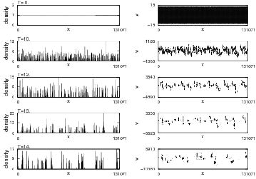
Figure 1: Evolution in configuration and $\mu$ space for the quintic model with $2^{17}$ particles from T=0 to T=14. The initial distribution is a waterbag with velocities in the range (-12.5, 12.5) and a size of about 16,000 Jeans’ lengths.

Figure 2: Consecutive expansions (zooms) on successive small squares selected in the $\mu$ space panels at T=14 for the quintic model. They have the appearance of a random fractal which suggests self-similarity.

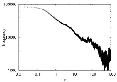
Figure 3: Figure 3. The correlation function at T=14 which shows a scaling region from about 0.3 to about 30, a range of about 2 decades with a scaling exponent $\gamma=.42$.

IV Fractal Measures

It is natural to assume that the apparently self similar structure which develops in the phase plane (see Figs.1,2) as time evolves has fractal geometry, but we will see that things aren’t so simple. In their earlier study of the RF model, Rouet and Feix found a box counting dimension for the particle positions of about 0.6 for an initial waterbag distribution (uniform on a rectangle in the phase plane-see above) and a fractal dimension of about 0.8 in the configuration space (i.e. of the projection of the set of points in $\mu$ space on the position axis). Rouet et al. (1991). As far as we know, Bailin and Shaeffer were the first to suggest that the distribution of galaxy positions are consistent with a bifractal geometry Bialin and Schaeffer (1989) . Their idea was that the geometry of the galaxy distribution was different in the clusters and voids and, as a first approximation, this could be represented as a superposition of two independent fractals. Of course, their analysis was restricted solely to galaxy positions. Since the structures which evolve are strongly inhomogeneous, to gain further insight we have carried out a multi-fractal analysis Halsey et al. (1986) in both the phase plane and the position coordinate.

The multifractal formalism shares a number of features with thermodynamics. To implement it we partitioned each space configuration space and $\mu$ space, into cells of length $l$. At each time of observation in the simulation, a measure $\mu_{i}=N_{i}(t)/N$ was assigned to cell $i$, where $N_{i}(t)$ is the population of cell $i$ at time $t$ and $N$ is the total number of particles in the simulation. The generalized dimension of order $q$ is defined by Halsey et al. (1986)

$$D_{q}=\frac{1}{q-1}\lim_{l\rightarrow 0}\frac{\ln{C_{q}}}{\ln{l}},\quad C_{q}=\Sigma\mu_{i}^{q}.$$ (20)

where $C_{q}(l)$ is the effective partition function Ott (2002), $D_{0}$ is the box counting dimension, $D_{1}$, obtained by taking the limit $q\rightarrow 1$, is the information dimension, and $D_{2}$ is the correlation dimension Halsey et al. (1986)Ott (2002). As $q$ increases above $0$, the $D_{q}$ provide information on the geometry of cells with higher population.

In practice, it is not possible to take the limit $l\rightarrow 0$ with a finite sample. Instead, one looks for a scaling relation over a substantial range of $\ln l$ with the expectation that a linear relation between $\ln{C_{q}}$ and $\ln l$ occurs, suggesting power law dependence of ${C_{q}}$ on $l$. Then, in the most favorable case, the slope of the linear region should provide the correct power and, after dividing by $q-1$, the generalized dimension $D_{q}$. As a rule, or guide, if scaling can be found either from observation or computation over three decades of $l$, then we typically infer that there is good evidence of fractal structure.McCauley (2002) Also of interest is the global scaling index $\tau_{q}$, where ${C_{q}\sim}l^{\tau_{q}}$ for small $l$ . It can be shown that $\tau_{q}$ and $D_{q}$ are related to each other through a Legendre transformation by $D_{q}(1-q)=\tau_{q}$ for $q\neq 1$ Ott (2002). Here we present the results of our fractal analysis of the particle positions on the line (position only) and the plane (position, velocity or $\mu$ space).

If it exists, a scaling range of $l$ is defined as the interval on which plots of $\ln C_{q}$ versus $\ln l$ are linear. Of course, for the special case of $q=1$ we plot $-\Sigma\mu_{i}ln(\mu_{i})$ vs. $ln(l)$ to obtain the information dimension. Ott (2002) If a scaling range can be found, $D_{q}$ is obtained by taking the appropriate derivative. It is well established by proof and example that, for a normal, homogeneous, fractal, all of the generalized dimensions are equal, while for an inhomogeneous fractal, e.g. the Henon attractor, $D_{q+1}\leq{D_{q}}$ Halsey et al. (1986). In the limit of small $l$, the partition function, $C_{q}(l)$, can also be decomposed into a sum of contributions from regions of the inhomogeneous fractal sharing the same point-wise dimension, $\alpha$,

$$C_{q}(l)=\int d\alpha l^{\alpha q}\rho(\alpha)\exp\left[-f\left(\alpha\right)\right]$$ (21)

where $f\left(\alpha\right)$ is the fractal dimension of its support Halsey et al. (1986)Feder (1988)Ott (2002). Then if, for a range of $q$, a single region is dominant, we find a simple relation between the global index, $\tau_{q}$, and $\alpha$,

$$\tau_{q}=\alpha q-f(\alpha).$$ (22)

Recall that a Euclidean metric is imposed on the $\mu$-space. Because, in our units, $\omega_{j}=1,$ we divide it into cells such that $\Delta x=\Delta v$. Then, as $L$ is large ($L\approx 10,000$), so is the extent of the partition in the velocity space. On this scale the initial distribution of particules appears as a line so that the initial dimension is also about unity. In fact, initially the velocity of the particles is a perturbation. It is not large enough to allow particles to cross the entire system in a unit of time. During the initial period the virial ratio rapidly oscillates. After a while the granularity of the system destroys the approximate symmetry of the initial $\mu$-space distribution. Breaking the symmetry leads to the short time dissipative mixing that results in the separation of the system into clusters. Although the embedding dimension is different, the behavior of the distribution of points in configuration space is similar. The initial dimension is nearly one until clustering commences. At this time the dimensions in $\mu$-space and configuration space separate.

As time progresses, however, for the initial conditions discussed above, for $q>0$ typically two independent scaling regimes developed. Of course this is in addition to the trivial scaling regions obtained for very small $l$ , corresponding to isolated points, and to large $l$ on the order of the system size, for which the matter distribution looks smooth. The observed size of each scaling range depended on both the elapsed time into the simulation and the value of $q$. While the length of each scaling regime varied with both $q$ and time, in some instances it was possible to find good scaling over up to four decades in $l$!

Figure 4: Scaling behavior in $\mu$-space. Plots of $\frac{1}{q-1}{\ln{C_{q}}}$ versus $\ln{l}$ are provided for four values of q: a) q=-5, b) q=0. c) q=5, d) q= 10.

In Fig. 4 we provide plots of $\frac{1}{q-1}{\ln{C_{q}}}$ versus $\ln{l}$ in $\mu$-space for four different values of $q$ covering most of the range we investigated ($-5<q<10$). To guarantee that the fractal structure was fully developed, we chose $T=14$ for the time of observation and the initial conditions are those given above. For $q=-5$ and $q=0$ we clearly observe a single, large, scaling range where $0.5<\ln{l}<8$ , corresponding to about three decades in $l$. In the remaining panels (c, d), where we increase $q$ to $5$ , and then $10$, we see a dramatic change. The large scaling range has split into two smaller regions separated at about $l=1.5$, and the slope of the region with larger $l$ has decreased compared with the scaling region on its left ($-1.5<\ln{l}<1.5$). The scaling range with larger $l$, $1.5<\ln{l}<8.5,$ corresponds to just over three decades in $l$. Note that in panels c and d of Fig. 4, the scaling range with larger $l$ is more robust.

Figure 5: Generalized dimension $D_{q}$ vs. $q$ (panel a) and global scaling index $\tau_{q}$vs. $q$ (panel b) in $\mu$-space for the quintic model at T=14 with $q>0$.

Figure 6: Plots of $1/(q-1)ln(C_{q})$ vs $ln(l)$ in configuration ($x$ ) space for the quintic model prepared as above at T=14 are provided for four values of $q$: a) $q=-5$, b) $q=0$, c) $q=5$, d) $q=10$.

Figure 7: Generalized dimension $D_{q}$ vs. $q$ (panel a) and global scaling index $\tau_{q}$vs. $q$ (panel b) in configuration ($x)$space for the quintic model at T=14 with $q>0.$.

Figure 8: Generalized dimension $D_{q}$ vs. $q$ (panel a) and global scaling index $\tau_{q}$vs. $q$ (panel b) in configuration ($x)$space for the quintic model at T=14 with $q<0.$.

Now that we have identified the important scales, we are able to compute the generalized dimension, $D_{q}$, and the global index, $\tau_{q}$. In Fig. 5(a) we plot $D_{q}$ vs $q$ calculated in the $\mu$-space for the quintic model at $T=14$ for $q>0$ for the case of the larger scaling range. As expected, it is a decreasing function and clearly demonstrates multifractal behavior. Although $\mu$ space is two dimensional, $D_{0}$ is about 0.9. While $D_{0}>D_{1}$ is typical for multifractals (information dimension covers the important region), the fact that $D_{q}$ is strictly decreasing suggests greater "fractality" from increasingly overdense regions, i.e. the system is strongly inhomogeneous. In Fig. 5b we plot $\tau_{q}$ versus $q$ in mu space. Two linear regions ($0<q<1$ and $1<q<10$) can be distinguished suggesting bifractal geometry, i.e. a superposition of two fractals with unique values of $\alpha$ and $f(\alpha)$.

We have seen that the one dimensional gravitational system reveals fractal geometry in the higher dimensional $\mu$ space (frequently referred to as phase space in the astronomical literature). Historically self similar behavior was first inferred in gravitational systems by studying the distribution of galaxy locations, i.e in the system’s configuration space, and searching for powerlaw behavior in the correlation function (see above).Bialin and Schaeffer (1989) In common with this approach, we project the mu space distribution on the (position) line to study the geometry of the configuration space. In Fig. 6 a,b,c,d, we provide plots of $1/(q-1)ln(I_{q})$ vs $ln(l)$ in $x$ (configuration) space for the quintic model prepared as above at T=14. In common with the $\mu$-space distribution, for $q=-5$ and $q=0$, there is a single, large scaling region ($-3<ln(l)<3$ for $q=-5$ and $-2<ln(l)<6$ for $q=0$). Similarly, at $q=5$ (c) and $q=10$ (d) the existence of two scaling ranges becomes apparent, $-4<ln(l)<0$ and $0<ln(l)<8$ for $q=5$ (about 3.3 decades), $-3<ln(l)<1$ and $1<ln(l)<8$ for $q=10$ (about 3 decades). Note that the scaling ranges are similar for both the $\mu$ and configuration space, but they are not identical.

In Figure 7 we illustrate the behavior of the generalized dimension $D_{q}$and global index $\tau_{q}$ for the configuration space of the quintic model at $T=14$. Although now the embedding dimension is $d=1$, $D_{0}$ is about $0.7$ so the distribution is definitely fractal. As anticipated from the $\mu$-space distribution, $D_{q}$ is a decreasing function of $q$ so it is also inhomogeneous and multifractal. In Fig. 7b we plot $\tau_{q}$ vs $q$ in configuration space, for the same system. In contrast with the $\mu$-space index, here we observe a nearly linear function with slight convexity (decreasing derivative with respect to $q$). Perhaps this results from the superposition of three linear regions with distinct $\alpha$ and $f(\alpha)$, say with $0<q<1.5$; $1.5<q<7$; $7<q<10$, but this cannot be inferred from the plot without further analysis.

For completeness, in Fig. 8 we examine the behavior of $D_{q}$ and $\tau_{q}$ for $q<0$. In general, negative $q$ is important for revealing the geometry of low density regions (voids). We see that $D_{q}$ has a very unphysical appearance - it is increasing. The source of the problem can be determined by examining the behavior of $\tau_{q}$. It is nearly constant over the range $-10<q<0$ with a value of approximately $\tau_{q}\simeq-1$, implying that the underdense regions are dominated by a single local dimension.

Part of our goal is to compare how fractal geometry arises in a family of related models. So far we have presented results for the quintic, or Q, model. However we have also carried out similar studies of the Rouet-Feix (RF) model, the model without friction (which can be obtained from either of the former by nullifying the first derivative contribution in Eq(14), and simply an isolated system without friction or background. The latter is a purely Newtonian model without a cosmological connection. In Table 1 we list the important characteristic dimensions and exponents for the the quintic model and the model without friction for comparison. While there are similarities in the fractal structure of each of these models, they are not the same. For example in the quintic model the generalized fractal dimension, $D_{q}$, is consistently smaller in each manifold than the corresponding dimension in the model without friction. It is noteworth that the box counting dimension in the configurqtion space of the quintic model is 0.69 compared with 0.90 for the model without friction. Moreover $D_{q}$ is decreasing more rapidly in the quintic model demonstrating stronger inhomogeneity.

Table 1: default

		Quintic model			RF model
$q$		x-space	$\mu$-space		x-space	$\mu$-space
0		$0.69\pm 0.11$	$0.89\pm 0.06$		$0.89\pm 0.02$	$1.14\pm 0.04$
1		$0.64\pm 0.06$	$0.84\pm 0.07$		$0.88\pm 0.04$	$1.17\pm 0.04$
2		$0.62\pm 0.04$	$0.81\pm 0.05$		$0.85\pm 0.04$	$1.13\pm 0.05$

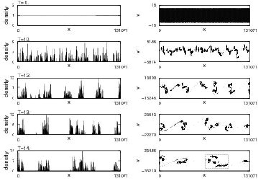
Figure 9: Evolution in configuration and space for the model without friction with $2^{17}$ particles from T=0 to T=14. The initial distribution is a waterbag with velocities in the range (-14, 14) in the dimensionless units employed here and a size of about 10,400 Jeans’ lengths.

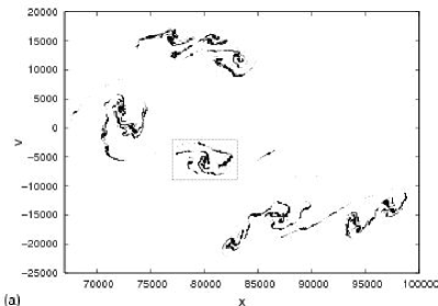
Figure 10: Consecutive expansions (zooms) of successive small squares (square within a square) selected in the $\mu$ space panels at T=14. They also have the appearance of a random fractal which suggests self-similarity.

Figure 11: Generalized dimension $D_{q}$ vs. $q$ (panel a) and global scaling index $\tau_{q}$vs. $q$ (panel b) in configuration ($x)$space for the quintic model at T=14 with $q<0.$

The differences in dynamics between the systems can be seen clearly in Fig. 9 where we show the evolution in configuration and $\mu$-space of the system without friction. In common with the simulations of the quintic model presented above, the initial conditions are a waterbag with velocities sampled independently and confined to ($-12.5,12.5$) in the dimensionless units defined earlier. As before, there are $2^{17}$ particles and the simulation spans $14$ units of the scaled time. The initial size encompasses about 10,400 Jeans lengths. Compared with the quintic model, note that here larger clusters form earlier and have a qualitatively different shape. Due to the absence of “friction” in the dynamics, the velocity spread is larger and there are fewer clusters at each epoch. At T=12 and T=13 the linear structure of the underdense regions (voids) in $\mu$ space connecting the clusters is apparent. Note that they all share a common slope which is due to stretching in the phase plane. However, equation 18 is no longer adequate to provide the line slope. In Fig. 10 we examine the consecutive expansions (zooms) of the large cluster on the right hand side of the $\mu$ space distribution at $T=14$. Once again there is qualitative evidence of stochastic self-similarity Ott (2002) which requires analysis for confirmation. To save space, here we don’t reproduce the plots of $\frac{1}{q-1}{\ln(C_{q})}$ versus $\ln{l}$ in each space. Qualitatively they are similar to the quintic case, but the scaling ranges are less robust.

The behavior of $D_{q}$ and $\tau_{q}$ are similar to that found for the quintic model. However, because the scaling ranges are less robust, there is more noise. For example, in Fig. 11a,b. we plot $D_{q}$ and $\tau_{q}$ versus $q$ in configuration space for the model without friction. Note the similarities with Fig. 6 for the quintic model. The slope of $\tau_{q}$ gradually decreases with increasing $q$. There appears to be three linear segments, from (0, 3), (3, 5), and (5,10) suggesting contributions from three possible fractal scaling regions.

V Discussion of Results

As mentioned earlier, it is well established that, for a regular multifractal, the generalized dimension, $D_{q}$ , is a decreasing function of its argument.Feder (1988)Ott (2002) Therefore, for $q<0$ , it would be incorrect to interpret the simulation results as true generalized dimensions. There must be an alternative explanation for the behavior we observe. The picture for positive $q$ is rather different. The two scaling regions give completely different results. Although one would suspect from the definition of the generalized dimension that the scaling region with smaller $l$ would give the correct one, this is hard to accept since typical plots of the function $D_{q}$ are still increasing until about $q=2$ (not shown) for this range. On the other hand, the second, larger, scaling region manifests a well behaved decreasing function which appears to approach a constant value of $D_{q}\cong 0.63$ for $q\lesssim 10$.

It is interesting that we have observed similar behavior with a well characterized, textbook, fractal that is discussed in numerous sources.Feder (1988) As a test of our computational approach we simulated the multiplicative binomial process. For this multifractal ${\tau_{q}}$ and $D_{q}$ are known precisely.Feder (1988) When we carried out the fractal analysis using the methods described above, we also found two scaling regions. What is most striking is that the scaling region with larger values of $l$ yielded a ${\tau_{q}}$ (and therefore $D_{q}$) which agreed to within numerical error with the theoretical prediction! This type of behavior has been manifested in other simulations of fractal sets. The formation of the smaller scaling range has been attributed to the presence of noise in the data. The existence of a second scaling range has been rigorously shown to arise when Gaussian noise is added to a standard fractal.Schreiber (1997) In the simulation of the multiplicative binomial process, the source of the noise is the random location of the data points within the smallest bins. At this time the source of the apparent noise in the one dimensional gravitational simulations is not precisely known. While it may arise simply from numerical considerations, there are alternative possible explanations. For example, noise may arise from sub-Jeans length fluctuations in the initial data, or from other small scale features of the initial state. In addition to the box-counting approach, other methods based on the correlation function formalism that employ the point-wise dimension can also be used to investigate the fractal properties of the system. It was also used in our investigation and gives similar results to the box counting method reported here.

For $q>0$ we appear to be seeing a similar phenomena to the mutiplicative binomial process or the systems with injected noise.Schreiber (1997) Then how do we explain the surprising and counterintuitive results for $q<0$? Since for negative $q$ we obtain a nearly constant value for $\ {\tau_{q}}$ from each scaling region, it seems safe to assume that a region of the data characterized by a simple fractal behavior has the dominant influence. Moreover, since it only involves $q<0$, it represents the regions of low density, i.e. the voids. Referring to the multifractal formalism, we pointed out earlier that in a region where a single structure dominates,

$$\tau_{q}=\alpha q-f(\alpha),$$ (23)

where $\alpha$ is the strength of the local singularity, or the local pointwise dimension, and $f(\alpha)$ is the Hausdorf dimension of its support.Feder (1988)Ott (2002) Then the computations show that for $q<0$ we must have $\alpha=0$ and $f\cong 0.9$. This suggests that the results for negative $q$ are dominated by regions of such low density that widely separated, ”isolated”, particles are responsible for the spurious behavior of $D_{q}$. At this time this is simply a conjecture which needs to be investigated with further computation.

Finally let’s reconsider the plot of ${\tau_{q}}$ versus $q$ (Fig. 5b) for the larger scaling region with $q>0$. As we mentioned earlier, for $0<q<1.5$ and for $2<q<10$ the curve appears linear with different slopes in each region. This may be the manifestation of bifractality first discussed by Bailin and Shaffer for galaxy positions. The first interval may represent the true fractal structure of the under-dense regions, while the dense clusters are dominant for the larger $q$ values. Bifractal behavior is not unique to gravitational systems. It occurs in a number of well studied model systems, for example as a superposition of two Cantor sets,Shi and Gong (1992) or from the truncation of Levy flights Levy (1954)Nakao (2000) .

VI Conclusions

We have seen that one dimensional models develop hierarchical structure and manifest robust scaling behavior over particular length and time scales. In addition, for a number of reasons, they have an enormous computational advantage over higher dimensional models. First, it is possible to study the evolution of large systems with on the order of $2^{17}$particles per dimension. Second, in contrast with three dimensional N-body simulations, the evolution can be followed for long times without compromising the dynamics. In particular, the force is always represented with the accuracy of the computer - there is no softening. As a consequence it is possible to investigate the prospect for fractal geometry with some confidence.

In common with 3+1 dimensional cosmologies, with the inclusion of the Hubble expansion and the transformation to the comoving frame, both the 1+1 dimensional Quintic and RF Miller and Rouet (2002) models reveal the formation of dense clusters and voids. They also show evidence for bifractal geometry. This may be a consequence of dynamical instability that results in the separation of the system into regions of high and low density. An interesting observation is that the lower bound of the length scale that supports the trivial space dimension of unity in the configuration space grows with time. To the extent that similar behavior occurs in the 3+1 dimensional universe, this lends support for the standard cosmological model on sufficiently large scales. It also suggests that the scale size for homogeneity will grow with time. Eventually this may be testable with observation.

We have seen that the system shows evidence of two nontrivial scaling regions. The type of anomalous behavior of $D_{q}$ and $\tau_{q}$ in the scaling region with a finer partition was also found in the standard multiplicative binomial process with a similar sample size. Even with the large sample size employed here, this would suggest that it is a finite size effect. In that respect it will be interesting to perform simulations dealing directly with the distribution function given by the Vlasov equation. Then the low density region will be well described. This may also be true for the region of negative $q$ where a fractal analysis forces us to conclude that the point-wise dimension vanishes. Computations with different boundary conditions reveal similar behavior, but this work is only in the preliminary stages. Future work will include the investigation of the influence of correlation in the initial conditions, the consideration of initial conditions of the type employed in current cosmological N-body simulations Springiel et al. (2006), and the study of the fractal geometry of the under and over dense regions. We plan to compare out findings with three dimensional studies of the distribution of voids and halos Gaite (2007).

In addition to these important features, the one dimensional simulations unequivocally demonstrate that the essential structure formation is taking place in the $\mu$ space (phase space for astronomers). Thus the apparent fractal geometry that we observe in configuration space is simply a shadow (projection) of the higher dimensional structure. The development of structure in $\mu$ space and its apparent fractal geometry may be the most significant result of these studies. Since evolution in the six dimensional $\mu$ space of the observable universe is beyond our current capability, the study of lower dimensional models is an important guide for understanding the important features of the higher dimensional evolution. For example, we have shown analytically that dynamical “stretching” of the $\mu$ space geometry is responsible for the formation of underdense regions (voids) and, consequently, the concentration of mass in regions of decreasing area. We are currently extending this analysis to the study of structure formation in the more realistic 3+1 dimensional manifold.

References

- de Vaucouleurs (1970) G. de Vaucouleurs, Science 167, 1203 (1970).
- Peebles (1993) P. J. E. Peebles, Principles of Physical Cosmology (Princeton University Press, Princeton, NJ, 1993).
- Pecker and Narlikar (2006) J.-C. Pecker and J. Narlikar, Current Issues in Cosmology, volume 167 (Cambridge University Press, Cambridge, UK, 2006).
- Jones et al. (2004) B. Jones, V. Martinez, E. Saar, and V. Trimble, Reviews of Modern Physics 76, 1211 (2004).
- Mandelbrot (1982) B. Mandelbrot, The Fractal Geometry of Nature (Freeman, San Francisco, 1982).
- Labini et al. (1998) F. S. Labini, M. Montuori, and L. Pietronero, Physics Reports 293, 61 (1998).
- McCauley (2002) J. L. McCauley, Physica A 309, 183 (2002).
- Balian and Schaeffer (1989) R. Balian and R. Schaeffer, Astronomy and Astrophysics 226, 373 (1989).
- Ott (2002) E. Ott, Chaos in Dynamical Systems (Cambridge, Cambridge, UK, 2002).
- chan Hwang and Noh (2006) J. chan Hwang and H. Noh, MNRAS p. in press (2006).
- de Vega and Sanchez (2000) H. de Vega and N. Sanchez, Phys. Lett. B 490, 180 (2000).
- Grujic (2005) P. V. Grujic, Astrophysics and Space Science 295, 363 (2005).
- Bagla (2005) J. Bagla, Current Science 88, 1088 (2005).
- Bertschinger (1998) E. Bertschinger, Annual Review of Astronomy and Astrophysics 36, 599 (1998).
- Mann and Chak (2002) R. B. Mann and P. Chak, Physical Review E 65, 026128 (2002).
- Rouet et al. (1990) J.-L. Rouet, M. R. Feix, and M. Navet, in Vistas in Astronomy 33, edited by A. Heck (Pergamon, 1990), pp. 357–370.
- Rouet et al. (1991) J.-L. Rouet, E. Jamin, and M. R. Feix, in Applying Fractals in Astronomy, edited by A. Heck and J. M. Perdang (Springer-Verlag, Berlin, 1991), pp. 161–179.
- Fanelli and Aurell (2002) D. Fanelli and E. Aurell, Astronomy and Astrophysics 395, 399 (2002).
- Kofman et al. (1992) L. A. Kofman, D. Pogosyan, S. F. Shandarin, and A. L. Melott, 393, 437 (1992).
- Shandarin and Zeldovich (1989) S. F. Shandarin and Y. B. Zeldovich, Reviews of Modern Physics 61, 185 (1989).
- Tatekawa and Maeda (2001) T. Tatekawa and K. Maeda, Astrophysical Journal 547, 531 (2001).
- Gurbatov et al. (1997) S. N. Gurbatov, S. I. Simdyankin, U. F. E. Aurell, and G. Toth, 344, 339 (1997).
- Koyama and Konishi (2001) H. Koyama and T. Konishi, Physics Letters A 279, 226 (2001).
- Koyama and Konishi (2002) H. Koyama and T. Konishi, Euro Physics Letters 58, 356 (2002).
- B.N.Miller and Rouet (2002) B.N.Miller and J.-L. Rouet, Physical Review E 65, 056121 (2002).
- Aurell et al. (2003) E. Aurell, D. Fanelli, S. N. Gurbatov, and A. Y. Moshkov, Physica D 186, 171 (2003).
- Weissert (1997) T. P. Weissert, The Genesis of Simulation in Dynamics (Springer-Verlag, New York, 1997).
- Cohen and Lecar (1968) L. Cohen and M. Lecar, Bull. Astr. 3, 213 (1968).
- Hohl (1967) F. Hohl, Ph.D. thesis, College of William and Mary (1967).
- Wright et al. (1982) H. Wright, B. Miller, and W. Stein, Ap. Space Sci. 84, 421 (1982).
- Yawn and Miller (1997a) K. Yawn and B. Miller, Phys. Rev. E 56, 2429 (1997a).
- Yawn and Miller (1997b) K. Yawn and B. Miller, Phys. Rev. Letters 79, 3561 (1997b).
- Posh et al. (1993) H. A. Posh, H. Narnhofer, and W. Thirring, Physica A 194, 482 (1993).
- Milanovic et al. (1998) L. Milanovic, H. Posch, and W. Thirring, Phys. Rev. E 57, 2763 (1998).
- Milanovic et al. (2006) L. Milanovic, H. A. Posch, and W. Thirring, Journal of Statistical Physics 124, 843 (2006).
- Rouet and Feix (1999) J.-L. Rouet and M. R. Feix, Physical Review E 59, 73 (1999).
- B.Miller et al. (2005) B.Miller, K.Yawn, and B.Maier, Physics Letters A 346, 92 (2005).
- Binney and Tremaine (1987) J. Binney and S. Tremaine, Galactic Dynamics (Princeton University Press, Princeton, NJ, 1987).
- Press et al. (1992) W. Press, B. Flannery, S. Teukolsky, and W. Vetterling, Numerical Recipes in C: The Art of Scientific Computing (Cambridge University Press, Cambridge, 1992).
- Bialin and Schaeffer (1989) R. Bialin and R. Schaeffer, Astronomy and Astrophysics 226, 373 (1989).
- Halsey et al. (1986) T. C. Halsey, M. H. Jensen, L. P. Kadanoff, I. Procaccia, and B. Shraiman, Physical Review A 33, 1141 (1986).
- Feder (1988) J. Feder, Fractals (Plenum, New York, 1988).
- Schreiber (1997) T. Schreiber, Physical Review E 56, 274 (1997).
- Shi and Gong (1992) Y. Shi and C. Gong, Physical Review A 46, 8009 (1992).
- Levy (1954) P. Levy, Memoir. Sci. Math. Fasc. (Gauthier-Villas, Paris, 1954).
- Nakao (2000) H. Nakao, Physics Letters A 266, 282 (2000).
- Miller and Rouet (2002) B. N. Miller and J. L. Rouet, Physical Review E 65, 056121 (2002).
- Springiel et al. (2006) V. Springiel, C. S. Frenk, and S. D. M. White, Nature 440, 1137 (2006).
- Gaite (2007) J. Gaite, Astrophysical Journal p. in press (2007).