LAMINATED WAVE TURBULENCE: GENERIC ALGORITHMS II

Abstract

The model of laminated wave turbulence puts forth a novel computational problem - construction of fast algorithms for finding exact solutions of Diophantine equations in integers of order $10^{12}$ and more. The equations to be solved in integers are resonant conditions for nonlinearly interacting waves and their form is defined by the wave dispersion. It is established that for the most common dispersion as an arbitrary function of a wave-vector length two different generic algorithms are necessary: (1) one-class-case algorithm for waves interacting through scales, and (2) two-class-case algorithm for waves interacting through phases. In our previous paper we described the one-class-case generic algorithm and in our present paper we present the two-class-case generic algorithm.

PACS numbers: 47.10.-g, 47.27.De, 47.27.T, 02.60.Pn

1 INTRODUCTION

The most general problem setting of the wave turbulence theory can be regarded in the form of a nonlinear partial differential equation

$$\mathcal{L}(\psi)=\varepsilon\mathcal{N}(\psi)$$

where $\mathcal{L}$ and $\mathcal{N}$ denote linear and nonlinear part of the equation correspondingly, the linear part has the standard wave solutions of the form

$$\varphi=A\exp{i[\vec{k}\vec{x}-\omega t]},$$

where the amplitude $A$ may depend on space variables but not on time, and a small parameter $\varepsilon$ shows that only resonant wave interactions are taken into account. The dispersion function $\omega=\omega(\vec{k})$ can be easily found by substitution of $\varphi$ into the linear part of the initial PDE, $\mathcal{L}(\varphi)=0,$ while $\partial_{t}\leftrightarrow i\omega\quad\mbox{and}\quad\partial_{x_{s}}\leftrightarrow ik_{s},$ and resonance conditions have the form

$$\begin{cases}\omega(\vec{k}_{1})\pm\omega(\vec{k}_{2})\pm...\pm\omega(\vec{k}_{n})=0,\\ \vec{k}_{1}\pm\vec{k}_{2}\pm...\pm\vec{k}_{n}=0.\end{cases}$$ (1)

for $n$ interacting waves with wave-vectors $\vec{k}_{i},\ \ i=1,2,...,n$. For most physical applications it is enough to regard $n=3$ or $n=4$, and the most common form of dispersion function is

$$\omega=\omega(|\vec{k}|),\ \ \ \ |\vec{k}|=\sqrt{m^{2}+n^{2}}\quad\mbox{for}\quad\vec{k}=(m,n)$$

(for instance, capillary, gravitational and surface water waves, planetary waves in the ocean, drift waves in tokamak plasma, etc.)

The model of laminated wave turbulence[1] describes two co-existing layers of turbulence - continuous and discrete - which are presented by real and integer solutions of Sys.(1) correspondingly. The continuous layer is described by classical statistical methods[2] while for the discrete layer new algorithms have to be developed. It was shown in[3] that an arbitrary integer lattice $(m,n)$, each node of the lattice denoting a wave-vector $\vec{k}=(m,n)$, can be divided into some clusters (classes) and there are two types of solutions of Sys.(1): those belonging to the same class and those belonging to different classes. Mathematically, a class is described as a set of wave-vectors for which the values of the dispersion function have the same irrationality. For instance, if the dispersion function has the form $\omega=\sqrt{m^{2}+n^{2}}$, then a class is described as follows:

$$\{m_{i},n_{i}\}:\ \sqrt{m_{i}^{2}+n_{i}^{2}}=\gamma_{i}\sqrt{q}$$

where $\gamma$ is a natural number and $q$ is a square-free integer. Physically, it means that waves are interacting over the scales, that is, each two interacting waves generate a wave with a wavelength different from the wave lengths of the two initial waves. Interactions between the waves of different classes do not generate new wavelengths but new phases.

In our preceding paper[4] we presented a generic algorithm for computing all integer solutions of Sys.(1) within one class. Four-wave interactions among 2-dimensional gravitational water waves were taken as the main example, in this case Sys.(1) takes form:

$$\begin{cases}{(m_{1}^{2}+n_{1}^{2})}^{1/4}+{(m_{2}^{2}+n_{2}^{2})}^{1/4}={(m_{3}^{2}+n_{3}^{2})}^{1/4}+{(m_{4}^{2}+n_{4}^{2})}^{1/4}\\ m_{1}+m_{2}=m_{3}+m_{4}\\ n_{1}+n_{2}=n_{3}+n_{4}\\ \end{cases}$$ (2)

and classes are defined as $Cl_{q}=\{\gamma^{4}q\}$, where $q$, called class index, are all natural numbers containing every prime factor in degree smaller $4$ and $\gamma$, called weight, all natural numbers. It can be proven that if all 4 wave-vectors constructing a solution of Sys.(2) do not belong to the same class, then the only possible situation is following: all the vectors belong to two different classes $Cl_{q_{1}},Cl_{q_{2}}$ and the first equation of Sys.(2) can be rewritten then as

$$\gamma_{1}\sqrt[4]{q_{1}}+\gamma_{2}\sqrt[4]{q_{2}}=\gamma_{1}\sqrt[4]{q_{1}}+\gamma_{2}\sqrt[4]{q_{2}}$$ (3)

with some $\gamma_{1},\gamma_{2}\in\hbox{\Sets N}$ and $q_{1},q_{2}$ being class indexes. In the present paper we deal with this two-class case.

2 COMPUTATIONAL PRELIMINARIES

As in the previous paper [4], we are going to find all solutions of Eq.(2) in some finite domain $D$, i.e. $|m_{i}|,|n_{i}|\leq D$ for some $D\in\hbox{\Sets N}$. The first case has been studied for $D=1000$, where $\pi_{cl}(10^{3})=384145$ classes have been encountered. The straightforward approach, not making use of classes, consumes, as for the first case, at least $O(D^{5})$ operations and is out of question (see [4], Sec.3.2.1 for discussion of this point).

Straightforward application of classes also does not bring much. The Eq.(3) is now trivial - but classes are interlocked through linear conditions. Even if for each pair of classes we could detect interlocking and find solutions, if any, in $O(1)$ operations (which is probably the case, though we did not prove it), the overall computational complexity is at least $\pi_{cl}(D)^{2}$ - i.e. not much less than $O(D^{4})$. For $D=1000$ this implies $1.5\cdot 10^{11}$ pairwise class matches which is outside any reasonable computational complexity limits.

The trouble with this approach - as, for that matter, with virtually any algorithm consuming much more computation time than the volume of its input and output data implies - is, that we perform a lot of intermediary calculations, later discarded. We develop an algorithm performing every calculation with a given item of input data just once (or a constant number of times). First of all we notice that Eq.(3) can be rewritten as

$$\begin{cases}{(m_{1L}^{2}+n_{1L}^{2})}^{1/4}={(m_{1R}^{2}+n_{1R}^{2})}^{1/4}=\gamma_{1}\sqrt[4]{q_{1}}\\ {(m_{2L}^{2}+n_{2L}^{2})}^{1/4}={(m_{2R}^{2}+n_{2R}^{2})}^{1/4}=\gamma_{2}\sqrt[4]{q_{2}}\\ m_{1L}-m_{1R}=-m_{2L}+m_{2R}\\ n_{1L}-n_{1R}=-n_{2L}+n_{2R}\\ \end{cases}$$ (4)

where $q_{1},q_{2}$ are two different class indexes and $\gamma_{1},\gamma_{2}$ - the corresponding weights.

Definition.

For any two decompositions of a number $\gamma_{1}^{4}q$ into a sum of two squares (see (4)) the value $\delta_{m}=m_{L}-m_{R}$ is called $m$-deficiency, $\delta_{n}=n_{L}-n_{R}$ is called $n$-deficiency and $\vec{\delta}_{m,n}=(\delta_{m},\delta_{n})$ - deficiency point.

We immediately see that for two interacting waves their deficiencies must be equal: $\delta_{1m}=m_{1L}-m_{1R}=-m_{2L}+m_{2R}=\delta_{2m},\quad\delta_{1n}=n_{1L}-n_{1R}=-n_{2L}+n_{2R}=\delta_{2n}$. For a given weight $\gamma$, every two decompositions of $\gamma^{4}q$ into a sum of two squares yield, in general, four deficiency points with $\delta_{m},\delta_{n}\geq 0$. Consider unsigned decompositions $m_{L},m_{R},n_{L},n_{R}\geq>0$. Assuming $m_{L}\geq m_{R},n_{L}\leq n_{R}$ the four points are $(m_{L}+m_{R},n_{L}+n_{R}),\quad(m_{L}+m_{R},-n_{L}+n_{R}),\quad(m_{L}-m_{R},n_{L}-n_{R}),\quad(m_{L}-m_{R},-n_{L}+n_{R})$ and four (symmetrical) points in each of the other three quadrants of the $(m,n)$ plane.

Definition.

The set of all deficiency points of a class for a given weight, $\Delta^{\gamma}_{q}$, is called its $\gamma$-deficiency set. The set of all deficiency points of a class, $\Delta_{q}$, is called its deficiency set.

The objects defined above play the main role in our algorithm, so we compute as an illustrative example the for the number 50. The number $50$ has three decompositions into sum of two squares, namely, $50=1^{2}+7^{2}=5^{2}+5^{2}=7^{2}+1^{2}$, and nonnegative deficiency points of decomposition pairs are $(5,5;7,1),\quad(5,5;1,7),\quad(1,7;7,1).\quad$ They constitute a subset of the deficiency set $\Delta^{1}_{50}$, namely, the 12 points with $m\geq 0,n\geq 0$. In each of three other quadrants of the $(m,n,)$ plane there lie 36 more points of this set, symmetrical to the ones shown with respect to the coordinate axes.

The crucial idea behind the algorithm of this paper is very simple and follows immediately from the exposition above:

Sys.(4) has a solution with vectors belonging to the two different classes $Cl_{q_{1}},Cl_{q_{2}}$ if and only if their deficiency sets have a non-void intersection, $\Delta_{q_{1}}\cap\Delta_{q_{2}}\neq\emptyset$, i.e. some elements belong to both classes.
.

3 ALGORITHM DESCRIPTION

Calculation of relevant class indexes $q$ by a sieve-like procedure, admissible weights $\gamma$ and decomposition of $\gamma^{4}q$ into sum of two squares have all been treated in full detail in [4]. One new feature we introduced here is, that immediately after generating the array of class bases $q$ we purge away those which, whatever the admissible weight $\gamma$, do not have a decomposition into a a sum of two squares $\gamma^{4}q=m^{2}+n^{2}$ with both $m\leq D,\quad n\leq D$. For the problem considered in [4] this would be superfluous because virtually all these classes have been anyhow filtered away according to another criterium ($\mathcal{M}(q)=1,\quad Dec(q)\leq 4$) which does not apply here. In this way we exclude 100562 classes from the 384145 which the sieving procedure returns.

Evidently for any deficiency point $\vec{\delta}_{m,n}$ inequalities $|\delta_{m}|\leq 2D,\quad|\delta_{n}|\leq 2D$ hold. And if deficiency sets of two classes have a non-void intersection, they also have an intersection over points with non-negative $|\delta_{m}|,|\delta_{n}|$. So we start with declaring a two-dimensional array $arDeficiency(0..2D,0..2D)$ of type byte which serves storing and processing deficiency sets of the classes. The array is initialized with all zeroes.

3.1 The Five-Pass Procedure

3.1.1 Pass 1: Marking deficiency points

In the first pass for every class $q$ in the main domain $D$ we generate its deficiency set $D_{q}$. Notice that after generating deficiency set of the class for each weight $\gamma$ and uniting them we must check for doubles and eventually get rid of them. Next, for every deficiency point $(\delta_{m},\delta_{n})$ of the class we increment the value of the corresponding element of the array by 1, except elements with value 255 whose values are not changed.

3.1.2 Pass 2: Discarding non-interacting classes

In the second pass we generate deficiency sets once more and for every point of the deficiency set of a class check the values of the corresponding point of $arDeficiency$. If all these values are equal to $1$, no waves of the class participate in resonant interactions and the class is discarded from further considerations.

For the problem considered this pass excludes just a few ($313$) classes, so the time gain is very modest. However, we include this step into the presentation for two reasons. First of all, it had to be done as no possibility of reducing the number of classes considered as much as possible and as soon as possible (before the most time-consuming steps) may be neglected. Second, though giving not much gain for solution of the problem at hand, this elimination techniques may play a major role in further applications of our algorithm.

3.1.3 Pass 3: Linking interaction points to interacting vectors

In the third pass we generate a more detailed deficiency set for each class, i.e. for all classes not discarded in the previous pass: for every deficiency point $\vec{\delta}_{m,n}$ we store $q,\gamma,m_{L},n_{L},m_{R},n_{R}$. We do not discard duplicates as we did in the previous two passes. Then we revisit the corresponding points of $arDeficiency$ and to each point whose value is larger than $1$ link the structure $(q,\gamma,m_{L},n_{L},m_{R},n_{R})$ described above.

3.1.4 Pass 4: Gathering interaction points

In the fourth pass we go through the array $arDeficiency$ once more and store every point with value greater than one in an array $arDeficiencySol(1..2D,0..1)$. We also relink structures linked to deficiency points to corresponding points of the new array.

3.1.5 Pass 5: Extracting solutions

The four passes above leave us with an array of points $\vec{\delta}_{m,n}$ and to each of these points a list of structures $(q^{i},\gamma^{i},m^{i}_{L},n^{i}_{L},m^{i}_{R},n^{i}_{R})$ is linked (no less than two different $q^{i}$). In general, a linked list is here most appropriate. Every combination of two structures linked to the same point and having different $q^{i}$ yields a solution of Sys.(2). From every solution found, we obtain four solutions changing signs of $m^{i},n^{i}$ in the general case, i.e. for $m^{i},n^{i}$ nonzero.

Notice that theoretically we could skip Pass 4 and extract solutions directly from the array $arDeficiency$. However, this is not reasonable for implementation reasons, and Pass 4 is not very time-consuming.

3.1.6 Implementation remarks.

Implementing the algorithm described above, we took a few language-specific shortcuts that will be briefly described here.

Passes 1 and 2 have been implemented one-to-one as described above. However, manipulating linked lists in VBA involves considerable overhead and for the problem considered in this paper we do not need the complete functionality of linked lists, i.e. inserting into/deleting from intermediate positions of the list. Our main data structure for Pass 3-5 is a simple two-dimensional array arSolHalves($1..N_{MNdef},0..7$) and in a single line of this array we store:

• the class base $q$;

• the coordinates of deficiency point $d_{m},d_{n}$;

• the coordinates of two wave vectors belonging to this deficiency point;

• the index in the array arSolHalves of the next line belonging to the same deficiency point.

which is demonstrated in Fig.1 below.

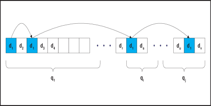
Figure 1: Array simulation of deficiency point lists: the overall array/list structure

Here, $N_{MNdef}$ is the number of $m,n$-vectors linked to all deficiency points to which vectors belonging to two or more classes belong ($6692832$ for $D=1000$). We generate the deficiency set of each class and fill all members of this line of the array except the last one in the process, deficiency point by deficiency point. The last member is filled later and in the following way.

For this pass we also declare an auxiliary array arDeficiencesPrev(1..$2D$, 1..$2D$) initialized with zeroes. Having added a new line $\{q,d_{m},d_{n},m_{1L},n_{1L},m_{1R},n_{1R},0\}$ to arSolHalves, we look up the value $ind_{d_{m},d_{n}}$of arDeficiencesPrev($d_{m},d_{n}$). If it is zero (this deficiency point being visited the first time) we just assign this point the value of the index of the new line in the array arSolHalves. Otherwise we first assign arSolHalves($ind_{d_{m},d_{n}}$, 7) the value of the current line’s index in arSolHalves, then write this number to arDeficiencesPrev($d_{m},d_{n}$) (see Fig.2).

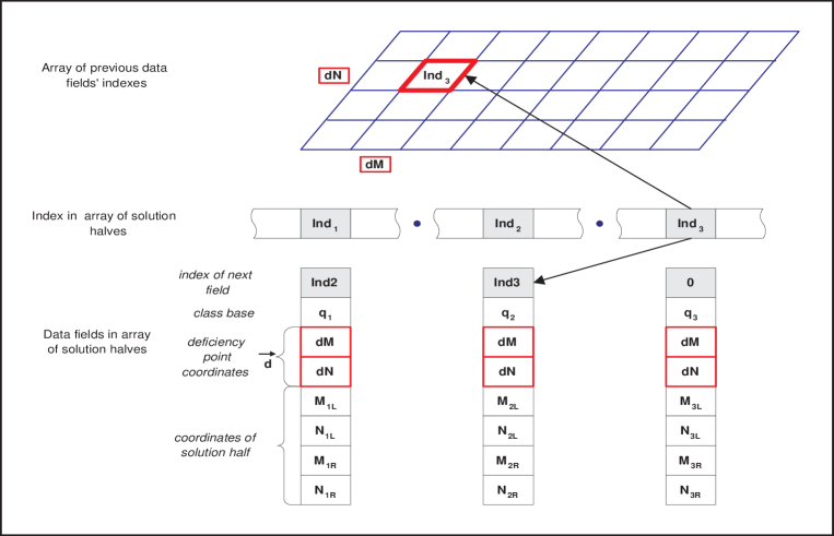
Figure 2: Array simulation of deficiency point lists: data fields in detail.

A numerical example for this procedure is given in Table 1. In this way, the array index of the next ”list” member is stored with the previous one, except evidently the last one, where the corresponding field stays zero.

$Index$	$q$	$d_{m}$	$d_{n}$	$m_{L}$	$n_{L}$	$m_{R}$	$n_{R}$	$NextIndex$
1	1	1	1	0	1	1	0	117
117	1	1	1	-119	120	120	-119	1241
1241	4	1	1	-1	2	2	-1	2921
2921	8	1	1	-2	3	3	-2	4958
4958	12	1	1	-3	4	4	-3	8107
8107	19	1	1	-4	5	5	-4	10304
…	…	…	…	…	…	…	…	…
6692782	273559	1	1	-995	996	996	-995	6692802
6692802	273567	1	1	-996	997	997	-996	6692816
6692816	273575	1	1	-997	998	998	-997	6692828
6692828	273580	1	1	-998	999	999	-998	6692832
6692832	273583	1	1	-999	1000	1000	-999	0

Table 1. A few lines of the table containing solution halves for the deficiency point $\vec{d}=(1,1)$ (beginning and end of the sequence).

3.2 Computational Complexity

Consider computational complexity of these steps.

3.2.1 Pass 1

For a single class index $q$ and weight $\gamma$, generating deficiency points in the first step consumes $\leq O(\log^{2}(\gamma^{4}q))$ operations because every number $X$ has no more than $O(\log X)$ decompositions into two squares which we combine pairwise to find deficiency points. Decompositions themselves can be found in $O(\log(\gamma^{4}q))$ time[5]. There are $(D/q)^{1/4}$ admissible weights to class index $q$, so the overall complexity for a class can be estimated from above as $\log^{2}DD^{1/4}$. Merging deficiency points into $\Delta_{q}$ can be done in $O(X\log X)$ time for number of points X, i.e. no more than $O(\log^{2}DD^{1/4}\log(\log^{2}DD^{1/4}))=O(\log^{3}DD^{1/4})$

Taking a rough upper estimate for the number of classes $O(D^{2})$, we obtain an estimate $O(\log^{3}DD^{2.25})$. Incrementing the points of $arDeficiency$ is linear on the point number of the set $\Delta_{q}$ and need not be considered for computational complexity separately.

3.2.2 Pass 2

The same complexity estimate holds for the second pass. Notice that, having enough memory, or using partial data loading/unloading similar to that used in [6], we could preserve deficiency sets calculated on the first pass and not recalculate them here. However, this would not significally improve the overall computational complexity of the algorithm.

We can not give an a priori estimate for the number of classes discarded at the second pass, so we ignore it and hold the initial rough upper estimate $O(D^{2})$ for the number of classes in our further considerations.

3.2.3 Pass 3

In the third pass, to every point $\delta_{m,n}$ (no more than $O(\log^{2}DD^{1/4})$ of them) we link the values $(q^{i},\gamma^{i},m^{i}_{L},n^{i}_{L},m^{i}_{R},n^{i}_{R})$ for which this point has been struck. This, as well as linking to the points of $arDeficiency$ is, clearly, linear on the number of points and does not raise the computational complexity.

3.2.4 Pass 4

Complexity of the fourth pass can be estimated as follows. Suppose the worst case, i.e. no classes are discarded at step 2 and every deficiency point is a solution point, i.e. for every $\vec{\delta}_{m,n}=(\delta_{m},\delta_{n})$ no less than two classes have deficiency points with the same $d_{m},d_{n}$. Then we must make no more than $O(\log^{2}DD^{2.25})$ entries into the new array $arDeficiencySol$. We must relink no more than the mean of $O(\log^{2}D)$ structures per point, which gives an upper estimate of $O(\log^{4}DD^{2.25})$ time for the pass. However, remember that the estimate for the deficiency point number has been made on the assumption that all $(m^{i}_{L},n^{i}_{L},m^{i}_{R},n^{i}_{R})$ generate distinct deficiency points. In simple words, for every point linked to $X>1$ structures we obtain $X-1$ less solution points. Now elementary consideration allow us to improve the estimate to $O(\log^{2}DD^{2.25})$ time.

3.2.5 Pass 5

We did not manage to obtain a reasonable estimate for the computational complexity of the fifth step. For the worst case of all structures grouped at a single point, the estimate is $O(\log^{4}DD^{4.5})$ - but this is not realistic. If the number of solution points is $O(\log^{2}DD^{2.25})$ and the number of linked deficiencies is bounded by some number $c$, then we can make an estimate $O(c^{2}\log^{2}DD^{2.25})$. This, however, is also not quite the case as our numerical simulations show). However, this last step deals with solution extraction and extracts them in linear time per solution. Any algorithm solving the problem has to extract solutions, so we can be sure that our step 5 is optimal - even without any estimate of its computational complexity. Summing up, we obtain the overall upper estimate of computational complexity $O(\log^{3}DD^{2.25})$ reached at steps $1$ and $2$ plus the time needed for solution extraction.

4 DISCUSSION

Our algorithm has been implemented in the VBA programming language; computation time (without disk output of solutions found) on a low-end PC (800 MHz Pentium III, 512 MB RAM) is about 10 minutes. Some overall numerical data is given in the two Figures below. The number of solutions for the 2-class-case depending on the partial domain is shown in the Fig.3. Both curves are almost ideal cubic lines. Very probably they are cubic lines asymptotically - the question is presently under study.

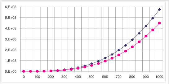
Figure 3: Number of solutions in partial domains $m_{i},n_{i}\leq D$ (curve marked diamonds) and $m_{i}^{2}+n_{i}^{2}\leq D^{2}$ (curve marked circles), $D=50,100,...1000$.

Partial domains chosen in Fig.3 are of two types: squares $m_{i},n_{i}\leq D$, just for simplicity of computations, and circles $m_{i}^{2}+n_{i}^{2}\leq D^{2}$, more reasonable choice from physical point of view (in each circle all the wave lengths are $\leq D$). The curves in the Fig.3 are very close to each other in the domain $D\leq 500$ though number of integer nodes in a corresponding square is $D^{2}$ and in a circle with radius $D$ there are only $\pi D^{2}/4$ integer nodes. This indicates a very interesting physical phenomenon: most part of the solutions is constructed with the wave vectors parallel and close to either axe $X$ or axe $Y$.

On the other hand, the number of solutions in rings $(D-50)^{2}<m_{i}^{2}+n_{i}^{2}\leq D^{2}$ (corresponds to the wavelengths between $D-50$ and $D$) grows nearly perfectly linearly. Of course the number of solutions in a circle is not equal to the sum of solutions in its rings: a solution lies in some ring if and only if all its four vectors lie in that same ring. That is, studying solutions in the rings only, one excludes automatically a lot of solutions containing vectors with substantially different wave lengths simultaneously, for example, with wave vectors from the rings $D-50$ and $D+100$. This ”cut” sets of solutions can be of use for interpreting of the results of laboratory experiments performed for investigation of waves with some given wave lengths (or frequencies) only.

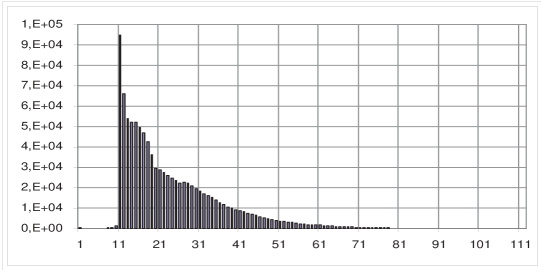
Figure 4: The multiplicities histogram.

Another important characteristic of the structure of the solution set is multiplicity of a vector which describes how many times a given vector is a part of some solution. The multiplicity histogram is shown in Fig.4. On the axis $X$ the multiplicity of a vector is shown and on the axis $Y$ the number of vectors with a given multiplicity. The histogram of multiplicities is presented in Fig. 4, it has been cut off - multiplicities go very high, indeed the vector (1000,1000) takes part in 11075 solutions.

Similar histograms computed for different 1-class-cases show that most part of the vectors, $70-90\%\%$ for different types of waves, take part in one solution, e.g. they have multiplicity 1. This means that triads or quartets are, so to say, the ”primary elements” of a wave system and we can explain its most important energetic characteristics in terms of these primary elements. The number of vectors with larger multiplicities decreases exponentially when multiplicity is growing. The very interesting fact in the 2-class-case is the existence of some initial interval of small multiplicities, from 1 to 10, with very small number of corresponding vectors. For instance, there exist only 7 vectors with multiplicity 2. Beginning with multiplicity 11, the histogram is similar to that in the 1-class-case.

This form of the histogram is quite unexpected and demonstrates once more the specifics of the 2-class-case compared to the 1-class-case. As one can see from the multiplicity diagram in Fig. 4, the major part in 2-class-case is played by much larger groups of waves with the number of elements being of order 40: each solution consists of 4 vectors, groups contain at least one vector with multiplicity 11 though some of them can take part in the same solution. This sort of primary elements can be a manifestation of a very interesting physical phenomenon which should be investigated later: triads and quartets as primary elements demonstrate periodic behavior and therefore the whole wave system can be regarded as a quasi-periodic one. On the other hand, larger groups of waves may have chaotic behavior and, being primary elements, define quite different way of energy transfer through the whole wave spectrum.

References

- [1] E.A. Kartashova. JETP Letters (83) 7, 341 (2006)
- [2] V.E. Zakharov, V.S. L’vov, G. Falkovich. Kolmogorov Spectra of Turbulence (Series in Nonlinear Dynamics, Springer, 1992)
- [3] E.A. Kartashova. AMS Transl. (182), 2, 95 (1998)
- [4] E.A. Kartashova, A.P. Kartashov. Int. J. of Modern Physics C, to appear (2006)
- [5] J.M. Basilla. Proc. Japan. Acad. 80, Ser. A, 40 (2004)
- [6] A.P. Kartashov, R. Folk ”Delaunay triangulations in the plane with storage requirements”, Int. J. of Computational Physics, 6, pp.639-649