A new approach to the absorbing boundary conditions for the Schrödinger type equations

Abstract

By the multiple-scale method some new approximate absorbing boundary conditions for the Schrödinger type equations are obtained.

I Introduction

We will consider the construction of the absorbing boundary conditions for the Schrödinger type equations (subscripts are used for the derivative with respect to the corresponding variable)

$$\mathrm{i}u_{x}+\beta(x)u_{yy}+\nu(x,y)u=0\,,$$ (1)

which arise in numerous quantum-mechanical problems and as approximate models for the wave propagation in the parabolic equation method and its generalizations bab-bul . For calculating solutions of this equation in unbounded domains it is essential to introduce boundary conditions at the boundaries of the computational domain which model the free transmission of the waves through these boundaries. As these boundary conditions must minimize the amplitudes of waves reflected from boundaries, they are called absorbing boundary conditions eng-maj .

There is a significant number of works where the problem of constructing of such boundary conditions was considered. The main approaches in these works consist either in factorization of the differential operator of the equation under consideration into pseudodifferential factors, each of which describes the unidirectional wave propagation eng-maj ; shib ; kus and use the differential approximations of these factors for the formulation of the boundary conditions, or in formulation of the absorbing boundary conditions as the matching condition with the free space solution outside of the computational domain (for the Eq. (1) see the paper bas-pop .

As is known, the approximate description of the unidirectional propagation of the waves can be obtained by the generalized multiple-scale method nay , which in particular cases gives the same results as the WKB or ray method. In this approach the algebraic factorization of the Hamilton-Jacobi equation replaces the factorization of the differential operator. In the simplest case this approach was reported in tr .

II Derivation of the boundary conditions

To apply the multiple-scale method nay to the Eq. (1) we introduce the slow variables $X=\epsilon x$, $Y=\epsilon y$, the fast variable $\eta=(1/\epsilon)\theta(X,Y)$, where $\epsilon$ is a small parameter, change the partial derivatives in Eq. (1) for the prolonged ones by the rules

$$\frac{\partial}{\partial x}\rightarrow\epsilon\frac{\partial}{\partial X}+\theta_{X}\frac{\partial}{\partial\eta}\,,\qquad\frac{\partial}{\partial y}\rightarrow\epsilon\frac{\partial}{\partial Y}+\theta_{Y}\frac{\partial}{\partial\eta}\,,$$

and substitute in the obtained equation the expansion

$$u=u_{0}+\epsilon u_{1}+\ldots\,.$$

Equating coefficients of like powers of $\epsilon$, we obtain at $O(\epsilon^{0})$ the representation

$$u_{0}=A_{0}(X,Y)\mathrm{e}^{\mathrm{i}\eta}+B_{0}(X,Y)\mathrm{e}^{-\mathrm{i}\eta}\,,$$

and the Hamilton-Jacobi equation for the phase function $\theta$

$$\theta_{X}+\beta(\theta_{Y})^{2}-\nu=0\,.$$ (2)

Later we will consider the one-way part of this solution

$$u_{0}=A_{0}\mathrm{e}^{\mathrm{i}\eta}=A_{0}(X,Y)\exp({\frac{\mathrm{i}}{\epsilon}\,\theta(X,Y)})\,.$$

The solvability condition for the $O(\epsilon)$-equation

$$\begin{split}\mathrm{i}u_{0X}+\mathrm{i}\theta_{X}u_{1\eta}+&\beta\left(\theta_{Y}u_{0\eta}\right)_{Y}+\\ \beta\theta_{Y}u_{0Y\eta}+&\beta\left(\theta_{Y}\right)^{2}u_{1\eta\eta}+\nu u_{1}=0\,,\end{split}$$

regarded as a differential equation for $u_{1}$ with respect to the variable $\eta$ is

$$A_{0X}+\beta\theta_{Y}A_{0Y}+\beta(\theta_{Y}A_{0})_{Y}=0\,.$$ (3)

Adding Eq. (2), multiplied by $(\mathrm{i}/\epsilon)A_{0}\exp((\mathrm{i}/\epsilon)\theta)$, to Eq. (3), multiplied by $\exp((\mathrm{i}/\epsilon)\theta)$, we obtain

$$u_{0X}+2\beta\theta_{Y}u_{0Y}-\frac{\mathrm{i}}{\epsilon}\beta(\theta_{Y})^{2}u_{0}+\beta\theta_{YY}u_{0}-\frac{\mathrm{i}}{\epsilon}\nu u_{0}=0\,,$$

or, in initial coordinates $(x,y)$ and introducing the wave number $k=\theta_{Y}$, which is $O(1)$ in the method used, we get finally

$$u_{0x}+2\beta ku_{0y}-\mathrm{i}\beta k^{2}u_{0}+\beta k_{y}u_{0}-\mathrm{i}\nu u_{0}=0\,.$$ (4)

The system of Eqs. (2) and (4) describes the geometric optic approximation to the Eq. (4), where two types of waves exist: propagating in positive direction along the $y$-axis, when $k>0$, and in negative direction when $k<0$ (the turning points are excluded from consideration in this paper). So we can use Eq. (4), replacing $u_{0}$ by $u$, as an approximate non-reflecting boundary condition at the boundaries of the form $\{(x,y)|y=const\}$.

Formally we set the boundary value problem for Eq. (1) in the strip $\{x,y\,|\,\,x\geq 0\,,\,a\leq y\leq b\}$ (the initial-boundary value problem in the domain $a\leq y\leq b$, if $x$ is considered as the evolution variable), specifying the following boundary conditions:

$$u=u_{I}\quad\text{at}\quad x=0\,,$$

$$\begin{split}u_{x}-2\beta|k|u_{y}-\mathrm{i}\beta k^{2}u-\beta|k|_{y}-\mathrm{i}\nu u=0\quad\text{at}\quad y=a\,,\\ u_{x}+2\beta|k|u_{y}-\mathrm{i}\beta k^{2}u+\beta|k|_{y}-\mathrm{i}\nu u=0\quad\text{at}\quad y=b\,,\end{split}$$ (5)

where $k=\theta_{Y}$ for $\theta$, which is a solution of the Cauchy problem for the Hamilton-Jacobi equation (2) with the initial condition

$$\theta(X,Y)=\theta_{I}(Y)\quad\text{at}\quad X=0\,,$$

specified for all values of $Y$. This initial condition appears as a result of the representation of initial data $u_{I}$ in the rapidly oscillating form

$$u_{I}=A_{I}(\epsilon y)\exp((\mathrm{i}/\epsilon)\theta_{I}(\epsilon y))\,.$$

Such a representation is not unique and depends on auxiliary information that is used for recognizing the small parameter $\epsilon$, splitting the initial condition into the amplitude and rapidly oscillating parts and determining the way of extrapolation of $\theta_{I}$ to all values of $Y$ and $\nu$ outside the strip (this is needed to set the Cauchy problem for Eq. (2))

Now we compare Eq. (4) with equations obtained by the formal factorization of Eq. (1):

$$\begin{split}\mathrm{i}u_{x}+\beta u_{yy}+\nu u\approx&\quad\mathrm{i}\left(\sqrt{\frac{\partial}{\partial x}-\mathrm{i}\nu}+\sqrt{\mathrm{i}\beta}\frac{\partial}{\partial y}\right)\times\\ &\left(\sqrt{\frac{\partial}{\partial x}-\mathrm{i}\nu}-\sqrt{\mathrm{i}\beta}\frac{\partial}{\partial y}\right)u=0\,,\end{split}$$ (6)

which has an approximate character, because the operators $\sqrt{\mathrm{i}\beta}\,\partial/\partial y$ and $\sqrt{\partial/\partial x-\mathrm{i}\nu}$ do not commute in general. The Padé approximant be-orsz $P^{1}_{0}$ of the square root $\sqrt{\partial/\partial x-\mathrm{i}\nu}$ with respect to $\partial/\partial x$ is

$$\sqrt{\frac{\partial}{\partial x}-\mathrm{i}\nu}=\sqrt{-\mathrm{i}\nu}\left(1+\frac{\mathrm{i}}{2\nu}\frac{\partial}{\partial x}\right)\,,$$

and using it in factors of Eq. (6), we obtain the equations

$$u_{x}\mp 2\sqrt{\beta\nu}\,u_{y}-\mathrm{i}\nu u=0\,.$$ (7)

If we put that the phase function does not depends on $X$, $\theta_{X}=0$, then from the Hamilton-Jacobi equation we get

$$\theta_{Y}=\pm\sqrt{\frac{\nu}{\beta}}\,,\quad\beta(\theta_{Y})^{2}+\nu=2\nu\,,$$

and after substitution of these expressions into Eq. (4) we obtain Eq. (7). Note that if the potential $\nu$ is vanished at the boundaries, the boundary conditions (7) degenerate to the Dirichlet conditions.

Because of that in Shibata’s paper shib was used another linear approximation of the square root, namely the linear interpolation between two points chosen without sufficient physical justification.

Nevertheless, we will see later that our Eq. (4), having as an approximation the same linear nature, works quite well.

Returning to the multiple-scale expansion, we consider the next step, which leads to the generalization of the rational-linear approximation discussed in Kuska’s paper kus .

At $O(\epsilon^{2})$ we obtain

$$\begin{split}\mathrm{i}u_{1X}+\mathrm{i}\theta_{X}u_{2\eta}+&\beta\left(\theta_{Y}u_{1\eta}\right)_{Y}+\\ \beta\theta_{Y}u_{1Y\eta}+&\beta\left(\theta_{Y}\right)^{2}u_{2\eta\eta}+\nu u_{2}+\beta u_{0YY}=0\,,\end{split}$$

the solvability condition for which is

$$\mathrm{i}u_{1X}+\beta\left(\theta_{Y}u_{1\eta}\right)_{Y}+\beta\theta_{Y}u_{1Y\eta}+\beta u_{0YY}=0\,.$$ (8)

Putting, on the strength of the same argumentation as in the $u_{0}$-case,

$$u_{1}=A_{1}\mathrm{e}^{\mathrm{i}\eta}\,,$$

we get from Eq. (8)

$$A_{1X}+\beta\left(\theta_{Y}A_{1}\right)_{Y}+\beta\theta_{Y}A_{1Y}-\mathrm{i}\beta A_{0YY}=0\,.$$ (9)

In the same manner as Eq. (4) was derived, we obtain from this

$$\begin{split}u_{1x}+2\beta ku_{1y}-&\mathrm{i}\beta k^{2}u_{1}+\beta k_{y}u_{1}-\mathrm{i}\nu u_{1}-\\ &\epsilon\mathrm{i}\beta A_{0YY}\exp({\frac{\mathrm{i}}{\epsilon}\,\theta(X,Y)})=0\,.\end{split}$$ (10)

We introduce now the approximation of the first order as

$$\bar{u}=u_{0}+u_{1}$$

and obtain the equation for this quantity from

$$\begin{split}LHS&(\text{Eq.~{}(\ref{t4})})+\epsilon LHS(\text{Eq.~{}(\ref{r4})})-\\ &\epsilon^{3}\mathrm{i}\beta A_{1YY}\exp({\frac{\mathrm{i}}{\epsilon}\,\theta(X,Y)})+O(\epsilon^{3})=0\,,\end{split}$$

where $LHS$ means ‘left-hand side’, as usual. Expressing the terms $\mathrm{i}\beta A_{0YY}\exp({\frac{\mathrm{i}}{\epsilon}\,\theta(X,Y)})$ and $\mathrm{i}\beta A_{1YY}\exp({\frac{\mathrm{i}}{\epsilon}\,\theta(X,Y)})$ from differentiated with respect to $Y$ Eqs (3) and (9), after some algebra we obtain

$$\begin{split}&\mathrm{i}(\nu+3\beta k^{2})\bar{u}_{y}-\bar{u}_{xy}+3\mathrm{i}k\bar{u}_{x}+k(\beta k^{2}+3\nu)\bar{u}+\\ &\mathrm{i}\nu_{y}\bar{u}-\beta k_{yy}\bar{u}-3\mathrm{i}\beta kk_{y}\bar{u}-6\beta k_{y}\bar{u}_{y}+O(\epsilon^{3})=0\,.\end{split}$$

Then, the equations

$$\begin{split}&\mathrm{i}(\nu+3\beta k^{2})u_{y}-u_{xy}\mp 3\mathrm{i}|k|u_{x}\mp|k|(\beta k^{2}+3\nu)u+\\ &\mathrm{i}\nu_{y}u\pm\beta|k|_{yy}u\pm 3\mathrm{i}\beta|k||k|_{y}u\pm 6\beta|k|_{y}u_{y}=0\end{split}$$ (11)

can be proposed as the corresponding non-reflecting boundary conditions, where the signs ’$-$’ and ’$+$’ corresponds to $y=a$ and $y=b$ respectively.

The rational-linear boundary conditions from Kuska’s paper, written in our notations, read

$$\mathrm{i}(\nu+3\beta k^{2})u_{y}-u_{xy}\mp 3\mathrm{i}|k|u_{x}\mp|k|(\beta k^{2}+3\nu)u=0\,.$$ (12)

These conditions were derived there by the factorization method with the Padé approximation be-orsz $P^{1}_{1}$ of the square root $\sqrt{\partial/\partial x-\mathrm{i}\nu}$. The last three terms of Eq. (11) is absent in Eq. (12) because $k$ is a constant in that paper. The term $\mathrm{i}\nu_{y}u$ is absent due to the approximate character of the factorization method, mentioned above.

III Numerical experiments

As examples of application of the boundary conditions (5) and (11) we will present the numerical simulation of the Gaussian beam

$$u(x,y)=\sqrt{\frac{x_{0}}{x+x_{0}}}\exp\left(\mathrm{i}\frac{y^{2}-yx_{0}(2y+px)}{4(x+x_{0})}\right)\,,$$ (13)

which was used also in the works kus ; bas-pop . As it is easily seen, the function from Eq.  (13) is an exact solution of Eq. (1) with $\beta=1$ and $\nu=0$.

Choose $x_{0}=-\mathrm{i}a$, where $a$ is a real number greater than zero. For the initial condition we have the expression

$$u_{0}=u(0,y)=\exp\left(-\frac{y^{2}}{4a}\right)\exp\left(-\mathrm{i}\frac{py}{2}\right)\,,$$

and we choose as the initial phase

$$\theta_{0}=\theta(0,y)=-\frac{1}{2}py\,.$$ (14)

The solution of the Cauchy problem for the Hamilton-Jacobi equation (2) with the initial condition (14) is (see, e.g. mas )

$$\theta(x,y)=\min_{\xi}{\left(\frac{(y-\xi)^{2}}{4x}-\frac{1}{2}p\xi\right)}=-\frac{1}{2}py-\frac{1}{4}p^{2}x\,,$$

and this solution we use in the boundary conditions (5) and (11). Note also that in this case our first-order boundary conditions reduce to the Kuska’s boundary conditions Eq. (12). The formal expansion of Eq. (13) in powers of $1/\sqrt{a}$ shows that in this case the latter can be considered as a small parameter, which is confirmed by the results of calculations.

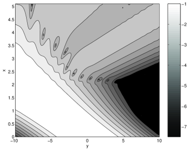
Figure 1: Contour of the $\log_{10}(|u|)$ for the boundary conditions (5). $a=2$, $p=5$, $E/E_{0}=1.216\cdot 10^{-4}$.

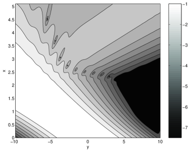
Figure 2: Contour of the $\log_{10}(|u|)$ for the boundary conditions (11). $a=2$, $p=5$, $E/E_{0}=7.875\cdot 10^{-5}$.

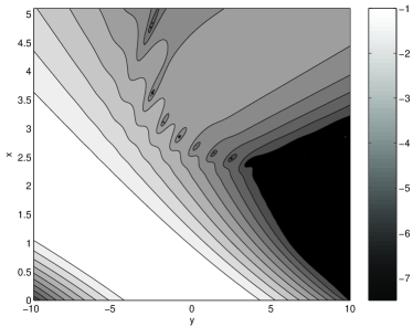
Figure 3: Contour of the $\log_{10}(|u|)$ for the Baskakov-Popov boundary conditions bas-pop . $a=2$, $p=5$, $E/E_{0}=3.251\cdot 10^{-5}$.

The calculations were done with the use of the Crank-Nicolson finite-difference scheme pot with the parameters of the Gaussian beam $a=2$, $p=5$ and $a=1/16$, $p=40$. The results of calculations for the first case with the grid size $1025\times 1025$ are presented in FIG. 1 and FIG. 2. In FIG. 3 are presented the results of calculations with the use of the boundary conditions of Baskakov and Popov bas-pop , which are analytically exact, so this figure shows the effect of the used discretization. In the captions of these figures we present also the values of the relative energy of the reflected waves

$$E/E_{0}=\int^{y_{max}}_{y_{min}}|u(x_{max},y)|^{2}\,dy/\int^{y_{max}}_{y_{min}}|u(0,y)|^{2}\,dy\,.$$

The results of calculations for the narrow Gaussian beam with parameters $a=1/16$, $p=40$, which were done in the domain $[0\leq x\leq 0.15]\times[-2\leq y\leq 2]$, show the following values of the relative energy:

• $3.585\cdot 10^{-5}$, $5.677\cdot 10^{-5}$ and $1.834\cdot 10^{-6}$ for the zeroth order, first order and Baskakov-Popov boundary conditions respectively on the grid $1025\times 1025$;

• $1.066\cdot 10^{-4}$, $2.427\cdot 10^{-4}$ and $1.971\cdot 10^{-5}$ for the zeroth order, first order and Baskakov-Popov boundary conditions respectively on the grid $513\times 513$.

These results confirm that the inverse width of the beam $1/\sqrt{a}$ plays the rôle of the small parameter and show also that for narrow beams the zeroth order boundary conditions can be better than the first order ones, even on the big grid, and more robust with respect to the roughness of the grid.

The dependence of the accuracy of the boundary conditions (12) on the beam width was investigated in some details in kus .

IV Conclusion

In this paper the absorbing boundary conditions (5) and (11) for the variable coefficient Schrödinger type equation (1) were derived by the multiple-scale method. These boundary conditions explicitly take into account the variability of the coefficients and are easy to use. The solution of the Hamilton-Jacobi equation, which is required in these conditions, can be in most cases obtained analytically by the far-field approximations or numerically by the method of the eulerian geometric optics be .

The reported method can be easily generalized to the many-dimensional case.

References

• (1) Babich, V. M., and Buldyrev, V. S. (1972): Asymptotic Methods in Short-Wave Diffraction Problems. Nauka, Moscow [English translation: Springer Series on Wave Phenomena 4. Springer, Berlin et. al., 1991], Zbl. 255.35002
• (2) Engquist, B. and Majda A. Mathematics of Computation, 31, 639, (1977).
• (3) Bender, C. M. and Orszag S. A. Advanced Mathematical Methods for Scientists and Engineers. McGraw-Hill, (1978).
• (4) Shibata, T. Physical Review B, 43, 6760, (1991).
• (5) Kuska, J.-P. Physical Review B, 46, 5000, (1992).
• (6) Baskakov, V.A. and Popov, A.V. Wave Motion, 14, 123, (1991).
• (7) Nayfeh, A.H. Perturbation methods. N.-Y.: John Wiley & Sons, (1973).
• (8) Trofimov, M.Yu. Technical Physics Letters, 31, 400, (2005).
• (9) Maslov, V. P. Russian mathamatical surveys, 42, 43, (1987).
• (10) Potter, D. Computational physics. N.-Y.: John Wiley & Sons, (1973).
• (11) Benamou, J.-D. Comm. Pure Appl. Math., 52, 1443, (1999). Also see INRIA report No. 4628, (2002).