A lower bound for nodal count on discrete and metric graphs

Abstract.

We study the number of nodal domains (maximal connected regions on which a function has constant sign) of the eigenfunctions of Schrödinger operators on graphs. Under certain genericity condition, we show that the number of nodal domains of the $n$-th eigenfunction is bounded below by $n-\ell$, where $\ell$ is the number of links that distinguish the graph from a tree.

Our results apply to operators on both discrete (combinatorial) and metric (quantum) graphs. They complement already known analogues of a result by Courant who proved the upper bound $n$ for the number of nodal domains.

To illustrate that the genericity condition is essential we show that if it is dropped, the nodal count can fall arbitrarily far below the number of the corresponding eigenfunction.

In the appendix we review the proof of the case $\ell=0$ on metric trees which has been obtained by other authors.

1. Introduction

According to a well-know theorem by Sturm, the zeros of the $n$-th eigenfunction of a vibrating string divide the string into $n$ “nodal intervals”. The Courant nodal line theorem carries over one half of Sturm’s theorem to the theory of membranes: Courant proved that the $n$-th eigenfunction cannot have more than $n$ domains. He also provided an example showing that no non-trivial lower bound for the number nodal domains can be hoped for in $\mathbb{R}^{d}$, $d\geq 2$.

But what can be said about the number of nodal domain on graphs? Earliest research on graphs concentrated on Laplace and Schrödinger operators on discrete (combinatorial) graphs. The functions on discrete graphs take values on vertices of the graph and the Schrödinger operator is defined by

$$(H\boldsymbol{\psi})_{u}=-\sum_{v\sim u}\psi_{v}+q_{u}\psi_{u},$$

where the sum is taken over all vertices adjacent to the vertex $u$.

Gantmacher and Krein [13] proved than on a chain graph (a tree with no branching which can be thought of as a discretization of the interval) an analogue of Sturm’s result holds: the $n$-th eigenvector changes sign exactly $n-1$ times. But for non-trivial graphs the situation departs dramatically from its $\mathbb{R}^{d}$ analogue. First of all, Courant’s upper bound does not always hold. There is a correction due to multiplicity of the $n$-th eigenvalue and the upper bound becomes [8] $n+m-1$, where $m$ is the multiplicity. In this paper we discuss another striking difference. If the number of cycles of a graph is not large, the graph behaves “almost” like a string: for a typical eigenvector, there is a lower bound on the number of nodal domains.

To be more precise, let $\ell$ be the minimal number of edges of the graph that distinguish it from a tree (a graph with no loops). In terms of the number of vertices $V$ and the number of edges $E$, the number $\ell$ can be expressed as $\ell=E-V+1$. We show that, for a typical eigenvector, the number of nodal domains is greater or equal to $n-\ell$. In particular, on trees ($\ell=0$) the nodal counting is exact: the $n$-th eigenfunction has exactly $n$ domains. Here by a “typical” eigenvector we mean an eigenvector which corresponds to a simple eigenvalue and which is not zero on any of the vertices. This property is stable with respect to small perturbations of the potential $\{q_{u}\}$.

Another graph model on which the question of nodal domains is well-defined is the so-called quantum or metric graphs. These are graphs with edges parameterized by the distance to a pre-selected start vertex. The functions now live on the edges of the graph and are required to satisfy matching conditions on the vertices of the graph. The Laplacian in this case is the standard 1-dimensional Laplacian. A good review of the history of quantum graphs and some of their applications can be found in [19].

The ideas that the zeros of the eigenfunctions on the metric trees behave similarly to the 1-dimensional case have been around for some time. Al-Obeid, Pokornyi and Pryadiev [1, 23, 22] showed that for a metric tree in a “general position” (which is roughly equivalent to our genericity assumption 2, see Section 3) the number of the nodal domains of $n$-th eigenfunction is equal to $n$. This result was rediscovered by Schapotschnikow [24] who was motivated by the recent interest towards nodal domains in the physics community [4, 15, 14].

Our result on the lower bound extends to the quantum graphs as well. Similarly to the discrete case, we prove that even for graphs with $\ell>0$, $n-\ell$ is a lower bound on the number of nodal domains of the $n$-th eigenfunction.

The article is structured as follows. In Section 2 we explain the models we are considering, formulate our result and review the previous results on the nodal counting on graphs. The case of the metric trees has been treated before in [22, 24]. In the three remaining cases, metric graphs with $\ell>0$, discrete trees and discrete graphs with $\ell>0$, we believe our results to be previously unknown and in Section 3 we provide complete proofs. For completeness, we also include a sketch of the general idea behind the proofs of [22, 24] in the Appendix. Finally, in the last subsection of Section 3 we show that when a graph does not satisfy our genericity conditions, the nodal count can fall arbitrarily far below the number of the corresponding eigenfunction.

2. The main result

2.1. Basic definitions from the graph theory

Let $\mathbb{G}$ be a finite graph. We will denote by $\mathcal{V}$ the set of its vertices and by $\mathcal{E}$ the set of undirected edges of the graph. If there exists an edge connecting two vertices $v_{1}$ and $v_{2}$, we say that the vertices are adjacent and denote it by $v_{1}\sim v_{2}$. We will assume that $\mathbb{G}$ is connected.

Definition 2.1.

A graph $\mathbb{G}$ is connected if for any $v_{1},v_{2}\in\mathcal{V}$ there is a sequence of distinct vertices $u_{1},\ldots u_{n}$ leading from $v_{1}$ to $v_{2}$ ($u_{1}=v_{1}$, $u_{n}=v_{2}$ and $u_{j}\sim u_{j+1}$ for $j=1,\ldots n-1$). A graph $\mathbb{G}$ is a tree if for any $v_{1}$ and $v_{2}$ the sequence of $u_{j}$ connecting them is unique.

The number of edges emanating from a vertex $v$ is called the degree of $v$. Because we only consider connected graphs, there are no vertices of degree 0. If a vertex $v$ has degree 1, we call it a boundary vertex, otherwise we call it internal.

It will sometimes be convenient to talk about directed edges of the graph. Each non-directed edge produces two directed edges going in the opposite directions. These directed edges are reversals of each other. The notation for the reversal of $d$ is $\overline{d}$; the operation of reversal is reflexive: $\overline{\overline{d}}=d$. Directed edges always come in pairs, in other words, there are no edges that are going in one direction only. The set of all directed edges will be denoted by $\mathfrak{E}$. If an edge $d$ emanates from a vertex $v$, we express it by writing $v\prec d$.

The number of vertices is denoted by $|\mathcal{V}|$ and the number of non-directed edges is $|\mathcal{E}|$. Correspondingly, the number of directed edges is $|\mathfrak{E}|=2|\mathcal{E}|$.

Another key definition we will need is the dimension of the cycle space of $\mathbb{G}$.

Definition 2.2.

The dimension $\ell$ of the cycle space of $\mathbb{G}$ is the number of edges that have to be removed from $\mathcal{E}$ (leaving $\mathcal{V}$ as it is) to turn $\mathbb{G}$ into a connected tree.

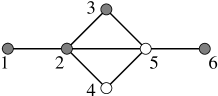
Figure 1. An example of a graph with $\ell=2$. For example, one can cut edges $(2,3)$ and $(4,5)$ to make it a tree. If $\phi$ is positive on shaded vertices and negative on white vertices, the nodal domain count on the graph is 3. On the tree obtained by deleting $(2,3)$ and $(4,5)$ the nodal count would be 5.

Remark 2.3.

An alternative characterization of $\ell$ would be the rank of the fundamental group of $\mathbb{G}$. There is also an explicit expression for $\ell$ in terms of the number of edges and number of vertices of the graph,

(2.1) $$\ell=|\mathcal{E}|-|\mathcal{V}|+1.$$

Obviously, $\ell=0$ if and only if $\mathbb{G}$ is a tree.

2.2. Functions on discrete graphs

The functions on $\mathbb{G}$ are the functions from the vertex set $\mathcal{V}$ to the set of reals, $\boldsymbol{\psi}:\mathcal{V}\to\mathbb{R}$. We only consider finite graphs, therefore the set of all functions $\boldsymbol{\psi}$ can be associated with $\mathbb{R}^{|\mathcal{V}|}$, where $|\mathcal{V}|$ is the number of vertices of the graph.

Given a function $\boldsymbol{\psi}$ on $\mathbb{G}$, we define a positive domain on $\mathbb{G}$ with respect to $\boldsymbol{\psi}$ to be a maximal connected subgraph $S$ of $\mathbb{G}$ such that $\boldsymbol{\psi}$ is positive on the vertices of $S$. Similarly we define the negative domains. Then the nodal domain count $\nu_{\mathbb{G}}(\boldsymbol{\psi})$ is the total number of positive and negative domains on $\mathbb{G}$ with respect to $\boldsymbol{\psi}$, see Fig. 1 for an example. When the choice of the graph is obvious, we will drop the subscript $\mathbb{G}$.

Our interest lies with the nodal domain counts of the eigenvectors of (discrete) Schrödinger operators on graphs. We define the Schrödinger operator with the potential $q:\mathcal{V}\to\mathbb{R}$ by

(2.2) $$(H\boldsymbol{\psi})_{u}=-\sum_{v\sim u}\psi_{v}+q_{u}\psi_{u}.$$

The eigenproblem for the operator $H$ is $H\boldsymbol{\psi}=\lambda\boldsymbol{\psi}$. The operator $H$ has $|\mathcal{V}|$ eigenvalues, which we number in increasing order,

$$\lambda_{1}\leq\lambda_{2}\leq\ldots\leq\lambda_{|\mathcal{V}|}.$$

This induces a numbering of the eigenvectors: $H\boldsymbol{\psi}^{(n)}=\lambda_{n}\boldsymbol{\psi}^{(n)}$. This numbering is well-defined if there are no degeneracies in the spectrum, i.e. $\lambda_{j}\neq\lambda_{k}$ whenever $j\neq k$. By $\nu_{H}(\lambda_{n})$ we denote the nodal domain count of the $n$-th eigenvector $\boldsymbol{\psi}^{(n)}$ of an operator $H$.

2.3. Functions on metric graphs

A metric graph is a pair $(\mathbb{G},\{L_{e}\})$, where $L_{e}$ is the length of the edge $e\in\mathcal{E}$. The lengths of the two directed edges corresponding to $e$ are also equal to $L_{e}$. In particular, $L_{d}=L_{\overline{d}}$.

We would like to consider functions living on the edges of the graph. To do it we identify each directed edge $d$ with the interval $[0,L_{d}]$. This gives us a local variable $x_{d}$ on the edge which can be interpreted geometrically as the distance from the initial vertex. Note that if the edge $\bar{d}$ is the reverse of the edge $d$ then $x_{\bar{d}}$ and $L_{d}-x_{d}$ refer to the same point. Now one can define a function on an edge and, therefore, define a function $\boldsymbol{\psi}$ on the whole graph as a collection of functions $\{\psi_{d}\}_{d\in\mathfrak{E}}$ on all edges of the graph. To ensure that the function is well defined we impose the condition $\psi_{d}(x_{d})=\psi_{\bar{d}}\left(L_{d}-x_{d}\right)$ for all $d\in\mathfrak{E}$. The scalar product of two square integrable functions $\boldsymbol{\psi}$ and $\boldsymbol{\phi}$ is defined as

(2.3) $$\langle\boldsymbol{\psi},\boldsymbol{\phi}\rangle\stackrel{{\scriptstyle\mathrm{def}}}{{=}}\sum_{e\in\mathcal{E}}\int_{0}^{L_{e}}\psi_{e}(x_{e})\overline{\phi_{e}(x_{e})}{\mathrm{d}}x_{e}.$$

This scalar product defines the space $L^{2}(\mathbb{G})$.

To introduce the main object of our study, the nodal domains, on metric graphs we need to define the notion of the metric subgraph of $(\mathbb{G},\{L_{e}\})$.

Definition 2.4.

A metric subgraph of $(\mathbb{G},\{L_{e}\})$ is a metric graph obtainable from $\mathbb{G}$ by (a) cutting some of the edges of $\mathbb{G}$ and thus introducing new boundary vertices, (b) removing some of the edges and (c) removing all vertices of degree 0.

An example of a metric subgraph is shown on Fig. 2. Now, similarly to the discrete case, we can define the nodal count for a real-valued function $\boldsymbol{\phi}$.

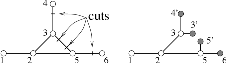
Figure 2. An example of a graph and its metric subgraph. The shaded vertices are the new ones which appeared due to cuts.

A positive (negative) domain with respect to a real-valued function $\boldsymbol{\phi}$ is a maximal connected metric subgraph on whose edges and internal vertices $\boldsymbol{\phi}$ is positive (corresp. negative). The total number of positive and negative domains will be called the nodal count of $\boldsymbol{\phi}$ and denoted by $\nu(\boldsymbol{\phi})$.

We are interested in the nodal counts of the eigenfunctions of the Laplacian $\Delta=-\frac{{\mathrm{d}}^{2}}{{\mathrm{d}}x^{2}}$. As its domain we take the set of continuous functions that belong to the Sobolev space $H^{2}(e)$ on each edge $e$ and satisfy the Kirchhoff condition

(2.4) $$\sum_{d\succ v}\frac{{\mathrm{d}}}{{\mathrm{d}}x}\psi_{d}(0)=0\qquad\mbox{ for all }v\in\mathcal{V}.$$

Note that the sum is taken over all directed edges that originate from the vertex $v$ and the derivative (which depends on the direction of the edge) is taken in the outward direction. The Laplacian can also be defined via the quadratic form

(2.5) $$Q_{\Delta}[\boldsymbol{\psi}]=\sum_{e\in\mathcal{E}}\int_{0}^{L_{e}}|\psi_{e}^{\prime}(x_{e})|^{2}{\mathrm{d}}x_{e}.$$

The domain of this form is the Sobolev space $H^{1}(\mathbb{G})$.

For boundary vertices condition (2.4) reduces to the Neumann condition $\psi^{\prime}_{d}(0)=0$. We also consider other homogeneous conditions on the vertex $v$, of the general form

(2.6) $$\psi^{\prime}_{d}(0)\cos\alpha_{v}=\psi_{d}(0)\sin\alpha_{v},$$

where the Neumann condition corresponds to the choice $\alpha_{d}=0$. The corresponding quadratic form will then change to

(2.7) $$Q_{\Delta}[\boldsymbol{\psi}]=\sum_{e\in\mathcal{E}}\int_{0}^{L_{e}}|\psi_{e}^{\prime}(x_{e})|^{2}{\mathrm{d}}x_{e}+\sum_{v:\deg(v)=1}\psi^{2}(v)\tan\alpha_{v},$$

where the sum is over the boundary vertices and $\psi(v)$ is the value of the function at the vertex $v$.

Our results will also apply to Schrödinger operators $H=\Delta+q(x)$ with a potential $q(x)$ which is continuous on every edge of the graph.

Schrödinger operator $H$, defined in the above fashion, has an infinite discrete spectrum with no accumulation points. As in the discrete case, we number the eigenvalues in the increasing order. We will denote by $\boldsymbol{\psi}^{(n)}$ the eigenvector corresponding to the eigenvalue $\lambda_{n}$.

2.4. Our assumptions and results

Let $\lambda_{n}$ be the $n$-th eigenvalue of the Schrödinger operator $H$ on either discrete or metric graph. Let $\boldsymbol{\psi}^{(n)}$ be the corresponding eigenfunction. We shall make the following assumptions.

Assumption 1.

The eigenvalue $\lambda_{n}$ is simple and the corresponding eigenvector $\boldsymbol{\psi}^{(n)}$ is non-zero on each vertex.

Remark 2.5.

The properties described in the Assumption are generic and stable with respect to a perturbation. Relevant perturbations include changing the potential $\{q_{v}\}$ in the discrete case and changing lengths $\{L_{e}\}$ in the metric case. More precisely, in the finite-dimensional space of all potentials (corresp. lengths) the set $A_{n}$ on which $(\lambda_{n},\boldsymbol{\psi}^{(n)})$ satisfy the Assumption is open and dense unless the graph is a circle (see [11], where this question is discussed for metric graphs). We also mention that on each connected component of the set $A_{n}$ the nodal count of $\boldsymbol{\psi}^{(n)}$ remains the same. Indeed, on discrete graphs the sign of the eigenvector on each vertex must remain unchanged. On metric graphs the zeros cannot pass through the vertices. Moreover zeros cannot undergo a bifurcation (i.e. appear or disappear) — otherwise at the bifurcation point the eigenfunction and its derivative are both zero. By uniqueness theorem for $H\boldsymbol{\psi}=\lambda\boldsymbol{\psi}$, this would mean that $\boldsymbol{\psi}$ is identically zero on the whole edge, contradicting the Assumption.

Now we are ready to state the main theorem which applies to both discrete and metric graphs.

Theorem 2.6.

Let $\lambda_{n}$ and $\boldsymbol{\psi}^{(n)}$ be the $n$-th eigenvalue and the corresponding eigenvector of the Schrödinger operator $H$ on either discrete or metric graph $\mathbb{G}$. If $(\lambda_{n},\boldsymbol{\psi}^{(n)})$ satisfy Assumption 1, then the nodal domain count of $\boldsymbol{\psi}^{(n)}$ is bounded by

(2.8) $$n-\ell\leq\nu(\boldsymbol{\psi}^{(n)})\leq n,$$

where $\ell=|\mathcal{E}|-|\mathcal{V}|+1$ is the dimension of the cycle space of $\mathbb{G}$. In particular, when $\mathbb{G}$ is a tree, $\nu(\boldsymbol{\psi}^{(n)})=n$.

While we state the theorem in the most complete form, we will prove only those parts of it that we believe to be new. The upper bound on the number of nodal domains is a result with a long history going back to Courant [6, 7]. The original proof for domains in $\mathbb{R}^{d}$ was adapted to metric graphs by Gnutzmann, Weber and Smilansky [15], who used the $\mathbb{R}^{d}$ proof from Pleijel [21] who, in turn, cites Herrmann [17] who simplified the original proof of Courant [6].

The history of the discrete version of Courant’s upper bound is more complicated. The question was considered by Colin de Verdière [5], Friedman [12], Duval and Reiner [9], and Davies, Gladwell, Leydold and Stadler [8]. The latter paper contains a good overview of the history of the result and points out various shortcomings in the preceding papers. The point of difficulty was counting the nodal domains if an eigenvalue is degenerate (and therefore there is an eigenvector which is zero on some vertices). As shown in [8], the upper bound is $n+m-1$, where $m$ is the multiplicity of the eigenvalue. In our case, Assumption 1, which is essential for the lower bound (see Section 3.4), also simplifies the upper bound.

The lower bound for the nodal domains on metric trees (i.e. the $\ell=0$ case) was shown by Al-Obeid, Pokornyi and Pryadiev [1, 23, 22] and by Schapotschnikow [24]. For completeness, we give a sketch of the proof of this case in the Appendix.

Finally, the results on the lower bound for discrete graphs (both $\ell=0$ and $\ell>0$ cases) and for metric graphs with $\ell>0$ are new and will be proved in this paper.

Note added in proof: It has been brought to the author’s attention by J. Leydold that the lower bound for discrete trees has been also obtained by Bıyıkoğlu [3] as a corollary of a result of Fiedler [10].

3. Proofs

We will apply induction on $\ell$ to deduce the statement for metric graphs. The proofs for the discrete case follow the same ideas but differ in some significant detail.

First, however, we discuss an important consequence of Remark 2.5: it is sufficient to prove statements on nodal counts under the following stronger Assumption.

Assumption 2.

Assumption 1 is satisfied for all eigenpairs $(\lambda_{k},\boldsymbol{\psi}^{(k)})$ with $k\leq n$.

Indeed, if only Assumption 1 is satisfied but Assumption 2 is not, we can perturb the problem so that (a) the nodal count of the $n$-th eigenfunction $\boldsymbol{\psi}^{(n)}$ does not change and (b) Assumption 1 becomes satisfied for all $k\leq n$. Then, anything proved about the nodal domains of $\boldsymbol{\psi}^{(n)}$ in the perturbed problem (which satisfies Assumption 2) will still be valid for the unperturbed one.

In our proofs we use the classical ideas of mini-max characterization of the eigenvalues. Let $H$ be a self-adjoint operator with domain $\mathcal{D}$. Assume the spectrum of $H$ is discrete and bounded from below. Let $Q_{H}[\boldsymbol{\psi}]=(\boldsymbol{\psi},H\boldsymbol{\psi})$ be the corresponding quadratic form. Then the eigenvalues of $H$ can be obtained as

(3.1) $$\lambda_{k+1}=\max_{f_{1},\ldots,f_{k}\in\mathcal{D}^{\prime}}\ \min_{\boldsymbol{\psi}\in\mathcal{D},\ f_{j}(\boldsymbol{\psi})=0}\frac{Q_{H}[\boldsymbol{\psi}]}{(\boldsymbol{\psi},\boldsymbol{\psi})},$$

where the maximum is taken over all linear functionals over $\mathcal{D}$.

We will need the following classical theorem (see, e.g., [7, Chapter VI] or [16, Chapter II])

Theorem 3.1 (Rayleigh’s Theorem of Constraint).

Let $H$ be a self-adjoint operator defined on $\mathcal{D}$. If $H$ is restricted to a subdomain $\mathcal{D}_{R}=\{\boldsymbol{\psi}\in\mathcal{D}:g(\boldsymbol{\psi})=0\}$, where $g\in\mathcal{D}^{\prime}$, then the eigenvalues $\mu_{n}$ of the restricted operator satisfy

$$\lambda_{n}\leq\mu_{n}\leq\lambda_{n+1},$$

where $\lambda_{n}$ are the eigenvalues of the unrestricted operator.

3.1. Metric graphs ($\ell>0$)

We will derive the lower bound for graphs with cycles by cutting the cycles and using the lower bound for trees.

Proof of Theorem 2.6 for metric graphs ($\ell>0$).

We are given an eigenpair $(\lambda_{n},\boldsymbol{\psi}^{(n)})$. Assume that cutting the edges $e_{1},\ldots,e_{\ell}$ turns the graph $\mathbb{G}$ into a tree. We cut each of these edges at a point $x_{j}\in e_{j}$ such that $\boldsymbol{\psi}^{(n)}(x_{j})\neq 0$. We thus obtain a tree with $|\mathcal{E}(\mathbb{G})|+\ell$ edges and $|\mathcal{V}(\mathbb{G})|+2\ell$ vertices. Denote this tree by $\mathbb{T}$. There is a natural mapping from the functions on the graph $\mathbb{G}$ to the functions on the tree $\mathbb{T}$. In particular, we can think of $\boldsymbol{\psi}^{(n)}$ as living on the tree.

We would like to consider the same eigenproblem $H\boldsymbol{\psi}=\mu\boldsymbol{\psi}$ on the tree now. The vertex conditions on the vertices common to $\mathbb{T}$ and $\mathbb{G}$ will be inherited from the eigenproblem on $\mathbb{G}$. But we need to choose the boundary conditions at the $2\ell$ new vertices. Each cut-point $x_{j}$ gives rise to two vertices, which we will denote by $u_{j+}$ and $u_{j-}$. Define

$$a_{j+}=\frac{\frac{d}{dx}\boldsymbol{\psi}^{(n)}(u_{j+})}{\boldsymbol{\psi}^{(n)}(u_{j+})},\qquad a_{j-}=\frac{\frac{d}{dx}\boldsymbol{\psi}^{(n)}(u_{j-})}{\boldsymbol{\psi}^{(n)}(u_{j-})},\qquad j=1,\ldots,\ell,$$

where the derivatives are taken in the inward direction on the corresponding edges of $\mathbb{T}$. Since $\boldsymbol{\psi}^{(n)}$, as an eigenfunction, was continuously differentiable and $\boldsymbol{\psi}^{(n)}(u_{j+})=\boldsymbol{\psi}^{(n)}(u_{j-})$, we have $a_{j+}=-a_{j-}$.

Now we set the boundary conditions on the new vertices of $\mathbb{T}$ to be

$$\frac{d}{dx}\psi(u_{j+})=a_{j+}\psi(u_{j+}),\qquad\frac{d}{dx}\psi(u_{j-})=a_{j-}\psi(u_{j-}),\qquad j=1,\ldots,\ell,$$

where the derivatives, as before, are taken inwards. By definition of the coefficients $a_{j\pm}$, the function $\boldsymbol{\psi}^{(n)}$ satisfies the above boundary conditions. It also satisfies the equation $H\boldsymbol{\psi}=\mu\boldsymbol{\psi}$ and the vertex conditions throughout the rest of the tree. Thus, $\boldsymbol{\psi}^{(n)}$ is also an eigenfunction on $\mathbb{T}$ and $\lambda_{n}$ is the corresponding eigenvalue. If we denote the ordered eigenvalues of $\mathbb{T}$ by $\mu_{k}$, then $\lambda_{n}=\mu_{m}$ for some $m$. It is important to note that $m$ is in general different from $n$. We will now show that $m\geq n$.

Denote by $Q_{\mathbb{G}}[\boldsymbol{\psi}]$ the quadratic form corresponding to the eigenvalue problem on $\mathbb{G}$; its domain we denote by $\mathcal{H}_{\mathbb{G}}$. Similarly we define $Q_{\mathbb{T}}[\boldsymbol{\psi}]$ and $\mathcal{H}_{\mathbb{T}}$. As we mentioned earlier, there is a natural embedding of $\mathcal{H}_{\mathbb{G}}$ into $\mathcal{H}_{\mathbb{T}}$. Moreover, we can say that

$$\mathcal{H}_{\mathbb{G}}=\left\{\boldsymbol{\psi}\in\mathcal{H}_{\mathbb{T}}:\psi(u_{j+})=\psi(u_{j-}),j=1,\ldots,\ell\right\}.$$

We also note that, formally,

$$Q_{\mathbb{T}}[\boldsymbol{\psi}]=Q_{\mathbb{G}}[\boldsymbol{\psi}]+\sum_{j=1}^{\ell}\left(a_{j+}\psi^{2}(u_{j+})+a_{j-}\psi^{2}(u_{j-})\right).$$

If $\boldsymbol{\psi}\in\mathcal{H}_{\mathbb{G}}$ then $\psi(u_{j+})=\psi(u_{j-})$ and $a_{j+}=-a_{j-}$ result in the cancellation of the sum on the right-hand side. This means that on $\mathcal{H}_{\mathbb{G}}$, $Q_{\mathbb{T}}[\boldsymbol{\psi}]=Q_{\mathbb{G}}[\boldsymbol{\psi}]$.

Now we employ the minimax formulation for the eigenvalues $\lambda_{k}$ on $\mathbb{G}$,

$$\lambda_{k+1}=\max_{\phi_{1},\ldots,\phi_{k}\in\mathcal{H}_{\mathbb{G}}}\min_{\stackrel{{\scriptstyle\boldsymbol{\psi}\in\mathcal{H}_{\mathbb{G}}}}{{\|\boldsymbol{\psi}\|=1,\ \boldsymbol{\psi}\perp\phi_{i}}}}Q_{\mathbb{G}}[\boldsymbol{\psi}]=\max_{\phi_{1},\ldots,\phi_{k}\in\mathcal{H}_{\mathbb{G}}}\min_{\stackrel{{\scriptstyle\boldsymbol{\psi}\in\mathcal{H}_{\mathbb{G}}}}{{\|\boldsymbol{\psi}\|=1,\ \boldsymbol{\psi}\perp\phi_{i}}}}Q_{\mathbb{T}}[\boldsymbol{\psi}],$$

Comparing it with the corresponding formula for the eigenvalues on $\mathbb{T}$

$$\mu_{k+1}=\max_{\phi_{1},\ldots,\phi_{k}\in\mathcal{H}_{\mathbb{T}}}\min_{\stackrel{{\scriptstyle\boldsymbol{\psi}\in\mathcal{H}_{\mathbb{T}}}}{{\|\boldsymbol{\psi}\|=1,\ \boldsymbol{\psi}\perp\phi_{i}}}}Q_{\mathbb{T}}[\boldsymbol{\psi}],$$

we see that the eigenvalues $\lambda_{k}$ correspond to the same minimax problem as $\mu_{k}$ but with $\ell$ additional constraints $\psi(u_{j+})=\psi(u_{j-})$. By Rayleigh’s theorem we conclude that $\mu_{k}\leq\lambda_{k}$ for any $k$. Therefore, if $\lambda_{n}=\mu_{m}$ for some $n$ and $m$, they must satisfy $m\geq n$.

To finish the proof we need to count the number of nodal domains on $\mathbb{G}$ and on $\mathbb{T}$ with respect to $\boldsymbol{\psi}^{(n)}$. When we cut an edge of $\mathbb{G}$, we increase the number of nodal domains by at most one. Therefore,

$$\nu_{\mathbb{T}}(\boldsymbol{\psi})\leq\nu_{\mathbb{G}}(\boldsymbol{\psi})+\ell.$$

On the other hand, we know that the nodal counting on the tree is exact, and, since $\boldsymbol{\psi}^{(n)}$ is the $m$-th eigenvector on $\mathbb{T}$,

$$\nu_{\mathbb{T}}(\boldsymbol{\psi}^{(n)})=m\geq n.$$

Combining the above inequalities we obtain the desired bound

$$\nu_{\mathbb{G}}(\boldsymbol{\psi}^{(n)})\geq n-\ell.$$

To conclude the proof we acknowledge that we implicitly assumed that the tree $\mathbb{T}$ satisfies Assumption 1, more precisely, that the eigenvalue $\mu_{r}$ is simple. To justify it, we observe that, if this is not the case, a small perturbation in the lengths of the edges will force $\mathbb{T}$ to become generic but will not affect the properties of the eigenvectors of $\mathbb{G}$. ∎

3.2. Discrete trees ($\ell=0$)

Take an arbitrary vertex of $\mathbb{T}$ and designate it as root, denoted $r$. The tree with a root induces partial ordering on the vertices $\mathcal{V}$: we say that $v_{1}<v_{2}$ if the unique path connecting $v_{1}$ with $r$ passes through $v_{2}$ (see Definition 2.1). We denote by $v_{1}\prec v_{2}$ the situation when $v_{1}<v_{2}$ and $v_{1}\sim v_{2}$.

In the above ordering the root is higher than any other vertex. Since $\mathbb{T}$ is a tree, for each vertex $v$, other than the root, there is a unique $u$ such that $v\prec u$. Given a non-vanishing $\boldsymbol{\psi}$ we introduce the new variables $R_{v}=\psi_{u}/\psi_{v}$, where $v\prec u$. Variables $R_{v}$ are sometimes called Riccati variables [20].

The eigenvalue condition $H\boldsymbol{\psi}=\lambda\boldsymbol{\psi}$ can now be written as

(3.2) $$-\psi_{u}-\sum_{w\prec v}\psi_{w}+q_{v}\psi_{v}=\lambda\psi_{v},$$

and, after dividing by $\psi_{v}$,

(3.3) $$R_{v}=q_{v}-\lambda-\sum_{w\prec v}\frac{1}{R_{w}}.$$

If $v$ is the root, condition (3.2) takes the form

$$-\sum_{w\prec r}\psi_{w}+q_{r}\psi_{r}=\lambda\psi_{r}.$$

Therefore, if we define

$$R_{r}\equiv q_{r}-\lambda-\sum_{w\sim r}\frac{1}{R_{w}},$$

then the zeros of $R_{r}$ in terms of $\lambda$ are the eigenvalues of $H$. Whenever $R_{r}(\lambda)=0$, the values of $R_{v}$, $v\neq r$, uniquely specify the corresponding eigenvector $\boldsymbol{\psi}$ of $H$, and vice versa.

Equation (3.3) provides a recursive algorithm for calculating $R_{v}$, in order of increasing $v$. Thus one gets a closed formula for $R_{v}$ in terms of $q_{u}$, $u\leq v$ and $\lambda$. This is best illustrated by an example.

Figure 3. An example of a tree graph with $5$ being the root vertex.

Example 3.2.

For the tree shown in Fig. 3 the eigenvalue condition in terms of Riccati variables reads

(3.4) $$R_{1} = q_{1}-\lambda,$$

(3.5) $$R_{2} = q_{2}-\lambda,$$

(3.6) $$R_{3} = q_{3}-\lambda,$$

(3.7) $$R_{4} = q_{4}-\lambda-\frac{1}{R_{1}}-\frac{1}{R_{2}},$$

(3.8) $$0 = q_{5}-\lambda-\frac{1}{R_{3}}-\frac{1}{R_{4}}\equiv R_{5}.$$

By substituting lines (3.4) and (3.5) into equation (3.7), and then lines (3.6) and (3.7) into equation (3.8), one obtains an eigenvalue condition for $H$.

Denote by $P_{v}$ the set of all poles of $R_{v}$ with respect to $\lambda$ and by $Z_{v}$ the set of all zeros of $R_{v}$; these sets are finite. We define $N_{v}^{<}$ to be the number of negative values among $R_{u}$ with $u<v$; we similarly define $N_{v}^{\leq}$:

(3.9) $$N_{v}^{<}=\Big{|}\{u<v:R_{u}<0\}\Big{|},\qquad N_{v}^{\leq}=\Big{|}\{u\leq v:R_{u}<0\}\Big{|}.$$

The above numbers are not defined whenever one of $R_{u}$ has a zero or a pole. The following lemma, listing properties of the Riccati variables, their poles and zeros, amounts to the proof of Theorem 2.6 when $\mathbb{G}$ is a tree and $q$ is generic.

Lemma 3.3.

Assume that, for each $v$, the sets $Z_{w}$ with $w\prec v$ are pairwise disjoint for all $v$. Then

1. $P_{v}=\bigcup_{w\prec v}Z_{w}$

2. For every $p\in P_{v}$, $lim_{\lambda\to p-0}R_{v}=-\infty$ and $lim_{\lambda\to p+0}R_{v}=+\infty$. Also, $lim_{\lambda\to-\infty}R_{v}=+\infty$ and $lim_{\lambda\to\infty}R_{v}=-\infty$. Outside the poles, $R_{v}$ is continuous and monotonically decreasing as a function of $\lambda$.

3. There is exactly one zero of $R_{v}$ strictly between each pair of consecutive points from the set $\{-\infty\}\cup\{\infty\}\cup P_{v}$.

4. Between each pair of consecutive points from $\{-\infty\}\cup\{\infty\}\cup Z_{v}$, the number $N_{v}^{\leq}$ (where defined) remains constant. When a zero of $R_{v}$ is crossed, $N_{v}^{\leq}$ increases by one.

5. Between each pair of consecutive points from $\{-\infty\}\cup\{\infty\}\cup P_{v}$, the number $N_{v}^{<}$ (where defined) remains constant. When a pole of $R_{v}$ is crossed, $N_{v}^{<}$ increases by one.

6. When $\lambda=\lambda_{n}$ is an eigenvalue of $H$, the number of the nodal domains of $\boldsymbol{\psi}^{(n)}$ is given by

   (3.10) $$\nu(\lambda_{n})=N_{r}^{<}+1.$$

Proof.

Part 1 follows directly from equation (3.3).

Part 2 follows from (3.3) by induction over increasing $v$.

Part 3 follows from part 2: between each pair of consecutive points from $\{-\infty\}\cup\{\infty\}\cup P_{v}$, the function $R_{v}$ decreases from $+\infty$ to $-\infty$.

Parts 4 and 5 are linked together in an induction over increasing $v$. The induction is initialized by $N_{v}^{\leq}$ for minimal $v$ (i.e. there is no $w$ with $w<v$). In this case, $R_{v}=q_{v}-\lambda$, therefore $N_{v}^{\leq}=0$ to the left of $\lambda=q_{v}$ and $N_{v}^{\leq}=1$ to the right of $\lambda=q_{v}$.

The inductive step starts with part 5. For a vertex $v$, let both statements be verified for all $w$, $w<v$. The statement for $N_{v}^{<}$ is obtained immediately from the duality between the zeros and the poles (part 1). Note that the assumption of the lemma implies that only one of $N_{w}^{\leq}$ with $w\prec v$ can increase when $\lambda$ crosses a pole of $R_{v}$.

To obtain the statement for $N_{v}^{\leq}$ consider two consequent poles and two consequent zeros of $R_{v}$, interlacing as follows

$$p_{1}<z_{1}<p_{2}<z_{2}.$$

Then $R_{v}$ is positive for $\lambda\in(p_{1},z_{1})$ (by part 2), therefore, on this interval $N_{v}^{\leq}=N_{v}^{<}$. When $z_{1}$ is crossed, $N_{v}^{\leq}$ increases by one since $R_{v}$ becomes negative: $N_{v}^{\leq}=N_{v}^{<}+1\equiv C$. On the other hand, when $p_{2}$ is crossed, $N_{v}^{\leq}$ and $N_{v}^{<}$ become equal again since $R_{v}>0$. However, $N_{v}^{<}$ has increased by one (by the induction hypothesis) and therefore $N_{v}^{\leq}$ is still equal to $C$. The above is obviously valid even if $p_{1}=-\infty$ or/and $z_{2}=+\infty$.

Finally, to show part 6 we observe that $N_{r}^{<}$ is the number of negative Riccati variables throughout the tree. If $R_{v}<0$ then the signs of $\psi_{v}$ and $\psi_{u}$ (where $u$ is the unique vertex satisfying $v\prec u$) are different, i.e. the edge $(u,v)$ is a boundary between a positive and a negative domain. Removing all boundary edges separates the tree into subtrees corresponding to the positive/negative domains. But removing $N_{r}^{<}$ edges from a tree breaks it into $N_{r}^{<}+1$ disconnected components, therefore the number of domains on a tree is equal to $N_{r}^{<}+1$. ∎

Proof of Theorem 2.6 for discrete trees ($\ell=0$).

The condition of Lemma 3.3 is satisfied due to the genericity assumption. Indeed, if there are $v$, $w_{1}$ and $w_{2}$ such that $w_{1}\prec v$, $w_{2}\prec v$ and $\lambda\in Z_{w_{1}}\cap Z_{w_{2}}$ then one can construct an eigenvector with eigenvalue $\lambda$ and with $\psi_{v}=0$.

Since the sets $Z_{v}$ are finite, $N_{r}^{<}$ must become zero when $\lambda\to-\infty$. Consequently, $N_{r}^{<}$ is zero between $-\infty$ and the first pole of $R_{r}$. Denote by $p_{n}$ the $n$-th pole of $R_{r}$. By part 3 of the lemma, the first eigenvalue $\lambda_{1}$ of $H$ lies in the interval $(\infty,p_{1})$, on which $N_{r}^{<}$ is zero. By (3.10) we thus have $\nu(\lambda_{1})=1$. Further, $\lambda_{2}$ lies in the interval $(p_{1},p_{2})$. By part 5 of the lemma, $N_{r}^{<}=1$ on this interval, giving $\nu(\lambda_{2})=2$. Equality for other $\lambda_{n}$ follows similarly. ∎

3.3. Discrete graphs ($\ell>0$)

In this case $H$ is a matrix and the quadratic form is

(3.11) $$Q_{\mathbb{G}}[\boldsymbol{\psi}]=Q_{H}[\boldsymbol{\psi}]=\sum_{j,k=1}^{|\mathcal{V}|}H_{jk}\psi_{j}\psi_{k},$$

where

$$H_{jk}=\begin{cases}-1,&j\sim k,\\ q_{j},&j=k,\\ 0,&\mbox{otherwise}.\end{cases}$$

Proof of Theorem 2.6 for discrete graphs ($\ell>0$).

We will prove the result by induction. The initial inductive step $\ell=0$ is already proven in Section 3.2.

Assume, without loss of generality, that we can delete the edge $(1,2)$ of the graph $\mathbb{G}$ without disconnecting it. We will denote thus obtained graph by ${\Gamma}$. Note that $\mathcal{V}(\mathbb{G})=\mathcal{V}({\Gamma})$. Let $\boldsymbol{\phi}$ be an eigenvector of $H_{\mathbb{G}}$ with eigenvalue $\lambda_{n}$. We would like to prove that $\nu_{\mathbb{G}}(\boldsymbol{\phi})\geq n-l$.

Set $\alpha=\phi_{2}/\phi_{1}$ and define the potential $p$ on ${\Gamma}$ by

$$p_{j}=\begin{cases}q_{1}-\alpha,&j=1,\\ q_{2}-1/\alpha,&j=2,\\ q_{j},&j\neq 1,2.\end{cases}$$

With the aid of potential $p$ we define the operator $H_{\Gamma}$ in the usual way, see equation (2.2). It is easy to see that, due to our choice of potential $p$, the vector $\boldsymbol{\phi}$ is an eigenvector of $H_{\Gamma}$. For example,

$$\left(H_{\Gamma}\boldsymbol{\phi}\right)_{1}=-\sum_{j\sim 1}\phi_{j}+(q_{1}-\alpha)\phi_{1}=-\sum_{j\sim 1}\phi_{j}-\phi_{2}+q_{1}\phi_{1}=\left(H_{\mathbb{G}}\phi\right)_{1}=\lambda_{n}\phi_{1},$$

where the adjacency is taken with respect to the graph ${\Gamma}$.

The eigenvalue corresponding to $\boldsymbol{\phi}$ remains unchanged. However, in the spectrum $\{\mu_{j}\}_{j=1}^{|\mathcal{V}|}$ of $H_{\Gamma}$, this eigenvalue may occupy a position other than the $n$-th. We denote by $m$ the new position of $\lambda_{n}$: $\mu_{m}=\lambda_{n}$.

Now consider the quadratic form associated with $H_{\Gamma}$. Consulting (3.11) we conclude

(3.12) $$Q_{\Gamma}[\boldsymbol{\psi}]=Q_{\mathbb{G}}[\boldsymbol{\psi}]+2\psi_{1}\psi_{2}-\alpha\psi_{1}^{2}-\alpha^{-1}\psi_{2}^{2}.$$

Consider first the case $\alpha>0$. We write $Q_{\Gamma}[\boldsymbol{\psi}]$ in the form

$$Q_{\Gamma}[\boldsymbol{\psi}]=Q_{\mathbb{G}}[\boldsymbol{\psi}]-(\alpha^{1/2}\psi_{1}-\alpha^{-1/2}\psi_{2})^{2}\leq Q_{\mathbb{G}}[\boldsymbol{\psi}].$$

From here and equation (3.1) we immediately conclude that $\mu_{j}\leq\lambda_{j}$. Therefore, $\mu_{m}=\lambda_{n}$ implies $m\geq n$.

From the inductive hypothesis we know that $\nu_{\Gamma}[\boldsymbol{\phi}]\geq m-(l-1)$. But the number of nodal domains of $\boldsymbol{\phi}$ with respect to ${\Gamma}$ is either the same or one more than the number with respect to $\mathbb{G}$: $\alpha>0$, therefore $\phi_{1}$ and $\phi_{2}$ are of the same sign and we may have cut one domain in two by deleting the edge $(1,2)$. In particular, $\nu_{\Gamma}[\boldsymbol{\phi}]\leq\nu_{\mathbb{G}}[\boldsymbol{\phi}]+1$. Eliminating $\nu_{\Gamma}[\boldsymbol{\phi}]$, we obtain $\nu_{\mathbb{G}}[\boldsymbol{\phi}]+1\geq m-(l-1)$, which is the sought conclusion.

In the case $\alpha<0$ the quadratic form on ${\Gamma}$ can be written as

(3.13) $$Q_{\Gamma}[\boldsymbol{\psi}]=Q_{\mathbb{G}}[\boldsymbol{\psi}]+(\beta^{1/2}\psi_{1}+\beta^{-1/2}\psi_{2})^{2},$$

where $\beta=-\alpha$. Consider the subspace

$$\mathcal{D}_{R}=\{\boldsymbol{\psi}\in\mathbb{R}^{|\mathcal{V}|}:\beta^{1/2}\psi_{1}+\beta^{-1/2}\psi_{2}=0\}.$$

The restrictions of $H_{\mathbb{G}}$ and $H_{\Gamma}$ to this subspace coincide, as can be seen from (3.13). Therefore we can apply Theorem 3.1 twice, obtaining

$$\lambda_{j-1}\leq\rho_{j-1}\leq\lambda_{j}\qquad\mu_{j-1}\leq\rho_{j-1}\leq\mu_{j},$$

where $\rho_{j}$ are the eigenvalues of the restricted operator. In particular, we conclude that $\mu_{j-1}\leq\lambda_{j}$. Since $\lambda$-spectrum is non-degenerate, $\mu_{j-1}<\lambda_{j+1}$, therefore $\mu_{m}=\lambda_{n}$ implies $m\geq n-1$.

On the other hand, the number of nodal domains with respect to ${\Gamma}$ is the same as with respect to $\mathbb{G}$: since $\alpha=\phi_{2}/\phi_{1}<0$, we have cut an edge between two domains. Using the inductive hypothesis we conclude that

$$\nu_{\mathbb{G}}(\boldsymbol{\phi})=\nu_{\Gamma}(\boldsymbol{\phi})\geq m-(l-1)\geq n-1-(l-1)=n-l.$$

We finish the proof with a remark similar to the final statement of the proof for metric graphs. If the new graph ${\Gamma}$ happens not to satisfy Assumption 1, a small perturbation in $q$ will force ${\Gamma}$ to become generic but will not affect the properties of the eigenvectors of $\mathbb{G}$. ∎

3.4. Low nodal count in a non-generic case

In this section we show that the genericity assumption (Assumption 1) is essential for the existence of the lower bound. We shall construct an example in which the assumption is violated and the nodal count becomes very low. The construction is based on the fact that an eigenfunction of a graph (as opposed to a connected domain in $\mathbb{R}^{d}$) may be identically zero on a large set.

We consider a metric star graph, which is a tree with $N$ edges all connected to a single vertex. For Dirichlet boundary conditions one can show [18] that $k^{2}$ is an eigenvalue of the graph if

(3.14) $$\sum_{j=1}^{N}\cot kL_{j}=0.$$

To obtain all eigenvalues of the star graph, one needs to add to the solutions of (3.14) the points which are “multiple” poles of the left-hand side of (3.14). More precisely, if a given $k$ is a pole for $m$ cotangents at the same time, then $k^{2}$ is an eigenvalue of multiplicity $m-1$. Those eigenvalues that are not poles (but zeros) of the left-hand side of (3.14) interlace the poles: between each pair of consecutive poles (coming from different cotangents) there is exactly one zero.

Now we choose the lengths $L_{j}$ to exploit the above features. Let $L_{1}=1$, $L_{2}=1/m$ for some $m\in\mathbb{N}$, and the remaining lengths be irrational pairwise incommensurate numbers slightly greater than 1. By construction, $k=m\pi$ is a pole for $\cot(kL_{1})$ and $\cot(kL_{2})$. The corresponding eigenfunction is a sine-wave on the edges $1$ and $2$ and is zero on the other edges. It is easy to see that it has $m+1$ nodal domains. On the other hand, counting the poles of (3.14), one can deduce that there are $(m-1)(N-1)+1$ eigenvalues preceding $(m\pi)^{2}$. Thus, we have constructed an eigenfunction which is very high in the spectrum but has low number of nodal domains.

A similar construction is possible for discrete graphs as well.

Appendix A Ideas behind the proof for metric trees ($\ell=0$)

In this section we give an informal overview of the proof of (2.8) on a metric tree ($\ell=0$). For detailed and rigorous proofs we refer the reader to [23, 22, 24].

Let $(\lambda_{n},\boldsymbol{\psi}^{(n)})$ be an eigenpair for a tree $\mathbb{T}$ satisfying Assumption 2. Choose an arbitrary boundary vertex of the tree $\mathbb{T}$ and call it the root $r$. We can now orient all edges of the tree towards the root (well-defined because it is a tree) and will be taking derivatives in this direction. For each non-root vertex $v$ there is only one adjacent edge that is directed away from it. We call it the outgoing edge of the vertex $v$. The other adjacent edges are correspondingly incoming. An incoming subtree of vertex $v$ is defined recursively as the union of an incoming edge $(u,v)$ with all incoming subtrees of the vertex $u$, see Fig. 4.

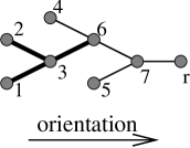
Figure 4. An example of a tree with root $r$. If $v$ is vertex 6 then it has two incoming subtrees, one consisting of edges $(1,3)$, $(2,3)$ and $(3,6)$ (highlighted in thicker lines) and the other consisting of only one edge $(4,6)$. The outgoing edge of $v$ is the edge $(6,7)$.

If we drop the boundary condition at the root, then for any $\lambda\leq\lambda_{n}$ there is a solution $\boldsymbol{\phi}(\lambda,x)$ which solves the equation $H\boldsymbol{\phi}=\lambda\boldsymbol{\phi}$ and satisfies all remaining vertex conditions. This solution is unique up to a multiplicative constant.

The function $\boldsymbol{\phi}$ can be constructed recursively. We fix $\lambda$ and initialize the recursion by solving the equation $H\boldsymbol{\phi}=\lambda\boldsymbol{\phi}$ on the outgoing edge of each non-root boundary vertex and imposing the boundary condition corresponding to this vertex.

Now let $v$ be a vertex such that the equation is solved on each incoming subtree $\mathbb{T}^{v}_{j}$. We denote these solutions (which are defined up to a multiplicative constant) by $C_{j}\phi_{j}(x)$. We would like to match these solutions and to extend them to the outgoing edge of $v$.

Denoting the solution of the outgoing edge by $\phi_{v}(x)$ we write out the matching conditions at the vertex $v$,

$$\phi_{v}(v) =C_{1}\phi_{1}(v)=C_{2}\phi_{2}(v)=\ldots$$

$$\phi_{v}^{\prime}(v) =C_{1}\phi_{1}^{\prime}(v)+C_{2}\phi_{2}^{\prime}(v)+\ldots$$

Suppose that all of the functions $\phi_{j}(x)$ assume non-zero values on the vertex $v$. Then the condition on $\phi_{v}(x)$ takes the form

$$\phi_{v}^{\prime}(v)=\phi_{v}(v)\left(\frac{\phi_{1}^{\prime}(v)}{\phi_{1}(v)}+\frac{\phi_{2}^{\prime}(v)}{\phi_{2}(v)}+\ldots\right).$$

It is now clear that $\phi_{v}$, as a solution of $H\boldsymbol{\phi}=\lambda\boldsymbol{\phi}$ satisfying this condition, is also defined up to a multiplicative constant, $C_{v}$. The continuity condition now fixes the constants $C_{j}$ to be $C_{v}\phi_{v}(v)/\phi_{j}(v)$. Thus we obtain the solution on the union of subtrees $\mathbb{T}^{v}_{j}$ and the outgoing edge of $v$. This union is in turn an incoming subtree for another vertex (or the root).

In the case when one of $\phi_{j}(x)$ is zero on the vertex $v$ (without loss of generality we take $\phi_{1}(v)=0$), the condition on $\phi_{v}$ takes the form $\phi_{v}(v)=0$. The solution $\phi_{v}$ is again defined up to a multiplicative constant $C_{v}$. The values of the other constants are now given by $C_{1}=C_{v}\phi_{v}^{\prime}(v)/\phi_{1}^{\prime}(v)$ and $C_{j}=0$ when $j>1$. Again the solution on the union of subtrees $\mathbb{T}^{v}_{j}$ and the outgoing edge of $v$ is obtained up to a constant.

Finally, if more than one of $\phi_{j}(x)$ is zero on the vertex $v$ (without loss of generality, $\phi_{1}(v)=\phi_{2}(v)=0$), one can take $C_{j}=0$ for all $j>2$, find non-zero $C_{1}$ and $C_{2}$ such that $C_{1}\phi^{\prime}_{1}(v)+C_{2}\phi^{\prime}_{2}(v)=0$ and extend the function by zero on the rest of the tree. This function will satisfy the Kirchhoff condition at $v$ and also all other vertex conditions. Thus it is an eigenfunction and, moreover, it is equal to zero at an inner vertex. This contradicts our assumptions.

We have now constructed a function $\boldsymbol{\phi}(\lambda,x)$ which coincides with the eigenfunction of the tree whenever it satisfies the boundary condition at the root. To count the nodal domains we need to understand the behavior of zeros of $\boldsymbol{\phi}$ as we change $\lambda$. In order to do that we consider the function $R(\lambda,x)=\boldsymbol{\phi}^{\prime}(\lambda,x)/\boldsymbol{\phi}(\lambda,x)$ where the derivative is taken with respect to $x$ in the direction towards the root. If $x$ is a zero of $\boldsymbol{\phi}$, it becomes a pole of $R(\lambda,x)$. From the definition of $R(\lambda,x)$ we see that $R(\lambda,x-0)=-\infty$ and $R(\lambda,x+0)=\infty$. Differentiating $R(\lambda,x)$ with respect to $x$ and using the equation $-\boldsymbol{\phi}^{\prime\prime}+q(x)\boldsymbol{\phi}=\lambda\boldsymbol{\phi}$, we see that $R(\lambda,x)$ satisfies

$$\frac{d}{dx}R=q(x)-\lambda-R^{2},$$

a Riccati-type equation. Conditions (2.6) on the boundary vertices in terms of $R(\lambda,x)$ take the form $R(\lambda,v)=\tan(\alpha_{v})\in\mathbb{R}^{1}\cup\{\infty\}$. The matching conditions on the internal vertices imply that the value of $R(\lambda,v)$ on the outgoing edge is equal to the sum of the values of $R(\lambda,v)$ on the incoming edges (in general, $R$ is not continuous on internal vertices).

Now let $\lambda_{2}>\lambda_{1}$ and $R(\lambda_{2},x_{0})=R(\lambda_{1},x_{0})$. Then $R^{\prime}(\lambda_{2},x)<R^{\prime}(\lambda_{1},x)$ and therefore, on some interval $(x_{0},x_{0}+\epsilon)$, we have $R(\lambda_{2},x)<R(\lambda_{1},x)$. Moreover, once $R(\lambda_{2},x)\leq R(\lambda_{1},x)$, we have $R(\lambda_{2},y)\leq R(\lambda_{1},y)$ for all $y>x$ provided both functions do not have poles on $[x,y]$. This can be seen by assuming the contrary and considering the point $z\in[x,y]$ where $R(\lambda_{2},z)=R(\lambda_{1},z)$.

Using these properties one can conclude that for each fixed $x_{0}$, the value $R(\lambda,x_{0})$ is decreasing as a function of $\lambda$ between the pairs of consecutive poles. A direct consequence of this is that the poles of $R$ move in the “negative” direction as the parameter $\lambda$ is increased. The zeros of $\boldsymbol{\phi}$, therefore, move in the direction from the root to the leaves. Since $q(x)$ is continuous, zeros of $\boldsymbol{\phi}$ cannot bifurcate on the edges, see Remark 2.5 in Section 2.4.

To see that the zeros of $\boldsymbol{\phi}$ do not split when passing through the vertices, assume the contrary and consider the reverse picture: $\lambda$ is decreasing. There are at least two subtrees with zeros of $\boldsymbol{\phi}$ approaching the same vertex $v$ as $\lambda$ approaches some critical value from above. At this critical value we thus have two subtrees on which $\boldsymbol{\phi}$ has zero at $v$. But earlier we concluded that this situation contradicts our genericity assumption.

To summarize, as $\lambda$ is increased, new zeros appear at the root and move towards the leaves of the tree. The zeros already in the tree do not disappear or increase in number. Now suppose $\lambda_{k}$ is an eigenvalue and thus $R(\lambda_{k},r)=\tan(\alpha_{r})$. As we increase $\lambda$ the value of $R(\lambda,r)$ decreases to $-\infty$, jumps to $+\infty$ (when a new zero enters the tree) and then increases to $\tan(\alpha_{r})$ again. Thus between each pair of eigenvalues exactly one new zero enters the tree. And, on a tree, the number of nodal domains is equal to the number of internal zeros plus one.

References

- [1] O. Al-Obeid, On the number of the constant sign zones of the eigenfunctions of a dirichlet problem on a network (graph), Tech. report, Voronezh: Voronezh State University, 1992, in Russian, deposited in VINITI 13.04.93, N 938 – B 93. – 8 p.
- [2] R. Band, T. Shapira, and U. Smilansky, Nodal domains on isospectral quantum graphs: the resolution of isospectrality?, J. Phys. A 39 (2006), no. 45, 13999–14014.
- [3] T. Bıyıkoğlu, A discrete nodal domain theorem for trees, Linear Algebra Appl. 360 (2003), 197–205.
- [4] G. Blum, S. Gnutzmann, and U. Smilansky, Nodal domains statistics: A criterion for quantum chaos, Phys. Rev. Lett. 88 (2002), no. 11, 114101.
- [5] Y. Colin de Verdière, Multiplicités des valeurs propres. Laplaciens discrets et laplaciens continus, Rend. Mat. Appl. (7) 13 (1993), no. 3, 433–460.
- [6] R. Courant, Ein allgemeiner Satz zur Theorie der Eigenfunktione selbstadjungierter Differentialausdrücke, Nach. Ges. Wiss. Göttingen Math.-Phys. Kl. (1923), 81–84.
- [7] R. Courant and D. Hilbert, Methods of mathematical physics. Vol. I, Interscience Publishers, Inc., New York, N.Y., 1953.
- [8] E. B. Davies, G. M. L. Gladwell, J. Leydold, and P. F. Stadler, Discrete nodal domain theorems, Linear Algebra Appl. 336 (2001), 51–60.
- [9] A. M. Duval and V. Reiner, Perron-Frobenius type results and discrete versions of nodal domain theorems, Linear Algebra Appl. 294 (1999), no. 1-3, 259–268.
- [10] M. Fiedler, Eigenvectors of acyclic matrices, Czechoslovak Math. J. 25(100) (1975), no. 4, 607–618.
- [11] L. Friedlander, Genericity of simple eigenvalues for a metric graph, Israel J. Math. 146 (2005), 149–156.
- [12] J. Friedman, Some geometric aspects of graphs and their eigenfunctions, Duke Math. J. 69 (1993), no. 3, 487–525.
- [13] F. P. Gantmacher and M. G. Krein, Oscillation matrices and kernels and small vibrations of mechanical systems, revised ed., AMS Chelsea Publishing, Providence, RI, 2002, Translation based on the 1941 Russian original, Edited and with a preface by Alex Eremenko.
- [14] S. Gnutzmann, U. Smilansky, and N. Sondergaard, Resolving isospectral “drums” by counting nodal domains, J. Phys. A 38 (2005), no. 41, 8921–8933.
- [15] S. Gnutzmann, U. Smilansky, and J. Weber, Nodal counting on quantum graphs, Waves Random Media 14 (2004), no. 1, S61–S73, nlin.CD/0305020, Special section on quantum graphs.
- [16] S. H. Gould, Variational methods for eigenvalue problems: an introduction to the methods of Rayleigh, Ritz, Weinstein, and Aronszajn, Dover Publications Inc., New York, 1995.
- [17] H. Herrmann, Beziehungen zwischen den Eigenwerten und Eigenfunktionen verschiedener Eigenwertprobleme, Math. Z. 40 (1935), 221–241.
- [18] T. Kottos and U. Smilansky, Periodic orbit theory and spectral statistics for quantum graphs, Ann. Phys. 274 (1999), 76–124, chao-dyn/9812005.
- [19] P. Kuchment, Graph models for waves in thin structures, Waves Random Media 12 (2002), no. 4, R1–R24.
- [20] J. Miller and B. Derrida, Weak-disorder expansion for the Anderson model on a tree, J. Stat. Phys. 75 (1994), no. 3–4, 357–388.
- [21] Å. Pleijel, Remarks on Courant’s nodal line theorem, Comm. Pure Appl. Math. 9 (1956), 543–550.
- [22] Y. V. Pokornyi and V. L. Pryadiev, Some problems in the qualitative Sturm-Liouville theory on a spatial network, Uspekhi Mat. Nauk 59 (2004), no. 3(357), 115–150, Translated in Russian Math. Surveys 59 (2004), 515–552.
- [23] Y. V. Pokornyi, V. L. Pryadiev, and A. Al-Obeid, On the oscillation of the spectrum of a boundary value problem on a graph, Mat. Zametki 60 (1996), no. 3, 468–470, Translated in Math. Notes 60 (1996), 351–353.
- [24] P. Schapotschnikow, Eigenvalue and nodal properties on quantum graph trees, Waves in Random and Complex Media 16 (2006), no. 3, 167–178.