QUATERNIONIC DIFFUSION BY A POTENTIAL STEP

Abstract

In looking for qualitative differences between quaternionic and complex formulations of quantum physical theories, we provide a detailed discussion of the behavior of a wave packet in presence of a quaternionic time-independent potential step. In this paper, we restrict our attention to diffusion phenomena. For the group velocity of the wave packet moving in the potential region and for the reflection and transmission times, the study shows a striking difference between the complex and quaternionic formulations which could be matter of further theoretical discussions and could represent the starting point for a possible experimental investigation.

03.65.Fd and 03.65.Nk

I. INTRODUCTION

Despite much research on quaternionic quantum mechanics, reviewed in its mathematical and physical aspects in the excellent book of Adler[1], there have been few breakthroughs on the most natural question about the effect that quaternionic potentials play in the dynamics of elementary particles[2, 3, 4, 5] and, as consequence of it, about the possibility to look for an experimental proposal[7, 8, 9]. In this paper, by using the new mathematical tools developed in the analytic resolution of eigenvalue problems[10, 11] and differential equations[12, 13, 14, 6], we analyze in detail the diffusion of a wave packet by a quaternionic potential step.

The fundamental (mathematical) point in our discussion is the use of real quaternionic inner products and wave functions. The use of a division algebra is needed to guarantee that amplitudes of probability satisfy the requirement that, in the absence of quantum interference effects, the probability amplitude superposition reduces to the probability superposition. The associative law of multiplication (which for example fails for octonions) is needed to satisfy the completeness formula and to guarantee the invariance of the inner product for anti-self-adjoint operators[1]. This does not mean that we cannot formulate a consistent quantum theory based on the use of complexified quaternions, Clifford algebras or octonionions. The requirement of an associative division algebra only applies to inner products. For example, in litterature we find interesting formulation of quantum theory based on the use of wave functions defined in the complexified quaternionic algebra[15, 16, 17, 18, 19, 20, 21], in the space-time algebra[22, 23, 24, 25, 26] and in the octonionic algebra[27, 28] but with inner products projected over the complex field. Nevertheless, from our point of view the choice of quaternionic inner products seems to be the best choice in investigating deviations from standard quantum theories[29, 30, 31, 32].

For the convenience of the reader and to facilitate access to the individual topics, this work is rendered as self-contained as possible. In Section II, we set up notation and terminology and proceed with the study of diffusion by quaternionic potentials. This section contains the (analytic) plane wave solution of the quaternionic Schrödinger equation in the presence of a potential step. This represents a fundamental mathematical tool in the discussion of the quaternionic stationary phase method (see Section III). We will touch only a few aspects of the theory of quaternionic integral transforms and restrict our attention to the diffusion of quaternionic wave packets with a peaked convolution function. The advantage of using the stationary phase method lies in the fact that, in the presence of a potential step, the motion of the wave packet can be correctly estimated by analyzing the phase derivative calculated at the maximum of the convolution function[33, 34, 35]. For a different shape of potentials, see for example the barrier, the stationary phase method, depending on the width of the potential and on the group velocity of the incoming particle, could break down. There is a rich number of articles leading with this problem in standard quantum mechanics[36, 37, 38, 39, 40, 41, 42].

The results of this paper (conclusion and outlooks are drawn in Section IV) shed some new light on the properties of quaternionic potentials. In particular, it is explicitly shown how the presence of a quaternionic perturbation modifies the momentum of the non-relativistic incoming particle and its reflection (transmission) time. The study presented in this article represents a starting point in view of a complete understanding of the behavior of wave packets impinging on quaternionic potentials. A detailed analysis of this topic could be fundamental in looking for experiments in which deviations from the complex quantum theory could be really seen. It is worth pointing out that the question of finding the best experimental proposal to prove the existence of quaternionic potentials is, at present, far from being solved and this paper aims to contribute to this debate.

II. REFLECTION AND TRANSMISSION COEFFICIENTS

The quaternionic Schrödinger equation in the presence of a constant potential is given by

$$i\,\frac{\hbar}{2m}\,\Psi_{xx}(x,t)-\frac{i\,V_{\mbox{\tiny$1$}}+j\,V_{\mbox{\tiny$2$}}+k\,V_{\mbox{\tiny$3$}}}{\hbar}\,\Psi(x,t)=\Psi_{t}(x,t)\,\,,$$ (1)

where $i\,V_{\mbox{\tiny$1$}}+j\,V_{\mbox{\tiny$2$}}+k\,V_{\mbox{\tiny$3$}}$ represents the quaternionic generalization of the anti-hermitian complex potential $i\,V_{\mbox{\tiny$1$}}$. For a complete discussion see ref.[1]. This partial differential equation, by the substitution

$$\Psi(x,t)=\Phi(x)\,\exp[-\,i\,E\,t/\hbar]\,\,,$$ (2)

can be reduced to the following ordinary second order differential equation with constant quaternionic coefficients,

$$i\,\frac{\hbar^{\mbox{\tiny$2$}}}{2m}\,\Phi^{\prime\prime}(x)-\left(\,i\,V_{\mbox{\tiny$1$}}+j\,V_{\mbox{\tiny$2$}}+k\,V_{\mbox{\tiny$3$}}\,\right)\,\Phi(x)=-\,\Phi(x)\,E\,i\,\,.$$ (3)

The solution of the Schrödinger equation in the presence of constant quaternionic potential has been matter of study in the recent years[4, 5, 6]. New mathematical techniques, essentially based on the right eigenvalue problem for quaternionic operators[10, 12], allow to obtain the solution without the need to translate the quaternionic problem in its complex counterpart[2, 3]. In particular, in the presence of a potential step and for the diffusion case

$$E>\sqrt{V_{\mbox{\tiny$1$}}^{{}^{\mbox{\tiny$2$}}}+V_{\mbox{\tiny$2$}}^{{}^{\mbox{\tiny$2$}}}+V_{\mbox{\tiny$3$}}^{{}^{\mbox{\tiny$2$}}}}\,\,,$$

the quaternionic plane wave solutions (for a detailed derivation see ref.[6]) are:

$$\begin{array}[]{llcl}\mbox{\sc[I] free region ($x<0$) :}&\Phi_{\mbox{\tiny$I$}}(x)&=&\exp[\,i\,\epsilon\,x\,]+r\,\exp[\,-\,i\,\epsilon\,x\,]+j\,\tilde{r}\,\exp[\,\epsilon\,x\,]\,\,,\\ \\ \mbox{\sc[II] potential region ($x>0$) :}&\Phi_{\mbox{\tiny$II$}}(x)&=&(1+j\,w)\,t\,\exp[\,i\,\rho_{\mbox{\tiny$-$}}\,x\,]+(\bar{w}+j)\,\tilde{t}\,\exp[\,-\,\rho_{\mbox{\tiny$+$}}\,x\,]\,\,,\end{array}$$ (4)

where

$$\epsilon=\sqrt{\,\displaystyle{\frac{2m}{\hbar^{{}^{\mbox{\tiny$2$}}}}}\,E}\,\,\,,\,\,\,\,\,\rho_{\mbox{\tiny$\pm$}}=\sqrt{\,\displaystyle{\frac{2m}{\hbar^{{}^{\mbox{\tiny$2$}}}}}\,\left(\sqrt{E^{{}^{\mbox{\tiny$2$}}}-V_{\mbox{\tiny$2$}}^{{}^{\mbox{\tiny$2$}}}-V_{\mbox{\tiny$3$}}^{{}^{\mbox{\tiny$2$}}}}\pm V_{\mbox{\tiny$1$}}\right)}\,\,\,,\,\,\,\,\,w=-\,i\,\displaystyle{\frac{V_{\mbox{\tiny$2$}}-iV_{\mbox{\tiny$3$}}}{E+\sqrt{E^{{}^{\mbox{\tiny$2$}}}-V_{\mbox{\tiny$2$}}^{{}^{\mbox{\tiny$2$}}}-V_{\mbox{\tiny$3$}}^{{}^{\mbox{\tiny$2$}}}}}}\,\,,$$

and

$$\begin{array}[]{lclclclc}t&=&\displaystyle{\frac{2\epsilon}{\epsilon+\rho_{\mbox{\tiny$-$}}}}\,\left[\,1-\,|w|^{\mbox{\tiny$2$}}\,\frac{\epsilon-i\rho_{\mbox{\tiny$-$}}}{\epsilon+\rho_{\mbox{\tiny$-$}}}\,\frac{\epsilon+i\rho_{\mbox{\tiny$+$}}}{\epsilon+\rho_{\mbox{\tiny$+$}}}\,\right]^{\mbox{\tiny$-$}\,\mbox{\tiny$1$}}&\,\,,&\tilde{t}&=&\displaystyle{\frac{i\rho_{\mbox{\tiny$-$}}-\epsilon}{\epsilon+\rho_{\mbox{\tiny$+$}}}}\,\,\,w\,t&\,\,\,,\\ r&=&\displaystyle{\frac{\epsilon-\rho_{\mbox{\tiny$-$}}}{2\epsilon}}\,\left[\,1-\,|w|^{\mbox{\tiny$2$}}\,\frac{\epsilon-i\rho_{\mbox{\tiny$-$}}}{\epsilon-\rho_{\mbox{\tiny$-$}}}\,\frac{\epsilon-i\rho_{\mbox{\tiny$+$}}}{\epsilon+\rho_{\mbox{\tiny$+$}}}\,\right]\,t&\,\,,&\tilde{r}&=&\displaystyle{\frac{i\rho_{\mbox{\tiny$-$}}+\rho_{\mbox{\tiny$+$}}}{\epsilon+\rho_{\mbox{\tiny$+$}}}}\,\,\,w\,t&\,\,\,.\end{array}$$

From the current conservation

$$\left[\,\overline{\Psi}(x,t)\Psi(x,t)\,\right]_{t}=\frac{\hbar}{2\,m}\,\left[\,\overline{\Psi}(x,t)\,i\,\Psi_{xx}(x,t)+\mbox{h.c}\,\right]\,\,,$$ (5)

by recalling that we are considering stationary solutions of the Schrödinger equation, we obtain

$$\overline{\Phi}(x)\,i\,\Phi^{\prime\prime}(x)+\,\mbox{h.c.}=0\,\,.$$

This implies that the current density,

$$\mbox{J}(x)=\overline{\Phi}(x)\,i\,\Phi^{\prime}(x)+\,\mbox{h.c}\,\,,$$ (6)

is a quantity independent of $x$. Due to the continuity of the wave function and its derivative, the current density has to satisfy the following constraint

$$\mbox{J}_{\mbox{\tiny$I$}}(0)=\mbox{J}_{\mbox{\tiny$II$}}(0)\,\,.$$ (7)

By using the explicit form of the plane wave solutions given in Eqs.(4), and the condition (7), a straightforward calculation conduces to

$$R+T=1$$ (8)

where

$$R=|r|^{\mbox{\tiny$2$}}\,\,\,\,\,\mbox{and}\,\,\,\,\,T=\frac{\rho_{\mbox{\tiny$-$}}}{\epsilon}\,\,\left(1-|w|^{\mbox{\tiny$2$}}\right)\,|t|^{\mbox{\tiny$2$}}\,\,.$$

Similarly to the predictions of complex quantum mechanics, the incident particle has a non-zero probability of turning back. Nevertheless, we know that in standard quantum mechanics no phase is created by such reflection[35]. The situation drastically changes in the presence of a quaternionic perturbation. We shall come back to this point in Section III.

II.A REFLECTION AND TRANSMISSION PHASES

From the stationary wave functions given in Eqs.(4), we shall construct, by linear superposition, wave packets and we shall study their time evolution (see Section III). In this spirit, it is convenient to rewrite the reflection and transmission coefficients in terms of their modulus and phases. By simple algebraic manipulations, we find

$$r = \sqrt{\frac{[(\epsilon-\rho_{\mbox{\tiny$-$}})(\epsilon+\rho_{\mbox{\tiny$+$}})-|w|^{\mbox{\tiny$2$}}\,(\epsilon^{\mbox{\tiny$2$}}-\rho_{\mbox{\tiny$-$}}\rho_{\mbox{\tiny$+$}})]^{{}^{\mbox{\tiny$2$}}}+|w|^{\mbox{\tiny$4$}}\epsilon^{\mbox{\tiny$2$}}(\rho_{\mbox{\tiny$-$}}+\rho_{\mbox{\tiny$+$}})^{{}^{\mbox{\tiny$2$}}}}{[(\epsilon+\rho_{\mbox{\tiny$-$}})(\epsilon+\rho_{\mbox{\tiny$+$}})-|w|^{\mbox{\tiny$2$}}\,(\epsilon^{\mbox{\tiny$2$}}+\rho_{\mbox{\tiny$-$}}\rho_{\mbox{\tiny$+$}})]^{{}^{\mbox{\tiny$2$}}}+|w|^{\mbox{\tiny$4$}}\epsilon^{\mbox{\tiny$2$}}(\rho_{\mbox{\tiny$-$}}-\rho_{\mbox{\tiny$+$}})^{\mbox{\tiny$2$}}}}\,\,\,\exp[\,i\,\theta_{r}\,]\,\,,$$

$$t = \frac{2\,\epsilon\,(\,\epsilon+\rho_{\mbox{\tiny$+$}}\,)}{\sqrt{[(\epsilon+\rho_{\mbox{\tiny$-$}})(\epsilon+\rho_{\mbox{\tiny$+$}})-|w|^{\mbox{\tiny$2$}}\,(\epsilon^{\mbox{\tiny$2$}}+\rho_{\mbox{\tiny$-$}}\rho_{\mbox{\tiny$+$}})]^{{}^{\mbox{\tiny$2$}}}+|w|^{\mbox{\tiny$4$}}\epsilon^{\mbox{\tiny$2$}}(\rho_{\mbox{\tiny$-$}}-\rho_{\mbox{\tiny$+$}})^{\mbox{\tiny$2$}}}}\,\,\,\exp[\,i\,\theta_{t}\,]\,\,,$$ (9)

where

$$\theta_{r} = \arctan\left[\frac{\epsilon\,(\rho_{\mbox{\tiny$+$}}+\rho_{\mbox{\tiny$-$}})\,|w|^{\mbox{\tiny$2$}}}{(\epsilon-\rho_{\mbox{\tiny$-$}})(\epsilon+\rho_{\mbox{\tiny$+$}})-|w|^{\mbox{\tiny$2$}}\,(\epsilon^{\mbox{\tiny$2$}}-\rho_{\mbox{\tiny$-$}}\rho_{\mbox{\tiny$+$}})}\right]+\,\theta_{t}\,\,,$$

$$\theta_{t} = \arctan\left[\frac{\epsilon\,(\rho_{\mbox{\tiny$+$}}-\rho_{\mbox{\tiny$-$}})\,|w|^{\mbox{\tiny$2$}}}{(\epsilon+\rho_{\mbox{\tiny$-$}})(\epsilon+\rho_{\mbox{\tiny$+$}})-|w|^{\mbox{\tiny$2$}}\,(\epsilon^{\mbox{\tiny$2$}}+\rho_{\mbox{\tiny$-$}}\rho_{\mbox{\tiny$+$}})}\right]\,\,.$$ (10)

The important point to be noted here is the dependence on the energy, $E$, and the complex imaginary part of the potential, $V_{\mbox{\tiny$1$}}$, as expected from the standard quantum case, and the new dependence on the modulus of the pure quaternionic part of the potential, $|V_{\mbox{\tiny$2$}}+i\,V_{\mbox{\tiny$3$}}|$. This last result means that once fixed the modulus of the quaternionic perturbation any rotation in the plane $(V_{\mbox{\tiny$2$}}\,,V_{\mbox{\tiny$3$}})$ does not modify the reflection and transmission coefficients. The quaternionic rotation invariance is due to the choice of $i$ as the imaginary unit in the anti-hermitian momentum operator, $i\hbar\,\partial_{xx}/2m$, which appears in the quaternionic Scrhödinger equation (1).

II.B THE COMPLEX LIMIT

The standard (complex) quantum results can be obtained by taking a simple limit case, i.e. $V_{\mbox{\tiny$2$},\mbox{\tiny$3$}}\to 0$. In fact, by observing that

$$V_{\mbox{\tiny$2$},\mbox{\tiny$3$}}\to 0\,\,\,\Rightarrow\,\,\,\left\{\begin{array}[]{lcl}w&\to&0\,\,,\\ \rho_{\mbox{\tiny$-$}}&\to&\sigma=\sqrt{\,\displaystyle{\frac{2m}{\hbar^{{}^{\mbox{\tiny$2$}}}}}\,\left(E-V_{\mbox{\tiny$1$}}\right)}\,\,,\end{array}\right.$$

we find

$$R=|r|^{\mbox{\tiny$2$}}\,\,\,\,\,\mbox{and}\,\,\,\,\,T=\frac{\,\sigma}{\epsilon}\,|t|^{\mbox{\tiny$2$}}\,\,,$$

where

$$r=\frac{\epsilon-\sigma}{\epsilon+\sigma}\,\,\,\,\,\mbox{and}\,\,\,\,\,t=\frac{2\,\epsilon}{\epsilon+\sigma}\,\,.$$ (11)

As expected, the reflection and transmission coefficients ($r$ and $t$) are real $(\theta_{r}=\theta_{t}=0)$ and this implies that there is no phase created by reflection or transmission[35].

II.C THE PURE QUATERNIONIC LIMIT

It is interesting to consider a second limit, i.e. $V_{\mbox{\tiny$1$}}\to 0$. This represents the case of a pure quaternionic potential. Noting that

$$V_{\mbox{\tiny$1$}}\to 0\,\,\,\Rightarrow\,\,\,\left\{\begin{array}[]{lcl}\rho_{\mbox{\tiny$\pm$}}&\to&\rho=\sqrt{\,\displaystyle{\frac{2m}{\hbar^{{}^{\mbox{\tiny$2$}}}}}\,\sqrt{E^{{}^{\mbox{\tiny$2$}}}-V_{\mbox{\tiny$2$}}^{{}^{\mbox{\tiny$2$}}}-V_{\mbox{\tiny$3$}}^{{}^{\mbox{\tiny$2$}}}}}\,\,,\\ |w|^{\mbox{\tiny$2$}}&\to&\displaystyle{\frac{\epsilon^{\mbox{\tiny$2$}}-\rho^{\mbox{\tiny$2$}}}{\epsilon^{\mbox{\tiny$2$}}+\rho^{\mbox{\tiny$2$}}}}\,\,,\end{array}\right.$$

we obtain

$$R=|r|^{\mbox{\tiny$2$}}\,\,\,\,\,\mbox{and}\,\,\,\,\,T=\frac{2\,\rho^{\mbox{\tiny$3$}}}{\epsilon\,(\epsilon^{\mbox{\tiny$2$}}+\rho^{\mbox{\tiny$2$}})}\,|t|^{\mbox{\tiny$2$}}\,\,,$$

where

$$r=\frac{\,\,\epsilon-\rho}{\sqrt{\epsilon^{\mbox{\tiny$2$}}+\rho^{\mbox{\tiny$2$}}}}\,\exp\left[\,i\,\arctan\left(\,\frac{\epsilon}{\rho}\,\right)\,\right]\,\,\,\,\,\mbox{and}\,\,\,\,\,t=\frac{\epsilon}{\rho}\,\,.$$ (12)

In this limit, the symmetry between reflection and transmission times is broken down. For a pure quaternionic potential step, we find an instantaneous transmission but not an instantaneous reflection (we shall discuss in detail this point in Section III).

III. STATIONARY PHASE METHOD

Until now, we have been concerned only with plane waves. In this Section, we are going to study the time evolution of quaternionic wave packets and deducing from them several important properties. The principle of superposition guarantees that every real linear combination of the plane waves $\Phi_{\mbox{\tiny$I$}}(x)\exp[-iEt/\hbar]$ and $\Phi_{\mbox{\tiny$II$}}(x)\exp[-iEt/\hbar]$ will satisfy the Schrödinger equation in the presence of a quaternionic potential step.

Let $g(\epsilon)$ be a real convolution function with a maximum in $\epsilon_{\mbox{\tiny$0$}}$. In the free region ($x<0$), the superposition can be written as follows

$$\Omega_{\mbox{\tiny$I$}}(x,t)=\int_{\epsilon_{\mbox{\tiny min}}}^{\,\infty}\mbox{d}\epsilon\,\,g(\epsilon)\,\left\{\,\exp[\,i\,\epsilon\,x\,]+r\,\exp[\,-\,i\,\epsilon\,x\,]+j\,\tilde{r}\,\exp[\,\epsilon\,x\,]\,\right\}\,\exp[\,-\,i\,\epsilon^{\mbox{\tiny$2$}}\,\hbar\,t/\,2m\,]\,\,,$$ (13)

where

$$\epsilon_{\mbox{\tiny min}}=\sqrt{\frac{2m}{\hbar^{{}^{\mbox{\tiny$2$}}}}\,\sqrt{V_{\mbox{\tiny$1$}}^{{}^{\mbox{\tiny$2$}}}+V_{\mbox{\tiny$2$}}^{{}^{\mbox{\tiny$2$}}}+V_{\mbox{\tiny$3$}}^{{}^{\mbox{\tiny$2$}}}}}\,\,.$$

The first term in Eq.(13) represents the incident wave, the second term the reflected wave and the third term an evanescent wave. The phases for the incoming and reflected waves are

$$\theta_{\mbox{\tiny inc}}[\epsilon;x,t] = \epsilon\,x-\epsilon^{\mbox{\tiny$2$}}\frac{\hbar\,t}{2m}\,\,,$$

$$\theta_{\mbox{\tiny ref}}[\epsilon;x,t] = -\,\epsilon\,x-\epsilon^{\mbox{\tiny$2$}}\frac{\hbar\,t}{2m}+\,\theta_{r}\,\,.$$ (14)

The stationary phase condition (the derivative with respect to $\epsilon$ of the argument calculated in $\epsilon_{\mbox{\tiny$0$}}$ equal to zero) enables us to calculate the position of the maximum of the incident and reflected wave packets:

$$x^{\mbox{\tiny max}}_{\mbox{\tiny inc}}(t) = \frac{\hbar\,\epsilon_{\mbox{\tiny$0$}}}{m}\,t\,\,,$$

$$x^{\mbox{\tiny max}}_{\mbox{\tiny ref}}(t) = -\frac{\hbar\,\epsilon_{\mbox{\tiny$0$}}}{m}\,t+\left[\,\frac{\,\,\mbox{d}\theta_{r}}{\mbox{d}\epsilon}\,\right]_{\mbox{\tiny$0$}}\,\,.$$ (15)

The maximum of the incident wave packet arrives at the step discontinuity at time $t=0$ (as it happens in the complex case). During a certain interval of time, the wave packet is localized in the region $x\sim 0$. For large times the incident wave packet has practically disappeared and we only find the reflected wave packet. It is important to observe that contrary to the predictions of complex quantum mechanics $(\theta_{r}=0)$, the maximum of the reflected wave packets is found at $x=0$ at time $t=(m/\hbar\epsilon_{\mbox{\tiny$0$}})\,[\mbox{d}\theta_{r}/\mbox{d}\epsilon]_{\mbox{\tiny$0$}}$. This means that in the presence of a quaternionic perturbation we do not have an instantaneous reflection: for large times the maximum of the reflected wave packet is not at $-\hbar\,\epsilon_{\mbox{\tiny$0$}}\,t/m$ but is shifted with respect to this value by a quantity equal to $[\mbox{d}\theta_{r}/\mbox{d}\epsilon]_{\mbox{\tiny$0$}}$.

An analogous discussion for the transmitted wave packet ($x>0$),

$$\Omega_{\mbox{\tiny$II$}}(x,t) = \int\mbox{d}\epsilon\,\,g(\epsilon)\,\left\{\,t\,\exp[\,i\,\rho_{\mbox{\tiny$-$}}\,x\,]+\bar{w}\,\tilde{t}\,\exp[\,-\,\rho_{\mbox{\tiny$+$}}\,x\,]\,\right\}\,\exp[\,-\,i\,\epsilon^{\mbox{\tiny$2$}}\,\hbar\,t/\,2m\,]+$$ (16)

$$j\,\int\mbox{d}\epsilon\,\,g(\epsilon)\,\left\{\,w\,t\,\exp[\,i\,\rho_{\mbox{\tiny$-$}}\,x\,]+\tilde{t}\,\exp[\,-\,\rho_{\mbox{\tiny$+$}}\,x\,]\,\right\}\,\exp[\,-\,i\,\epsilon^{\mbox{\tiny$2$}}\,\hbar\,t/\,2m\,]\,\,,$$

where the phases to be considered are

$$\theta_{\mbox{\tiny tra}}^{\mbox{\tiny$(1,i)$}}[\epsilon;x,t] = \rho_{\mbox{\tiny$-$}}\,x-\epsilon^{\mbox{\tiny$2$}}\frac{\hbar\,t}{2m}+\theta_{t}$$

$$\theta_{\mbox{\tiny tra}}^{\mbox{\tiny$(j,k)$}}[\epsilon;x,t] = \rho_{\mbox{\tiny$-$}}\,x-\epsilon^{\mbox{\tiny$2$}}\frac{\hbar\,t}{2m}+\theta_{t}+\arctan\left[\frac{V_{{}_{\mbox{\tiny$2$}}}}{V_{{}_{\mbox{\tiny$3$}}}}\right]\,\,,$$ (17)

leads to a similar conclusion for the transmitted time. Contrary to what happens in the standard (complex) quantum mechanics where there is an instantaneous transmission, in the presence of a quaternionic potential step, the maximum of the transmitted wave packet,

$$x^{\mbox{\tiny max}}_{\mbox{\tiny tra}}(t)=\left\{\,\frac{\hbar\,\epsilon_{\mbox{\tiny$0$}}}{m}\,t-\left[\,\frac{\,\,\mbox{d}\theta_{t}}{\mbox{d}\epsilon}\,\right]_{\mbox{\tiny$0$}}\,\right\}\,\mbox{\Large$/$}\,\left[\,\frac{\,\,\,\,\mbox{d}\rho_{\mbox{\tiny$-$}}}{\mbox{d}\epsilon}\,\right]_{\mbox{\tiny$0$}}\,\,,$$ (18)

is found at $x=0$ at time $t=(m/\hbar\epsilon_{\mbox{\tiny$0$}})\,[\mbox{d}\theta_{t}/\mbox{d}\epsilon]_{\mbox{\tiny$0$}}$. At first glance, it could appear a logical consequence of the result obtained for the reflection time. Nevertheless, it is important to note that $\theta_{r}\neq\theta_{t}$ and consequently the symmetry between reflection and transmission times is always broken down. For example, as it was explicitly shown in the previous section, instantaneous transmission does not necessarily imply instantaneous reflection.

In order to simplify the discussion about the results obtained in our study, let us introduce the following notation

$$V_{\mbox{\tiny$0$}}=\sqrt{V_{\mbox{\tiny$1$}}^{{}^{\mbox{\tiny$2$}}}+V_{\mbox{\tiny$2$}}^{{}^{\mbox{\tiny$2$}}}+V_{\mbox{\tiny$3$}}^{{}^{\mbox{\tiny$2$}}}}\,\,,$$

and rewrite the maximum of the incident, reflected and transmitted wave packets in terms of $E_{\mbox{\tiny$0$}}$ (the maximum value of the energy spectrum of the incoming particles)

$$x^{\mbox{\tiny max}}_{\mbox{\tiny inc}}(t) = \sqrt{\frac{2E_{\mbox{\tiny$0$}}}{m}}\,\,t\,\,,$$

$$x^{\mbox{\tiny max}}_{\mbox{\tiny ref}}(t) = -\sqrt{\frac{2E_{\mbox{\tiny$0$}}}{m}}\,\,t+\frac{\hbar}{\sqrt{2mV_{\mbox{\tiny$0$}}}}\,\,\,\left[\,\frac{\,\,\mbox{d}\theta_{r}}{\mbox{d}\sqrt{\frac{E}{V_{\mbox{\tiny$0$}}}}}\,\right]_{\mbox{\tiny$0$}}\,\,,$$

$$x^{\mbox{\tiny max}}_{\mbox{\tiny tra}}(t) = \left\{\,\sqrt{\frac{2E_{\mbox{\tiny$0$}}}{m}}\,\,t-\frac{\hbar}{\sqrt{2mV_{\mbox{\tiny$0$}}}}\,\,\,\left[\,\frac{\,\,\mbox{d}\theta_{t}}{\mbox{d}\sqrt{\frac{E}{V_{\mbox{\tiny$0$}}}}}\,\right]_{\mbox{\tiny$0$}}\,\right\}\,\,\mbox{\huge$/$}\,\left[\,\frac{\,\,\,\,\mbox{d}\rho_{\mbox{\tiny$-$}}}{\mbox{d}\epsilon}\,\right]_{\mbox{\tiny$0$}}\,\,.$$ (19)

The incident and reflected wave packets propagate, respectively, with velocities of $v_{\mbox{\tiny$0$}}$ and $-v_{\mbox{\tiny$0$}}$,

$$v_{\mbox{\tiny$0$}}=\sqrt{2E_{\mbox{\tiny$0$}}/m}\,\,.$$ (20)

This is the standard result obtained in complex quantum mechanics. For the transmitted wave packet the velocity is given by

$$v_{\mbox{\tiny tra}}=v_{\mbox{\tiny$0$}}\,\mbox{\huge$/$}\,\left[\,\frac{\,\,\,\,\mbox{d}\rho_{\mbox{\tiny$-$}}}{\mbox{d}\epsilon}\,\right]_{\mbox{\tiny$0$}}\,\,.$$ (21)

Due to the fact that the quantity $\rho_{\mbox{\tiny$-$}}$ has an additional dependence on $|V_{\mbox{\tiny$2$}}+iV_{\mbox{\tiny$3$}}|$ with respect to the standard dependence on $V_{\mbox{\tiny$1$}}$, the complex and quaternionic formulations give different predictions. For example, of particular interest, it is the comparison between the group velocity of the transmitted wave packet for the complex case, $V_{\mbox{\tiny$0$}}=V_{\mbox{\tiny$1$}}$,

$$v_{\mbox{\tiny tra}}^{\mbox{\tiny$(i)$}}=v_{\mbox{\tiny$0$}}\,\mbox{\huge$/$}\,\left(\,\sqrt{\epsilon^{\mbox{\tiny$2$}}-\frac{2m}{\hbar^{{}^{\mbox{\tiny$2$}}}}\,V_{\mbox{\tiny$0$}}}\,\right)_{\epsilon}=v_{\mbox{\tiny$0$}}\,\sqrt{1-\frac{V_{\mbox{\tiny$0$}}}{E_{\mbox{\tiny$0$}}}}\,\,,$$ (22)

and that one for the pure quaternionic case, $V_{\mbox{\tiny$0$}}=|V_{\mbox{\tiny$2$}}+iV_{\mbox{\tiny$3$}}|$,

$$v_{\mbox{\tiny tra}}^{\mbox{\tiny$(j,k)$}}=v_{\mbox{\tiny$0$}}\,\mbox{\huge$/$}\,\left\{\,\left[\,\epsilon^{\mbox{\tiny$4$}}-\left(\frac{2m}{\hbar^{{}^{\mbox{\tiny$2$}}}}\,V_{\mbox{\tiny$0$}}\right)^{\mbox{\tiny$2$}}\,\right]^{\mbox{\tiny$1$}/\mbox{\tiny$4$}}\right\}_{\epsilon}=v_{\mbox{\tiny$0$}}\,\left[\,1-\left(\frac{V_{\mbox{\tiny$0$}}}{E_{\mbox{\tiny$0$}}}\right)^{\mbox{\tiny$2$}}\,\right]^{\mbox{\tiny$3$}/\mbox{\tiny$4$}}\,\,.$$ (23)

A first important observation is that whereas $v_{\mbox{\tiny tra}}^{\mbox{\tiny$(i)$}}$ is greater or smaller than $v_{\mbox{\tiny$0$}}$ depending on the sign of $V_{\mbox{\tiny$1$}}$, $v_{\mbox{\tiny tra}}^{\mbox{\tiny$(j,k)$}}$ is always smaller than the group velocity in the fre region. For incident particles with an energy spectrum peaked in $E_{\mbox{\tiny$0$}}$, with $E_{\mbox{\tiny$0$}}\gg V_{\mbox{\tiny$0$}}$, the group velocities of the wave packet travelling in the potential region, (22) and (23), can be approximated by taking the first terms in their Taylor expansions,

$$\begin{array}[]{lcl}v_{\mbox{\tiny tra}}^{\mbox{\tiny$(i)$}}&\,=&v_{\mbox{\tiny$0$}}\,\left[\displaystyle{1-\frac{1}{2}\,\frac{V_{\mbox{\tiny$0$}}}{E_{\mbox{\tiny$0$}}}-\frac{1}{8}\,\left(\frac{V_{\mbox{\tiny$0$}}}{E_{\mbox{\tiny$0$}}}\right)^{\mbox{\tiny$2$}}}\,\right]+\displaystyle{\mathcal{O}\left[\left(\frac{V_{\mbox{\tiny$0$}}}{E_{\mbox{\tiny$0$}}}\right)^{\mbox{\tiny$3$}}\,\right]}\,\,,\\ v_{\mbox{\tiny tra}}^{\mbox{\tiny$(j,k)$}}&\,=&v_{\mbox{\tiny$0$}}\,\left[\displaystyle{1-\frac{3}{4}\,\left(\frac{V_{\mbox{\tiny$0$}}}{E_{\mbox{\tiny$0$}}}\right)^{\mbox{\tiny$2$}}}\,\right]+\displaystyle{\mathcal{O}\left[\left(\frac{V_{\mbox{\tiny$0$}}}{E_{\mbox{\tiny$0$}}}\right)^{\mbox{\tiny$4$}}\,\right]}\,\,.\end{array}$$

This means that a clear difference between the complex and the (pure) quaternionic case is expected for the group velocity of a wave packet travelling in a region in which a small pertrbation is turned on. In this spirit, it is also interesting to compare the reflection and transmission times,

$$\frac{\sqrt{2mV_{\mbox{\tiny$0$}}}}{\hbar}\,\,x^{\mbox{\tiny max}}_{\mbox{\tiny ref}}(0) = \left[\,\frac{\,\,\mbox{d}\theta_{r}}{\mbox{d}\sqrt{\frac{E}{V_{\mbox{\tiny$0$}}}}}\,\right]_{\mbox{\tiny$0$}}\,\,,$$

$$\frac{\sqrt{2mV_{\mbox{\tiny$0$}}}}{\hbar}\,\,x^{\mbox{\tiny max}}_{\mbox{\tiny tra}}(0) = -\left[\,\frac{\,\,\mbox{d}\theta_{t}}{\mbox{d}\sqrt{\frac{E}{V_{\mbox{\tiny$0$}}}}}\,\right]_{\mbox{\tiny$0$}}\,\mbox{\huge$/$}\,\left[\,\frac{\,\,\,\,\mbox{d}\rho_{\mbox{\tiny$-$}}}{\mbox{d}\epsilon}\,\right]_{\mbox{\tiny$0$}}\,\,.$$ (24)

Standard quantum mechanics predicts instanteneous reflection and transmission, i.e.

$$x^{\mbox{\tiny$(i)$}\,\mbox{\tiny max}}_{\mbox{\tiny ref}}(0)=x^{\mbox{\tiny$(i)$}\,\mbox{\tiny max}}_{\mbox{\tiny tra}}(0)=0\,\,.$$

For a pure quaternionic potential, the transmission, in analogy to the complex case, is instantaneous,

$$x^{\mbox{\tiny$(j,k)$}\,\mbox{\tiny max}}_{\mbox{\tiny tra}}(0)=0\,\,,$$

but the reflection time is different from zero (breaking down the instantaneity),

$$\frac{\sqrt{2mV_{\mbox{\tiny$0$}}}}{\hbar}\,\,x^{\mbox{\tiny$(j,k)$}\,\mbox{\tiny max}}_{\mbox{\tiny ref}}(0)=-\,\left\{\,2\,\sqrt{\frac{E_{\mbox{\tiny$0$}}}{V_{\mbox{\tiny$0$}}}}\,\left[\,\frac{E_{\mbox{\tiny$0$}}}{V_{\mbox{\tiny$0$}}}+\sqrt{\left(\frac{E_{\mbox{\tiny$0$}}}{V_{\mbox{\tiny$0$}}}\right)^{\mbox{\tiny$2$}}-1}\,\right]\,\left[\,\left(\frac{E_{\mbox{\tiny$0$}}}{V_{\mbox{\tiny$0$}}}\right)^{\mbox{\tiny$2$}}-1\,\right]^{\mbox{\tiny$3$}/\mbox{\tiny$4$}}\,\right\}^{\mbox{\tiny$-$}\mbox{\tiny$1$}}\,\,.$$

This predicts, for large times, that the maximum of the reflected wave packet should be found at the left of the position predicted by standard quantum mechanics, i.e. $-\hbar\,\epsilon_{\mbox{\tiny$0$}}\,t/m$. For $E_{\mbox{\tiny$0$}}\gg V_{\mbox{\tiny$0$}}$, the difference between the complex and (pure) quaternionic case is only manifest at the third order in $V_{\mbox{\tiny$0$}}/E_{\mbox{\tiny$0$}}$,

$$\frac{\sqrt{2mV_{\mbox{\tiny$0$}}}}{\hbar}\,\,x^{\mbox{\tiny max}}_{\mbox{\tiny ref}}(0)=-\,\frac{1}{4}\,\left(\frac{V_{\mbox{\tiny$0$}}}{E_{\mbox{\tiny$0$}}}\right)^{\mbox{\tiny$3$}}+\mathcal{O}\left[\left(\frac{V_{\mbox{\tiny$0$}}}{E_{\mbox{\tiny$0$}}}\right)^{\mbox{\tiny$4$}}\,\right]\,\,,$$

and consequently, for small perturbations, we practically find an instantaneous reflection. It is important to note that the shift in the position of the maximum of the reflected wave packet becomes important when $E_{\mbox{\tiny$0$}}$ approaches to $V_{\mbox{\tiny$0$}}$, this implies $x^{\mbox{\tiny$(j,k)$}\,\mbox{\tiny max}}_{\mbox{\tiny ref}}(0)\to\infty$. Nevertheless, for incident wave packets peaked in $E_{\mbox{\tiny$0$}}\sim V_{\mbox{\tiny$0$}}$, a more careful analysis is needed. In fact, in this limit new effects have to be considered and these effects cannot be obtained by simply using the stationary phase method[37, 39, 40].

IV. CONCLUSIONS AND OUTLOOKS

The study presented in this paper, and based on the use of wave packets, represents, from our point of view, a first important attempt to discuss deviations from the standard (complex) quantum mechanics in the presence of quaternionic potentials. The wave packet formalism, with respect to the previous analysis, essentially based on the plane wave solutions, surely gives a more ”physical” focus. For example, this formalism allows to explicitly show the effect that quaternionic perturbations play in the momentum distribution of elementary particles and, in the particular case of a potential step, to calculate the new reflection and transmission times due to quaternionic interference phenomena. To emphasize the main differences beteween the complex and the quaternionic formulation of quantum mechanics for diffusion phenomena by a potential step, we have given, in the previous section, a detailed discussion based on the analytic study of the group velocities in the potential region and of the reflection time for complex and (pure) quaternionic potentials.

Now, let us return to the discussion for the general case, i.e. a complex potential in presence of a quaternionic perturbation. In Fig.1-a, fixed the value of $V_{\mbox{\tiny$0$}}$ and varying its complex component $V_{\mbox{\tiny$1$}}$, we draw

$$\frac{v_{\mbox{\tiny tra}}-v_{\mbox{\tiny tra}}^{\mbox{\tiny$(i)$}}}{v_{\mbox{\tiny tra}}^{\mbox{\tiny$(i)$}}}$$ (25)

as a function of $E_{\mbox{\tiny$0$}}/V_{\mbox{\tiny$0$}}$. The continuous line represents the case of a small complex component in the quaternionic potential, consequently such a curve approximates the case of a pure quaternionic potential,

$$\frac{v_{\mbox{\tiny tra}}^{\mbox{\tiny$(j,k)$}}-v_{\mbox{\tiny tra}}^{\mbox{\tiny$(i)$}}}{v_{\mbox{\tiny tra}}^{\mbox{\tiny$(i)$}}}=\left(\,1-\frac{V_{\mbox{\tiny$0$}}}{E_{\mbox{\tiny$0$}}}\,\right)^{\mbox{\tiny$1$}/\mbox{\tiny$4$}}\left(\,1+\frac{V_{\mbox{\tiny$0$}}}{E_{\mbox{\tiny$0$}}}\,\right)^{\mbox{\tiny$3$}/\mbox{\tiny$4$}}-1\,\,\,\,\,\begin{array}[]{c}\longrightarrow\\ E_{\mbox{\tiny$0$}}\gg V_{\mbox{\tiny$0$}}\end{array}\,\,\,\,\,\displaystyle{\frac{1}{2}\,\frac{V_{\mbox{\tiny$0$}}}{E_{\mbox{\tiny$0$}}}-\frac{3}{8}\,\left(\frac{V_{\mbox{\tiny$0$}}}{E_{\mbox{\tiny$0$}}}\right)^{\mbox{\tiny$2$}}}+\displaystyle{\mathcal{O}\left[\left(\frac{V_{\mbox{\tiny$0$}}}{E_{\mbox{\tiny$0$}}}\right)^{\mbox{\tiny$3$}}\,\right]}\,\,.$$

It is also interesting to observe that the maximum of $(v_{\mbox{\tiny tra}}^{\mbox{\tiny$(j,k)$}}-v_{\mbox{\tiny tra}}^{\mbox{\tiny$(i)$}})/v_{\mbox{\tiny tra}}^{\mbox{\tiny$(i)$}}$ is found at $E_{\mbox{\tiny$0$}}=2\,V_{\mbox{\tiny$0$}}$.

The plots in Fig.1-b and Fig.1-c respectively show the behavior of the transmission and reflection times as a function of $E_{\mbox{\tiny$0$}}/V_{0}$. Let us list some results coming out from our analysis. The quaternionic interefernce phenomena at the step discontinuity produce an new interesting effect in the reflected and transmitted wave packets: the maxima of such packets are found at $x=0$ before that the incident wave packet reaches the potential step discontinuity. The symmetry between reflection and transmission time is broken down (see the amplification in Fig.1-b and Fig.1-c).

Evidently, all the physical consequences of our analysis regardless of whether we use a complex or a quaternionic potential in the Schrödinger equation deserve further investigation. Nevertheless, we think that the discussion presented in this paper and based on the use of the wave packet formalism represents the starting point for further theoretical studies and a fundamental tool in looking for possible experimental deviations from standard (complex) quantum mechanics.

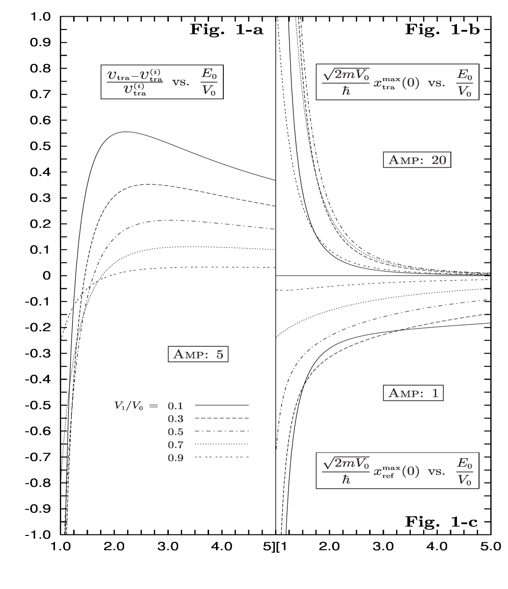
Figure 1: Fixed the value of $V_{\mbox{\tiny$0$}}=|iV_{\mbox{\tiny$1$}}+jV_{\mbox{\tiny$2$}}+kV_{\mbox{\tiny$3$}}|$ and varying its complex component $V_{\mbox{\tiny$1$}}$, the group velocity of the transmitted wave packet, Fig.1-a, and the transmission/reflection times, Fig.1-b and Fig.1-c, are plotted as a function of $E_{\mbox{\tiny$0$}}/V_{\mbox{\tiny$0$}}$, where $E_{\mbox{\tiny$0$}}$ is the maximum of the energy spectrum of the incident wave packet. The analysis is done for diffusion phenomena ($E_{\mbox{\tiny$0$}}>V_{\mbox{\tiny$0$}}$).

References

• [1] S. L. Adler, Quaternionic quantum mechanics and quantum fields, (New York: Oxford University Press, 1995).
• [2] A. J. Davies and B. H. McKellar, “Non-relativistic quaternionic quantum mechanics”, Phys. Rev. A 40, 4209–4214 (1989).
• [3] A. J. Davies and B. H. McKellar, “Observability of quaternionic quantum mechanics”, Phys. Rev. A 46, 3671–3675 (1992).
• [4] S. De Leo, G. Ducati and C. Nishi, “Quaternionic potential in non-relativistic quantum mechanics”, J. Phys. A 35, 5411–5426 (2002).
• [5] S. De Leo and G. C. Ducati, “Quaternionic bound states”, J. Phys. A 38, 3443–3454 (2005).
• [6] S. De Leo, G. C. Ducati, and T. M. Madureira “Analytic plane wave solutions for the quaternionic potential step”, to appear in J. Math. Phys. (August, 2006).
• [7] A. Peres, “Proposed test for complex versus quaternion quantum theory”, Phys. Rev. Lett. 42, 683–686 (1979).
• [8] H. Kaiser, E. A. George and S. A. Werner, “Neutron interferometric search for quaternions in quantum mechanics”, Phys. Rev. A 29, 2276–2279 (1984).
• [9] A. G. Klein, “Schrödinger inviolate: neutron optical searches for violations of quantum mechanics”, Physica B 151, 44–49 (1988).
• [10] S. De Leo and G. Scolarici, “Right eigenvalue equation in quaternionic quantum mechanics”, J. Phys. A 33, 2971–2995 (2000).
• [11] S. De Leo, G. Scolarici and L. Solombrino, “Quaternionic eigenvalue problem”, J. Math. Phys. 43, 5812–2995 (2002).
• [12] S, De Leo and G. C. Ducati , “Quaternionic differential operators”, J. Math. Phys. 42, 2236–2265 (2001).
• [13] S, De Leo and G. C. Ducati , “Solving simple quaternionic differential equations”, J. Math. Phys. 44, 2224-2233 (2003).
• [14] S, De Leo and G. C. Ducati , “Real linear quaternionic differential operators”, Comp. Math. Appl. 48, 1893-1903 (2004).
• [15] A.W. Conway, ”Quaternion treatment of the electron wave equation”, Proc. Roy. Soc. A 162, 145 154 (1937).
• [16] A.W. Conway, ”Quaternions and quantum mechanics”, Acta Pont. Acad. Scien. 12 259 277 (1948).
• [17] S. De Leo, ”One component Dirac equation”, Int. J. Mod. Phys. A 11, 3973-3985 (1996).
• [18] S. De Leo and W. A. Rodrigues, ”Quantum mechanics: from complex to complexified quaternions”, Int. J. Theor. Phys. 36, 2725-2757 (1997).
• [19] S. De Leo and W. A. Rodrigues, ”Quaternionic electron theory: Dirac’s equation”, Int. J. Theor. Phys. 37, 1511-1529 (1998).
• [20] S. De Leo and W. A. Rodrigues, ”Quaternionic electron theory: geometry, algebra and Dirac’s spinors”, Int. J. Theor. Phys. 37, 1707-1720 (1998).
• [21] S. De Leo, W. A. Rodrigues and J. Vaz, ”Complex geometry and Dirac equation”, Int. J. Theor. Phys. 37, 2415-2431 (1998).
• [22] D. Hestenes, Spacetime algebra (New York: Gordon and Breach, 1966).
• [23] A. Lasenby, C. Doran, and S. Gull, ”A multivector derivative approach to Lagrangian field theory”, Found. Phys. 23, 1295 1327 (1993).
• [24] S. Gull, C. Doran, and A. Lasenby, ”Electron paths, tunneling and diffraction in the spacetime algebra”, Found. Phys. 23, 1329 1356 (1993).
• [25] S. De Leo, Z. Oziewicz, W.A. Rodrigues, and J. Vaz, ”Dirac Hestenes Lagrangian”, Int. J. Th. Phys. 38, 2349 2369 (1999).
• [26] A. Lasenby and J. Lasenby, ”Applications of geometric algebra in physics and links with engineering”, 430 457, in E.B. Corrochano and G. Sobczyk, Geometric Algebra with Applications in Science and Engineering (Boston: Birkhauser, 2001) .
• [27] S. De Leo and K. Abdel-Khalek, ”Octonionic quantum mechanics and complex geometry”, Prog. Theor. Phys. 96, 823-831 (1996); ”Octonionic Dirac equation”, ibidem 833-845 (1996).
• [28] S. De Leo and K. Abdel-Khalek, ”Octonionic representations of GL(8,R) and GL(4,C)”, J. Math. Phys. 38, 582-598 (1997).
• [29] J. Soucek, Quaternion quantummechanics as a true 3+1dimensional theory of tachyons, J. Phys. A 14 (1981) 1629 1640.
• [30] J. Soucek, Quaternion quantum mechanics as a description of tachyons and quarks, Czech. J. Phys. B 29 (1979) 315 318.
• [31] S.L. Adler, ”Quaternionic quantum field theory”, Phys. Rev. Lett. 55, 783 786 (1985).
• [32] S.L. Adler, ”Quaternionic quantum field theory”, Comm. Math. Phys. 104, 611 656 (1986).
• [33] P. T. Matthews, Introduction to quantum mechanics, (New York: McGraw-Hill, 1963).
• [34] E. Merzbacher, Quantum mechanics, (New York: John Wiley $\&$ Sons, 1970).
• [35] C. Choen-Tannoudji, B. Diu and F. Lalöe, Quantum mechanics, (New York: John Wiley $\&$ Sons, 1977).
• [36] T.E. Hartman, “Tunnelling of a wave packet”, J. Appl. Phys. 33, 3427-3432 (1962).
• [37] A. Anderson, “Multiple scattering approach to one-dimensional potential problem”, Am. J. Phys. 57, 230-235 (1989).
• [38] A. Pablo, L. Barbero, H.E. Hernández-Figueroa, and E. Recami, ”Propagation speed of evanescent modes”, Phys. E 62, 8628-8635 (2000).
• [39] A. Bernardini, S. De Leo and P. Rotelli, “Above barrier potential diffusion”, Mod. Phys. Lett. A 19, 2717-2725 (2004).
• [40] V.S. Olkhovsky, E. Recami, and J, Jakiel, “Unified time analysis of photon and particle tunnelling”, Phys. Rep. 398, 133-178 (2004).
• [41] S. De Leo and P. Rotelli, “Above barrier Dirac multiple scattering and resonances”, Eur. Phys. J. C 46, 551-558 (2006).
• [42] S. De Leo and P. Rotelli, “Barrier paradox in the Klein zone”, Phys. Rev. A 73, 042107-7 (2006).
Refer to caption