Rigorous conditions for the existence of bound states at the threshold in the two-particle case.

Abstract

In the framework of non-relativistic quantum mechanics and with the help of the Greens functions formalism we study the behavior of weakly bound states as they approach the continuum threshold. Through estimating the Green’s function for positive potentials we derive rigorously the upper bound on the wave function, which helps to control its falloff. In particular, we prove that for potentials whose repulsive part decays slower than $1/r^{2}$ the bound states approaching the threshold do not spread and eventually become bound states at the threshold. This means that such systems never reach supersizes, which would extend far beyond the effective range of attraction. The method presented here is applicable in the many–body case.

I Introduction

In many problems of quantum mechanics it is important to know what happens to the wave function of a system as the bound state approaches the dissociation (decay) threshold. In particular, how does the size of the system in the ground state change as the system becomes loosely bound. Among multiple examples of loosely bound systems in physics one could mention negative atomic and molecular ions hogreve , Efimov states efimov and halo nuclei zhukov , fedorov .

For a bound state of the system as it approaches the threshold there could be two possibilities. The first one is that the probability distribution given by this bound state spreads, meaning that the probability to find all particles together in the fixed bounded region of space goes to zero (the size of the system goes to infinity). One observes such spreading in helium dimer dimer or in halo nuclei like ⁶He or ¹¹Li, which are so loosely bound that two neutrons are about to leave the system and form dilute nuclear matter around the core nucleus (⁴He and ⁹Li respectively) zhukov . The second possibility is that the bound state does not spread and in this case it eventually becomes a bound state at the threshold (the size of the system remains finite). This phenomenon is called the eigenvalue absorption. This is the case for doubly negative ions and proton halos hogreve , fedorov .

Recall, that for two particles interacting through spherically symmetric potentials with finite range $\it S$–states always spread, while all states with non-zero angular momentum become bound klaus . Incidentally, it is natural to conjecture that the ground state of a multi-particle system with pair interactions of finite range ($V_{ij}(x)=0$ for $|x|\geq R$) cannot be bound at the threshold given that the particles are either bosons or distinguishable. For fermions with short-range interactions it is hard to say from general principles whether the ground state would spread or not. The physical approach in this case is to use some kind of shell model and to figure out if there is a centrifugal barrier, which prevents the wave function from spreading.

On the other hand, there are potentials, for which bound states do not spread at all and when approaching the continuum they give rise to bound states exactly at the threshold amer , gest . In particular, the physically important case of repulsive Coulomb tail case belongs to this type (see the discussion in newton ). Let us illustrate this situation by a simple example. Consider the square well potential plus a repulsive Coulomb tail, as in Fig. 1 (left), and imagine the ground state in this potential as it approaches the threshold. The probability distribution for this state would remain a confined wave packet regardless of how small is the binding energy. For zero binding energy there would be a bound state, which would have a falloff of the type $\sim\exp(-\sqrt{r})$. On the contrary, if we cut off the positive tail at some arbitrary distance $R_{c}$, the ground state approaching the threshold would eventually spread when the binding energy is sufficiently small, i.e. the probability to find the particle in some bounded region of space goes to zero with the binding energy. The state “tunnels” through the barrier. Note that this change in the behavior does not depend on the value of $R_{c}$, which could be as large as pleased, so this effect is solely due to the repulsive Coulomb tail. This requires a special care in numerical calculations of loosely bound systems, because often in the calculations the potential becomes effectively cut off.

A rigorous proof of the eigenvalue absorption in the case of a general short-range potential plus a repulsive Coulomb tail was given in gest . Unfortunately, the approach presented in gest , based on the Green’s function expansion, is aimed specifically at the Coulomb long-range part and does not allow generalizations, for example, to potentials having long-range parts of the form $r^{-1}+Ar^{-2}$, which may arise in multipole expansions. Here, we shall consider a more general two-body case. The analysis in amer illuminates the possibilities for various radially dependent long-range parts. However, the arguments given there are not rigorous. Finally, we should mention, that the phenomenon of the ground state absorption was proved rigorously in ostenhof for a three-body system with pure Coulomb interactions and the infinitely massive core. This makes one conjecture that at the point of critical charge negative ions have bound states at the threshold, see the discussion in hogreve . In a forthcoming article we shall give the rigorous proof of this conjecture for distinguishable particles and bosons later , see also the discussion concerning many-body systems in the last section.

The paper is organized as follows. In Sec. II we set the criterium for the eigenvalue absorption. In Sec. III we derive useful upper bounds for the Green’s function. These bounds can also be used to control numerical solutions. In Sec. IV we prove our main result saying that potentials decaying slower as $1/r^{2}$ give rise to bound states at the threshold. The last section presents conclusions and a short discussion concerning many-body systems. Finally, the Appendix contains technical details necessary for the proof in Sec. II.

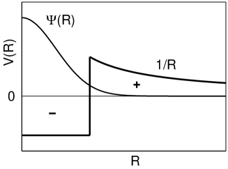
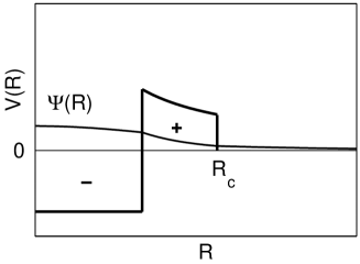
Figure 1: Sketched behavior of the ground state wave functions approaching the threshold in two potentials. Left: the potential has a positive Coulomb tail. Right: the same potential is cut off at some distance $R_{c}$.

II Bound States near Threshold

In nature we can make the bound state of the system approach the threshold by changing the number and the type of particles. In theory we reproduce this behavior changing continuously some parameters in the system. For example, in the case of ions diminishing the atomic charge $Z$ down to the critical value $Z=Z_{cr}$ makes the ground state approach the threshold hogreve . Here, for parameter, changing which we force the states approach the threshold, we take the coupling constant of the interaction.

In our analysis we shall consider the Hamiltonian of two particles $H=H_{0}+\lambda W$, where $H_{0}=p^{2}$ is the free Hamiltonian (we use the units where $\hbar=1$ and $m=1/2$), $W$ is the interaction and $\lambda$ is a coupling constant. By decreasing $\lambda$ we can lift any bound state to the continuum. For convenience we shall consider only $W\in L^{2}(\mathbb{R}^{3})+L^{\infty}(\mathbb{R}^{3})$ reed . This is a large class of interactions, which allows singularities not worse than $r^{-\alpha}$ for $\alpha<3/2$. In this case $H$ is self-adjoint on the domain $D(H_{0})=D(-\Delta)$ reed . However, one could extend our results to potentials having singularities of the type $r^{-\alpha}$ for $\alpha<2$.

Let us assume that there is a bound state having the energy $E(\lambda)<0$ for some value of the coupling constant $\lambda$ . $E(\lambda)$ increases monotonously when $\lambda$ decreases and eventually $E(\lambda)$ becomes zero for $\lambda=\lambda_{cr}$, where $\lambda_{cr}$ is called the critical coupling constant klaus . In the following we show, using a simple example, how the wave function spreads in the case of exponentially decaying potentials. In this simple case the analyticity of the energy as a function of $\lambda$ helps us to establish an upper bound on the wave function

Theorem 1.

If there exist $A,a>0$ such that $|W|\leq Ae^{-a|x|}$ and at $\lambda=\lambda_{cr}$ there is no zero-energy bound state then the following upper bound holds for the bound state $\psi$ having the energy $E(\lambda)$ in the neighborhood of $E(\lambda_{cr})=0$

$$|\psi|\leq\frac{C|E|^{1/4}e^{-\sqrt{|E|}r}}{r},$$ (1)

where $C>0$ is some constant.

Proof.

$\psi$ satisfies the integral equation $\psi=-[H-E]^{-1}W\psi$, which could be rewritten as

$$\psi(x)=-\lambda\int dy\>\frac{e^{-\sqrt{|E|}|x-y|}W(y)\psi(y)}{4\pi|x-y|}$$ (2)

Using $|W|\leq Ae^{-a|x|}$ and applying the Schwarz inequality to Eq. (2) gives us

$$|\psi|\leq\lambda\left<\psi||W||\psi\right>^{1/2}\left[\int dy\>\frac{Ae^{-a|y|}e^{-2\sqrt{|E|}|x-y|}}{|x-y|^{2}}\right]^{1/2}\leq\lambda\left<\psi||W||\psi\right>^{1/2}\frac{C^{\prime}e^{-\sqrt{|E|}r}}{r}$$ (3)

where $C^{\prime}$ is some constant and $r=|x|$. On the other hand, recall klaus that at $\lambda=\lambda_{cr}$ the energy $E(\lambda)$ is analytic and can be expanded into convergent power series $E(\lambda)=\sum_{k=2}^{\infty}a_{k}(\lambda-\lambda_{cr})^{k}$, where $a_{2}<0$ ($a_{1}=0$ because by condition there is no zero-energy bound state at $\lambda=\lambda_{cr}$). Applying the Hellman-Feynman theorem $\left<\psi|H_{0}|\psi\right>=E(\lambda)-\lambda dE/d\lambda$ gives us $\left<\psi|H_{0}|\psi\right>/|E|^{1/2}=O(1)$. Because $|W|\leq Ae^{-a|x|}$ there must exist such constant $L$ that $|W|\leq L(2r)^{-2}$ and thus by the uncertainty principle reed , courant $\left<\phi||W||\phi\right>\leq L\left<\phi|H_{0}|\phi\right>$ for any $\phi\in D(H_{0})$. Thus $\left<\psi||W||\psi\right>/|E|^{1/2}=O(1)$, which together with Eq. (3) proves the statement. ∎

As one can easily see, the function on the right-hand side of Eq. (1) dominates the wave function and spreads as $E\to 0$ maintaining the constant norm independent of $E$. The probability to find the particle in some fixed region of space goes to zero.

Now, let us consider potentials with positive tails. Throughout the paper we shall assume for such potentials that $W(x)\geq 0$ for $|x|\geq R_{0}$, i.e., that outside some sphere the positive part dominates. Below we present a simple criterion, which tells us when bound states become bound states at the threshold. From the discussion above and from Theorem 1 it is clear that the strategy could be proving that as $\lambda\searrow\lambda_{cr}$ bound states remain confined in some region of space, i.e. do not spread. One way to achieve this is to show that bound states are dominated by some fixed function $g\in L^{2}$.

Theorem 2.

Let $\lambda_{n}$ be a sequence of coupling constants and $\lambda_{n}\searrow\lambda_{cr}$. The following is true (a) if for each $\lambda_{n}$ there is a bound state $\phi_{n}$ with the energy $E_{n}$ such that $|\phi_{n}|\leq g$, where $g\in L^{2}$ and $E_{n}\to 0$ then there exists a normalized bound state at the threshold, that is $\phi_{0}\in D(H)$ and $H(\lambda_{cr})\phi_{0}=0$. (b) if for each $\lambda_{n}$ there are $m$ orthogonal bound states $\phi^{(m)}_{n}$ with the energies $E^{(m)}_{n}$ such that $|\phi^{(m)}_{n}|\leq g$, where $g\in L^{2}$ and $\lim_{n\to\infty}E^{(m)}_{n}=0$ then there exist $m$ orthonormal bound states at the threshold.

The proof of this theorem, which follows the method in simon , is given in the Appendix. Intuitively, this proposition is obvious. If the states do not spread they should finally form some bound state at the threshold. A similar theorem concerning many-body systems appeared in Zhislin and Zhizhenkova zhislin . There the authors proved that if a minimizing sequence for the energy functionals does not spread, then there exists a minimizer in $L^{2}$. Their result could be explained from practitioners point of view. Imagine that the system has no bound states with negative energy. Then, if the function minimizing the energy functional, does not go to zero as the number of basis functions increases, then there must exist a zero-energy bound state.

Now let us see how the criterion in Theorem 2 works. First, we separate positive and negative parts of the potential $W=W_{+}-W_{-}$, where $W_{+}=\max(0,W)$ and $W_{-}=\max(0,-W)$ and $W_{\pm}\geq 0$. The equation for the bound states reads $H(\lambda)\phi=-k^{2}\phi$, where $k\to 0$ as $\lambda\to\lambda_{cr}$. This can be rewritten as

$$(H_{0}+k^{2}+\lambda W_{+})\phi=\lambda W_{-}\phi$$ (4)

or equivalently

$$\phi=\lambda(H_{0}+k^{2}+\lambda W_{+})^{-1}W_{-}\phi$$ (5)

The operator $(H_{0}+k^{2}+\lambda W_{+})^{-1}$ is an integral operator, whose kernel is positive and real mark . Thus we can rewrite Eq. (5) as

$$|\phi|\leq 2\lambda_{cr}(H_{0}+k^{2}+\lambda W_{+})^{-1}W_{-}|\phi|,$$ (6)

where because $\lambda\searrow\lambda_{cr}$ we have taken $\lambda\leq 2\lambda_{cr}$ without loss of generality. If we show that the right-hand side of Eq. (6) is bounded by some fixed square integrable function, then according to Theorem 2 we would have bound states at the threshold. The operator $(H_{0}+k^{2}+\lambda W_{+})^{-1}$ is an integral operator, and its kernel is the Green’s function having two arguments. Because the function $W_{-}|\phi|$ vanishes outside some sphere, the behavior of $|\phi|$ at infinity is determined by the asymptotic of the Green’s function when the integration argument is fixed within the sphere. Thus to find the asymptotic we need to derive upper and lower bounds on the Green’s function.

III Bounds on the Green’s Functions

III.1 Potential tails decaying as $1/r^{2}$

III.1.1 Upper Bound

We introduce the function which would play the role of potential’s tail:

$$\eta(A,R_{0};x)=\left\{\begin{array}[]{ll}0&\quad\textrm{if $r<R_{0}$}\\ Ar^{-2}&\quad\textrm{if $r\geq R_{0}$},\\ \end{array}\right.$$ (7)

We are interested in the kernel of the integral operator $[H_{0}+k^{2}+\eta(A,R_{0};x)]^{-1}$ for $k$ real, which we denote as $G_{k}(A,R_{0};x,y)$. Note that the kernel of such operator is a positive function, continuous away from $x=y$ mark . Our aim in this section is to find the upper bound on $G_{k}(A,R_{0};x,y)$. For that we need the following lemma

Lemma 1.

Let $G_{1,2}(x,y)$ denote the integral kernels of $[H_{0}+k^{2}+V_{1,2}]^{-1}$ and suppose $V_{1}(x)\leq V_{2}(x)$. Then $G_{2}(x,y)\leq G_{1}(x,y)$.

Proof.

Through the integral representation we get

$$G_{2}(x,y)=G_{1}(x,y)-\int dy^{\prime}G_{1}(x,y^{\prime})[V_{2}(y^{\prime})-V_{1}(y^{\prime})]G_{2}(y^{\prime},y)$$ (8)

Eq. (8) is the kernel representation of the equation $(A+B)^{-1}=A^{-1}-A^{-1}B(A+B)^{-1}$, where $A=H_{0}+k^{2}+V_{1}$ and $B=V_{2}-V_{1}$. Now, because $G_{1,2}(x,y)$ are positive mark and the potential difference $V_{2}-V_{1}$ is non-negative, the integral in Eq. (8) must be non-negative and the statement is proved. ∎

There is another elucidating and more direct way to prove Lemma 1. The proposition of the Lemma follows from the Laplace transform and the Trotter product formula, which lie at the heart of path-integrals reed

$$(H_{0}+k^{2}+V_{1})^{-1}=\int^{\infty}_{0}e^{-k^{2}t}e^{-t(H_{0}+V_{1})}dt$$ (9)

$$e^{-t(H_{0}+V_{1})}=\text{s-}\negthinspace\lim_{m\to\infty}\left[e^{-tH_{0}/m}e^{-tV_{1}/m}\right]^{m}$$ (10)

Because $e^{-tH_{0}}$ in Eq. (10) has a positive kernel, namely $(4\pi t)^{-3/2}e^{-|x-y|^{2}/4t}$, the kernel of the operator on the left in Eq. (10) becomes smaller when $V_{1}$ is replaced by $V_{2}$.

The idea behind the upper bound on the Green’s function is rather simple. Suppose we have found such a function $F(A,R_{0},x)$, independent of $k$, so that $G_{k}(A,R_{0};x,0)\leq F(A,R_{0};x)$ holds for all $k$ and $x$. First, we shall derive the upper bound in terms of the function $F$, and then we shall determine $F$ explicitly.

Let us fix the functions $\tilde{A}(s),\tilde{R}_{0}(s)$ so that the following inequality holds

$$\eta(A,R_{0};x)\geq\eta(\tilde{A},\tilde{R}_{0};x-s),$$ (11)

where $s$ is some fixed three–dimensional vector. From simple geometric arguments it follows that Eq. (11) would be satisfied if $\tilde{A}(s),\tilde{R}_{0}(s)$ satisfy the inequalities

$$\tilde{R}_{0}(s)\geq R_{0}+|s|$$ (12)

$$\tilde{A}(s)\leq A\frac{\tilde{R}_{0}^{2}}{(\tilde{R}_{0}+|s|)^{2}}$$ (13)

Let us mention that the closer $\tilde{A}$ is to $A$ the better is the asymptotic behavior of the bound, hence it is reasonable to take $\tilde{R}_{0}$ large.

Translating the arguments one finds that $G_{k}(\tilde{A},\tilde{R}_{0};x-s,y-s)$ is the integral kernel of the operator $[H_{0}+k^{2}+\eta(\tilde{A},\tilde{R}_{0};x-s)]^{-1}$. Now, using Eq. (11) and Lemma 1 we obtain the upper bound

$$G_{k}(A,R_{0};x,y)\leq G_{k}(\tilde{A},\tilde{R}_{0};x-s,y-s)$$ (14)

Eq. (14) is valid for all $s$, so we can put $s=y$, which gives us

$$G_{k}(A,R_{0};x,y)\leq F(\tilde{A}(y),\tilde{R}_{0}(y);x-y)$$ (15)

It remains to find $F$, which is the upper bound on $G_{k}(A,R_{0};x,0)$. This is easy because $G_{k}(A,R_{0};x,0)$ is spherically symmetric in $x$. From now on for simplicity of notation we shall drop $A,R_{0}$ in the arguments, writing, for example, $F(x)$ instead of $F(A,R_{0};x)$. First, we shall give a formal solution, then we shall prove that this solution is indeed correct. By Lemma 1 $G_{k}(x,0)\leq G_{k^{\prime}}(x,0)$ if $k^{\prime}\leq k$, so we can take $F(x)=\lim_{k\to 0}G_{k}(x,0)$. Because $G_{k}(x,0)$ is continuous away from $x=0$ mark and the functions $G_{k}(x,0)$ increase monotonically when $k\to 0$ the pointwise limit makes sense. By Lemma 1 $G_{k}(x,0)\leq G^{(0)}_{k}(x,0)$, where $G^{(0)}_{k}(x,y)=(4\pi|x-y|)^{-1}\exp{(-k|x-y|)}$ is the free propagator, i.e. the integral kernel of the operator $[H_{0}+k^{2}]^{-1}$. This means $F(x)$ is bounded away from $x=0$ and $F(x)\leq(4\pi r)^{-1}$. Because $G_{k}(x,y)$, formally satisfies the equation $[H_{0}+k^{2}+\eta]G_{k}(x,y)=\delta(x-y)$ one expects that $F(x)$ satisfies the equation

$$[H_{0}+\eta]F=\delta(x)$$ (16)

To find the solution of Eq. (16) we set

$$F=\frac{1}{4\pi r}\times\left\{\begin{array}[]{ll}1+br&\quad\textrm{if $r\leq R_{0}$}\\ cr^{-a}&\quad\textrm{if $r\geq R_{0}$},\\ \end{array}\right.$$ (17)

where $a$ is the positive root of the equation $a(a+1)=A$ and the constants $b,c$ are fixed requiring, as usual, that $F$ and its derivative are continuous at $r=R_{0}$. This gives us

$$F(A,R_{0};x)=\frac{1}{4\pi r}\times\left\{\begin{array}[]{ll}1-R^{-1}_{0}a(a+1)^{-1}r&\quad\textrm{if $r\leq R_{0}$}\\ R_{0}^{a}(1+a)^{-1}r^{-a}&\quad\textrm{if $r\geq R_{0}$}\\ \end{array}\right.$$ (18)

One can check that $F(x)$ defined by Eq. (18) indeed satisfies Eq. (16).

For completeness we give the accurate proof, which justifies Eq. (18).

Lemma 2.

$F(x)$ defined as $F(x)=\lim_{k\to 0}G_{k}(x,0)$ equals a.e. the expression given by Eq. (18).

Proof.

The integral equation for the resolvent reads reed

$$G_{k}(x,y)=G^{(0)}_{k}(x,y)-\int dy^{\prime}G^{(0)}_{k}(x,y^{\prime})\eta(y^{\prime})G_{k}(y^{\prime},y)$$ (19)

Substituting the expression for $G^{(0)}_{k}(x,y)$ and setting $y=0$ we obtain

$$G_{k}(x,0)=\frac{e^{-kr}}{4\pi r}-\frac{1}{4\pi}\int dy^{\prime}\frac{e^{-k|x-y^{\prime}|}}{|x-y^{\prime}|}\eta(y^{\prime})G_{k}(y^{\prime},0)$$ (20)

Applying $\lim_{k\to 0}$ to both sides of Eq. (20) gives us the integral equation

$$F(x)=\frac{1}{4\pi r}-\frac{1}{4\pi}\int dy^{\prime}\frac{\eta(y^{\prime})}{|x-y^{\prime}|}F(y^{\prime})$$ (21)

By simple substitution and calculating the integrals one can check that $F$ given by Eq. (18) indeed solves the integral equation Eq. (21). It remains to prove that no other solution exists. Suppose there are two solutions and denote their difference $Z=F_{1}-F_{2}$. Then $Z$ satisfies the integral equation

$$Z(x)=-\frac{1}{4\pi}\int dy^{\prime}\frac{1}{|x-y^{\prime}|}\eta(y^{\prime})Z(y^{\prime})$$ (22)

We need to show that $Z=0$ a.e. Let $\tilde{Z}=\eta^{1/2}Z$, then $\tilde{Z}\in L^{2}$ by the dominated convergence theorem and $\|\tilde{Z}\|\neq 0$, because otherwise from Eq. (22) it follows $Z=0$ and we are done. From Eq. (22) we obtain

$$\int dxdy\frac{\eta^{1/2}(x)\tilde{Z}(x)\eta^{1/2}(y)\tilde{Z}(y)}{|x-y|}=-\|\tilde{Z}\|^{2}<0$$ (23)

But Eq. (23) cannot hold because $|x-y|^{-1}$ is the kernel of the strictly positive operator. This means Eq. (22) holds only if $Z=0$.∎

Now let us formulate the bound in the form required in Sec. IV.

Corollary 1.

Let $A>3/4$, then there exist $C>0$, $\delta>0$ and $R$ such that for $|y|\leq R_{0}$ and $|x|\geq R$ the inequality holds $G_{k}(A,R_{0};x,y)\leq C|x|^{-3/2-\delta}$.

Proof.

For $|y|\leq R_{0}$ we can fix the values $\tilde{R}_{0}$ and $\tilde{A}$ independent of $y$. Both inequalities Eq. (12), (13) would be satisfied if $\tilde{R}_{0}\geq 2R_{0}$ and $\tilde{A}\leq A\tilde{R}_{0}^{2}(\tilde{R}_{0}+R_{0})^{-2}$. When $\tilde{R}_{0}$ becomes large $\tilde{A}$ gets close to $A$, so we can fix the values of $\tilde{R}_{0}$ and $\tilde{A}$ to ensure that the following inequality holds $3/4<\tilde{A}<A$. If we set $R=\tilde{R}_{0}+R_{0}$, then for $|y|\leq R_{0}$ and $|x|\geq R$ we have $|x-y|\geq\tilde{R}_{0}$ and from Eq. (15), (18) we get

$$G_{k}(A,R_{0};x,y)\leq(4\pi|x|)^{-1}\tilde{R}^{\tilde{a}}_{0}(1+\tilde{a})^{-1}|x-y|^{-\tilde{a}}\leq C|x|^{-1-\tilde{a}},$$ (24)

where $\tilde{a}$ is the positive root of the equation $\tilde{a}(\tilde{a}+1)=\tilde{A}$, $\tilde{a}>1/2$.∎

III.1.2 Lower Bound

Here we shall briefly discuss how the same method can be applied to construction of lower bounds. We would need this in Section IV where we show that the ground state of potentials decaying faster than $(3/4)r^{-2}$ spreads near the point of critical binding. For that we need the following type of potential

$$\xi(A,R_{0},;x)=\left\{\begin{array}[]{ll}V_{0}&\quad\textrm{if $r<R_{0}$}\\ Ar^{-2}&\quad\textrm{if $r\geq R_{0}$},\\ \end{array}\right.$$ (25)

and we need the upper bound for Green’s function of the operator $\Xi_{k}(A,R_{0})=[H_{0}+\xi+k^{2}]^{-1}$, which has the integral kernel $\Xi_{k}(A,R_{0};x,y)$. We shall derive the lower bound in terms of the function $f_{k}(A,R_{0};r)=\Xi_{k}(A,R_{0};x,0)$, which falls off at infinity and solves the following equation

$$\left[H_{0}+\xi+k^{2}\right]f_{k}=\delta(x)$$ (26)

$f_{k}$ depends only on $r=|x|$ (because the potential is spherically symmetric) and is a continuous function away from $r=0$. By definition of $f_{k}$ we have $0<f_{k}\leq 1/(4\pi r)$. Setting $f_{k}=(4\pi r)^{-1}\hat{f}_{k}$ from Eq. (26) we obtain the equation on $\hat{f}_{k}$

$$-\hat{f}_{k}^{\prime\prime}+\xi\hat{f}_{k}+k^{2}\hat{f}_{k}=0$$ (27)

with the boundary conditions $\hat{f}_{k}(0)=1$ and $\hat{f}_{k}(\infty)=0$. The function $0<\hat{f}_{k}(r)\leq 1$ comes out as a solution of a simple radial equation and thus can be easily calculated. As usual, one calculates the solutions $\hat{f}_{k}(r<R_{0})$ and $\hat{f}_{k}(r>R_{0})$ and determines the constants so that $\hat{f}_{k}$ and its derivative are continuous at $R_{0}$. The following Lemma is useful for the lower bound.

Lemma 3.

For $r\geq R_{0}$ there exists $C_{0}$ independent of $k$ such that

$$\hat{f}_{k}(r)\geq C_{0}e^{-kr}r^{-a}$$ (28)

Proof.

According to Eq. (27) on the interval $[R_{0},\infty]$ the function $\hat{f}_{k}$ satisfies the equation

$$-\hat{f}_{k}^{\prime\prime}+Ar^{-2}\hat{f}_{k}+k^{2}\hat{f}_{k}=0$$ (29)

Let us set $\hat{f}_{k}(r)=g_{k}(r)e^{-kr}r^{-a}$. Then for $g_{k}(r)$ on the interval $[R_{0},\infty]$ the equation becomes

$$-g_{k}^{\prime\prime}+2\left(ar^{-1}+k\right)g_{k}^{\prime}=2akr^{-1}g_{k}$$ (30)

Because $f_{k}$ is positive $g_{k}$ should be also positive. Hence from Eq. (30) we get

$$g_{k}^{\prime\prime}\leq 2\left(ar^{-1}+k\right)g_{k}^{\prime}$$ (31)

We want to show that $g_{k}^{\prime}\geq 0$. Indeed, if on the contrary $g_{k}^{\prime}(y)<0$ at some point $y$, then at this point due to Eq. (31) $g_{k}^{\prime\prime}(y)<0$. Hence $g^{\prime}$ is a monotonically decreasing function for $r\geq y$. Thus from Eq. (31) we conclude that $g_{k}^{\prime\prime}\leq 2kg_{k}^{\prime}(y)$ for all $r>y$, i.e. the second derivative is less than a fixed negative value, which means that at some point $g_{k}$ becomes negative. Hence the assumption was false and $g_{k}^{\prime}\geq 0$ holds. On the other hand, $f_{k}>0$ and as $k\to 0$ the function $f_{k}$ monotonically increases in all points. Hence, there must exist $C_{0}>0$ such that $g_{k}(R_{0})\geq C_{0}$. Together with $g_{k}^{\prime}\geq 0$ this means that $g_{k}$ stays above $C_{0}$ and Eq. (28) holds. ∎

Now we follow the above procedure and define $\tilde{A},\tilde{R}_{0}$ as satisfying the inequality

$$\xi(\tilde{A},\tilde{R}_{0},;x-s)\geq\xi(A,R_{0},;x)$$ (32)

By geometrical arguments $\tilde{A},\tilde{R}_{0}$ must satisfy

$$\tilde{R}_{0}(s)\geq R_{0}+|s|$$ (33)

$$\tilde{A}(s)\geq A\frac{\tilde{R}_{0}^{2}}{(\tilde{R}_{0}+|s|)^{2}}$$ (34)

Just as in the previous subsection through Eq. (32) we obtain the desired lower bound

$$\Xi_{k}(A,R_{0};x,y)\geq\Xi_{k}(\tilde{A},\tilde{R}_{0};x-y,0)=f_{k}(\tilde{A},\tilde{R}_{0};|x-y|)$$ (35)

Now suppose $A<3/4$. Looking at Eq. (33)–(34) one can see that we can fix $\tilde{R}_{0}$ and $\tilde{A}$ so that $\tilde{A}<3/4$ and Eq. (33)–(34) are valid. Then from Eq. (35) and Lemma 3 it is clear that there exists a constant $C>0$ such that for $|x|\geq 2\tilde{R}_{0}$ and for $|y|\leq R_{0}$ the following inequality holds

$$\Xi_{k}(A,R_{0};x,y)\geq f_{k}(\tilde{A},\tilde{R}_{0};|x-y|)\geq Ce^{-k|x|}|x|^{-3/2}$$ (36)

We would need inequality Eq. (36) in Sec. IV.

III.2 Potential tails decaying as $1/r$

Here we would like to apply the results of the previous section to potentials with positive Coulomb tails. This helps to establish the decay properties of eigenfunctions lying at the threshold. We shall not present a detailed exposition, because everything is similar to the previous section. One can follow in the steps of the previous section and derive the bound in terms of the solution of the equation $[H_{0}+\eta^{\prime}]F=\delta(r)$, where $\eta^{\prime}$ is the Coulomb tail. This however could not be expressed through elementary functions, so we shall make a couple of simplifying approximations. We shall consider the following potential tail.

$$\zeta(a,R_{0};x)=\left\{\begin{array}[]{ll}0&\quad\textrm{if $r<R_{0}$}\\ (a^{2}/4)r^{-1}+(a/4)r^{-3/2}&\quad\textrm{if $r\geq R_{0}$},\\ \end{array}\right.$$ (37)

The repulsive Coulomb tail dominates in the potential of Eq. (37) and one can choose the constants so that the actual Coulomb tail is greater than the function in Eq. (37). Let $G^{c}_{k}(a,R_{0};x,y)$ be the integral kernel of the operator $[H_{0}+k^{2}+\zeta(a,R_{0};x)]^{-1}$, where $c$ stands for Coulomb. The rest follows as above.

Let us fix the functions $\tilde{a}(s),\tilde{R}_{0}(s)$ so that the following inequality holds

$$\zeta(a,R_{0};x)\geq\zeta(\tilde{a},\tilde{R}_{0};x-s),$$ (38)

Again from geometric arguments it follows that Eq. (38) would be satisfied if $\tilde{a}(s),\tilde{R}_{0}(s)$ satisfy the inequalities

$$\tilde{R}_{0}(s)\geq R_{0}+|s|$$ (39)

$$\tilde{a}(s)\leq a\left(\frac{\tilde{R}_{0}}{\tilde{R}_{0}+|s|}\right)^{3/2}$$ (40)

where the above conditions are obtained by directly applying Eq. (38) to each positive term in the expression for $\zeta(a,R_{0};x)$ given by Eq. (37).

Again let us define $F^{c}(x)=\lim_{k\to 0}G^{c}_{k}(x,0)$, which makes $F^{c}(x)$ satisfy the equation

$$[H_{0}+\zeta]F^{c}=\delta(x)$$ (41)

As one can easily check, the solution of Eq. (41) is given by

$$F^{c}(A,R_{0};r)=\frac{1}{4\pi r}\times\left\{\begin{array}[]{ll}1-\frac{1}{R_{0}+2\sqrt{R_{0}}/a}r&\quad\textrm{if $r\leq R_{0}$}\\ \frac{e^{a\sqrt{R_{0}}}}{1+(a/2)\sqrt{R_{0}}}e^{-a\sqrt{r}}&\quad\textrm{if $r\geq R_{0}$}\\ \end{array}\right.$$ (42)

Finally, the upper bound reads

$$G^{c}_{k}(a,R_{0};x,y)\leq F^{c}(\tilde{a}(y),\tilde{R}_{0}(y);x-y),$$ (43)

where $\tilde{a}$ and $\tilde{R}_{0}$ satisfy Eq. (39)-(40). As in Corollary 1 from Eq. (43) we find that there exists such $R>0$ and $C>0$ that

$$G^{c}_{k}(a,R_{0};x,y)\leq Ce^{-a\sqrt{|x|}}\quad\textrm{if $|y|\leq R_{0}$ and $|x|\geq R$}$$ (44)

As we have mentioned for potentials with positive tails the asymptotic of the Green’s function determines the fall-off behavior of bound state wave functions. Hence the bound state wave functions fall off at least as fast as $e^{-a\sqrt{r}}$. Calculating in the same way the lower bound one finds that this is the actual fall-off.

IV Main Result

Now we state the main result of this paper.

Theorem 3.

If there are such $R_{0}$ and $A>3/4$ that $\lambda W_{+}\geq\eta(A,R_{0};x)$ then at $\lambda=\lambda_{cr}$ all states that hit the threshold at $\lambda=\lambda_{cr}$ become zero energy bound states.

Proof.

Let us define $G_{k}(A,R_{0};x,y)$ the positive integral kernel of the operator $[H_{0}+k^{2}+\eta]^{-1}$. Then from Eq. (6) and by Lemma 1 we get the bound

$$|\phi|(x)\leq 2\lambda_{cr}\int_{|y|\leq R_{0}}dy\>G_{k}(A,R_{0};x,y)W_{-}(y)|\phi|(y),$$ (45)

where we have used $W_{-}(y)=0$ for $|y|\leq R_{0}$. Now we shall use the upper bounds on the Green’s function $G_{k}(A,R_{0};x,y)$ derived in Se. III. For $|x|\geq R$ we can use Corollary 1 to obtain from Eq. (45)

$$|\phi|(x)\leq 2\lambda_{cr}C|x|^{-3/2-\delta}\int_{|y|\leq R_{0}}dy\>W_{-}(y)|\phi|(y)\leq C_{1}|x|^{-3/2-\delta}\equiv g_{>}(x),$$ (46)

where we have applied the Schwarz inequality and used $W\in L^{2}+L^{\infty}$. For $|x|\leq R$ we can use $G_{k}(A,R_{0};x,y)\leq(4\pi)^{-1}|x-y|^{-1}$ to obtain from Eq. (45)

$$|\phi|(x)\leq 2\lambda_{cr}(4\pi)^{-1}\int_{|y|\leq R_{0}}dy\>|x-y|^{-1}W_{-}(y)|\phi|(y)$$

$$\leq C_{2}\left[\int_{|y|\leq R_{0}}dy\>|x-y|^{-2}W^{2}_{-}(y)\right]^{1/2}\equiv g_{<}(x),$$ (47)

Thus we get $|\phi|(x)\leq g(x)$, where $g(x)=g_{<}(x)$ for $|x|\leq R$ and $g(x)=g_{>}(x)$ for $|x|>R$. Because $g(x)\in L^{2}$ Theorem 2 applies and the theorem is proved. ∎

One can construct simple examples, which show that the condition in Theorem 3 is best possible. The following theorem is also true.

Theorem 4.

If there exists $R_{0}$ such that

$$W(x)\leq(3/4)|x|^{-2}\;\;\;{\rm for}\;\;|x|\geq R_{0}$$ (48)

then the ground state cannot be bound at the threshold.

Proof.

For simplicity we shall assume that there exists a constant $V_{0}$ such that $W_{+}\leq V_{0}$. A proof by contradiction. Suppose that the ground state $\psi_{0}$ exists. Then the equation for the bound state at the threshold can be written as $[H_{0}+W_{+}]\psi_{0}=W_{-}\psi_{0}$. This is equivalent to the equation $[H_{0}+W_{+}+k^{2}]\psi_{0}=W_{-}\psi+k^{2}\psi_{0}$, which in turn can be transformed into the integral equation

$$\psi_{0}=[H_{0}+W_{+}+k^{2}]^{-1}W_{-}\psi_{0}+k^{2}[H_{0}+W_{+}+k^{2}]^{-1}\psi_{0}$$ (49)

The ground state wave function is always nonnegative $\psi_{0}\geq 0$ reed . Because $W_{-}\geq 0$, $\psi_{0}\geq 0$ in Eq. (49) on the right-hand side we have a sum of two positive terms (the operator $[H_{0}+W_{+}+k^{2}]^{-1}$ has a positive integral kernel). Hence we must have

$$\|[H_{0}+W_{+}+k^{2}]^{-1}W_{-}\psi_{0}\|\leq 1$$ (50)

for all $k$. Because the positive part of $W$ is bounded we have $W_{+}\leq\xi(A,R_{0};x)$, where $\xi$ is defined by Eq. (25).

From Eq. (50) and using Lemma 1 we conclude $\|\Xi_{k}(A,R_{0})W_{-}\psi_{0}\|\leq 1$ for all $k$, where $\Xi_{k}(A,R_{0})=[H_{0}+\xi+k^{2}]^{-1}$. Our aim is to prove $\lim_{k\to 0}\|\Xi_{k}(A,R_{0})W_{-}\psi_{0}\|=\infty$ thus obtaining the desired contradiction. We shall use the lower bound on $\Xi_{k}(A,R_{0};x,y)$ from Sec. III.1.2. Let us fix $\tilde{R}_{0}$ as in the last part of Sec. III.1.2. Then using the bound Eq. (36) we obtain for the square of the norm

$$\|\Xi_{k}W_{-}\psi_{0}\|^{2}\geq\int_{|y_{1}|\leq R_{0}}\int_{|y_{2}|\leq R_{0}}dy_{1}dy_{2}\>W_{-}(y_{1})\psi_{0}(y_{1})W_{-}(y_{2})\psi_{0}(y_{2})$$ (51)

$$\times\int_{|x|\geq 2\tilde{R}_{0}}dx\Xi_{k}(A,R_{0};x,y_{1})\>\Xi_{k}(A,R_{0};x,y_{2})$$ (52)

$$\geq M^{2}C^{2}\int_{|x|\geq 2\tilde{R}_{0}}dx|x|^{-3}e^{-2k|x|}$$ (53)

where $M=\int_{|y|\leq R_{0}}dyW_{-}(y)\psi_{0}(y)$ is some fixed constant. Note that $M\neq 0$ because that would mean $\psi_{0}=0$. It is clear that the right-hand side in Eq. (53) becomes infinitely large as $k\to 0$ and thus $\|\Xi_{k}(A,R_{0})W_{-}\psi_{0}\|\leq 1$ cannot hold for small $k$. ∎

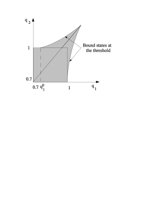
Figure 2: Typical stability diagram (sketch) for three Coulomb charges $\{-1,q_{1},q_{2}\}$, the shaded area representing stable systems. On the arcs of stability curve where either $q_{1}>1$ or $q_{2}>1$ there are bound states at the threshold.

V Conclusions

We have proposed the method to derive lower and upper bounds on the Green’s functions, which helps to determine the fall-off of bound states. Using these bounds we have proved that potentials, whose tails decay as $(2\mu/\hbar^{2})V>(3/4)r^{-2}$, where $\mu$ is the reduced mass, absorb the eigenvalues, meaning that their bound states do not spread and become bound states at the threshold. We have also found that ground states in potentials, whose tails decay as $(2\mu/\hbar^{2})V<(3/4)r^{-2}$, always spread as they approach the continuum.

These methods can be applied to the many-particle case, where it is still not known, for which pair interactions between decaying particles or clusters the bound state would become absorbed. The difficulty is that it is hard to control the asymptotic of the many-body bound state wave function. Using bounds on the Green’s functions derived here one can demonstrate later that when there is a long-range Coulomb repulsion between decaying components (particles or clusters), then the bound state must get absorbed.

Two types of behavior, namely spreading and eigenvalue absorption can be perfectly illustrated by a stability diagram for three Coulomb charges, see martin . When masses are fixed the diagram has the form as in Fig. 2. If we consider, for example, the upper arc, which is the stability border, it has the following property martin . Up to some non-zero value of $q^{0}_{1}$ the stability border is given by the equation $q_{2}=1$. Then at the point $\{q^{0}_{1},1\}$ the arc goes up. With the same method as here it can be proved later that if one approaches the stability border from the side where $q_{2}=1$ then the ground state spreads and there is no bound state at the threshold. On the contrary, for the points on the arc the ground state becomes absorbed, i.e. it does not spread and becomes a bound state at the threshold. The reason is that on the stability border, where $q_{2}=1$ the system decays into a neutral cluster and one charged particle, and for $q_{2}>1$ both cluster and the particle are charged positively. The resulting Coulomb repulsion between these objects hinders the spreading of the wave function and the ground state becomes absorbed. Note that it has already been proved rigorously ostenhof , that in the case of an infinite core and two other masses being equal, the sharp point on the diagram, see Fig. 2, has a bound state at the threshold. Our method helps to extend this result to many particles.

Appendix A Proof of Theorem 2

Proof.

Let us prove part (a). We follow the argument from simon . Because $\|\phi_{n}\|=1$ we can extract a weakly converging subsequence (for which we reserve the same index $n$) such that $\phi_{n}\stackrel{{\scriptstyle w}}{{\to}}\phi_{0}$, where $\phi_{0}\in L^{2}$. Because H is self-adjoint in order to prove that $\phi_{0}\in D(H)$ and $H(\lambda_{cr})\phi_{0}=0$ it is enough to show that for every $f\in D(H)$ we have $\left<H(\lambda_{cr})f|\phi_{0}\right>=0$. The latter we obtain as follows

$$\left<H(\lambda_{cr})f|\phi_{0}\right>=\lim_{n\rightarrow\infty}\left<H(\lambda_{cr})f|\phi_{n}\right>=\lim_{n\rightarrow\infty}[\left<H(\lambda_{n})f|\phi_{n}\right>-(\lambda_{n}-\lambda_{cr})\left<Wf|\phi_{n}\right>]=$$ (54)

$$\lim_{n\rightarrow\infty}\left<f|H(\lambda_{n})\phi_{n}\right>=\lim_{n\rightarrow\infty}E_{n}\left<f|\phi_{n}\right>=0.$$ (55)

The only thing that remains to show is that $\phi_{0}\neq 0$. We shall prove this by contradiction assuming that $\phi_{n}\stackrel{{\scriptstyle w}}{{\to}}0$. Let us introduce $\chi_{R}$, the characteristic function of the interval $[0,R]$ (i.e. $\chi_{R}(x)=1$ when $|x|\in[0,R]$ and $\chi_{R}(x)=0$ otherwise). Because $|\phi_{n}|\leq g$ and $g\in L^{2}$ we can fix $R$ so that $\left<\phi_{n}|\chi_{R}|\phi_{n}\right>>1/2$. We would like to show that for $\phi_{n}\stackrel{{\scriptstyle w}}{{\to}}0$ the condition $\left<\phi_{n}|\chi_{R}|\phi_{n}\right>>1/2$ cannot hold for large $n$. One way to do this is to use that $\int|\nabla\phi_{n}|^{2}dx\leq const$ and apply the Rellich-Kondrashov lemma loss giving $\chi_{R}\phi_{n}\to 0$ strongly. Or we can use the argument similar to the one in simon . Using the equation $(H_{0}+1)\phi_{n}=(E_{n}+1)\phi_{n}-\lambda_{n}W\phi_{n}$ we get $\phi_{n}=(E_{n}+1)(H_{0}+1)^{-1}\phi_{n}-\lambda_{n}(H_{0}+1)^{-1}W\phi_{n}$. Substituting this into $\left<\phi_{n}|\chi_{R}|\phi_{n}\right>>1/2$ we obtain

$$(E_{n}+1)\left<\phi_{n}|\chi_{R}(H_{0}+1)^{-1}\phi_{n}\right>-\lambda_{n}\left<\phi_{n}|\chi_{R}(H_{0}+1)^{-1}W\phi_{n}\right>>1/2$$ (56)

The operators $\chi_{R}(H_{0}+1)^{-1}$ and $\chi_{R}(H_{0}+1)^{-1}W$ have square integrable kernels and are therefore compact. Acting on weakly convergent sequences they make them converge strongly and hence both terms on the left-hand side of Eq. (56) go to zero. Thus Eq. (56) cannot hold for large $n$, which proves (a).

Part (b) easily follows if we prove that from $\phi_{n}\stackrel{{\scriptstyle w}}{{\to}}\phi_{0}$ follows $\phi_{n}\to\phi_{0}$ in norm. Indeed, for each $\lambda_{n}$ there are bound states $\phi^{(i)}_{n}$ (i = 1, …, m) satisfying $H(\lambda_{n})\phi^{(i)}_{n}=E^{(i)}_{n}\phi^{(i)}_{n}$. Moreover $\left<\phi^{(i)}_{n}|\phi^{(k)}_{n}\right>=\delta_{ik}$ and as $\lambda_{n}\searrow\lambda_{cr}$ the energies go to zero $E^{(i)}_{n}\to 0$. In this case since $|\phi^{(i)}_{n}|<g\in L^{2}$ there are $m$ bound states at the threshold, $\phi^{(i)}_{n}\stackrel{{\scriptstyle w}}{{\to}}\phi^{(i)}_{0}$. Because this convergence is in norm $\left<\phi^{(i)}_{0}|\phi^{(k)}_{0}\right>=\delta_{ik}$ holds.

To prove that from $\phi_{n}\stackrel{{\scriptstyle w}}{{\to}}\phi_{0}$ follows $\phi_{n}\to\phi_{0}$ in norm let us define $\xi_{n}=\phi_{n}-\phi_{0}$, then $\xi_{n}\stackrel{{\scriptstyle w}}{{\to}}0$ and we would like to show that $\|\xi_{n}\|\to 0$. A proof by contradiction. If not then there must exist a constant $a>0$ and a subsequence (for which we again reserve the same index $n$) such that $\|\xi_{n}\|^{2}>a$. Again because $|\phi_{n}|\leq g$ and $\phi_{0}\in L^{2}$ we can fix $R$ so that $\left<\xi_{n}|\chi_{R}|\xi_{n}\right>>a/2$. We have $\xi_{n}\in D(H)$ and $(H_{0}+\lambda_{n}W)\xi_{n}=E_{n}\phi_{n}+(\lambda_{cr}-\lambda_{n})W\phi_{0}$. From this equation we easily get

$$\xi_{n}=(H_{0}+1)^{-1}\xi_{n}-\lambda_{n}(H_{0}+1)^{-1}W\xi_{n}+E_{n}(H_{0}+1)^{-1}\phi_{n}+(\lambda_{cr}-\lambda_{n})(H_{0}+1)^{-1}W\phi_{0}$$ (57)

Substituting one $\xi_{n}$ from Eq. (57) into $(\xi_{n},\chi_{R}\xi_{n})$ and using that $\chi_{R}(H_{0}+1)^{-1}$ and $\chi_{R}(H_{0}+1)^{-1}W$ are compact and $\xi_{n}\stackrel{{\scriptstyle w}}{{\to}}0$ we obtain $\left<\xi_{n}|\chi_{R}|\xi_{n}\right>\to 0$. This is a contradiction. ∎

- (1) H. Hogreve, J. Phys. B 31, L439 (1998); Phys. Scr. 58, 25 (1998); private communication.
- (2) T. Kraemer, et.al. Nature 440, 315 (2006)
- (3) M.V. Zhukov, B.V. Danilin, D.V. Fedorov, J.M. Bang, I.J. Thompson and J.S. Vaagen, Phys. Rep. 231, 151 (1993).
- (4) F. Lou, C.F. Giese and W.R. Gentry, J. Chem. Phys. 104, 1151 (1996)
- (5) D. V. Fedorov, A. S. Jensen, and K. Riisager, Phys. Rev. C 49, 201 (1994); A. S. Jensen, K. Riisager, and D. V. Fedorov, Rev. Mod. Phys. 76 215 (2004); K. Riisager, D. V. Fedorov and A. S. Jensen, Europhys. Lett. 49, 547 (2000).
- (6) M. Klaus and B. Simon, Ann. Phys. 130, 251 (1980).
- (7) R. K. P. Zia, R. Lipowski and D.M. Kroll, Am. J. Phys. 56, 160 (1998).
- (8) D. Bolle, F. Gesztesy and W.Schweiger, J. Math. Phys 26, 1661 (1985).
- (9) R. Newton, Scattering Theory of Waves and Particles, McGraw-Hill/New York 1966.
- (10) M Hoffmann-Ostenhof, T Hoffmann-Ostenhof and B Simon, J. Phys. A 16, 1125 (1983).
- (11) D. K. Gridnev and M. Garcia, to appear in Phys. Rev. A.
- (12) M. Reed and B. Simon, Methods of Modern Mathematical Physics, vol. 2-4, Academic Press/New York (1978)
- (13) R. Courant and D. Hilbert, Methods of Mathematical Physics, Interscience Publishers, New York, (1953), vol. 1, p. 446
- (14) B. Simon, J. Functional Analysis 25, 338 (1977).
- (15) G. M. Zhislin, Trudy Mosk. Mat. Obšč. 9, 81 (1960); E. F. Zhizhenkova and G. M. Zhislin, Trudy Mosk. Mat. Obšč. 9, 121 (1960)
- (16) E. H. Lieb and M. Loss, Analysis, Amer. Math. Soc. second edition, Providence, RI, 2001.
- (17) B. Simon, Bull. Amer. Math. Soc. 7, 447 (1982)
- (18) A. Martin, J.M. Richard and T.T. Wu, Phys. Rev. A52, 2557 (1995)