PACS numbers: 02.10.Kn, 03.65.Ud, 03.67.Lx

Key Words: Quantum Algebra, FRT, Eight-Vertex, Bell Matrix,

1 Introduction

It is well known that the Bell states are maximally entangled states and they play key roles in various topics of quantum information [1] such as quantum entanglements [2], quantum cryptography [3] and quantum teleportation [4]. The observation that all the Bell states can be generated by the Bell matrix motivates a series of papers in the recent study: The Bell matrix is identified with a universal quantum gate [5, 6]; Yang–Baxterization of the Bell matrix [7, 8] is exploited to derive the Hamiltonian determining the evolution of the Bell states; the braid teleportation configuration [9, 10] in terms of the Bell matrix is a sort of algebraic structure underlying quantum teleportation.

The Bell matrix is a solution of the braided Yang–Baxter equation without spectral parameters [11, 12], i.e., it is a unitary braid representation which has been used to calculate the Jones polynomial [13]. But it does not get involved in the previous study of those topics using solutions of the Yang–Baxter equation such as integral models [14] in some two dimensional quantum field theories and statistical physics. The Bell matrix has eight non-zero matrix entries as eight-vertex models [12] do. Matrix entries of symmetric solutions of eight-vertex models [12] are either positive or zero and they are explained as the Boltzman weights in statistical physics, but the Bell matrix has negative matrix entries which can not be the Boltzman weights. Here for convenience we call the Bell matrix antisymmetric solution of eight-vertex models since it also has eight non-vanishing matrix entries and it is non-triangular and non-singular.

In the literature there is a long history of dealing with eight-vertex models [12, 14], related the Sklyanin algebra [15, 16] and some relevant extensions including Potts models [14, 17]. Solutions of the Yang–Baxter equation with the spectral parameter, i.e., symmetric solutions of eight-vertex models, have double-period elliptic functions [12, 14] as matrix entries. However, they are nothing with the recent study in quantum information. As a matter of fact, we find standard methodologies for six-vertex models [14, 18] helpful for the purpose of exploring applications of the Bell matrix to quantum information. For example, Yang–Baxterization of the Bell matrix [7, 8] has matrix entries in terms of single-period trigonometric functions which characterize six-vertex models.

In view of the fact that a new quantum group can be found via a ‘non-standard’ braid group representation [19], in this paper we study the quantum algebra via the $FRT$ recipe [20] which was devised for six-vertex models [14, 18], i.e., the generators of this algebra satisfying the $\check{R}TT$ relation where the symbol $R$ denotes the Bell matrix and symbol $T$ denotes a matrix collecting all generators. We find that there exists a composition series in its four dimensional representation, and shows that a product of its two dimensional representations can be decomposed into a direct sum of its two dimensional representations. Also, we have another quantum algebra through the $FRT$ recipe on Yang–Baxterization of the Bell matrix.

The plan of this paper is organized as follows. Section 2 introduces the Bell states, Bell matrix and Yang–Baxterization of the Bell matrix. Section 3 derives the quantum algebra using the $\check{R}TT$ relation of the Bell matrix. Section 4 lists its two dimensional representations and presents two examples for its four dimensional representations to show characteristic properties of this quantum algebra. Section 5 sketches the quantum algebra using the $\check{R}TT$ relation of Yang–Baxterization of the Bell matrix. The last section has open problems to be solved.

2 Bell states, Bell matrix and Yang–Baxterization

The two-dimensional unit matrix is denoted by $1\!\!1_{2}$, the Pauli matrices $\sigma_{x},\sigma_{y},\sigma_{z}$ have the conventional forms, and the symbols $\sigma_{+},\sigma_{-}$ are given by

$$\sigma_{+}=\frac{1}{2}(\sigma_{x}+i\sigma_{y})=\left(\begin{array}[]{cc}0&1\\ 0&0\end{array}\right),\,\,\sigma_{-}=\frac{1}{2}(\sigma_{x}-i\sigma_{y})=\left(\begin{array}[]{cc}0&0\\ 1&0\end{array}\right),$$ (1)

which are nilpotent operators satisfying $\sigma_{+}^{2}=\sigma_{-}^{2}=0$. Denote the bases of a two dimensional vector space over the complex field ${\mathbb{C}}$ in terms of the Dirac notation $|0\rangle,|1\rangle$ which form product bases $|ij\rangle,i,j=0,1$ of a four dimensional vector space over $\mathbb{C}$. Four orthonormal Bell states have the forms,

$$|\psi_{\pm}\rangle=\frac{1}{\sqrt{2}}(|00\rangle\pm|11\rangle),\qquad|\phi_{\pm}\rangle=\frac{1}{\sqrt{2}}(|10\rangle\pm|01\rangle).$$ (2)

which are transformed to each other under local unitary transformations,

$$|\psi_{-}\rangle=(1\!\!1_{2}\otimes\sigma_{z})|\psi_{+}\rangle,\,\,|\phi_{+}\rangle=(1\!\!1_{2}\otimes\sigma_{x})|\psi_{+}\rangle,\,\,|\phi_{-}\rangle=(1\!\!1_{2}\otimes-i\sigma_{y})|\psi_{+}\rangle.$$ (3)

In the literature [7, 8, 9, 10], there are two types of the Bell matrix: $B_{+}$ and $B_{-}$ given by

$$B_{+}=\frac{1}{\sqrt{2}}\left(\begin{array}[]{cccc}1&0&0&1\\ 0&1&1&0\\ 0&-1&1&0\\ -1&0&0&1\\ \end{array}\right),\qquad B_{-}=\frac{1}{\sqrt{2}}\left(\begin{array}[]{cccc}1&0&0&1\\ 0&1&-1&0\\ 0&1&1&0\\ -1&0&0&1\\ \end{array}\right)$$ (4)

which have formalisms of exponential functions,

$$B_{+}=e^{i\frac{\pi}{4}(\sigma_{y}\otimes\sigma_{x})},\qquad B_{-}=e^{i\frac{\pi}{4}(\sigma_{x}\otimes\sigma_{y})}$$ (5)

with interesting properties:

$$B_{\pm}^{4}=-1\!\!1_{4},\qquad B_{\pm}^{8}=1\!\!1_{4},\qquad B_{\pm}=\frac{1}{\sqrt{2}}(1\!\!1_{4}+B_{\pm}^{2}).$$ (6)

In terms of the Bell matrices and product bases, the Bell states can be generated in the way

$$B_{+}|00\rangle=|\psi_{-}\rangle,\,\,B_{+}|11\rangle=|\psi_{+}\rangle,\qquad B_{+}|01\rangle=|\phi_{-}\rangle,\,\,B_{+}|10\rangle=|\phi_{+}\rangle,$$

$$B_{-}|00\rangle=|\phi_{-}\rangle,\,\,B_{-}|11\rangle=|\phi_{+}\rangle,\qquad B_{-}|01\rangle=|\psi_{+}\rangle,B_{-}|10\rangle=-|\psi_{-}\rangle.$$ (7)

The Bell matrix $B_{\pm}$ forms a unitary braid representation, i.e., satisfying the Yang–Baxter equation without the spectral parameter, see [9, 10] for the proof. Via Yang–Baxterization [7, 8], the corresponding $B_{\pm}(x)$ matrix which is a solution of the Yang–Baxter equation with the spectral parameter $x$ has the form

$$B_{\pm}(x)=\frac{1}{\sqrt{2(1+x^{2})}}\left(\begin{array}[]{cccc}1+x&0&0&q(1-x)\\ 0&1+x&\pm(1-x)&0\\ 0&\mp(1-x)&1+x&0\\ -q^{-1}(1-x)&0&0&1+x\end{array}\right),$$ (8)

where $B_{\pm}=B_{\pm}(0)|_{q=1}$, $q$ called the deformation parameter.

With new variables of angles $\theta$ and $\varphi$,

$$\cos\theta=\frac{1}{\sqrt{1+x^{2}}},\qquad\sin\theta=\frac{x}{\sqrt{1+x^{2}}},\qquad q=e^{-i\varphi},$$ (9)

we rewrite the $B_{\pm}(x)$ matrix into an exponential formalism,

$$B_{\pm}(\theta)=\cos(\frac{\pi}{4}-\theta)+2\,i\,\sin(\frac{\pi}{4}-\theta)\,H_{\pm}=e^{i(\frac{\pi}{2}-2\,\theta)H_{\pm}}$$ (10)

where the symbol $H_{\pm}$ called the Hamiltonian [7, 8] is given by

$$H_{+}=\frac{1}{2}\sigma_{n_{1}}\otimes\sigma_{n_{2}},\qquad H_{-}=\frac{1}{2}\sigma_{n_{2}}\otimes\sigma_{n_{1}},$$

$$\sigma_{n_{1}}=\sigma_{+}e^{-\frac{i}{2}(\varphi+\pi)}+\sigma_{-}e^{\frac{i}{2}(\varphi+\pi)},\qquad\sigma_{n_{2}}=\sigma_{+}e^{-\frac{i}{2}\varphi}+\sigma_{-}e^{\frac{i}{2}\varphi}.$$ (11)

The time evolution of the Bell states under the Hamiltonian $H_{\pm}$ with the time variable $\theta$ is determined by the unitary $B_{\pm}(\theta)$-matrix, i.e.,

$$B_{\pm}(\theta)|00\rangle=\cos(\frac{\pi}{4}-\theta)|00\rangle-e^{i\varphi}\sin(\frac{\pi}{4}-\theta)|11\rangle,$$

$$B_{\pm}(\theta)|11\rangle=e^{-i\varphi}\sin(\frac{\pi}{4}-\theta)|00\rangle+\cos(\frac{\pi}{4}-\theta)|11\rangle,$$

$$B_{\pm}(\theta)|01\rangle=\cos(\frac{\pi}{4}-\theta)|01\rangle\mp\sin(\frac{\pi}{4}-\theta)|10\rangle,$$

$$B_{\pm}(\theta)|10\rangle=\pm\sin(\frac{\pi}{4}-\theta)|01\rangle)+\cos(\frac{\pi}{4}-\theta)|10\rangle.$$ (12)

3 Quantum algebra associated with the Bell matrix

Let us start with the $\check{R}_{\omega}$-matrix, a solution of the Yang–Baxter equation without spectral parameter [7, 8],

$$\check{R}_{\omega}=\left(\begin{array}[]{cccc}1&0&0&q\\ 0&1&1&0\\ 0&\omega&1&0\\ \omega\,q^{-1}&0&0&1\end{array}\right),\qquad\omega=\pm 1,\qquad q\neq 0,\,\,\,q\in{\mathbb{C}}$$ (13)

where the $\check{R}_{-1}$-matrix is a deformation of the Bell matrix $B_{+}$, and the $\check{R}_{1}$-matrix is a deformation of a symmetric solution of eight-vertex models.

In this section, we set up a quantum algebra ${\cal A}_{-1}$ via the $\check{R}TT$ relation where the $R$-matrix is $\check{R}_{-1}$. The $T$-matrix has non-commutative operators $\hat{a}$, $\hat{b}$, $\hat{c}$ $\hat{d}$ as its matrix entries, and its tensor product $T\otimes T$ has the form

$$T=\left(\begin{array}[]{cc}\hat{a}&\hat{b}\\ \hat{c}&\hat{d}\\ \end{array}\right),\qquad T\otimes T=\left(\begin{array}[]{cccc}\hat{a}\hat{a}&\hat{a}\hat{b}&\hat{b}\hat{a}&\hat{b}\hat{b}\\ \hat{a}\hat{c}&\hat{a}\hat{d}&\hat{b}\hat{c}&\hat{b}\hat{d}\\ \hat{c}\hat{a}&\hat{c}\hat{b}&\hat{d}\hat{a}&\hat{d}\hat{b}\\ \hat{c}\hat{c}&\hat{c}\hat{d}&\hat{d}\hat{c}&\hat{d}\hat{d}\end{array}\right)$$ (14)

where the tenor symbol $\otimes$ in every matrix entry of $T\otimes T$ has been omitted for convenience. The $\check{R}TT$ relation: $\check{R}(T\otimes T)=(T\otimes T)\check{R}$ leads to a quantum algebra with the generators $\hat{a},\hat{b},\hat{c},\hat{d}$ satisfying algebraic relations,

$$\hat{a}\hat{a} = \hat{d}\hat{d},\,\,\hat{a}\hat{b}=q\hat{d}\hat{c},\,\,\hat{b}\hat{b}=\omega q^{2}\hat{c}\hat{c},\,\,\hat{a}\hat{c}=q^{-1}\hat{d}\hat{b},$$

$$\hat{a}\hat{d} = \hat{d}\hat{a},\,\,\hat{b}\hat{a}=\omega q\hat{c}\hat{d},\,\,\hat{b}\hat{c}=\omega\hat{c}\hat{b},\,\,\hat{c}\hat{a}=\omega q^{-1}\hat{b}\hat{d}.$$ (15)

In this paper, however, we will study the quantum algebra $\cal A_{\omega}$ generated by four generators $\hat{a},\hat{b},\hat{c},\hat{d}$ satisfying the algebraic relations (3) except the following two equations,

$$[F_{1}]\equiv\hat{c}\hat{a}-\omega q^{-1}\hat{b}\hat{d}=0,\qquad[F_{2}]\equiv\hat{a}\hat{c}-q^{-1}\hat{d}\hat{b}=0$$ (16)

because we can derive the following equations,

$$\hat{a}[F_{2}]=[F_{1}]\hat{a}=0,\qquad\hat{d}[F_{2}]=[F_{1}]\hat{d}=0,$$

$$\hat{b}[F_{1}]=[F_{2}]\hat{b}=0,\qquad\hat{c}[F_{1}]=[F_{2}]\hat{c}=0$$ (17)

in terms of the remaining six algebraic relations. As any one of four generators $\hat{a},\hat{b},\hat{c},\hat{d}$ is invertible or nipotent, $[F_{1}]$ and $[F_{2}]$ will be obviously vanishing, that is to say: in these cases, the ${\cal A}_{\omega}$ algebra is equivalent to the original quantum algebra derived from the $\check{R}TT$ relation.

With the help of a rescaling $q\hat{c}\to\hat{c}$, i.e., the deformation parameter $q$ to be absorbed into a new generator $\hat{c}$, the quantum algebra $\cal A_{\omega}$ is generated by $\hat{a},\hat{b},\hat{c},\hat{d}$ satisfying algebraic relations,

$$\hat{a}\hat{a}=\hat{d}\hat{d},\,\,\hat{a}\hat{d}=\hat{d}\hat{a},\,\,\hat{b}\hat{b}=\omega\hat{c}\hat{c},\,\,\hat{b}\hat{c}=\omega\hat{c}\hat{b},\,\,\hat{a}\hat{b}=\hat{d}\hat{c},\,\,\hat{b}\hat{a}=\omega\hat{c}\hat{d}.$$ (18)

The quantum algebra ${\cal A}_{1}$, i.e., $\omega=1$, presents a known quantum algebra obtained from the $\check{R}TT$ relation of symmetric solutions of eight-vertex models. But the quantum algebra ${\cal A}_{-1}$, i.e., $\omega=-1$ is very attractive because the Bell matrix becomes interesting only in the recent study of quantum information.

The quantum algebra ${\cal A}_{-1}$ has interesting quotient algebras. As the generator $\hat{a}$ is a complex scalar denoted by $\hat{a}=p\hat{I}$ with the unit $\hat{I}$, the algebra ${\cal A}_{-1}$ is reduced to an algebra generated by $\hat{a},\hat{c},\hat{d}$ satisfying algebraic relations,

$$\hat{a}=p\hat{I},\qquad\hat{d}^{2}=p^{2}\hat{I},\qquad\hat{c}\hat{d}=-\hat{d}\hat{c},\qquad p\neq 0,\,\,p\in{\mathbb{C}},$$ (19)

where we define a composition operator $\hat{b}$ to denote the operator product $\hat{c}\hat{d}$, i.e., $\hat{b}=p^{-1}\hat{d}\hat{c}$, proved to satisfy $\hat{b}^{2}=-\hat{c}^{2}$ and $\hat{b}\hat{c}=-\hat{c}\hat{b}$. Another interesting quotient algebra is to require $\hat{b},\hat{c}$ to describe fermions, i.e., they satisfying $\hat{b}^{2}=\hat{c}^{2}=0,\hat{b}\hat{c}=-\hat{b}\hat{c}$. Specially, as $\hat{b}=\hat{c}$, they are the same fermion.

The quantum algebra ${\cal A}_{-1}$ has one dimensional representations over the complex field $\mathbb{C}$: $\hat{b}=\hat{c}=0$ and $\hat{a},\hat{d}$ are complex numbers satisfying $\hat{a}^{2}=\hat{d}^{2}$, while it also has one dimensional representation over the field including non-commutative Grassman numbers: $\hat{b},\hat{c}$ are Grassman numbers and $\hat{a},\hat{d}$ are complex numbers.

4 Two and four dimensional representations of ${\cal A}_{-1}$

In this section, we list two dimensional representations over $\mathbb{C}$ for the quantum algebra ${\cal A}_{-1}$ and explore interesting algebraic structures underlying its four dimensional representations over $\mathbb{C}$ via the coproduct [18] of the generators of ${\cal A}_{-1}$.

4.1 Two dimensional representations

The quantum algebra ${\cal A}_{-1}$ has two subalgebras formed by $\hat{a},\hat{d}$ and $\hat{b},\hat{c}$ respectively. Hence it is convenient to require either $\hat{a}$ ($\hat{d}$) or $\hat{b}$ ($\hat{c}$) to be a diagonal matrix in a two-dimension representation of ${\cal A}_{-1}$. Note that the following two-dimension representations of ${\cal A}_{-1}$ will be found to satisfy $[F_{1}]=[F_{2}]=0$.

As the generator $\hat{a}$ has a non-vanishing eigenvalue $\lambda$ with two degenerate eigenvectors, the generators $\hat{a},\hat{b},\hat{c},\hat{d}$ have the following two dimensional representations over the complex field $\mathbb{C}$,

$$\hat{a} = \left(\begin{array}[]{cc}\lambda&0\\ 0&\lambda\end{array}\right),\qquad\hat{d}=\left(\begin{array}[]{cc}\alpha&\beta\\ \gamma&-\alpha\end{array}\right),\qquad\alpha^{2}+\beta\gamma=\lambda^{2},\lambda\neq 0,\lambda\in{\mathbb{C}}$$ (24)

$$\hat{c} = \left(\begin{array}[]{cc}c_{1}&c_{2}\\ c_{3}&-c_{1}\end{array}\right),\qquad 2c_{1}\alpha=-c_{3}\beta-c_{2}\gamma,\,\,\alpha,\beta,\gamma,c_{1},c_{2},c_{3}\in{\mathbb{C}}$$ (27)

where the generator $\hat{b}$ is determined by $\hat{b}=\lambda^{-1}\hat{d}\hat{c}$. In this representation, taking $\alpha=0,\beta=\gamma=\lambda$ and $c_{1}=\mu,c_{2}=c_{3}=0$ leads to a representation in terms of the unit matrix $1\!\!1_{2}$ and Pauli matrices,

$$\hat{a}=\lambda 1\!\!1_{2},\,\,\hat{d}=\lambda\sigma_{x},\qquad\hat{b}=-i\mu\sigma_{y},\,\,\hat{c}=\mu\sigma_{z},\qquad\lambda,\mu\in{\mathbb{C}}$$ (28)

while taking $\alpha=\lambda=1,\beta=\gamma=0$ and $c_{1}=0,c_{2}=c_{3}=1$ gives another interesting representation,

$$\hat{a}=1\!\!1_{2},\,\,\hat{d}=\sigma_{z},\qquad\hat{b}=i\sigma_{y},\,\,\hat{c}=\sigma_{x}.$$ (29)

As the generator $\hat{a}$ has two distinct complex eigenvalues, $\lambda_{1}\neq\lambda_{2}$, the two dimensional representation for the generators $\hat{a},\hat{b},\hat{c},\hat{d}$ over the complex field $\mathbb{C}$ is obtained to be

$$\hat{a}=\left(\begin{array}[]{cc}\lambda_{1}&0\\ 0&\lambda_{2}\end{array}\right),\hat{d}=\epsilon\left(\begin{array}[]{cc}\lambda_{1}&0\\ 0&-\lambda_{2}\end{array}\right),\hat{b}=\epsilon\left(\begin{array}[]{cc}0&c_{2}\\ -c_{3}&0\end{array}\right),\hat{c}=\left(\begin{array}[]{cc}0&c_{2}\\ c_{3}&0\end{array}\right),$$ (30)

where the parameter $\epsilon$ satisfies $\epsilon^{2}=1$. As $\hat{b},\hat{c}$ represent the same fermion, i.e., $\epsilon=1,c_{2}=1,c_{3}=0$, we have the two dimensional representation,

$$\hat{b}=\hat{c}=\left(\begin{array}[]{cc}0&1\\ 0&0\end{array}\right),\qquad\hat{a}=\left(\begin{array}[]{cc}\lambda_{1}&0\\ 0&\lambda_{2}\end{array}\right),\qquad\hat{d}=\left(\begin{array}[]{cc}\lambda_{1}&0\\ 0&-\lambda_{2}\end{array}\right).$$ (31)

Now we study the two dimensional representation in which the generator $\hat{b}$ is a diagonal matrix. If $\hat{b}$ has an eigenvalue with two degenerate eigenvectors, i.e., it is a scalar operator, the generator $\hat{c}$ has to be vanishing. As $\hat{b}$ has two distinct eigenvalues $p_{1},p_{2}$ with two eigenvectors $\vec{v}_{1},\vec{v}_{2}$, $p_{1}=-p_{2}$ has to be satisfied because $\hat{c}\vec{v}_{1}$ is an eigenvector of $\hat{b}$ with the eigenvalue $-p_{1}$. Hence the generators $\hat{a},\hat{b},\hat{c},\hat{d}$ have a non-vanishing two dimensional representation over $\mathbb{C}$,

$$\hat{b} = p\sigma_{z},\qquad\hat{c}=\left(\begin{array}[]{cc}0&-p^{2}\\ 1&0\end{array}\right),\qquad p\neq 0,$$ (34)

$$\hat{a} = \left(\begin{array}[]{cc}\alpha&p^{2}\beta\\ \beta&\alpha\end{array}\right)=\alpha 1\!\!1_{2}+\beta\left(\begin{array}[]{cc}0&p^{2}\\ 1&0\end{array}\right),$$ (39)

$$\hat{d} = \left(\begin{array}[]{cc}p\beta&p\alpha\\ p^{-1}\alpha&p\beta\end{array}\right)=p\beta 1\!\!1_{2}+p^{-1}\alpha\left(\begin{array}[]{cc}0&p^{2}\\ 1&0\end{array}\right),\qquad\beta\neq 0$$ (44)

where $\beta=0$ gives an example for the case that $\hat{a}$ is a scalar.

4.2 Four dimensional representation: composition series

The coproduct [18] is a linear map $\Delta$ from the vector space $V$ to its tensor product $V\otimes V$ satisfying the coassociativity axiom $(\Delta\otimes Id)\circ\Delta=(Id\otimes\Delta)\circ\Delta$ where $Id$ is an identity map. The coproducts of the generators $\hat{a},\hat{b},\hat{c},\hat{d}$ have the forms

$$\Delta(\hat{a}) = \hat{a}\otimes\hat{a}^{\prime}+\hat{b}\otimes\hat{c}^{\prime},\qquad\Delta(\hat{b})=\hat{a}\otimes\hat{b}^{\prime}+\hat{b}\otimes\hat{d}^{\prime},$$

$$\Delta(\hat{c}) = \hat{c}\otimes\hat{a}^{\prime}+\hat{d}\otimes\hat{c}^{\prime},\qquad\Delta(\hat{d})=\hat{c}\otimes\hat{b}^{\prime}+\hat{d}\otimes\hat{d}^{\prime}$$ (45)

where the generators $\hat{a}^{\prime},\hat{b}^{\prime},\hat{c}^{\prime},\hat{d}^{\prime}$ satisfy the quantum algebra ${\cal A}_{-1}$ and play the same roles as $\hat{a},\hat{b},\hat{c},\hat{d}$, respectively. It is easy to prove the above coproducts to satisfy algebraic relations of the quantum algebra ${\cal A}_{-1}$, for example,

$$\Delta(\hat{a})\Delta(\hat{a})=\Delta(\hat{d})\Delta(\hat{d}),\qquad\Delta(\hat{a})\Delta(\hat{d})=\Delta(\hat{d})\Delta(\hat{a})$$ (46)

and also $\Delta([F_{1}])=\Delta([F_{1}])=0$ as $[F_{1}]=[F_{2}]=0$.

Here we derive four dimensional representations $\underline{4}$ of ${\mathcal{A}}_{-1}$ via its coproduct structure in terms of its known two dimensional representations and denote this sort of four dimensional representation by $\underline{4}=\underline{2}\otimes\underline{2}$. The representation $\underline{4}$ is defined by the coproduct map from the generators $\hat{a},\hat{b},\hat{c},\hat{d}$ to their coproducts $\Delta(\hat{a}),\Delta(\hat{b})$, $\Delta(\hat{c}),\Delta(\hat{d})$ in the way

$$\hat{a}|ij\rangle\equiv\Delta(\hat{a})|ij\rangle,\,\,\hat{b}|ij\rangle\equiv\Delta(\hat{b})|ij\rangle,\,\,\hat{c}|ij\rangle\equiv\Delta(\hat{c})|ij\rangle,\,\,\hat{d}|ij\rangle\equiv\Delta(\hat{d})|ij\rangle$$ (47)

where $|0\rangle,|1\rangle$ are the bases of $\underline{2}$ and $|ij\rangle,i,j=0,1$ are the bases of $\underline{4}$. And these four dimensional representations of ${\cal A}_{-1}$ satisfy $[F_{1}]=[F_{2}]=0$, too.

In the following, we present two examples for its four dimensional representations. In the first one, we exploit the two dimensional representation (31) with $\lambda_{1}$ relabeled to be $1$ and $\lambda_{2}$ to be $\lambda$, i.e.,

$$\hat{a}|0\rangle=|0\rangle,\,\,\hat{a}|1\rangle=\lambda|1\rangle,\qquad\hat{d}|0\rangle=|0\rangle,\,\,\hat{d}|1\rangle=-\lambda|1\rangle,$$

$$\hat{b}|0\rangle=0,\,\,\,\,\,\,\hat{b}|1\rangle=|0\rangle,\qquad\hat{c}|0\rangle=0,\,\,\hat{c}|1\rangle=|0\rangle$$ (48)

and the two dimensional representation for the generators $\hat{a}^{\prime},\hat{b}^{\prime},\hat{c}^{\prime},\hat{d}^{\prime}$,

$$\hat{a}^{\prime}|0\rangle=|0\rangle,\,\,\hat{a}^{\prime}|1\rangle=\lambda^{\prime}|1\rangle,\qquad\hat{d}^{\prime}|0\rangle=|0\rangle,\,\,\hat{d}^{\prime}|1\rangle=-\lambda^{\prime}|1\rangle,$$

$$\hat{b}^{\prime}|0\rangle=0,\,\,\,\,\,\,\hat{b}^{\prime}|1\rangle=|0\rangle,\qquad\hat{c}^{\prime}|0\rangle=0,\,\,\hat{c}^{\prime}|1\rangle=|0\rangle$$ (49)

This four dimensional representation $\underline{4}$ has a composition series over $\mathbb{C}$,

$$\{0\}\subset\{|00\rangle\}\subset\{|00\rangle,|01\rangle\}\subset\{|00\rangle,|01\rangle\,|10\rangle\}\subset\{|00\rangle,|01\rangle,|10\rangle\,|11\rangle\},$$ (50)

where the set $\{0\}$ consists of zero element and the set $\{|00\rangle,|01\rangle\}$ can be replaced by $\{|00\rangle,|10\rangle\}$. An ascending chain of subrepresentations is called a composition series if the successive quotients are irreducible representations. We will see that each term in our composition series is an indecomposable representation (i.e. not a direct summand) and all the nontrivial term is reducible. Namely, the four dimensional representation has irreducible subrepresentations but it is not completely reducible.

Let us explain this in detail. The vector space $\{|00\rangle\}$ forms an one-dimension irreducible subrepresentation of ${\cal A}_{-1}$,

$$\hat{a}|00\rangle=|00\rangle,\hat{b}|00\rangle=0,\hat{c}|00\rangle=0,\hat{d}|00\rangle=|00\rangle;$$ (51)

the vector space $\{|00\rangle,|01\rangle\}$ forms a two-dimension subrepresentation of ${\cal A}_{-1}$,

$$\hat{a}|01\rangle=\lambda^{\prime}|01\rangle,\hat{b}|01\rangle=|00\rangle,\hat{c}|01\rangle=|00\rangle,\hat{d}|01\rangle=-\lambda^{\prime}|01\rangle;$$ (52)

and the vector space $\{|00\rangle,|10\rangle\}$ forms another two dimensional subrepresentation of ${\cal A}_{-1}$,

$$\hat{a}|10\rangle=\lambda|10\rangle,\hat{b}|10\rangle=|00\rangle,\hat{c}|10\rangle=|00\rangle,\hat{d}|10\rangle=-\lambda|10\rangle;$$ (53)

and so the vector space $\{|00\rangle,|01\rangle\,|10\rangle\}$ forms a three-dimension subrepresentation for the algebra ${\cal A}_{-1}$.

See Figure 1, every horizontal line represents a state in the four dimensional representation $\underline{4}$ and every line with an oriented arrow denotes a transition between different states which is caused by the action of a generator.

In the four dimensional representation $\underline{4}$=$\{|00\rangle,|01\rangle\,|10\rangle,|11\rangle\}$, the actions of all generators on $|11\rangle$ are linear combinations of $|ij\rangle,i,j=0,1$,

$$\hat{a}|11\rangle=|00\rangle+\lambda\lambda^{\prime}|11\rangle,\qquad\hat{b}|11\rangle=-(\lambda^{\prime}|01\rangle-\lambda|10\rangle),$$

$$\hat{c}|11\rangle=\lambda^{\prime}|01\rangle-\lambda|10\rangle,\qquad\hat{d}|11\rangle=|00\rangle+\lambda\lambda^{\prime}|11\rangle,$$ (54)

and so it is impossible for $\underline{4}$ to have completely reducible representations. Similarly one sees from Figure 1 that $\{|00\rangle\}$ is the only nontrivial subrepresentation of $\{|00\rangle,|01\rangle\}$, and hence the representations $\{|00\rangle,|01\rangle\}$, $\{|00\rangle,|10\rangle\}$, $\{|00\rangle,|01\rangle\,|10\rangle\}$ and $\{|00\rangle,|01\rangle,|10\rangle\,|11\rangle\}$ are reducible and indecomposable representations.

As $\lambda\lambda^{\prime}\neq 1$, we obtain the second common eigenvector $|\psi\rangle$ of the generators $\hat{a},\hat{d}$ which have the first common eigenvector $|00\rangle$,

$$|\psi\rangle=-|00\rangle+(1-\lambda\lambda^{\prime})|11\rangle,\qquad\hat{a}|\psi\rangle=\hat{d}|\psi\rangle=\lambda\lambda^{\prime}|\psi\rangle.$$ (55)

In the vector space spanned by $|01\rangle,|10\rangle$, a series of vectors $|\phi_{n}\rangle$ given by

$$|\phi_{n}\rangle=(\lambda^{\prime})^{n}|01\rangle-\lambda^{n}|10\rangle,\qquad\hat{a}|\phi_{n}\rangle=|\phi_{n+1}\rangle,\,\,\hat{d}|\phi_{n}\rangle=-|\phi_{n+1}\rangle,\,\,n\in{\mathbb{N}}$$ (56)

form a four-dimension representation of the quantum algebra ${\cal A}_{-1}$ together with the vectors $|\psi\rangle$ and $|00\rangle$,

$$\hat{b}|\psi\rangle=-\hat{c}|\psi\rangle=-(1-\lambda\lambda^{\prime})|\phi_{1}\rangle,\qquad\hat{b}|\phi_{n}\rangle=\hat{c}|\phi_{n}\rangle=((\lambda^{\prime})^{n}-\lambda^{n})|00\rangle,$$ (57)

where $|00\rangle$ with any one of $|\phi_{n}\rangle$ forms a two-dimension irreducible representation.

As $\lambda\lambda^{\prime}=1$, we define $|\psi_{n}\rangle=n|00\rangle+|11\rangle,n\in{\mathbb{N}}$, satisfying

$$\hat{a}|\psi_{n}\rangle=\hat{d}|\psi_{n}\rangle=|\psi_{n+1}\rangle,\qquad\hat{b}|\psi_{n}\rangle=-|\phi_{1}\rangle,\,\,\hat{c}|\psi_{n}\rangle=|\phi_{1}\rangle$$ (58)

which form a four-dimension representation of ${\cal A}_{-1}$ with $|\phi_{n}\rangle$ and $|00\rangle$. See Figure 1 where composition series can be easily recognized at the diagrammatical level.

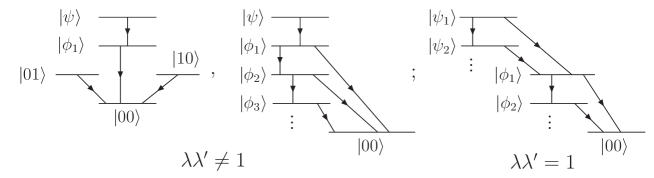
Figure 1: Four dimensional representation of ${\cal A}_{-1}$ with a composition series (50).

4.3 Four dimensional representation: $\underline{2}\otimes\underline{2}=\underline{2}\oplus\underline{2}$

In the second example, we obtain the four dimensional representation $\underline{4}$ of ${\cal A}_{-1}$ via the coproduct construction in terms of the two dimensional representation (28) of the generators $\hat{a},\hat{b},\hat{c},\hat{d}$,

$$\hat{a}|0\rangle=\lambda|0\rangle,\,\,\hat{a}|1\rangle=\lambda|1\rangle,\qquad\hat{d}|0\rangle=\lambda|1\rangle,\,\,\hat{d}|1\rangle=\lambda|0\rangle,$$

$$\hat{b}|0\rangle=\mu|1\rangle,\,\hat{b}|1\rangle=-\mu|0\rangle,\qquad\hat{c}|0\rangle=\mu|0\rangle,\,\,\hat{c}|1\rangle=-\mu|1\rangle$$ (59)

and the two dimensional representation of the generators $\hat{a}^{\prime},\hat{b}^{\prime},\hat{c}^{\prime},\hat{d}^{\prime}$ which is the same as (28) except that $\lambda,\mu$ are replaced by $\lambda^{\prime},\mu^{\prime}$. In addition, new symbols $z,\bar{z},w,\bar{w}$ are introduced,

$$z=x-iy,{\bar{z}}=x+iy,\qquad w=v-iu,{\bar{w}}=v+iu$$ (60)

where symbols $x,y,v,u$ denote the following products,

$$x=\lambda\lambda^{\prime},y=\mu\mu^{\prime},\qquad u=\lambda\mu^{\prime},v=\mu\lambda^{\prime}.$$ (61)

In this four dimensional representation $\underline{4}$, the generator $\hat{d}$ has four eigenvectors denoted by four Dirac kets $|\chi_{1}\rangle,|\chi_{2}\rangle,|\tau_{1}\rangle,|\tau_{2}\rangle$ in terms of Bell states $|\psi_{\pm}\rangle,|\phi_{\pm}\rangle$ (2) given by

$$|\chi_{1}\rangle=\frac{1}{\sqrt{2}}(|\psi_{+}\rangle+i|\phi_{+}\rangle),\qquad|\chi_{2}\rangle=\frac{1}{\sqrt{2}}(|\psi_{-}\rangle-i|\phi_{-}\rangle),$$

$$|\tau_{1}\rangle=\frac{1}{\sqrt{2}}(|\psi_{-}\rangle+i|\phi_{-}\rangle),\qquad|\tau_{2}\rangle=\frac{1}{\sqrt{2}}(|\psi_{+}\rangle-i|\phi_{+}\rangle),$$ (62)

which are related to four distinct eigenvalues of the generator $\hat{d}$,

$$\hat{d}|\chi_{1}\rangle=z|\chi_{1}\rangle,\hat{d}|\chi_{2}\rangle=-z|\chi_{2}\rangle,\qquad\hat{d}|\tau_{1}\rangle=-{\bar{z}}|\tau_{1}\rangle,\hat{d}|\tau_{2}\rangle={\bar{z}}|\tau_{2}\rangle.$$ (63)

The generator $\hat{a}$ has an eigenvalue $z$ with two degenerate eigenvectors $|\chi_{1}\rangle,|\chi_{2}\rangle$ and another eigenvalue $\bar{z}$ with two degenerate eigenvectors $|\tau_{1}\rangle,|\tau_{2}\rangle$, i.e.,

$$\hat{a}|\chi_{1}\rangle=z|\chi_{1}\rangle,\hat{a}|\chi_{2}\rangle=z|\chi_{2}\rangle,\qquad\hat{a}|\tau_{1}\rangle={\bar{z}}|\tau_{1}\rangle,\hat{a}|\tau_{2}\rangle={\bar{z}}|\tau_{2}\rangle.$$ (64)

The Dirac kets $|\chi_{1}\rangle,|\tau_{1}\rangle$ form a two-dimension cyclic representation $\underline{2}$ for the generators $\hat{b},\hat{c}$:

$$\hat{b}|\chi_{1}\rangle=-{\bar{w}}|\tau_{1}\rangle,\hat{b}|\tau_{1}\rangle=w|\chi_{1}\rangle,\qquad\hat{c}|\chi_{1}\rangle={\bar{w}}|\tau_{1}\rangle,\hat{c}|\tau_{1}\rangle=w|\chi_{1}\rangle,$$ (65)

and the Dirac kets $|\chi_{2}\rangle,|\tau_{2}\rangle$ form another two dimensional cyclic representation $\underline{2}$ given by

$$\hat{b}|\chi_{2}\rangle={\bar{w}}|\tau_{2}\rangle,\hat{b}|\tau_{2}\rangle=-w|\chi_{2}\rangle,\qquad\hat{c}|\chi_{2}\rangle={\bar{w}}|\tau_{2}\rangle,\hat{c}|\tau_{2}\rangle=w|\chi_{2}\rangle.$$ (66)

Hence we reduce the four dimensional representation $\underline{2}\otimes\underline{2}$ into the direct sum of two dimensional representations: $\underline{2}\otimes\underline{2}=\underline{2}\oplus\underline{2}$. See Figure 2 where states denoted by thick lines have the same eigenvalue and every irreducible representation $\underline{2}$ is cyclic.

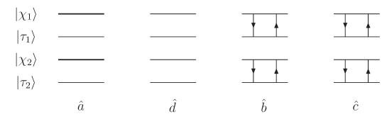
Figure 2: A four dimensional representation of ${\cal A}_{-1}$: $\underline{2}\otimes\underline{2}=\underline{2}\oplus\underline{2}$.

With the bases of $|\chi_{1}\rangle,|\chi_{2}\rangle,|\tau_{2}\rangle,|\tau_{1}\rangle$, the four dimensional representations of the generators $\hat{a},\hat{b},\hat{c},\hat{d}$ are given by the following matrices,

$$\hat{a}=\left(\begin{array}[]{cc}z&0\\ 0&{\bar{z}}\end{array}\right)\otimes 1\!\!1_{2},\qquad\hat{b}=\left(\begin{array}[]{cc}0&w\\ {\bar{w}}&0\end{array}\right)\otimes i\sigma_{y},$$ (71)

$$\hat{c}=\left(\begin{array}[]{cc}0&w\\ {\bar{w}}&0\end{array}\right)\otimes\sigma_{x},\qquad\hat{d}=\left(\begin{array}[]{cc}z&0\\ 0&{\bar{z}}\end{array}\right)\otimes\sigma_{z}.$$ (76)

These four Dirac kets $|\chi_{1}\rangle,|\chi_{2}\rangle,|\tau_{1}\rangle,|\tau_{2}\rangle$ are found to be local unitary transformations of the Bell states (2):

$$|\chi_{1}\rangle=(1\!\!1_{2}\otimes U_{1})|\psi_{+}\rangle,\qquad|\chi_{2}\rangle=(1\!\!1_{2}\otimes U_{2})|\psi_{+}\rangle,$$

$$|\tau_{1}\rangle=(1\!\!1_{2}\otimes U_{3})|\psi_{+}\rangle,\qquad|\tau_{2}\rangle=(1\!\!1_{2}\otimes U_{4})|\psi_{+}\rangle,$$ (77)

where $U_{1},U_{2},U_{3},U_{4}$ are unitary matrices given by

$$U_{1}=\frac{1}{\sqrt{2}}(1\!\!1_{2}+i\sigma_{x}),\qquad U_{2}=\frac{1}{\sqrt{2}}(\sigma_{z}-\sigma_{y}),$$

$$U_{3}=\frac{1}{\sqrt{2}}(\sigma_{z}+\sigma_{y}),\qquad U_{4}=\frac{1}{\sqrt{2}}(1\!\!1_{2}-i\sigma_{x})$$ (78)

and they form a set of complete orthonormal bases for $2\times 2$ matrices,

$$tr(U_{i}^{\dagger}U_{j})=2\delta_{ij},\qquad i,j=1,2,3,4.$$ (79)

Hence, $|\chi_{1}\rangle,|\chi_{2}\rangle,|\tau_{2}\rangle,|\tau_{1}\rangle$ are maximally entangled states like the Bell states (2) because the entangled degree of a quantum state is invariant under local unitary transformations in quantum information [1].

5 Quantum algebra associated with the $B_{+}(x)$-matrix

The $B_{\pm}(x)$-matrix (8) is obtained via Yang–Baxterization of the Bell matrix $B_{\pm}$, see [7, 8] for the detail, and it is a solution of the Yang–Baxter equation with the spectral parameter $x$. There also exists a quantum algebra from the following $\check{R}TT$ relation:

$$\check{R}(xy^{-1})(T(x)\otimes T(y))=(T(y)\otimes T(x))\check{R}(xy^{-1})$$ (80)

which is invariant under the rescaling transformation of the $\check{R}(x)$-matrix and $T(x)$-matrix by global scalar factors. Here the $\check{R}(x)$-matrix has the form of the $B_{\pm}(x)$-matrix (8) without the normalization factor. Assume the $T_{\pm}(x)$-matrix to have a formalism similar to $B_{\pm}(x)$ which is a linear combination between the Bell matrix $B_{\pm}$ (4) and its inverse $B_{\pm}^{-1}$,

$$B_{\pm}(x)=B_{\pm}+2xB_{\pm}^{-1},\qquad T_{\pm}(x)=T_{\pm}+2xT_{\pm}^{\prime},$$ (81)

where the $B_{\pm}$ matrix does not have the normalization factor $1/{\sqrt{2}}$ in (4), the $T_{\pm}$-matrix has four noncommutative operators $\hat{a},\hat{b},\hat{c},\hat{d}$ as its matrix entries and the $T_{\pm}^{\prime}$-matrix has four noncommutative operators $\hat{a}^{\prime},\hat{b}^{\prime},\hat{c}^{\prime},\hat{d}^{\prime}$ as its matrix entries. The original $\check{R}TT$ relation (80) with the spectral parameters $x,y$ is simplified into the four $\check{R}TT$ relations independent of the spectral parameter,

$$B_{\pm}(T_{\pm}\otimes T_{\pm})=(T_{\pm}\otimes T_{\pm})B_{\pm},\qquad B_{\pm}(T_{\pm}^{\prime}\otimes T_{\pm}^{\prime})=(T_{\pm}^{\prime}\otimes T_{\pm}^{\prime})B_{\pm},$$

$$B_{\pm}(T_{\pm}\otimes T_{\pm}^{\prime})=(T_{\pm}^{\prime}\otimes T_{\pm})B_{\pm},\qquad B_{\pm}(T_{\pm}^{\prime}\otimes T_{\pm})=(T_{\pm}\otimes T_{\pm}^{\prime})B_{\pm}.$$ (82)

In the following, for simplicity, we only consider the quantum algebra determined by the $\check{R}TT$ relations in terms of the $B_{+}$ matrix, $T_{+}$ matrix and $T_{+}^{\prime}$ matrix.

Obviously the generators $\hat{a},\hat{b},\hat{c},\hat{d}$ and $\hat{a}^{\prime},\hat{b}^{\prime},\hat{c}^{\prime},\hat{d}^{\prime}$ satisfy the same quantum algebra ${\cal A}_{-1}$. The algebraic equation $B_{+}(T_{+}\otimes T_{+}^{\prime})=(T_{+}^{\prime}\otimes T_{+})B_{+}$ leads to the following algebraic relations:

$$[a,a^{\prime}]=-qcc^{\prime}-q^{-1}b^{\prime}b,\qquad\{a,b^{\prime}\}=a^{\prime}b-qcd^{\prime},$$

$$\{a,c^{\prime}\}=ca^{\prime}+q^{-1}d^{\prime}b,\qquad\,\,\,\,\,[a,d^{\prime}]=cb^{\prime}-c^{\prime}b,$$

$$[b,a^{\prime}]=b^{\prime}a-qdc^{\prime},\qquad\qquad\,\,[b,b^{\prime}]=-qdd^{\prime}+qa^{\prime}a,$$

$$\{b,c^{\prime}\}=da^{\prime}-d^{\prime}a,\qquad\qquad\{b,d^{\prime}\}=db^{\prime}-qc^{\prime}a,$$

$$[c,a^{\prime}]=-ac^{\prime}-q^{-1}b^{\prime}d,\qquad\,\,\{c,b^{\prime}\}=a^{\prime}d-ad^{\prime},$$

$$[c,c^{\prime}]=q^{-1}aa^{\prime}-q^{-1}d^{\prime}d,\qquad\{c,d^{\prime}\}=c^{\prime}d+q^{-1}ab^{\prime},$$

$$[d,a^{\prime}]=b^{\prime}c-bc^{\prime},\qquad\qquad\,\,\,\,\,\,\,\,[d,b^{\prime}]=qa^{\prime}c-bd^{\prime},$$

$$[d,c^{\prime}]=d^{\prime}c+q^{-1}ba^{\prime},\qquad\qquad[d,d^{\prime}]=q^{-1}bb^{\prime}+qc^{\prime}c,$$ (83)

while the algebraic equation $B_{+}(T_{+}^{\prime}\otimes T_{+})=(T_{+}\otimes T_{+}^{\prime})B_{+}$ leads to more constraint algebraic relations:

$$[a,a^{\prime}]=q^{-1}bb^{\prime}+qc^{\prime}c,\qquad[a,b^{\prime}]=-ba^{\prime}+qd^{\prime}c,$$

$$[a,c^{\prime}]=q^{-1}bd^{\prime}+a^{\prime}c,\,\,\qquad[a,d^{\prime}]=-bc^{\prime}+b^{\prime}c,$$

$$\{b,a^{\prime}\}=ab^{\prime}-qc^{\prime}d,\,\,\,\,\,\qquad[b,b^{\prime}]=-qaa^{\prime}+qd^{\prime}d,$$

$$\{b,c^{\prime}\}=ad^{\prime}-a^{\prime}d,\,\,\,\,\,\,\,\,\qquad[b,d^{\prime}]=-qac^{\prime}+b^{\prime}d,$$

$$\{c,a^{\prime}\}=q^{-1}db^{\prime}+c^{\prime}a,\qquad\{c,b^{\prime}\}=-da^{\prime}+d^{\prime}a,$$

$$[c,c^{\prime}]=q^{-1}dd^{\prime}-q^{-1}a^{\prime}a,\,\,\,\,\,\,[c,d^{\prime}]=-dc^{\prime}-q^{-1}b^{\prime}a,$$

$$[d,a^{\prime}]=cb^{\prime}-c^{\prime}b,\qquad\qquad\{d,b^{\prime}\}=-qca^{\prime}+d^{\prime}b,$$

$$\{d,c^{\prime}\}=cd^{\prime}+q^{-1}a^{\prime}b,\qquad[d,d^{\prime}]=-qcc^{\prime}-q^{-1}b^{\prime}b.$$ (84)

The algebraic relations (5) determined by $B_{+}(T_{+}\otimes T_{+}^{\prime})=(T_{+}^{\prime}\otimes T_{+})B_{+}$ have the simplified forms:

$$[\hat{a},\hat{a}^{\prime}]=-q\hat{c}\hat{c}^{\prime}-q^{-1}\hat{b}^{\prime}\hat{b},\qquad[\hat{b},\hat{b}^{\prime}]=-q\hat{d}\hat{d}^{\prime}+q\hat{a}^{\prime}\hat{a},$$

$$[\hat{a},\hat{a}^{\prime}]=[\hat{d}^{\prime},\hat{d}],\qquad\qquad\qquad[\hat{b},\hat{b}^{\prime}]=q^{2}[\hat{c},\hat{c}^{\prime}],$$

$$\{a,b^{\prime}\}=a^{\prime}b-qcd^{\prime},\qquad\qquad[b,a^{\prime}]=b^{\prime}a-qdc^{\prime},$$

$$\{a,b^{\prime}\}=q[d,c^{\prime}],\qquad\qquad\,\,\,\,\,\,\,[b,a^{\prime}]=-q\{d^{\prime},c\}$$

$$\{\hat{a},\hat{c}^{\prime}\}=\hat{c}\hat{a}^{\prime}+q^{-1}\hat{d}^{\prime}\hat{b},\qquad\,\,\,\,[\hat{c},\hat{a}^{\prime}]=-\hat{a}\hat{c}^{\prime}-q^{-1}\hat{b}^{\prime}\hat{d},$$

$$\{\hat{a},\hat{c}^{\prime}\}=q^{-1}[\hat{d},\hat{b}^{\prime}],\qquad\qquad\,[\hat{c},\hat{a}^{\prime}]=-q^{-1}\{\hat{b},\hat{d}^{\prime}\}$$

$$[\hat{a},\hat{d}^{\prime}]=\hat{c}\hat{b}^{\prime}-\hat{c}^{\prime}\hat{b},\qquad\qquad\,\,\{\hat{b},\hat{c}^{\prime}\}=\hat{d}\hat{a}^{\prime}-\hat{d}^{\prime}\hat{a},$$

$$[\hat{a},\hat{d}^{\prime}]=[\hat{a}^{\prime},\hat{d}],\qquad\qquad\,\,\,\,\,\,\,\,\{\hat{b},\hat{c}^{\prime}\}=\{\hat{c},\hat{b}^{\prime}\}$$ (85)

and those algebraic relations (5) from $\check{R}(T_{+}^{\prime}\otimes T_{+})=(T_{+}\otimes T_{+}^{\prime})\check{R}$ can be also simplified,

$$[\hat{a},\hat{a}^{\prime}]=q^{-1}\hat{b}\hat{b}^{\prime}+q\hat{c}^{\prime}\hat{c},\qquad[\hat{b},\hat{b}^{\prime}]=-q\hat{a}\hat{a}^{\prime}+q\hat{d}^{\prime}\hat{d},$$

$$[\hat{a},\hat{a}^{\prime}]=[\hat{d}^{\prime},\hat{d}],\qquad\,\,\,\,\,\,\,\qquad[\hat{b},\hat{b}^{\prime}]=q^{2}[\hat{c},\hat{c}^{\prime}],$$

$$[\hat{a},\hat{b}^{\prime}]=-\hat{b}\hat{a}^{\prime}+q\hat{d}^{\prime}\hat{c},\qquad\,\,\{\hat{a}^{\prime},\hat{b}\}=\hat{a}\hat{b}^{\prime}-q\hat{c}^{\prime}\hat{d},$$

$$[\hat{a},\hat{b}^{\prime}]=q\{\hat{d},\hat{c}^{\prime}\},\qquad\qquad\{\hat{a}^{\prime},\hat{b}\}=q[\hat{d}^{\prime},\hat{c}],$$

$$[\hat{a},\hat{c}^{\prime}]=q^{-1}\hat{b}\hat{d}^{\prime}+\hat{a}^{\prime}\hat{c},\qquad\{\hat{c},\hat{a}^{\prime}\}=q^{-1}\hat{d}\hat{b}^{\prime}+\hat{c}^{\prime}\hat{a},$$

$$[\hat{a},\hat{c}^{\prime}]=q^{-1}\{\hat{d},\hat{b}^{\prime}\},\qquad\,\,\,\,\,\{\hat{c},\hat{a}^{\prime}\}=-q^{-1}[\hat{b},\hat{d}^{\prime}],$$

$$[\hat{a},\hat{d}^{\prime}]=-\hat{b}\hat{c}^{\prime}+\hat{b}^{\prime}\hat{c},\qquad\,\,\,\,\,\,\{\hat{b},\hat{c}^{\prime}\}=\hat{a}\hat{d}^{\prime}-\hat{a}^{\prime}\hat{d},$$

$$[\hat{a},\hat{d}^{\prime}]=[\hat{a}^{\prime},\hat{d}],\qquad\qquad\,\,\,\,\,\{\hat{b},\hat{c}^{\prime}\}=\{\hat{c},\hat{b}^{\prime}\}.$$ (86)

After some further algebraic reductions, two types of generators $\hat{a},\hat{b},\hat{c},\hat{d}$ and $\hat{a}^{\prime},\hat{b}^{\prime},\hat{c}^{\prime},\hat{d}^{\prime}$ of the quantum algebra ${\cal B}_{-1}$ are found to satisfy commutative relations,

$$\hat{a}\hat{a}^{\prime}=\hat{a}^{\prime}\hat{a},\qquad\hat{d}\hat{d}^{\prime}=\hat{d}^{\prime}\hat{d},\qquad\hat{b}\hat{b}^{\prime}=\hat{b}^{\prime}\hat{b},\qquad\hat{c}\hat{c}^{\prime}=\hat{c}\hat{c}^{\prime},$$

$$\hat{a}\hat{b}^{\prime}=\hat{a}^{\prime}\hat{b},\qquad\hat{b}^{\prime}\hat{a}=\hat{b}\hat{a}^{\prime},\qquad\hat{d}^{\prime}\hat{c}=\hat{d}\hat{c}^{\prime},\qquad\hat{c}\hat{d}^{\prime}=\hat{c}^{\prime}\hat{d}$$

$$\hat{a}\hat{c}^{\prime}=\hat{a}^{\prime}\hat{c},\qquad\hat{c}^{\prime}\hat{a}=\hat{c}\hat{a}^{\prime},\qquad\hat{b}\hat{d}^{\prime}=\hat{b}^{\prime}\hat{d},\qquad\hat{d}\hat{b}^{\prime}=\hat{d}^{\prime}\hat{b},$$

$$\hat{a}^{\prime}\hat{d}=\hat{a}\hat{d}^{\prime},\qquad\hat{d}\hat{a}^{\prime}=\hat{d}^{\prime}\hat{a},\qquad\hat{b}\hat{c}^{\prime}=\hat{b}^{\prime}\hat{c},\qquad\hat{c}\hat{b}^{\prime}=\hat{c}^{\prime}\hat{b},$$ (87)

and additional algebraic relations similar to those (18) determining ${\cal A}_{-1}$,

$$\hat{a}^{\prime}\hat{a}=\hat{d}\hat{d}^{\prime},\,\,\hat{a}\hat{d}^{\prime}=\hat{d}^{\prime}\hat{a},\,\,\hat{b}\hat{b}^{\prime}=-q^{2}\hat{c}^{\prime}\hat{c},\,\,\hat{b}\hat{c}^{\prime}=-\hat{c}^{\prime}\hat{b},\,\,\hat{a}^{\prime}\hat{b}=q\hat{d}^{\prime}\hat{c},\,\,\hat{b}\hat{a}^{\prime}=-q\hat{c}\hat{d}^{\prime},$$ (88)

where the quantum algebra determined by theses relations is called the algebra ${\mathcal{B}}_{-1}$ and the deformation parameter $q$ is irrelevant due to the rescaling transformation: $q\hat{c}\to\hat{c}$ and $q\hat{c}^{\prime}\to\hat{c}^{\prime}$. Explicitly, further research will be needed to discover interesting algebraic structures underlying the quantum algebra ${\cal B}_{-1}$.

6 Concluding remarks and problems

In this paper, we derive the quantum algebra ${\cal A}_{-1}$ using the $FRT$ construction of the Bell matrix, and list its two dimensional representations and pick up two characteristic examples for its four dimensional representations. The first example has a composition series over the complex field $\mathbb{C}$ and the second leads to $\underline{2}\otimes\underline{2}=\underline{2}\oplus\underline{2}$ which is not true for the representation of the Lie algebra [18]. In addition, we have the quantum algebra determined by the $\check{R}TT$ relation of Yang–Baxterization of the Bell matrix.

Besides these topics in the present paper and [13, 23], there still remain a series of problems to be solved in the project of exploring algebraic structures associated with the Bell matrix. In view of known achievements in quantum groups [18], readers are invited to study the following problems:

1. Does ${\cal A}_{-1}$ have a center like the quantum determinant [18] and a four-dimension representation: $\underline{2}\otimes\underline{2}=\underline{1}\oplus\underline{3}$?
   

2. The construction of universal $\check{R}$-matrix [18] in terms of generators of ${\cal A}_{-1}$.
   

3. Interesting algebraic structures underlying ${\cal B}_{-1}$ such as the quantum double.
   

4. New quantum algebras obtained by exploiting methodologies for the Sklyanin algebra [15, 16] to the Bell matrix.
   

5. Physical realization of ${\cal A}_{-1}$ (or ${\cal B}_{-1}$) and its application.
   

Note added. After this paper is submitted into the web, the authors are informed that the quantum algebra (3) has been already presented by Arnaudon, Chakrabarti, Dobrev and Mihov, see [24, 25, 26] which study the exotic bialgebras obtained by the $FRT$ recipe on the non-triangular non-singular $R$-matrix in view of the classification of the constant Yang–Baxter solution by Hietarinta [27]. As the authors of [24, 25, 26] have admitted during email correspondences between two groups, our research is completely independent of [24, 25, 26]. Here it is still necessary to make essential differences clear between both research projects. (1) Motivations. The articles [24, 25, 26] aim to finalize the explicit classification of the matrix bialgebras generated by four elements. This paper is completely motivated by the recent study of quantum information [5, 6, 7, 8, 9, 10], and it sheds a light on the connection between quantum information and quantum groups, therefore it suggests a new interdisciplinary field which can be appreciated by the community of quantum groups. (2) Quantum algebras. The articles [24, 26] use the $RTT$ relation to derive the quantum algebra called $S03$ and our paper exploits $\check{R}TT$ relation to obtain the quantum algebra ${\cal A}_{-1}$. The $\check{R}$-matrix in the present paper is called the Bell matrix which is a unitary braid representation, but the $R$-matrix [24, 25, 26] can not be called the Bell matrix since it is not a solution of the braided Yang–Baxter equation. Also, the $\check{R}$-matrix has the deformation parameter $q$ and ${\cal A}_{-1}$ is proved to be independent of $q$. Furthermore, ${\mathcal{A}}_{-1}$ is determined by six algebraic relations but $S03$ [24, 26], derived from the $RTT$ relation, has eight algebraic equations. In this sense, we actually have a “new” quantum algebra ${\cal A}_{-1}$ which has the quotient algebra $S03$. (3) Representations. It is not very easy to compare representations of quantum algebras given by [24, 25, 26] and the present paper due to the fact that the style, language and notation taken by both groups are very different. The article [24] shows representations of the dual bialgebra $s03$ of $S03$ instead of representations of $S03$. Our paper presents almost all two dimensional representations of ${\cal A}_{-1}$. More essentially, the article [24] focuses on the representation theory of the dual bialgebra $s03$ but ours is looking for interesting algebraic structures in the representation theory of ${\cal A}_{-1}$. For example, we have obtained composition series, $\underline{2}\otimes\underline{2}=\underline{2}\oplus\underline{2}$, cyclic representations, and a representation formed by four maximally entangled states which are local unitary transformations of Bell states. (4) $FRT$ dual algebra. The article [25] derives the $FRT$ bialgebra $s03_{F}$ of $S03$ and gives its representations instead of representations of $S03$. The present paper also obtains the $FRT$ dual algebra without studying its representations. But these algebraic relations are not completely the same which both groups exploit to derive the $FRT$ dual algebra. Besides calculation detail, we show the algebraic relations defining the $FRT$ dual algebra in a clear way, find the mixed algebraic relations similar to those determining ${\cal A}_{-1}$ and denote this algebra by ${\cal B}_{-1}$. (5) Physical applications. The article [26] considers an exotic eight-vertex model and an integrable spin-chain model. But the present paper suggests in its introduction that the Bell matrix and its Yang–Baxterization have negative entries which can not be explained as positive (zero) Boltzman weights in statistical physics, and therefore the authors prefer physical applications of the Bell matrix, quantum algebras ${\cal A}_{-1}$ and ${\cal B}_{-1}$ to quantum information theory. For example, see [6, 7, 8, 9, 10], in quantum computation the Bell matrix $B_{+}$ ($B_{-}$) can be identified as a universal quantum gate and the permutation $P$ matrix is the swap gate, hence the $R$-matrix [24, 25, 26] can also recognized as a universal quantum gate $R=B_{+}P$ ($R=PB_{-}$). Moreover, $P$, $B_{+}$ ($B_{-}$) can generate the virtual braid group which is a natural language for topological quantum computing [23, 28], i.e., the $R$-matrix [24, 25, 26] is an element of the virtual braid group. (6) Geometry. The article [25] briefly discusses the associated noncommutative geometry with their $R$-matrix but this paper does not study it.

References

• [1] M. Nielsen and I. Chuang, Quantum Computation and Quantum Information (Cambridge University Press, 1999).
• [2] R.F. Werner, Quantum States with Einstein-Podolsky-Rosen Correlations Admitting a Hidden-Variable Model, Phys. Rev. A 40 (1989) 4277.
• [3] A.K. Ekert, Quantum Cryptography Based on Bell’s Theorem, Phys. Rev. Lett. 67 (1991) 661-663.
• [4] C.H. Bennett, G. Brassard, C. Crepeau, R. Jozsa, A. Peres and W. K. Wootters, Teleporting an Unknown Quantum State via Dual Classical and Einstein-Podolsky-Rosen Channels, Phys. Rev. Lett. 70 (1993) 1895-1899.
• [5] H.A. Dye, Unitary Solutions to the Yang–Baxter Equation in Dimension Four, Quant. Inf. Proc. 2 (2003) 117-150. Arxiv: quant-ph/0211050.
• [6] L.H. Kauffman and S.J. Lomonaco Jr., Braiding Operators are Universal Quantum Gates, New J. Phys. 6 (2004) 134. Arxiv: quant-ph/0401090.
• [7] Y. Zhang, L.H. Kauffman and M.L. Ge, Universal Quantum Gate, Yang–Baxterization and Hamiltonian. Int. J. Quant. Inform., Vol. 3, 4 (2005) 669-678. Arxiv: quant-ph/0412095.
• [8] Y. Zhang, L.H. Kauffman and M.L. Ge, Yang–Baxterizations, Universal Quantum Gates and Hamiltonians. Quant. Inf. Proc. 4 (2005) 159-197. Arxiv: quant-ph/0502015.
• [9] Y. Zhang, Teleportation, Braid Group and Temperley–Lieb Algebra. J. Phys. A: Math. Gen. 39 (2006) 11599-11622. Arxiv: quant-ph/0610148.
• [10] Y. Zhang, Algebraic Structures Underlying Quantum Information Protocols. Arxiv: quant-ph/0601050.
• [11] C.N. Yang, Some Exact Results for the Many Body Problems in One Dimension with Repulsive Delta Function Interaction, Phys. Rev. Lett. 19 (1967) 1312-1314.
• [12] R.J. Baxter, Partition Function of the Eight-Vertex Lattice Model, Annals Phys. 70 (1972) 193-228.
• [13] J. Franko, E.C. Rowell and Z.H. Wang, Extraspecial 2-Groups and Images of Braid Group Representations. Arxiv: math.RT/0503435.
• [14] L.D. Faddeev, Lectures on Quantum Inverse Scattering Method, in Nankai Lectures on Mathematical Physics, “Integrable Systems”, pp. 23-70 (World Scientific, 1987).
• [15] E.K. Sklyanin, Some Algebraic Structures Connected with the Yang-Baxter Equation. Funct. Anal. Appl. 16 (1982) 27-34.
• [16] E.K. Sklyanin, Some Algebraic Structures Connected with the Yang-Baxter Equation: Representations of Quantum Algebras. Funct. Anal. Appl. 17 (1983) 34-48.
• [17] V.V. Bajhanov, Yu. G. Stroganov, Chiral Potts Model As a Descendant of the Six-Vertex Model, in YBE in Integral Systems, Ed., M. Jimbo, pp. 673-698 (World Scientific, 1989).
• [18] C. Kassel, Quantum Groups (Spring-Verlag New York, 1995).
• [19] N.H. Jing, M.L. Ge and Y.S. Wu, New Quantum Group Associated with a ‘Nonstandard’ Braid Group Representation, Lett. Math. Phys. 21 (1991) 183.
• [20] N.Yu. Reshetikhin, L.A. Takhtadjian and L.D. Faddeev, Quantization of Lie Groups and Lie Algebras. Algebra i Analiz 1 (1989) 178-206. English transl.: Leningrad Math. J. 1 (1990) 193-225.
• [21] C. Fan and F. Y. Wu, General Lattice Model of Phase Transitions, Phys. Rev. B 2 (1970) 723-733.
• [22] B.U. Felderhof, Direct Diagonalization of the Transfer Matrix of the Zero Field Free-Fermion Model, Physica 65 (1973) 421-451.
• [23] Y. Zhang, L.H. Kauffman and R.F. Werner, Permutation and its Partial Transpose. Arxiv: quant-ph/0606005. Accepted by International Journal of Quantum Information for publication.
• [24] D. Arnaudon, A. Chakrabarti, V.K. Dobrev and S.G. Mihov, Duality and Representations for New Exotic Bialgebras, J. Math. Phys. 43 (2002) 6238-6264. Arxiv: math.QA/0206053.
• [25] D. Arnaudon, A. Chakrabarti, V.K. Dobrev and S.G. Mihov, Spectral Decomposition and Baxterisation of Exotic Bialgebras and Associated Noncommutative Geometries, Int. J. Mod. Phys. A18 (2003) 4201-4213. Arxiv: math.QA/0209321.
• [26] D. Arnaudon, A. Chakrabarti, V.K. Dobrev and S.G. Mihov, Exotic Bialgebra S03: Representations, Baxterisation and Applications, to appear in Annales Henri Poincare. Arxiv: math.QA/0601708.
• [27] J. Hietarinta, Solving the Two-Dimensional Constant Quantum Yang–Baxter Equation, J. Math. Phys. 34 (1993) 1725.
• [28] Y. Zhang, L.H. Kauffman and M.L. Ge, Virtual Extension of Temperley–Lieb Algebra. Arxiv: math-ph/0610052.