NSF-KITP-06-84

ADE and SLE

John Cardy^a,b

^aRudolf Peierls Centre for Theoretical Physics, 1 Keble Road, Oxford OX1 3NP, UK

^bAll Souls College, Oxford

October 2006

We point out that the probability law of a single domain wall separating clusters in ADE lattice models in a simply connected domain is identical to that of corresponding chordal curves in the lattice O$(n)$ and $Q$-state Potts models, for suitable $n$ or $Q$. They are conjectured to be described in the scaling limit by chordal SLE_κ with $\kappa$ rational and $>$2. However in a multiply-connected domain the laws can differ from those for the corresponding O$(n)$ or Potts model. The correspondence also sheds light on the scaling limit of multiple curves.

1 Introduction

Chordal Schramm-Loewner evolution[1] (SLE) is the unique family of conformally invariant measures on curves connecting two distinct boundary points of a simply connected domain. It is commonly conjectured (and in some cases proved) to describe the scaling limit of suitably defined curves in critical equilibrium lattice models, for example the O$(n)$ and $Q$-state Potts models. These models are originally defined as lattice spin models for integer values of $n$ and $Q\geq 2$. However in the random curve representation of either model as a gas of non-intersecting closed loops, each loop is weighted with a factor $n$ (resp. $\sqrt{Q}$) and so it gives a probability measure on loops for all non-negative values of these parameters. These measures are however non-local in the sense that they are not product measures over regions with a finite number of degrees of freedom. To get local measures, one needs to go back to the spin representations, which make sense only for $n=1,2$ and $Q=2,3,4$ in the regions $n\leq 2$ and $Q\leq 4$ where these models are conjectured to have a non-trivial scaling limit.

The importance of a local probability measure arises in the connection with conformal field theory (CFT), because it implies that the corresponding CFT should satisfy reflection positivity and therefore be representable in terms of operators acting on a space of states with non-negative norm. In any 2d CFT, the scaling operators may be arranged into representations of two commuting Virasoro algebras, and the above requirement then implies that these representations be unitary. This fact was used by Friedan, Qiu and Shenker[2] to classify all such possible unitary CFTs with central charge $c<1$. This leads to a discrete series of possible values for $c$

$$c=1-\frac{6}{m(m+1)}$$

with $m$ an integer $\geq 3$, while the allowed values of the scaling dimensions $(h,\bar{h})$ (conformal weights) of the primary operators are restricted to take values in the Kac table

$$h_{r,s}=\frac{\big{(}r(m+1)-sm\big{)}^{2}-1}{4m(m+1)}$$

where $1\leq r\leq m-1$, $1\leq s\leq m$.

One important feature of these CFTs is the closure of the operator product expansion (OPE) on a finite number of primary operators or their descendants, with scaling dimensions within the Kac table above. This also happens in a wider class of models, the minimal models, which are labeled by a coprime pair of positive integers $(p,p^{\prime})$, with the formulae above replaced by

$$c=1-\frac{6(p-p^{\prime})^{2}}{pp^{\prime}}$$ (1)

and

$$h_{r,s}=\frac{(rp-sp^{\prime})^{2}-(p-p^{\prime})^{2}}{4pp^{\prime}}$$

where $1\leq r\leq p^{\prime}-1$, $1\leq s\leq p-1$.

However this result does not determine exactly which of these values occur in a given CFT. It was pointed out[3] that this is highly constrained by modular invariance of the partition function on the torus. This condition was solved by Cappelli, Itzykson and Zuber[4], who showed that the resulting CFTs can be labelled by Coxeter diagrams[5] of type A, D or E with Coxeter number $p$. By generalizing the restricted solid-on-solid models of Andrews, Baxter and Forrester[6] (which correspond to the A series) Pasquier[7, 8] constructed lattice ADE models, with local weights defined by the adjacency matrix of G, which he showed, on the basis of Coulomb gas and other arguments, give the CFTs corresponding to $p^{\prime}<p$. Later, Kostov[9] defined dilute ADE models which correspond to the other case.

In this note we recall these arguments in the context of identifying candidates for curves in lattice models with local weights which should have SLE as their scaling limit. In the case of a simply connected domain with suitable boundary conditions, we argue that these curves have weights identical with those of the O$(n)$ or $Q$-state Potts models with the same value of $c$, and therefore if the latter converge to SLE in the scaling limit, so do the corresponding curves in the ADE models. For other geometries, however, the weights are not in general the same, even in the scaling limit. This observation relates to the apparent non-uniqueness of attempted definitions of SLE in multiply-connected domains, and of connection probabilities of multiple SLEs. We also show that, in the case A_m, the law of $N<m$ curves is the same as $N$ ‘ordinary’ multiple SLEs (with the same value of $\kappa$) conditioned not to meet. In that case the resulting partition functions agree with those recently proposed by Bauer, Bernard and Kytola[10] and Dubédat[11].

Most of the ideas in this paper are not new, in fact some of them date back 20 years. The main purpose to recall them in the context of SLE for those currently working in this active field.

The outline of this paper is as follows. In Sec. 2 we define the dilute and non-dilute models for which the heights take values on the nodes of any connected graph $\cal G$. We recall the arguments of Pasquier which show that the can be reformulated as a gas of non-intersecting loops, where each loop is weighted by $\Lambda$, an eigenvalue of the adjacency matrix of $\cal G$. For the local weights in these models to be real and positive, $\Lambda$ must be the largest eigenvalue. The requirement that this weight should be strictly less than than 2 (corresponding to CFTs with $c<1$) then restricts $\cal G$ to be one of the ADE Coxeter diagrams. Inclusion of $\Lambda=2$ ($c=1$) allows $\cal G$ to be an extended Coxeter diagram of type $\hat{\rm A}$, $\hat{\rm D}$, $\hat{\rm E}$, or A_∞, which is the discrete gaussian model. The other non-unitary minimal models then correspond to taking $\Lambda$ to be a non-maximal eigenvalue. In general these have complex local weights, although the loop gas measure still makes sense as long as $\Lambda\geq 0$.

In a simply connected domain with homogeneous boundary conditions, there are only closed loops, and Pasquier’s arguments show that in any of the ADE models these are weighted exactly as in the corresponding O$(n)$ or $Q$-state Potts models, and therefore should have the same scaling limit. This has recently been conjectured to be the Conformal Loop Ensemble (CLE_κ)[12]. The above identification of ADE and the other models is in agreement with the idea that, given a value of $\kappa$, the CLE is a unique conformally invariant measure on nested closed loops in a simply connected domain.

In Sec. 3 we identify the clusters whose boundaries are supposed to be described by SLE in the scaling limit. In the dilute ADE model, these are clusters of adjacent lattice sites with the same height. In the non-dilute model they are boundaries of clusters in a Fortuin-Kasteleyn-type representation. By trivially extending Pasquier’s arguments we show how, with suitable boundary conditions, chordal curves separating clusters whose heights correspond to adjacent nodes of $\cal G$ have the same weights as corresponding curves in the O$(n)$ and Potts models. Then, in Sec. 4 we discuss the additional features which arise for multiple curves and in multiply-connected domains.

After this work was completed a paper[13] by P. Fendley appeared which covers some of the same material from a slightly different point of view. In addition this paper discusses new loop models corresponding CFTs with central charge $c>1$ which would be very interesting to understand from the SLE perspective.

2 ADE lattice models and loop gases.

In this section we recall the definition of the local height model associated with a graph $\cal G$, and the arguments of Pasquier[8] transforming it to a loop gas.

2.1 Dilute ADE models.

This case is actually slightly simpler to discuss, so we present it first. The dilute models were first introduced by Kostov[9] (see also Nienhuis[14]), and shown to be part of an integrable family of models satisfying the Yang-Baxter relations by Roche[15] and by Warnaar, Nienhuis and Seaton[16]. Kostov’s models were originally defined on a square lattice, but it is more natural, and symmetrical, to define them on a regular triangular lattice as follows.

At each site $j$ of the triangular lattice is a height $h_{j}$, which takes values on the nodes of a fixed connected graph $\cal G$. We denote the adjacency matrix of $\cal G$ by $\bf G$. There is a constraint whereby the heights at neighboring sites of the triangular lattice must either be equal, or adjacent on $\cal G$. Assuming that $\cal G$ has no cycles of length $\leq 3$, this implies that at least two of the heights around any elementary triangle must be equal. The weight for a given configuration is the product of the weights over all the elementary triangles of the lattice. These are given as follows: if all the heights are equal, the weight is 1; if the heights are, for example, $(a,b,b)$, the weight is $x(S_{a}/S_{b})^{1/6}$, where $S_{a}$ is a strictly positive function on the nodes of $\cal G$, to be made explicit later.

Figure 1: An elementary triangle with unequal heights $(a,b,b)$ is marked by a curve segment on the dual honeycomb lattice as shown. This carries a weight $(S_{a}/S_{b})^{1/6}$.

In the second case, one may mark the triangle as shown in Fig. 1 by two straight lines connecting the midpoints of the two edges joining the heights which differ to the center of the triangle. These must join up with similar lines in the neighboring triangles, and therefore must form closed, non-intersecting, loops on the dual honeycomb lattice (or open curves which end at a boundary.) For the time being, restrict to a simply connected domain where all the heights on the boundary are fixed to take the same value. Then we have only closed loops. Every loop separates a cluster of sites all with the same height, say $a$, on its immediate interior from a cluster of sites with a different height, say $b$, adjacent to $a$ on $\cal G$, on its exterior. If one multiplies all the factors of $(S_{a}/S_{b})^{\pm 1/6}$ around a given loop, this always gives $S_{a}/S_{b}$ irrespective of the shape of the loop.

The loops form a nested structure. Now sum over all allowed values of the heights consistent with a given configuration of loops, starting with the innermost clusters. Each sum has the form

$$\sum_{a}G_{ab}(S_{a}/S_{b})$$

It is only straightforward to repeat this procedure at the next level of nesting if this is some constant $\Lambda$ independent of $b$: or, equivalently

$$\sum_{a}G_{ab}S_{a}=\Lambda S_{b}$$

That is, the $S_{a}$ should be the components of an eigenvector of $\bf G$ with eigenvalue $\Lambda$. Taking this to be the largest (Perron-Frobenius) eigenvalue then guarantees that all the $S_{a}$ are positive.

Summing iteratively over all heights of all the clusters then gives a factor $\Lambda$ for each closed loop. This is to be compared with the O$(n)$ model on the honeycomb lattice, which can be written in terms of identical loops weighted with a factor $n$ for each loop, as well as a factor $x$.

This result shows that the law of the dilute ADE loops in a simply connected domain with homogeneous fixed height boundary conditions is identical to those of the $O(n)$ model with free boundary conditions, at the same value of $x$, with the identification $n=\Lambda$. If $n>2$, the O$(n)$ model is known either to be non-critical or to exhibit only first-order critical behavior. The condition that $\Lambda<2$ restricts $\cal G$ to be of the ADE type (or ${\rm A}_{2m}/{\rm Z}_{2}$, which does not give a sensible model.) $\Lambda=2$ corresponds to one of the extended ADE diagrams or A_∞. In each of the ADE cases, $\Lambda=2\cos(\pi/h)$ where $h$ is the Coxeter number of the graph.

The case A_m is simple: we then have $\Lambda=2\cos(\pi/(m+1))$ and $S_{a}\propto\sin(\pi a/(m+1))$ with $a\in\{1,\ldots,m\}$. The case $m=2$ corresponds to the Ising model on the triangular lattice.

The O$(n)$ model for $n\leq 2$ on the honeycomb lattice is conjectured[17] to have a critical point at $x=x_{c}=(2+\sqrt{2-n})^{-1/2}$. The scaling limit is also conjectured, using Coulomb gas and CFT arguments, to correspond to $\kappa\leq 4$ where $n=-2\cos(4\pi/\kappa)$. Putting these relations together in our case we have

$$\kappa=\frac{4h}{h+1}$$

where $h=m+1$ for the A_m models.

The complete set of eigenvalues of $\bf G$ are given by $\Lambda=2\cos(\pi h^{\prime}/h)$ where $h^{\prime}<h$ is one of the Coxeter exponents of $\cal G$: for A_m these take all integer values in the range $1\leq h^{\prime}\leq m$. The generalization of the above relation is then

$$\kappa=\frac{4h}{h+h^{\prime}}$$ (2)

If we consider all possible A_m models with $m\geq 2$, this includes all rational values of $\kappa$ in the interval $(2,4)$. However only those in $(\frac{8}{3},4)$ have positive weights for the loops.

The whole phase for $x>x_{c}$ is supposed be critical and corresponds to $\kappa\geq 4$, with the same relation between $n$ and $\kappa$. In that case we have, in the unitary case,

$$\kappa=\frac{4h}{h-1}$$

and more generally

$$\kappa=\frac{4h}{h-h^{\prime}}$$ (3)

If we consider all possible A_m models, this includes all rational values of $\kappa>4$. However only those in $(4,8)$ have positive weights for the loops.

2.2 Non-dilute ADE models.

These are most easily defined on a square lattice. Once again there are heights at the vertices which take values on the nodes of $\cal G$, but now heights at neighboring sites must be strictly adjacent on $\cal G$ and are not allowed to be equal. If $\cal G$ has no cycles of length $\leq 4$, this implies that at least one of the diagonally opposite pairs of heights in each elementary square must be equal. In any case, this constraint is enforced by the weights (see below). Note that this also implies that the even sublattice is populated by heights from the even nodes of $\cal G$, and the odd sublattice by heights from the odd nodes (or vice versa, as determined by the boundary conditions.) The weight for a height configuration on the whole lattice is a product of the weights around each elementary square.

Figure 2: Heights around an elementary square. If the first term in (4) is chosen, an edge is drawn connecting $a$ and $c$ as shown. This carries weight $(S_{b}S_{d}/S_{a}^{2})^{1/4}$, which can be distributed into factors $(S_{b}/S_{a})^{1/4}$ and $(S_{d}/S_{a})^{1/4}$ at the corners of the corresponding loop(s) on the medial lattice.

Labelling the heights by $(a,b,c,d)$ (see Fig. 2), these are given by

$$W(a,b,c,d)=\left(\frac{S_{b}S_{d}}{S_{a}S_{c}}\right)^{1/4}\,\delta_{ac}+\left(\frac{S_{a}S_{c}}{S_{b}S_{d}}\right)^{1/4}\,\delta_{bd}$$ (4)

The weight for a given configuration on the whole lattice may now be expanded as a sum of $2^{N}$ terms, where $N$ is the total number of elementary squares. In each elementary square we may draw an edge connecting the sites with heights $a$ and $c$ if the first term is chosen, or one connecting the sites with heights $b$ and $d$ if the second term is chosen. The result is to decompose the edges of the even sublattice into clusters. Within each cluster all the heights are constrained to be equal. A similar decomposition holds for the edges of the odd sublattice. Neighboring clusters on the even sublattice are separated by clusters on the odd sublattice and vice versa. The picture is identical to that which occurs in the Fortuin-Kasteleyn (random cluster) representation of the Potts model, with the clusters on the even sublattice being identified as the clusters of Potts spins, while those on the odd sublattice correspond to the clusters of dual spins. As in the Potts case, neighboring clusters can be separated by dense non-intersecting curves on the medial lattice, which either form closed loops or end at a boundary.

The nice property of this picture is that the weights can now be distributed at the corners of these curves (see Fig. 2). A corner which separates a cluster of height $b$ from one of height $a$, such that the height within the acute angle of the corner is $b$, carries a weight $(S_{b}/S_{a})^{1/4}$.

Now consider a simply connected domain with homogeneous wired boundary conditions. By wired we mean that the squares on the boundary carry only the term in (4) which corresponds to there being an edge between the boundary sites. (Clearly this requires that all the boundary sites be on the same sublattice, say even.) We can then suppose that the heights on the boundary are fixed to a given value. The edges connected to the boundary form the boundary cluster. This cluster may be adjacent on its interior to several clusters on the odd sublattice, which themselves may be adjacent on the interior to clusters on the even sublattice, and so on. The curves on the medial sublattice may only form closed loops. Each loop may touch only one cluster internally, and one externally. The loops form a nested structure as in the dilute case, separating clusters on which the heights all agree. A loop enclosing a cluster of height $a$ and enclosed by one of height $b$ carries a total weight $(S_{a}/S_{b})$, irrespective of the shape of the loop.

The summation over the heights for a given configuration of loops then proceeds as in the dilute case. The weighting of the loops is exactly as for the FK representation of the critical $Q$-state Potts model, with identification $\Lambda=\sqrt{Q}$. The scaling limit for $\Lambda\leq 2$ is supposed to be described by CLE_κ as before. In this case we get only values of $\kappa\geq 4$, however, corresponding to the values in (3). Now the case ${\cal G}={\rm A}_{3}$ corresponds to the Ising model. The heights on one sublattice are all fixed to the same value $a=2$. On the other sublattice they take the values $(1,3)$ corresponding to $\pm 1$ in the usual formulation of the Ising model. The $Q$-state Potts model in fact corresponds to $\cal G$ being a star graph with a central node connected to $Q$ points. It is straightforward to check that the largest eigenvalue of the adjacency matrix is $\Lambda=\sqrt{Q}$.

It is interesting to attempt to identify the boundaries of connected clusters with the same value of the height variables in the non-dilute ADE models (as for the Ising model.) For the $A_{m}$ models some progress can be made in that direction. Consider the elementary squares around which the heights take the values $(a,a+1,a,a-1)$. If we draw an edge connecting the two sites with height $a$, this may be thought of as part of the boundary separating clusters of heights $a\pm 1$. It is straightforward to see that only an even number of these edges can meet at any one vertex of the square lattice, and therefore the set of such cluster boundaries is the same as in the Ising case $m=3$. However, to proceed further, one needs to sum over all possible values of the heights within each closed loop, and this is difficult is general. At the critical point, we expect to recover weights for the loops which are the same as those in the dilute O$(n)$ model on the square lattice (with some convention for dealing with the vertices where 4 edges meet) but it may be that this identification occurs only in the scaling limit. In the next section we present some evidence for this conjecture.

2.3 Models with $\kappa=4$.

The models defined on graphs $\cal G$ whose adjacency matrix has largest eigenvalue $\Lambda=2$ correspond to $\kappa=4$. In that case $\cal G$ is either A_∞ (the integers) or one of the extended Coxeter diagrams, for example $\hat{\rm A}_{m}$. This has $m$ nodes arranged in a ring. The first case corresponds to the ordinary solid-on-solid model with the constraint that nearest neighbor height differences take the values $(0,\pm 1)$ (dilute model) or strictly $(\pm 1)$ (non-dilute model). The $\hat{\rm A}_{m}$ models are particular realisations of the ${\mathbb{Z}}_{m}$ clock models, with same nearest-neighbor constraints. In these cases the largest eigenvalue of the adjacency matrix is always $\Lambda=2$, corresponding to $S_{a}={\rm const.}$, and the arguments of the previous sections show that the law of loops (and chordal curves – see below) in a simply connected domain is identical with that of the O$(2)$ model (dilute) or the FK 4-state Potts model (non-dilute). (The latter in fact corresponds exactly to $\hat{\rm D}_{3}$.) However in the clock models it is necessary that $m\geq 4$, to avoid 3-cycles. All these models are supposed to have the same scaling limit given by the gaussian free field.

3 Inhomogeneous boundary conditions and chordal curves.

In this section we identify curves in these models which are candidates for chordal SLE in the scaling limit. We show that the law of these curves is identical to those in the corresponding O$(n)$ and Potts models.

The dilute ADE models are simpler to discuss. To identify a chordal curve we consider a simply connected domain and impose one type of fixed boundary condition, say $a$, on one segment of the boundary (the left boundary), and another, say $b$, on its complement (the right boundary). This is strictly possible only if $a$ and $b$ are adjacent on $\cal G$, in which case, in the construction above, there is exactly one lattice curve $\gamma$ connecting the points $z_{1}$, $z_{2}$ where the boundary conditions change. The sites immediately to the left of $\gamma$ all have height $a$; those immediately to its right have height $b$. If $a$ and $b$ are not adjacent on $\cal G$, there must be several lattice sites separating the left and right parts of the boundary. This interval will go to a point in the scaling limit, but the sites in between will be the starting points of more than one curve. This situation therefore cannot give a single chordal curve – the right hand boundary of the height cluster connected to the left boundary is not identical with the left boundary of the cluster connected to the right boundary.

Given now a chordal curve $\gamma$ connecting $z_{1}$ and $z_{2}$, as well as sets of nested closed loops in the simply connected domains (with homogeneous boundary conditions) to its left and right, we may sum over all the heights as before, beginning with the most deeply nested clusters. This will give rise, as before, to a factor $\Lambda$ for each closed loop. The curve $\gamma$ itself will accumulate factors $(S_{a}/S_{b})^{\pm 1/6}$ for each left or right turn. However since the number of right minus the number of left turns is the same for every configuration, the relative weights are all the same.

We conclude that the law of a single chordal curve in the dilute ADE models in a simply connected domain is the same as in the O$(n)$ model, and is therefore conjectured, in the scaling limit, to be given by SLE_κ with $\kappa$ given by (3,2).

For the non-dilute ADE models in the FK representation, consider boundary conditions wired to a fixed height $a$ on the left boundary, and to height $b$ on the right boundary. Once again, the right boundary of the cluster attached to the left boundary, and the left boundary of the cluster attached to the right boundary, are adjacent only if $a$ and $b$ are adjacent on $\cal G$. (Note that this means that the sites on the left and right boundaries must be on opposite sublattices.) This then defines a chordal lattice curve $\gamma$ which separates these two clusters. The summation over heights goes as before, and we conclude that the law of $\gamma$ is identical to the law of the curve in the $Q$-state Potts model, for the appropriate $Q$, with wired boundary conditions on the Potts spins on the left boundary and free boundary conditions (i.e. wired on the dual spins) on the right boundary, which touches the right boundary of the FK cluster attached to the left boundary. This is supposed to be given by SLE_κ in the scaling limit, with $\kappa\geq 4$.

In this case, there is supporting evidence for this identification from CFT. In the A_m models, the boundary changing operator between a boundary wired to height $1$ and to height $a$ was identified by Saleur and Bauer[18] as a $\phi_{1,a}$ operator in the Kac classification. Here $1$ is a height at either extremity of the diagram. According to boundary CFT, the operator content at a change of boundary conditions from $a$ to $b$ is given by fusing $\phi_{1,a}$ and $\phi_{1,b}$. According to the fusion rules of the A theories, this contains a $\phi_{1,2}$ operator if and only if $a$ and $b$ are adjacent on the diagram. As was shown by Bauer and Bernard, and Friedrich and Werner, the existence of a $\phi_{1,2}$ boundary condition changing operator is necessary for this to be an end point of an SLE (with $\kappa\geq 4$.)

A similar argument may be applied to the height cluster boundaries in the non-dilute case. Saleur and Bauer[18] also considered boundary conditions where the heights are fixed to $r$ on the boundary sites, and to $r+1$ on the sites adjacent to the boundary, and argued that the the boundary condition changing operator between $(1,2)$ and general $(r,r+1)$ corresponds to $\phi_{r,1}$ in the Kac classification. The fusion rules can then be used to show that the leading boundary condition changing operator between boundary conditions $a,a-1$ and $a,a+1$ is a Kac $\phi_{2,1}$ operator, which is a necessary condition for there to be an SLE with $\kappa<4$ starting at the point where the boundary condition changes. A candidate for this curve is the cluster boundary described in the previous section, with some convention for dealing with the 4-valent vertices.

It was recently shown by Riva and Cardy[19] and Smirnov[20] that parafermionic observables of fractional spin $s$ may be defined on the curves in FK Potts models which weight the indicator function that curve goes along a given edge of the medial lattice with a phase $e^{is\theta}$, where $\theta$ is the winding angle. These observables are discrete holomorphic if $\kappa=8/(s+1)$. (Smirnov has also given a similar construction for the O$(n)$ model.) Their correlators should converge to those of holomorphic parafermions in the corresponding CFT, although the convergence has so far been proved[20] only for the Ising case. The above result then implies that holomorphic parafermions of spin $s=1\pm(2h^{\prime}/h)$ should also exist in the ADE models.

4 Non-simply connected domains and multiple SLEs

4.1 Non-simply connected domains

In this section we show that the law of chordal curves in a multiply-connected domain can in general be different for different models with the same value of $\kappa$. As an example, consider the annulus pictured as a simply connected domain with a hole, and a chordal curve $\gamma$ which connects two point on the same boundary of the annulus (see Fig. 3). In the ADE models, this can be enforced by imposing fixed height boundary conditions, say $a$ and $b$, on the left and right segments of the other boundary, and $c$ (not equal to $a$ or $b$) in the inner boundary. In the Potts model, it would be necessary to condition $\gamma$ not to hit the inner boundary. Without loss of generality we may assume the $\gamma$ passes to the left of the hole, so that the region to its right has the topology of an annulus.

Figure 3: A chordal curve in the annulus connecting two points on the same boundary. The law of the this curve is sensitive to the number of non-contractible loops, whose weights depend non-trivially on the boundary heights.

In this case, as well as the chordal curve, there will in general be non-contractible closed loops which wrap around the annulus, as well as loops homotopic to a point. The summation over the heights within the latter proceeds as before, giving a factor $\Lambda$ for each loop. However this is is not the case for the non-contractible loops. In fact, if there are $N$ such loops, we get instead

$$\left[{\bf G}^{N}\right]_{bc}$$ (5)

which may be interpreted as the number of $N$-step random walks on $\cal G$ from $b$ to $c$. In general this depends on the choice of $\cal G$ and on where $b$ and $c$ are located on $\cal G$. For the Potts model, on the other hand, there is always simply a factor $(\sqrt{Q})^{N}$, essentially because all the other relevant eigenvalues of $\cal G$ are zero.

This result implies that there is no unique way of prescribing the driving term for SLE in an annulus or more complicated multiply-connected domain (although we note that this difficulty does not arise for curves which begin and end on different boundaries of the annulus.) The distribution of the random variable $N$ depends on the modulus of the annulus and can be computed using Coulomb gas methods. It would be interesting to use this to compute the SLE driving term for each of these models.

However we note that there is nevertheless a ‘canonical’ version, in which each non-contractible loop is counted with a weight $\Lambda$. In the ADE models this may be realised by summing over the boundary conditions $c$ on the inner boundary, and weighting them with a factor $S_{c}$. This projects out the required eigenvalue.

Also, as the size of the hole shrinks, keeping all other length scales fixed, the typical value of $N$ goes to infinity. In that case, only the largest eigenvalue $\Lambda$ of $\cal G$ is important in (5), and the law of $\gamma$ becomes universal once again. In this case it should be described by some version of SLE$(\kappa,\rho)$.

4.2 Multiple SLEs.

The law of multiple chordal curves in a simply connected domain has been considered by Bauer, Bernard and Kytola[10] from the point of view of CFT, and also by Dubédat[11]. One of the objects of interest is not the law of the curves themselves (which is given by a version of SLE$(\kappa,\rho)$) but the relative probabilities of the various ways the curves can connect, or arch configuration, given a set of $2N$ points on the boundary. These are given by ratios of partition functions in statistical mechanics, which satisfy second-order partial differential equations with respect to the positions of the points. These are just the BPZ equations resulting from the fact that the CFT operators which create the curves are $\phi_{1,2}$ (or $\phi_{2,1}$) operators in the Kac classification (for $\kappa>4$ and $<4$ respectively.) However there is a question of which boundary conditions correspond to a given arch configuration. A clear answer to this is given by considering the equivalent problem in the A_m models.

Figure 4: An arch configuration in which $N$ curves are conditioned to connect the boundary points a shown. Such a conditioning is natural in the A_m models if $N<m$.

Let us consider the geometry shown in Fig. 4. There are $2N$ points on the real axis, connected by $N$ curves in the upper half plane. Label these points in increasing order as $(x_{1},\ldots,x_{N})$ and $(y_{N},\ldots,y_{1})$, and consider the connection shown in Fig. ?? in which $x_{j}$ is connected to $y_{j}$. Denote the partition function for this arch configuration by $Z_{N}(x_{1},\ldots,x_{N};y_{N}\ldots,y_{1})$. Its possible behavior as neighboring points approach each other is given by the fusion rules of CFT: $\phi_{1,2}\cdot\phi_{1,2}=\phi_{1,1}+\phi_{1,3}$, which means that as $\delta=x_{j+1}-x_{j}\to 0$, $Z_{N}$ can be expressed as a linear combination of two terms, one of which behaves as $\delta^{-2h_{1,2}}=\delta^{-(6-\kappa)/\kappa}$ and the other as $\delta^{h_{1,3}-2h_{1,2}}=\delta^{2/\kappa}$. Identical possibilities hold if $x_{N}$ approaches $y_{N}$.

Bauer, Bernard and Kytola identify an arch configuration in which $x_{1}$ is connected with $y_{1}$ as being associated with a solution where the dominant term as $x_{1}\to y_{1}$ is the fusion to the identity operator $\phi_{1,1}$, while if neighboring curves are conditioned not to meet, as for $x_{j}\to x_{j+1}$, it is associated with the solution corresponding to fusion to the $\phi_{1,3}$ operator. In that case it is natural to normalize $Z_{N}$ so that, as $x_{N}\to y_{N}$

$$Z_{N}(x_{1},\ldots,x_{N};y_{N}\ldots,y_{1})\sim(y_{N}-x_{N})^{-(6-\kappa)/\kappa}\,Z_{N-1}(x_{1},\ldots,x_{N-1};y_{N-1}\ldots,y_{1})$$

with $Z_{0}=1$ by convention.

Among all the solutions to the system of BPZ differential equations with the above boundary conditions as $x_{j}\to y_{j}$ there is in general one in which the operators $\phi_{1,2}(x_{j})$ all fuse to the $\phi_{1,N+1}$ operator, and similarly for the $\phi_{1,2}(y_{j})$. In that case it can be argued that in this limit $Z_{N}$ has the form

$$Z_{N}\propto\prod_{1\leq j<k\leq N}(x_{k}-x_{j})^{2/\kappa}\,\prod_{1\leq j<k\leq N}(y_{j}-y_{k})^{2/\kappa}\,(y-x)^{-2h_{1,N+1}}$$ (6)

where $x\sim x_{j}$, $y\sim y_{j}$.

By conformally mapping $y$ to infinity, Bauer et al[10] identify this boundary condition as selecting the partition function for $N$ curves conditioned to go to infinity (rather than forming arches among the points $x_{j}$). For small enough $N$ this is completely consistent with the identification with curves in the A_m model. Suppose in the A_m model we fix the boundary conditions on each segment of the real axis to be $(1,2,\ldots,N,N+1,N,N-1,\ldots,1)$ in order, where these integers label nodes on the Coxeter diagram. Each of the points where the boundary conditions change will be an end-point for a curve, and will correspond to a $\phi_{1,2}$ operator. As long as $N\leq m-1$, without any further conditioning these curves must connect as in Fig. 4. Moreover if we now let $x_{j}\to x$ and $y_{j}\to y$, we have boundary condition changing operators from $1$ to $N$ at $x$ and $y$, which are known[18] to correspond to $\phi_{1,N+1}$ operators.

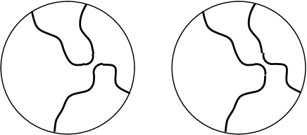
Figure 5: The two different ways two curves can connect. The relative probabilities depend not only on $\kappa$ but also on the model and the boundary conditions.

However, these boundary conditions do not specify the relative normalization of the partition functions for each arch configuration, which are needed for the connection probabilities. For example, in the case $N=2$, what are the relative probabilities of the two arch configurations shown in Fig. 5? The boundary conditions above fix each partition function as a function of the cross-ratio $\eta$ of the four points, up to overall constants. In the case of the Ising model ($\kappa=3$) or of the boundaries of the FK Potts clusters, where there is a ${\mathbb{Z}}_{2}$ symmetry (spin reversal or duality) under the exchange of the two configurations, one may argue[10] that the relative weight must be 1 at the symmetry point $\eta=\frac{1}{2}$, which the determines the relative probabilities for all values of $\eta$. However, for other ADE models with the same value of $\kappa$, this ratio may be modified. To see this it is useful to examine the case where the two curves pass through the same square (in the non-dilute models.) In that case the two different ways of connecting the curves are weighted in the ratio $(S_{a}/S_{b})^{1/2}:(S_{b}/S_{a})^{1/2}=S_{a}/S_{b}$. For the Ising or Potts models this would be unity, but in general it is different. It is also easy to see that the factor $S_{a}/S_{b}$ depends only on the topology and not the fact that the curves pass through the same square.

Once again this argument shows that certain aspects of these random curves, even in the scaling limit, are model-dependent and not solely determined by $\kappa$.

Acknowledgments. This work was carried out at the Kavli Institute for Theoretical Physics, Santa Barbara, supported in part by the National Science Foundation under Grant No. PHY99-07949, in the course of the program on Stochastic Geometry and Field Theory. I am grateful to several participants of that program, including M. Bauer, D. Bernard, G. Lawler, A. Ludwig, S. Sheffield, S. Smirnov and J.-B. Zuber for useful suggestions and critical comments, as well as to H. Saleur.

References

- [1] O. Schramm, Israel J. Math. 118, 221, 2000 (math.PR/9904022).
- [2] D. Friedan, Z. Qiu and S. Shenker, Phys. Rev. Lett. 52, 1575, 1984.
- [3] J. Cardy, Nucl. Phys. B 270, 186, 1986.
- [4] A. Cappelli, C. Itzykson and J.-B. Zuber, Comm. Math. Phys. 113, 1, 1987.
- [5] For pictures and further information, see Refs.[8, 9].
- [6] G.E. Andrews, R.J. Baxter and P.F. Forrester, J. Stat. Phys. 35, 193, 1984.
- [7] V. Pasquier, Nucl. Phys. B 285, 162, 1986.
- [8] V. Pasquier, J. Phys. A 20, L1229, 1987.
- [9] I. Kostov, Nucl. Phys. B 376, 539, 1992; hep-th/9112059.
- [10] M. Bauer, D. Bernard and K. Kytola, J. Stat. Phys. 120, 1125, 2006; math-ph/05030124.
- [11] J. Dubédat, math.PR/0411299.
- [12] S. Sheffield, math.PR/0609167.
- [13] P. Fendley, cond-mat/0609435.
- [14] B. Nienhuis, J. Phys. A 15, 199, 1982.
- [15] Ph. Roche, Phys.Lett.B 285, 49,1992; hep-th/9204036.
- [16] S.O. Warnaar, B. Nienhuis and K.A. Seaton, Phys. Rev. Lett. 69, 710, 1992.
- [17] B. Nienhuis, J. Stat. Phys. 34, 731, 1983; and in Phase Transitions and Critical Phenomena, v.11, C. Domb and J. Lebowitz, eds. (Academic, 1987).
- [18] H. Saleur and M. Bauer, Nucl. Phys. B 320, 591, 1989.
- [19] V. Riva and J. Cardy, cond-mat/0608496.
- [20] S. Smirnov, in Proceedings of the International Congress of Mathematicians (Madrid, August 22-30, 2006), European Mathematical Society, 2006, II, 1421, 2006.