Fractal Strings and Multifractal Zeta Functions

Abstract.

For a Borel measure on the unit interval and a sequence of scales that tend to zero, we define a one-parameter family of zeta functions called multifractal zeta functions. These functions are a first attempt to associate a zeta function to certain multifractal measures. However, we primarily show that they associate a new zeta function, the topological zeta function, to a fractal string in order to take into account the topology of its fractal boundary. This expands upon the geometric information garnered by the traditional geometric zeta function of a fractal string in the theory of complex dimensions. In particular, one can distinguish between a fractal string whose boundary is the classical Cantor set, and one whose boundary has a single limit point but has the same sequence of lengths as the complement of the Cantor set. Later work will address related, but somewhat different, approaches to multifractals themselves, via zeta functions, partly motivated by the present paper.

0. Introduction

Natural phenomena such as the distribution of ground water, the formation of lightning and snowflakes, and the dissipation of kinetic energy in turbulence can be modeled by multifractal measures. Such measures can be described as a mass distribution whose concentrations of mass vary widely when spread out over their given regions. As a result, the region may be separated into disjoint sets which are described by their Hausdorff dimensions and are defined by their behavior with respect to the distribution of mass. This distribution yields the multifractal spectrum: a function whose output values are Hausdorff dimensions of the sets which correspond to the input values. The multifractal spectrum is a well-known tool in multifractal analysis and is one of the key motivations for the multifractal zeta functions defined in Section 3. Multifractal zeta functions were initially designed to create another kind of multifractal spectrum which could (potentially) be used to more precisely describe the properties of multifractal measures. Although this paper does not accomplish this feat, the main result is the gain of topological information for a fractal subset of the real line: information which cannot be obtained through use of the traditional geometric zeta function of the corresponding fractal string (open complement of said fractal subset) via the special case of multifractal zeta functions called topological zeta functions. Further, multifractal zeta functions provide the motivation for the zeta functions which appear in [31, 32, 35, 47] and are discussed in the epilogue of this paper, Section 8. Other approaches to multifractal analysis can be found in [1, 3, 4, 6, 7, 8, 12, 13, 14, 15, 16, 30, 31, 32, 33, 34, 35, 36, 37, 39, 40, 41, 42, 43, 44, 45, 47].

For a measure and a sequence of scales, we define a family of multifractal zeta functions parameterized by the extended real numbers and investigate their properties. We restrict our view mostly to results on fractal strings, which are bounded open subsets of the real line. For a given fractal string, we define a measure whose support is contained in the boundary of the fractal string. This allows for the use of the multifractal zeta functions in the investigation of the geometric and topological properties of fractal strings. The current theory of geometric zeta functions of fractal strings (see [26, 29]) provides a wealth of information about the geometry and spectrum of these strings, but the information is independent of the topological configuration of the open intervals that comprise the strings. Under very mild conditions, we show that the parameter $\alpha=\infty$ yields the multifractal zeta function which precisely recovers the geometric zeta function of the fractal string. Other parameter values are investigated and, in particular, for certain measures and under further conditions, the parameter $\alpha=-\infty$ yields a multifractal zeta function, called the topological zeta function, whose properties depend heavily on the topological configuration of the fractal string in question.

This paper is organized as follows:

Section 1 provides a brief review of fractal strings and geometric zeta functions, along with a description of a few examples which will be used throughout the paper, including the Cantor String. Work on fractal strings can be found in [2, 10, 11, 17, 18, 19, 20, 24, 25] and work on geometric zeta functions and complex dimensions can be found in [26, 27, 28, 29].

Section 2 provides a brief review of a tool and a relatively simple example from multifractal analysis. The tool, regularity, is integral to this paper, but the example, the binomial measure, merely provides motivation and is not considered again until the epilogue, Section 8.

Section 3 contains the (lengthy) development and definition of the main object of study, the multifractal zeta function.

Section 4 contains a theorem describing the recovery of the geometric zeta function of a fractal string for parameter value $\alpha=\infty$.

Section 5 contains a theorem describing the topological configuration of a fractal string for parameter value $\alpha=-\infty$ and the definition of topological zeta function.

Section 6 investigates the properties of various multifractal zeta functions for the Cantor String and a collection of fractal strings which are closely related to the Cantor String.

Section 7 concludes with a summary of the results of this paper and points the interested reader in the direction of other related topics such as higher-dimensional fractals and multifractals as well as random fractal strings.

Section 8 is an epilogue which discusses a few of the results from [31, 32, 35, 47], concerning suitable modifications of the multifractal zeta functions introduced in this paper, specifically with regard to the binomial measure and its multifractal spectrum, both of which are discussed briefly in Section 2 below.

1. Fractal Strings and Geometric Zeta Functions

In this section we review the current results on fractal strings, geometric zeta functions and complex dimensions (all of which we define below). Results on fractal strings can be found in [2, 10, 11, 17, 18, 19, 20, 24, 25] and results on geometric zeta functions and complex dimensions can be found in [26, 27, 28, 29].

Definition 1.1.

A fractal string $\Omega$ is a bounded open subset of the real line.

Figure 1. The lengths of the Cantor String.

Unlike [26, 29], it will be necessary to distinguish between a fractal string $\Omega$ and its sequence of lengths $\mathcal{L}$ (with multiplicities). That is, the sequence $\mathcal{L}=\{\ell_{j}\}_{j=1}^{\infty}$ is the nonincreasing sequence of lengths of the disjoint open intervals $I_{j}=(a_{j},b_{j})$ where $\Omega=\cup_{j=1}^{\infty}I_{j}.$ (Hence, the intervals $I_{j}$ are the connected components of $\Omega$.)We will need to consider the sequence of distinct lengths, denoted $\{l_{n}\}_{n=1}^{\infty}$, and their multiplicities $\{m_{n}\}_{n=1}^{\infty}$. Two useful examples of fractal strings are the $a$-String and the Cantor String, both of which can be found in [26, 29]. The lengths of the Cantor String appear in Figure 1.

Below we recall a generalization of Minkowski dimension called complex dimensions which are used to study the properties of certain fractal subsets of $\mathbb{R}$. For instance, the boundary of a fractal string $\Omega$, denoted $\partial\Omega$, can be studied using complex dimensions.

Let us now describe some preliminary notions. We take $\Omega$ to be a fractal string and $\mathcal{L}$ its associated sequence of lengths. The one-sided volume of the tubular neighborhood of radius $\varepsilon$ of $\partial\Omega$ is

$$V(\varepsilon)=\lambda(\{x\in\Omega\hskip 5.69054pt|\hskip 5.69054ptdist(x,\partial\Omega)<\varepsilon\}),$$

where $\lambda(\cdot)=|\cdot|$ denotes the Lebesgue measure. The Minkowski dimension of $\mathcal{L}$ is

$$D=D_{\mathcal{L}}:=\inf\{\alpha\geq 0\hskip 5.69054pt|\hskip 5.69054pt\limsup_{\varepsilon\rightarrow 0^{+}}V(\varepsilon)\varepsilon^{\alpha-1}<\infty\}.$$

Note that we refer directly to the sequence $\mathcal{L}$, not the boundary of $\Omega$, due to the translation invariance of the Minkowski dimension.

If $\lim_{\varepsilon\rightarrow 0^{+}}V(\varepsilon)\varepsilon^{\alpha-1}$ exists and is positive and finite for some $\alpha$, then $\alpha=D$ and we say that $\mathcal{L}$ is Minkowski measurable. The Minkowski content of $\mathcal{L}$ is then defined by $\mathcal{M}(D,\mathcal{L}):=\lim_{\varepsilon\rightarrow 0^{+}}V(\varepsilon)\varepsilon^{D-1}.$

The Minkowski dimension is also known as the box-counting dimension because, for a bounded subset $F$ of $\mathbb{R}^{d}$, it can also be expressed in terms of

$$\limsup_{\varepsilon\rightarrow 0^{+}}\frac{N_{\varepsilon}(F)}{-\log{\varepsilon}},$$

where $N_{\varepsilon}(F)$ is the smallest number of cubes with side length $\varepsilon$ that cover $F$. In [17], it is shown that if $F=\partial\Omega$ is the boundary of a bounded open set $\Omega$, then $d-1\leq dim_{H}(F)\leq D\leq d$ where $d$ is the dimension of the ambient space, $dim_{H}(F)$ is the Hausdorff dimension of $F$ and $D=dim_{M}(F)$ is the Minkowski dimension of $F$ (with “1” replaced by “d” in the above definition). In particular, in this paper, we have $d=1$ and hence $0\leq dim_{H}(F)\leq D\leq 1.$

The following equality describes an interesting relationship between the Minkowski dimension of a fractal string $\Omega$ (really the Minkowski dimension of $\partial\Omega$) and the sum of each of its lengths with exponent $\sigma\in\mathbb{R}$. This was first observed in [18] using a key result of Besicovitch and Taylor [2], and a direct proof can be found in [29], pp. 17–18:

$$D=D_{\mathcal{L}}=\inf\bigg{\{}\sigma\geq 0\hskip 5.69054pt|\hskip 5.69054pt\sum_{j=1}^{\infty}\ell_{j}^{\sigma}<\infty\bigg{\}}.$$

We can consider $D_{\mathcal{L}}$ to be the abscissa of convergence of the Dirichlet series $\sum_{j=1}^{\infty}\ell_{j}^{s}$, where $s\in\mathbb{C}$. This Dirichlet series is the geometric zeta function of $\mathcal{L}$ and it is the function that we will generalize using notions from multifractal analysis.

Definition 1.2.

The geometric zeta function of a fractal string $\Omega$ with lengths $\mathcal{L}$ is

$$\zeta_{\mathcal{L}}(s)=\sum_{j=1}^{\infty}\ell_{j}^{s}=\sum_{n=1}^{\infty}m_{n}l_{n}^{s},$$

where $\textnormal{Re}(s)>D_{\mathcal{L}}$.

We may consider lengths $\ell_{j}=0$, in which case we use the convention that $0^{s}=0$ for all $s\in\mathbb{C}$.

One can extend the notion of the dimension of a fractal string $\Omega$ to complex values by considering the poles of $\zeta_{\mathcal{L}}$. In general, $\zeta_{\mathcal{L}}$ may not have an analytic continuation to all of $\mathbb{C}$. So we consider regions where $\zeta_{\mathcal{L}}$ has a meromorphic extension and collect the poles in these regions. Specifically, consider the screen $S$ where

$$S=r(t)+it,$$

for some continuous function $r:\mathbb{R}\rightarrow[-\infty,D_{\mathcal{L}}]$ and consider the window $W$ which are the complex numbers to the right of the screen. That is,

$$W=\{s\in\mathbb{C}\hskip 5.69054pt|\hskip 5.69054pt\textnormal{Re}(s)\geq r(\textnormal{Im}(s))\}.$$

Assume that $\zeta_{\mathcal{L}}$ has a meromorphic extension to an open neighborhood of $W$ and there is no pole of $\zeta_{\mathcal{L}}$ on $S$.

Definition 1.3.

The set of complex dimensions of a fractal string $\Omega$ with lengths $\mathcal{L}$ is

$$\mathcal{D}_{\mathcal{L}}(W)=\{\omega\in W\hskip 5.69054pt|\hskip 5.69054pt\zeta_{\mathcal{L}}\hskip 5.69054pt\textnormal{has a pole at }\omega\}.$$

The following is a result characterizing Minkowski measurability which can be found in [26, 29].

Theorem 1.4.

If a fractal string $\Omega$ with lengths $\mathcal{L}$ satisfies certain mild conditions, the following are equivalent:

1. $D$ is the only complex dimension of $\Omega$ with real part $D_{\mathcal{L}}$, and it is simple.

2. $\partial\Omega$ is Minkowski measurable.

The above theorem applies to all self-similar strings, including the Cantor String discussed below.

Earlier, the following criterion was obtained in [24].

Theorem 1.5.

Let $\Omega$ be an arbitrary fractal string with lengths $\mathcal{L}$ and $0<D<1$. The following are equivalent:

1. $L:=\lim_{j\rightarrow\infty}\ell_{j}\cdot j^{1/D}$ exists in $(0,\infty).$

2. $\partial\Omega$ is Minkowski measurable.

Remark 1.6.

When one of the conditions of either theorem is satisfied, the Minkowski content of $\mathcal{L}$ is given by

$$\mathcal{M}(D,\mathcal{L})=\frac{2^{1-D}L^{D}}{1-D}.$$

Further, under the conditions of Theorem 1.4, we also have

$$\mathcal{M}(D,\mathcal{L})=\textnormal{res}(\zeta_{\mathcal{L}};D).$$

Example 1.7 (Cantor String).

Let $\Omega_{1}$ be the Cantor String, defined as the complement in $[0,1]$ of the ternary Cantor Set, so that $\partial\Omega_{1}$ is the Cantor Set itself. (See Figure 2.) The distinct lengths are $l_{n}=3^{-n}$ with multiplicities $m_{n}=2^{n-1}$ for every $n\geq 1$. Hence,

$$\zeta_{\mathcal{L}}(s) = \sum_{n=1}^{\infty}m_{n}l_{n}^{s}=\sum_{n=1}^{\infty}2^{n-1}3^{-ns}$$

$$= \frac{3^{-s}}{1-2\cdot 3^{-s}},\hskip 5.69054pt\textnormal{for Re}(s)>\frac{\log 2}{\log 3}.$$

Upon meromorphic continuation, we see that

$$\zeta_{\mathcal{L}}(s)=\frac{3^{-s}}{1-2\cdot 3^{-s}},\hskip 5.69054pt\textnormal{for all }s\in\mathbb{C},$$

and hence

$$\mathcal{D}_{\mathcal{L}}=\left\{\log_{2}{3}+\frac{2im\pi}{\log 3}\hskip 5.69054pt|\hskip 5.69054ptm\in\mathbb{Z}\right\}.$$

Note that $D_{\mathcal{L}}=\log_{2}{3}$ is the Minkowski dimension, as well as the Hausdorff dimension, of the Cantor Set $\partial\Omega_{1}$. Thus by Theorem 1.4, the Cantor Set is not Minkowski measurable. The latter fact can also be deduced from Theorem 1.5, as was first shown in [24].

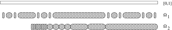
Figure 2. The first four distinct lengths, with multiplicities, of the Cantor String $\Omega_{1}$ and the fractal string $\Omega_{2}$.

Example 1.8 (A String with the Lengths of the Cantor String).

Let $\Omega_{2}$ be the fractal string that has the the same lengths as the Cantor String, but with the lengths arranged in non-increasing order from right to left. (See Figure 2.) This fractal string has the same geometric zeta function as the Cantor String, and thus the same Minkowski dimension, $\log_{3}2$; however, the Hausdorff dimension of the boundary of $\Omega_{2}$ is zero, whereas that of $\Omega_{1}$ is $\log_{3}2$ (by the self-similarity of the Cantor Set, see [8]). This follows immediately from the fact that the boundary is a set of countably many points. The multifractal zeta functions defined in Section 3 below will illustrate this difference and hence allow us to distinguish between the fractal strings $\Omega_{1}$ and $\Omega_{2}$.

The following key result, which can be found in [26, 29], uses the complex dimensions of a fractal string in a formula for the volume of the inner $\varepsilon$-neighborhoods of a fractal string.

Theorem 1.9.

Under mild hypotheses, the volume of the one-sided tubular neighborhood of radius $\varepsilon$ of the boundary of a fractal string $\Omega$ (with lengths $\mathcal{L}$) is given by the following explicit formula with error term:

$$V(\varepsilon)=\sum_{\omega\in\mathcal{D}_{\mathcal{L}}(W)\cup\{0\}}\textnormal{res}\left(\frac{\zeta_{\mathcal{L}}(s)(2\varepsilon)^{1-s}}{s(1-s)};\omega\right)+\mathcal{R}(\varepsilon),$$

where the error term can be estimated by $\mathcal{R}(\varepsilon)=\mathcal{O}(\varepsilon^{1-\sup r})$ as $\varepsilon\rightarrow 0^{+}.$

Remark 1.10.

In particular, in Theorem 1.9, if all the poles of $\zeta_{\mathcal{L}}$ are simple and $0\notin\mathcal{D}_{\mathcal{L}}(W),$ then

$$V(\varepsilon)=\sum_{\omega\in\mathcal{D}_{\mathcal{L}}(W)}\frac{2^{1-\omega}}{\omega(1-\omega)}\textnormal{res}(\zeta_{\mathcal{L}},\omega)\varepsilon^{1-\omega}+\mathcal{R}(\varepsilon).$$

Remark 1.11.

If $\mathcal{L}$ is a self-similar string (e.g., if its boundary is a self-similar subset of $\mathbb{R}$), then the conclusion of Theorem 1.9 holds with $\mathcal{R}(\varepsilon)\equiv 0.$ This is the case, in particular, for the Cantor String $\Omega_{1}$ and for $\Omega_{2}$ discussed in Examples 1.7 and 1.8.

2. Multifractal Analysis

Multifractal analysis is the study of measures which can be described as mass distributions whose concentrations of mass vary widely. In this section and throughout this text, we restrict our view to measures on the unit interval $[0,1]$. Example 2.1 below briefly discusses the construction of a multifractal measure on the Cantor set, with Figure 3 providing a few steps of the construction and the resulting multifractal spectrum, as found in Chapter 17 of [8].

Figure 3. (a) Construction of the binomial measure $\beta$. (b) The multifractal spectrum $f(\alpha)$ of the measure $\beta$.

Example 2.1 (A multifractal measure on the Cantor set).

A simple example of a multifractal measure is the binomial measure $\beta$ constructed on the classical Cantor set. To construct $\beta$, a mass distribution is added to the construction of the Cantor set which consists of a countable intersection of a nonincreasing sequence of closed intervals whose lengths tend to zero. Specifically, in addition to removing open middle thirds, weight is added at each stage. On the remaining closed intervals of each stage of the construction, place $1/3$ of the weight on the left interval and $2/3$ on the right, ad infinitum (see Figure 3). The measure found in the limit, denoted $\beta$, is a multifractal measure.

A notion which is key to the development of the multifractal zeta functions and is part of Example 2.1 is regularity. Regularity connects the size of a set with its mass. Specifically, let $\textbf{X}([0,1])$ denote the space of closed subintervals of $[0,1]$. The following definition can be found in [38] and is motivated by the large deviation spectrum and one of the continuous large deviation spectra in that paper.

Definition 2.2.

The regularity $A(U)$ of a Borel measure $\mu$ on $U\in\textnormal{{X}([0,1])}$ is

$$A(U)=\frac{\log\mu(U)}{\log{|U|}},$$

where $|\cdot|=\lambda(\cdot)$ is the Lebesgue measure on $\mathbb{R}$.

Regularity $A(U)$ is also known as the coarse Hölder exponent $\alpha$ which satisfies

$$|U|^{\alpha}=\mu(U).$$

We will consider regularity values $\alpha$ in the extended real numbers $[-\infty,\infty]$, where

$$\alpha=\infty=A(U)\Leftrightarrow\mu(U)=0\textnormal{ and }|U|>0,$$

and

$$\alpha=-\infty=A(U)\Leftrightarrow\mu(U)=\infty\textnormal{ and }|U|>0.$$

The original motivation for using the regularity values was to develop a family of zeta functions which would be parameterized by these values and would, in turn, generate a family of complex dimensions such as those from Section 1, but now indexed by the regularity exponent $\alpha\in[-\infty,\infty]$. A new kind of multifractal spectrum was to then be developed where the function values $f(\alpha)$ would be the real-valued dimensions (of some sort) corresponding to the regularity values $\alpha$. However, the multifractal zeta functions defined and discussed in the following sections are quite complicated and their application to examples such as Example 2.1 has yet to be thoroughly examined. Our view is restricted to measures that can be characterized as a collection of point-masses on the boundary of a fractal string. The results, therefore, are not rich enough to generate a full spectrum of dimension for the measures we consider. Nevertheless, multifractal zeta functions do regenerate the classical geometric zeta functions and reveal new topological zeta functions for fractal strings when examined via our restricted collection of measures. Analysis of multinomial measures using other families of zeta functions, whose definitions were motivated in part by those defined in the next section, has been done in [31, 32, 35, 47]. For other approaches to multifractal analysis, consider [1, 3, 4, 6, 7, 8, 12, 13, 14, 15, 16, 30, 31, 32, 33, 34, 36, 37, 39, 40, 41, 42, 43, 44, 45].

3. Multifractal Zeta Functions

In order to define multifractal zeta functions, we must understand the behavior of the measures with respect to their regularity values in significant detail. As such, more tools are provided below before the definition is given.

Let the collection of closed intervals with length $\eta\in(0,1)$ and regularity $\alpha$ be denoted by $\mathcal{R}_{\eta}(\alpha)$. Namely,

$$\mathcal{R}_{\eta}(\alpha)=\{U\in\textbf{X}([0,1])\hskip 5.69054pt|\hskip 5.69054pt|U|=\eta\textnormal{ and }A(U)=\alpha\}.$$

Consider the union of the sets in $\mathcal{R}_{\eta}(\alpha)$,

$$\bigcup_{\mathcal{R}_{\eta}(\alpha)}U:=\bigcup_{U\in\mathcal{R}_{\eta}(\alpha)}U.$$

Given $\alpha\in[-\infty,\infty]$ and $\eta\in(0,1)$, let

$$R^{\eta}(\alpha)=\bigcup_{\mathcal{R}_{\eta}(\alpha)}U.$$

For a scale $\eta>0$, $R^{\eta}(\alpha)$ is a disjoint union of a finite number of intervals, each of which may be open, closed or neither and are of length at least $\eta$ when $\mathcal{R}_{\eta}(\alpha)$ is non-empty. We will consider only discrete sequences of scales $\mathcal{N}=\{\eta_{n}\}_{n=1}^{\infty}$, with $\eta_{n}>0$ for all $n\geq 1$ and the sequence strictly decreasing to zero. So for $n\in\mathbb{N}$, let

$$R^{\eta_{n}}(\alpha)=R^{n}(\alpha).$$

We have

$$R^{n}(\alpha)=\bigcup_{p=1}^{r_{n}(\alpha)}R^{n}_{p}(\alpha),$$

where $r_{n}(\alpha)$ is the number of connected components $R^{n}_{p}(\alpha)$ of $R^{n}(\alpha)$. We denote the left and right endpoints of each interval $R^{n}_{p}(\alpha)$ by $a_{R}^{n}(\alpha,p)$ and $b_{R}^{n}(\alpha,p),$ respectively.

Given a sequence of positive real numbers $\mathcal{N}=\{\eta_{n}\}_{n=1}^{\infty}$ that tend to zero and a Borel measure $\mu$ on [0,1], we wish to examine the way $\mu$ changes with respect to a fixed regularity $\alpha$ between stages $n-1$ and $n$. Thus we consider the symmetric difference ($\ominus$) between $R^{n-1}(\alpha)$ and $R^{n}(\alpha)$. Let $J^{1}(\alpha)=R^{1}(\alpha),$ and for $n\geq 2$, let

$$J^{n}(\alpha)=R^{n-1}(\alpha)\ominus R^{n}(\alpha).$$

For all $n\in\mathbb{N}$, $J^{n}(\alpha)$ is also a disjoint union of intervals $J^{n}_{p}(\alpha)$, each of which may be open, closed, or neither. We have

$$J^{n}(\alpha)=\bigcup_{p=1}^{j_{n}(\alpha)}J^{n}_{p}(\alpha),$$

where $j_{n}(\alpha)$ is the number of connected components $J^{n}_{p}(\alpha)$ of $J^{n}(\alpha)$. The left and right endpoints of each interval $J^{n}_{p}(\alpha)$ are denoted by $a_{J}^{n}(\alpha,p)$ and $b_{J}^{n}(\alpha,p),$ respectively.

For a given regularity $\alpha\in[-\infty,\infty]$ and a measure $\mu$, the sequence $\mathcal{N}$ determines another sequence of lengths corresponding to the lengths of the connected components of the $J^{n}(\alpha)$. That is, the $J^{n}(\alpha)$ describe the way $\mu$ behaves between scales $\eta_{n-1}$ and $\eta_{n}$ with respect to $\alpha$. However, there is some redundancy with this set-up. Indeed, a particular regularity value may occur at all scales below a certain fixed scale in the same location. The desire to eliminate this redundancy will be clarified with some examples below. The next step is introduced to carry out this elimination.

Let $K^{1}(\alpha)=J^{1}(\alpha)=R^{1}(\alpha)$. For $n\geq 2$, let $K^{n}(\alpha)$ be the union of the subcollection of intervals in $J^{n}(\alpha)$ comprised of the intervals that have left and right endpoints distinct from, respectively, the left and right endpoints of the intervals in $R^{n-1}(\alpha)$. We have

$$K^{n}(\alpha)=\bigcup_{p=1}^{k_{n}(\alpha)}K^{n}_{p}(\alpha)\subset J^{n}(\alpha),$$

where $k_{n}(\alpha)$ is the number of connected components $K^{n}_{p}(\alpha)$ of $K^{n}(\alpha)$. That is, the $K^{n}_{p}(\alpha)$ are the $J^{n}_{p}(\alpha)$ such that $a^{n}_{J}(\alpha,p_{1})\neq a^{n-1}_{R}(\alpha,p_{2})$ and $b^{n}_{J}(\alpha,p_{1})\neq b^{n-1}_{R}(\alpha,p_{2})$ for all $p_{1}\in\{1,...,j_{n}(\alpha)\}$ and $p_{2}\in\{1,...,r_{n}(\alpha)\}.$ Collecting the lengths of the intervals $K^{n}_{p}(\alpha)$ allows one to define a generalization of the geometric zeta function of a fractal string by considering a family of geometric zeta functions parameterized by the regularity values of the measure $\mu$.

Definition 3.1.

The multifractal zeta function of a measure $\mu$, sequence $\mathcal{N}$ and with associated regularity value $\alpha$ $\in[-\infty,\infty]$ is

$$\zeta^{\mu}_{\mathcal{N}}(\alpha,s)=\sum_{n=1}^{\infty}\sum_{p=1}^{k_{n}(\alpha)}|K^{n}_{p}(\alpha)|^{s},$$

for Re$(s)$ large enough.

If we assume that, as a function of $s\in\mathbb{C}$, $\zeta^{\mu}_{\mathcal{N}}(\alpha,s)$ admits a meromorphic continuation to an open neighborhood of a window $W$, then we may also consider the poles of these zeta functions, as in the case of the complex dimensions of a fractal string (see Section 1).

Definition 3.2.

For a measure $\mu$, sequence $\mathcal{N}$ which tends to zero and regularity value $\alpha$, the set of complex dimensions with parameter $\alpha$ is given by

$$\mathcal{D}^{\mu}_{\mathcal{N}}(\alpha,W)=\{\omega\in W\hskip 5.69054pt|\hskip 5.69054pt\zeta^{\mu}_{\mathcal{N}}(\alpha,s)\textnormal{ has a pole at }\omega\}.$$

When $W=\mathbb{C}$, we simply write $\mathcal{D}^{\mu}_{\mathcal{N}}(\alpha)$.

The following sections consider two specific regularity values. In Section 4, the value $\infty$ generates the geometric zeta function for the complement of the support of the measure in question. In Section 5, the value $-\infty$ generates the topological zeta function which detects some topological properties of fractal strings that are ignored by the geometric zeta functions when certain measures are considered.

4. Regularity Value $\infty$ and Geometric Zeta Functions

The geometric zeta function is recovered as a special case of multifractal zeta functions. Specifically, regularity value $\alpha=\infty$ yields the geometric zeta function of the complement of the support of a given positive Borel measure $\mu$ on $[0,1]$.

To see how this is done, let $E^{c}$ denote the complement of $E$ in $[0,1]$ and consider the fractal string $(supp(\mu))^{c}=\Omega_{\mu}$ whose lengths $\mathcal{L}_{\mu}$ are those of the disjoint intervals $(a_{j},b_{j})$ where $\Omega_{\mu}=\cup_{j=1}^{\infty}(a_{j},b_{j})$. Let $\{\ell_{j}\}_{j=1}^{\infty}$ be the lengths of $\mathcal{L}_{\mu}$. Thus,

$$\{\ell_{j}\}_{j=1}^{\infty}=|(a_{j},b_{j})|=b_{j}-a_{j}.$$

Further, let $\{l_{n}\}_{n=1}^{\infty}$ be the distinct lengths of $\mathcal{L}_{\mu}$ with multiplicities $\{m_{n}\}_{n=1}^{\infty}$.

Figure 4. Key for the construction of the lengths used to define the multifractal zeta functions.

The following technical lemma is used in the proof of the theorem below which shows the recovery of the geometric zeta function as the multifractal zeta function with regularity $\infty$. See Figures 4 and 5 for an illustration of the construction of a multifractal zeta function with regularity $\infty$ for a measure which is supported on the Cantor set.

Lemma 4.1.

Suppose $\{x\}=supp(\mu)\cap U$ for some $U\in\textnormal{{X}}([0,1])$. Then

$$A(U)=\infty\Leftrightarrow\mu(\{x\})=0.$$

Proof.

$\mu(\{x\})\neq 0\Leftrightarrow\mu(U)>|U|\Leftrightarrow A(U)\neq\infty.$ ∎

The lemma helps deal with the subtle interactions between the closed intervals $U$ of size $\eta_{n}$ and the support of $\mu$, essentially allowing us to prove a single case of the following theorem without loss of generality.

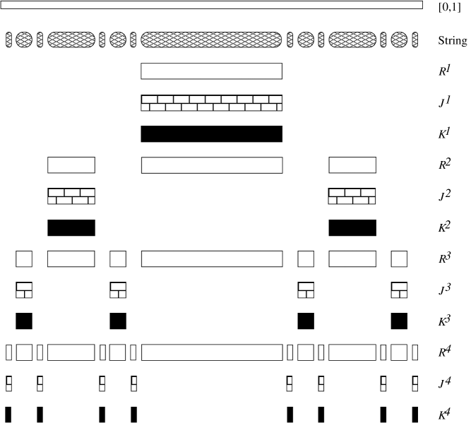
Figure 5. Construction of the multifractal zeta function $\zeta^{\mu}_{\mathcal{N}}(\infty,s)$ as in the proof of Theorem 4.2.

Theorem 4.2.

The multifractal zeta function of a positive Borel measure $\mu$, any sequence $\mathcal{N}$ such that $\eta_{n}\searrow 0$ and regularity $\alpha=\infty$ is the geometric zeta function of $(supp(\mu))^{c}$. That is,

$$\zeta^{\mu}_{\mathcal{N}}(\infty,s)=\zeta_{\mathcal{L}_{\mu}}(s).$$

Proof.

Recall the notation introduced at the beginning of Section 3. For all $n\in\mathbb{N}$,

$$U\in\mathcal{R}_{\eta_{n}}(\infty)\Leftrightarrow A(U)=\frac{\log(\mu(U))}{\log|U|}=\infty\hskip 5.69054pt\textnormal{and}\hskip 5.69054pt|U|=\eta_{n}.$$

Therefore, $\forall n\in\mathbb{N},U\in\mathcal{R}_{\eta_{n}}(\infty)$ only if $\mu(U)=0$.

The sets $\mathcal{R}_{\eta_{n}}(\infty)$ depend further upon whether any of the endpoints of the intervals $I_{j}=(a_{j},b_{j})$ which comprise $\Omega_{\mu}=(supp(\mu))^{c}$ contain mass as singletons. If $\mu(\{a_{j}\})\neq 0$ and $\mu(\{b_{j}\})\neq 0$ for all $j\in\mathbb{N}$, then $R^{n}(\infty)=\bigcup_{\ell_{j}>\eta_{n}}I_{j}\subset\Omega_{\mu}.$

Lemma 4.1 implies that, without loss of generality, we need only consider the case where every endpoint contains mass. Suppose $\mu(\{a_{j}\})\neq 0$ and $\mu(\{b_{j}\})\neq 0$ for all $j\in\mathbb{N}$. Then $R^{n}(\infty)=\bigcup_{\ell_{j}>\eta_{n}}I_{j}$ implies that, for $n\geq 2$,

$$J^{n}(\infty) = \Bigg{(}\bigcup_{\ell_{j}>\eta_{n-1}}I_{j}\Bigg{)}\ominus\Bigg{(}\bigcup_{\ell_{j}>\eta_{n}}I_{j}\Bigg{)}$$

$$= \Bigg{(}\bigcup_{\ell_{j}>\eta_{n}}I_{j}\Bigg{)}\setminus\Bigg{(}\bigcup_{\ell_{j}>\eta_{n-1}}I_{j}\Bigg{)}$$

$$= \bigcup_{\eta_{n-1}\geq\ell_{j}>\eta_{n}}I_{j}.$$

Since $R^{n-1}(\infty)\subset R^{n}(\infty)$ for all $n\geq 2$, the intervals $J^{n}(\infty)$ have no redundant lengths. That is, $a_{J}^{n}(\infty,p_{1})\neq a_{R}^{n-1}(\infty,p_{2})$ and $b_{J}^{n}(\infty,p_{1})\neq b_{R}^{n-1}(\infty,p_{2})$ for all $n\geq 2$ and $p_{1},p_{2}\in\{1,...,j_{n}(\infty)\}$. This implies

$$K^{n}(\infty)=J^{n}(\infty)=\bigcup_{\eta_{n-1}\geq\ell_{j}>\eta_{n}}I_{j}.$$

Furthermore,

$$|K^{n}(\infty)|=\sum_{p=1}^{k_{n}(\infty)}|K^{n}_{p}(\infty)|=\sum\ell_{j},$$

where the last sum is taken over all $j$ such that $\eta_{n-1}\geq\ell_{j}>\eta_{n}$. Since $\eta_{n}\searrow 0$, each length $\ell_{j}$ is eventually picked up. Therefore,

$$\zeta^{\mu}_{\mathcal{N}}(\infty,s) = \sum_{n=1}^{\infty}\sum_{p=1}^{k_{n}(\infty)}|K^{n}_{p}(\infty)|^{s}=\sum_{n=1}^{\infty}\sum\ell_{j}^{s}$$

$$= \sum_{n=1}^{\infty}m_{n}l_{n}^{s}=\zeta_{\mathcal{L}_{\mu}}(s).$$

∎

Corollary 4.3.

Under the assumptions of Theorem 4.2, the complex dimensions of the fractal string $\Omega_{\mu}=(supp(\mu))^{c}$ coincide with the poles of the multifractal zeta function $\zeta^{\mu}_{\mathcal{N}}(\infty,s)$. That is,

$$\mathcal{D}_{\mathcal{N}}^{\mu}(\infty,W)=\mathcal{D}_{\mathcal{L_{\mu}}}(W)$$

for every window $W$.

The key in Figure 4 will be used for the examples that analyze the fractal strings below. Figure 5 shows the first four steps in the construction of a multifractal zeta function with regularity $\infty$ for a measure supported on the Cantor set.

Remark 4.4.

Assume $supp(\mu)$ has empty interior, as is the case, for example, if $supp(\mu)$ is a Cantor set. It then follows from Theorem 4.2 that $D_{\mathcal{L}_{\mu}}$, the abscissa of convergence of $\zeta^{\mu}_{\mathcal{N}}(\infty,s)$, is the Minkowski dimension of $\partial\Omega_{\mu}=supp(\mu).$ Note that as long as the sequence decreases to zero, the choice of sequence of scales $\mathcal{N}$ does not affect the result of Theorem 4.2. This is not the case, however, for other regularity values.

The following section describes a measure which is designed to illuminate properties of a given fractal string and justifies calling the multifractal zeta function with regularity $-\infty$ the topological zeta function.

5. Regularity Value $-\infty$ and Topological Zeta Functions

The remainder of this paper deals with fractal strings that have a countably infinite number of lengths. If there are only a finite number of lengths, it can be easily verified that all of the corresponding zeta functions are entire because the measures taken into consideration are then comprised of a finite number of unit point-masses. Thus we consider certain measures that have infinitely many unit point-masses. More specifically, in this section we consider a fractal string $\Omega$ to be a subset of $[0,1]$ comprised of countably many open intervals $(a_{j},b_{j})$ such that $|\Omega|=1$ and $\partial\Omega=[0,1]\backslash\Omega$ (or equivalently, $\Omega^{c}=[0,1]\backslash\Omega$ has empty interior). We also associate to $\Omega=\cup_{j=1}^{\infty}(a_{j},b_{j})$ its sequence of lengths $\mathcal{L}$. For such $\Omega$, the endpoints of the intervals $(a_{j},b_{j})$ are dense in $\partial\Omega$. Indeed, if there were a point in $\partial\Omega$ away from any endpoint, then it would be away from $\Omega$ itself, meaning it would not be in $\partial\Omega$. This allows us to define, in a natural way, measures with a countable number of point-masses contained in the boundary of $\Omega$. Let

$$\mu_{\Omega}:=\sum_{j=1}^{\infty}(\delta_{a_{j}}+\delta_{b_{j}}),$$

where, as above, the $(a_{j},b_{j})$ are the open intervals whose disjoint union is $\Omega$.

Let us determine the nontrivial regularity values $\alpha$. For $\alpha=\infty$, $\mathcal{R}_{\eta_{n}}(\infty)$ is the collection of closed intervals of length $\eta_{n}$ which contain no point-masses. For $\alpha=-\infty$, $\mathcal{R}_{\eta_{n}}(-\infty)$ is the collection of closed intervals of length $\eta_{n}$ which contain infinitely many point-masses. In other words, $\mathcal{R}_{\eta_{n}}(-\infty)$ is the collection of closed intervals of length $\eta_{n}$ that contain a neighborhood of an accumulation point of the endpoints of $\Omega$. This connection motivates the following definition.

Definition 5.1.

Let $\Omega$ be a fractal string and consider the corresponding measure $\mu_{\Omega}=\sum_{j=1}^{\infty}(\delta_{a_{j}}+\delta_{b_{j}})$. The topological zeta function of $\Omega$ with respect to the sequence $\mathcal{N}$ is $\zeta^{\mu_{\Omega}}_{\mathcal{N}}(-\infty,s)$, the multifractal zeta function of $\mu_{\Omega}$ with respect to $\mathcal{N}$ and regularity $-\infty$.

When the open set $\Omega$ has a perfect boundary, there is a relatively simple breakdown of all the possible multifractal zeta functions for the measure $\mu_{\Omega}$. Recall that a set is perfect if it is equal to its set of accumulation points. For example, the Cantor set is perfect; more generally, all self-similar sets are perfect (see, e.g., [8]). The boundary of a fractal string is closed; hence, it is perfect if and only if it does not have any isolated point. The simplicity of the breakdown is due to the fact that every point-mass is a limit point of other point-masses. Consequently, the only parameters $\alpha$ that do not yield identically zero multifractal zeta functions are $\infty$, $-\infty$ and those which correspond to each length of $\mathcal{N}$ and one or two point-masses.

Theorem 5.2.

For a fractal string $\Omega=\bigcup_{j=1}^{\infty}(a_{j},b_{j})$ with sequence of lengths $\mathcal{L}$ and perfect boundary, consider $\mu_{\Omega}=\sum_{j=1}^{\infty}(\delta_{a_{j}}+\delta_{b_{j}}).$ Suppose that $\mathcal{N}$ is a sequence such that $l_{n}>\eta_{n}\geq l_{n+1}$ and $l_{n}>2\eta_{n},$ for all $n\in\mathbb{N}.$ Then

$$\zeta^{\mu_{\Omega}}_{\mathcal{N}}(\infty,s)=\zeta_{\mathcal{L}}(s)$$

and

$$\zeta^{\mu_{\Omega}}_{\mathcal{N}}(-\infty,s)=h(s)+\sum_{n=2}^{\infty}m_{n}(l_{n}-2\eta_{n})^{s},$$

where $h(s)$ is the entire function given by $h(s)=\sum_{p=1}^{k_{1}(-\infty)}|K^{1}_{p}(-\infty)|^{s}.$ Moreover, for every real number $\alpha$ (i.e., for $\alpha\neq\infty,-\infty$), $\zeta^{\mu_{\Omega}}_{\mathcal{N}}(\alpha,s)$ is entire.

Proof.

$\zeta^{\mu_{\Omega}}_{\mathcal{N}}(\infty,s)=\zeta_{\mathcal{L}}(s)$ holds by Theorem 4.2. Since $l_{n}>2\eta_{n}$, we have

$$R^{n}(-\infty)=\left(\bigcup_{\ell_{j}>\eta_{n}}[a_{j}+\eta_{n},b_{j}-\eta_{n}]\right)^{c}.$$

For $n\geq 2$, $J^{n}(-\infty)$ is made up of $m_{n}$ intervals of length $l_{n}-2\eta_{n}$ and $2\sum_{p=1}^{n-1}m_{p}$ intervals of length $\eta_{n-1}-\eta_{n}$. That is, at each stage $n\geq 2$, we pick up two $\eta_{n-1}-\eta_{n}$ terms for each $\ell_{j}\geq l_{n-1}$ from the previous stage and one $l_{n}-2\eta_{n}$ term for each $\ell_{j}=l_{n}$. By construction, the sets $K^{n}(-\infty)$ do not include the redundant $\eta_{n-1}-\eta_{n}$ terms. Therefore,

$$\zeta^{\mu_{\Omega}}_{\mathcal{N}}(-\infty,s)=\sum_{p=1}^{k_{1}(-\infty)}|K^{1}_{p}(-\infty)|^{s}+\sum_{n=2}^{\infty}m_{n}(l_{n}-2\eta_{n})^{s}.$$

To prove the last statement in the theorem, note that any given interval $U\in$ X([0,1]) may contain 0, 1, 2 or infinitely many endpoints, each of which has a unit point-mass. Indeed, if $U$ contained an open neighborhood of a point in a perfect set it would necessarily contain an infinite number of points. If an interval $U$ contains 1 or 2 endpoints, the corresponding regularity would appear only at the stage corresponding to the scale $\eta$ which generated $U$ and perhaps one more stage. Thus, there are at most two stages contributing lengths to the multifractal zeta function with the same regularity. It follows that the multifractal zeta function has finitely many terms of the form $\ell^{s}$ where $\ell\in[0,1]$, and hence is entire.

∎

Remark 5.3.

If one were to envision a kind of multifractal spectrum for the measures $\mu_{\Omega}$ which satisfy the conditions of Theorem 5.2 in terms of a function $f(\alpha)$ whose output values are abscissae of convergence of multifractal zeta functions, the spectrum would be very simple: only regularity values $\alpha=\pm\infty$ could generate positive values for $f(\alpha)$. If the weights of the point-masses for some $\mu_{\Omega}$ were not all the not same, as in the measure $\nu$ from [38], other values of $\alpha$ may be shown to yield positive $f(\alpha)$ and thus $\nu$ may have a more interesting multifractal spectrum. See [47] for further elaboration on this perspective.

For certain fractal strings with perfect boundaries and a naturally chosen sequence, Theorem 5.2 has the following corollary.

Corollary 5.4.

Assume that $\Omega$ is a fractal string with perfect boundary, total length 1, and distinct lengths $\mathcal{L}$ given by $l_{n}=ca^{-n}$ with multiplicities $m_{n}$ for some $a>2$ and $c>0$. Further, assume that $\mathcal{N}$ is a sequence of scales where $\eta_{n}=l_{n+1}=ca^{-n-1}$, then

$$\zeta^{\mu_{\Omega}}_{\mathcal{N}}(-\infty,s)=f_{0}(s)+f_{1}(s)\zeta_{\mathcal{L}}(s),$$

where $f_{0}(s)$ and $f_{1}(s)$ are entire.

Proof.

By Theorem 5.2,

$$\zeta^{\mu_{\Omega}}_{\mathcal{N}}(-\infty,s) = h(s)+\sum_{n=2}^{\infty}m_{n}(l_{n}-2l_{n+1})^{s}$$

$$= h(s)+c^{s}\left(\frac{a-2}{a}\right)^{s}\left(\zeta_{\mathcal{L}}(s)-m_{1}a^{-s}\right).$$

Therefore, the result holds with

$$f_{0}(s):=h(s)-m_{1}c^{s}\left(\frac{a-2}{a^{2}}\right)^{s}\hskip 19.91692pt\textnormal{and}\hskip 19.91692ptf_{1}(s):=c^{s}\left(\frac{a-2}{a}\right)^{s}.$$

∎

Remark 5.5.

Corollary 5.4 clearly shows that, in general, the topological zeta functions of the form $\zeta^{\mu_{\Omega}}_{\mathcal{N}}(-\infty,s)$ may have poles. Indeed, since $f_{1}(s)$ has no zeros, we have that $\mathcal{D}^{\mu}_{\mathcal{N}}(-\infty,W)=\mathcal{D}_{\mathcal{L}}(W)$ for any window $W$.

Remark 5.6.

There are a few key differences between the result of Theorem 4.2 and the results in this section. For regularity $\alpha=\infty$, the form of the multifractal zeta function is independent of the choice of the sequence of scales $\mathcal{N}$ and the topological configuration of the fractal string in question. For other regularity values, however, this is not the case. In particular, regularity value $\alpha=-\infty$ sheds some light on the topological properties of the fractal string in a way that depends on $\mathcal{N}$. This dependence on the choice of scales is a very common feature in multifractal analysis.)

We now define a special sequence that describes the collection of accumulation points of the boundary of a fractal string $\Omega$.

Definition 5.7.

The sequence of effective lengths of a fractal string $\Omega$ with respect to the sequence $\mathcal{N}$ is

$$\mathcal{K}^{\mu_{\Omega}}_{\mathcal{N}}(-\infty):=\{|K^{n}_{p}(-\infty)|\hskip 5.69054pt|\hskip 5.69054ptn\in\mathbb{N},\hskip 5.69054ptp\in\{1,...,k_{n}(-\infty)\}\},$$

where $\mu_{\Omega}=\sum_{j=1}^{\infty}(\delta_{a_{j}}+\delta_{b_{j}}).$

This definition is motivated by a key property of the Hausdorff dimension $dim_{H}$: it is countably stable, that is,

$$dim_{H}(\cup_{n=1}^{\infty}A_{n})=\sup_{n\geq 1}dim_{H}(A_{n}).$$

(For this and other properties of $dim_{H}$, see [8].) Consequently, countable sets have Hausdorff dimension zero. As such, countable collections of isolated points do not contribute to the Hausdorff dimension of a given set. Regularity $-\infty$ picks up closed intervals of all sizes $\eta_{n}\in\mathcal{N}$ that contain an open neighborhood of an accumulation point of the boundary of the fractal string $\Omega$. The effective sequence (and hence its multifractal zeta function) describes the gaps between these accumulation points as detected at all scales $\eta_{n}\in\mathcal{N}$, which we now define.

The distinct gap lengths are the distinct sums $g_{k}:=\sum\ell_{j}$ where $k\in\mathbb{N}$ and the sums are taken over all $j$’s such that the disjoint subintervals $I_{j}=(a_{j},b_{j})$ of $\Omega$ are adjacent and have rightmost and/or leftmost endpoints (or limits thereof) which are 0, 1 or accumulation points of $\partial\Omega$. The effective lengths have the following description: For the scale $\eta_{1}$, $K^{1}(-\infty)$ is the union of the collection of connected components of $R^{1}(-\infty)$. For $\eta_{n}$ such that $n\geq 2$, $|K^{n}_{p}(-\infty)|=g_{k}-\eta_{n}$ if $\eta_{n}$ is the scale that first detects the gap $g_{k}$, that is, if $\eta_{n}$ is the unique first scale $\eta_{k}^{E}$ such that $2\eta_{n-1}>g_{k}\geq 2\eta_{n}.$

Under appropriate re-indexing, the effective lengths with multiplicities $m_{E,k}$ (other than $K^{1}(-\infty)$) are $\{l_{E,k}\}_{k\geq 2}$, given by $l_{E,k}:=g_{k}-2\eta_{k}^{E},$ where the gaps $g_{k}$ are those such that $2\eta_{1}>g_{k}$ and the $\eta_{k}^{E}\in\mathcal{N}_{E}\subset\mathcal{N}$ are the effective scales with respect to $\mathcal{N}$ that detect these gaps. The result is summarized in the next theorem, which gives a formula for the multifractal zeta function of the measure $\mu_{\Omega}$ with sequence of scales $\mathcal{N}$ at regularity $-\infty$. The second formula in Theorem 5.2 above can be viewed as a corollary to this theorem. Note that the assumption of a perfect boundary is not needed in the following result.

Theorem 5.8.

For a fractal string $\Omega$ with sequence of lengths $\mathcal{L}$ and for a sequence of scales $\mathcal{N}$ such that $\eta_{n}\searrow 0$, the topological zeta function is given by

$$\zeta^{\mu_{\Omega}}_{\mathcal{N}}(-\infty,s) = \sum_{p=1}^{k_{1}(-\infty)}|K^{1}_{p}(-\infty)|^{s}+\sum_{k=1}^{\infty}m_{E,k}l_{E,k}^{s},$$

for Re$(s)$ large enough.

The next section investigates the application of the results of Sections 4 and 5 to the Cantor String, as defined in Section 1, and the variants thereof.

6. Variants of the Cantor String

Let $\mathcal{L}$ be the sequence of lengths in the complement of the Cantor set, which is also known as the Cantor String $\Omega_{1}$. (See Example 1.7 and Figure 2.) Then $l_{n}=3^{-n}$ and $m_{n}=2^{n-1}$ for all $n$. We will discuss three examples of fractal strings involving this sequence of lengths, but for now consider the following one.

Let $\Omega_{2}$ be the open subset of $[0,1]$ whose lengths are also $\mathcal{L}$ but arranged in non-increasing order from right to left, as in Example 1.8. That is, the only accumulation point of $\partial\Omega_{2}$ is $0$ (see Figures 4, 6 and 7). In each figure, portions of the approximation of the string that appear adjacent are actually separated by a single point in the support of the measure. Gaps between the different portions and the points 0 and 1 contain the smaller portions of the string, isolated endpoints and accumulation points of endpoints.

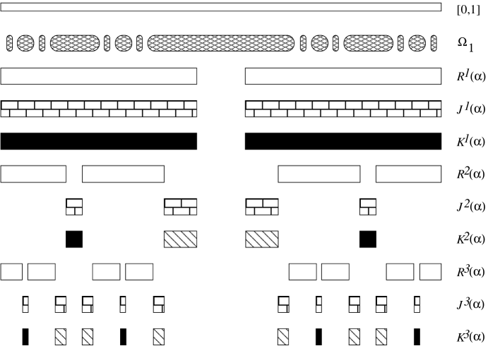
Figure 6. The first three stages in the construction of the topological zeta function of $\Omega_{1}$, $\zeta^{\mu_{1}}_{\mathcal{N}}(-\infty,s),$ where $\mathcal{N}$ is the set of distinct lengths of the Cantor String beginning with 1/9.

Consider the following measures which have singularities on a portion of the boundary of $\Omega_{1}$ and $\Omega_{2}$, respectively: $\mu_{q}=\mu_{\Omega_{q}}$, with $q=1$ or $2$, where $\mu_{\Omega_{q}}$ is defined as in Section 5. These measures have a unit point-mass at every endpoint of the intervals which comprise $\Omega_{1}$ and $\Omega_{2}$, respectively.

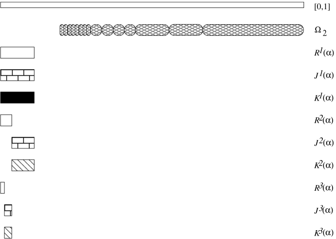
Figure 7. The first three stages in the construction of the topological zeta function of $\Omega_{2}$, $\zeta^{\mu_{2}}_{\mathcal{N}}(-\infty,s),$ where $\mathcal{N}$ is the set of distinct lengths of the Cantor String beginning with 1/9.

Let $\mathcal{N}$ be such that $l_{n}>\eta_{n}\geq l_{n+1}$ and $l_{n}>2\eta_{n}$. Such sequences exist for the Cantor String. For instance, $\forall n\in\mathbb{N}$, let $\eta_{n}=l_{n+1}=3^{-n-1}.$ Theorem 4.2 yields

$$\zeta^{\mu_{1}}_{\mathcal{N}}(\infty,s)=\zeta^{\mu_{2}}_{\mathcal{N}}(\infty,s)=\zeta_{CS}(s).$$

When $\alpha=-\infty$ the topological zeta functions for $\Omega_{1}$ and $\Omega_{2}$ are, respectively,

$$\zeta^{\mu_{1}}_{\mathcal{N}}(-\infty,s)=2(l_{1}+\eta_{1})^{s}+\sum_{n=2}^{\infty}2^{n-1}(l_{n}-2\eta_{n})^{s}$$

and

$$\zeta^{\mu_{2}}_{\mathcal{N}}(-\infty,s)=\eta_{1}^{s}.$$

In either case,

$$-\infty=A(U) = \frac{\sum_{a_{j},b_{j}\in U}1}{\log|U|}$$

if and only if

$$\#\{j\hskip 5.69054pt|\hskip 5.69054pta_{j}\in U\}+\#\{j\hskip 5.69054pt|\hskip 5.69054ptb_{j}\in U\}=\infty.$$

In the case of $\mu_{2}$, the only closed interval of length $\eta_{n}$ that contains infinitely many unit point-masses is $[0,\eta_{n}]$. So,

$$R^{n}(-\infty)=[0,\eta_{n}]$$

which means

$$J^{1}(-\infty)=K^{1}(-\infty)=[0,\eta_{1}]$$

and for $n\geq 2$,

$$J^{n}(-\infty)=(\eta_{n},\eta_{n-1}].$$

All of the terms from $J^{n}(-\infty)=(\eta_{n},\eta_{n-1}]$ are redundant. Therefore,

$$K^{n}(-\infty)=\emptyset$$

and

$$\zeta^{\mu_{2}}_{\mathcal{N}}(-\infty,s)=\eta_{1}^{s}.$$

The case of $\mu_{1}$ for regularity $\alpha=-\infty$ is more complicated and is a result of Theorem 5.2. This is due to the fact that every point-mass is a limit point of other point-masses. That is, the Cantor set is a perfect set, thus Corollary 5.4 applies when $\mathcal{N}$ is chosen so that $\eta_{n}=3^{-n-1}$ for all $n\in\mathbb{N}$.

Remark 6.1.

Clearly, for every $\mathcal{N}$ chosen as above in the discussion of $\mu_{2}$, $\mathcal{D}^{\mu_{2}}_{\mathcal{N}}(-\infty)$ is empty. In contrast, it follows from the above discussion that it is easy to find a sequence $\mathcal{N}$ such that $\mathcal{D}^{\mu_{1}}_{\mathcal{N}}(-\infty)$ is non-empty and even countably infinite.

Shortly we will consider another fractal string, $\Omega_{3}$, in addition to the Cantor String $\Omega_{1}$ and the string $\Omega_{2}$. All of these fractal strings have the same sequence of lengths. As such, these strings all have the same Minkowski dimension, namely $\log_{3}{2}$. However, their respective Hausdorff dimensions do not coincide, a fact that is detected by the topological zeta functions but the theory of fractal strings developed in [26, 29] does not describe. For a certain, natural choice of sequence of scales $\mathcal{N}$, the topological zeta functions of the fractal strings $\Omega_{q}$ (as above) have poles on a discrete line above and below the Hausdorff dimension of the boundaries of these fractal strings (see Figures 4 and 6–8). In [26, 29] it is shown that the complex dimensions of the fractal strings $\Omega_{q}$, for $q=1,2,3$ are

$$\mathcal{D}_{CS}=\left\{\log_{3}{2}+\frac{2i\pi m}{\log 3}\hskip 5.69054pt|\hskip 5.69054ptm\in\mathbb{Z}\right\}.$$

These are the poles of

$$\zeta^{\mu_{q}}_{\mathcal{N}}(\infty,s)=\zeta_{CS}(s)=\frac{3^{-s}}{1-2\cdot 3^{-s}}.$$

(See Section 1 above.) As noted earlier, the geometric zeta function of the Cantor String does not see any difference between the open sets $\Omega_{q}$, for $q=1,2,3$. However, the multifractal zeta functions of the measures $\mu_{q}$ with the same such $\mathcal{N}$ and regularity $\alpha=-\infty$ are quite different. For the remainder of this section, unless explicitly stated otherwise, we choose $\mathcal{N}=\{3^{-n-1}\}_{n=1}^{\infty}$.

We now consider more specifically the fractal string $\Omega_{3}$ mentioned above. This fractal string is comprised of a Cantor-like string and an isolated accumulation point at 1. The lengths comprising the Cantor-like string are constructed by connecting two intervals with consecutive lengths. The remaining lengths are arranged in non-increasing order from left to right, accumulating at 1. That is, for $n\geq 1$, the gap lengths are $3^{-2n+1}+3^{-2n}=4\cdot 3^{-2n}$ with multiplicities $2^{n-1}$ and therefore the effective lengths are $2\cdot 3^{-2n}$ with multiplicities $2^{n-1}$. (See Figure 8.)

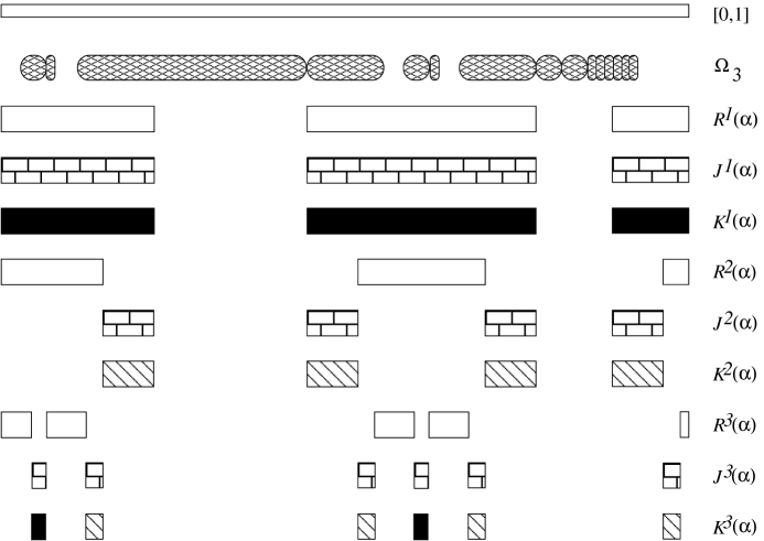
Figure 8. The first three stages in the construction of the topological zeta function of $\Omega_{3}$, $\zeta^{\mu_{3}}_{\mathcal{N}}(-\infty,s),$ where $\mathcal{N}$ is the set of distinct lengths of the Cantor String beginning with 1/9.

The Hausdorff dimension of the boundary of each fractal string $\Omega_{q}$ ($q=1,2,3$) is easily determined. For a set $F$, denote the Hausdorff dimension by $dim_{H}(F)$ and the Minkowski dimension by $dim_{M}(F)$. We have, for $q=1,2,3$:

$$dim_{H}(\partial\Omega_{1})=dim_{M}(\partial\Omega_{q}) = \log_{3}{2},$$

$$dim_{H}(\partial\Omega_{2}) = 0,$$

$$dim_{H}(\partial\Omega_{3}) = \log_{9}{2}.$$

The first line in the displayed equation above holds since the Minkowski dimension depends only on the lengths of the fractal strings and, furthermore, the Cantor set $\partial\Omega_{1}$ is a strictly self-similar set whose similarity transformations satisfy the open set condition, as defined, for example, in [8]. Thus, the Minkowski and Hausdorff dimensions coincide for $\partial\Omega_{1}$. The second equality holds because $\partial\Omega_{2}$ is a countable set. The third holds because $\partial\Omega_{3}$ is the disjoint union of a strictly self-similar set and a countable set, and Hausdorff dimension is (countably) stable. We justify further below.

Theorem 5.2, Corollary 5.4, and Theorem 5.8 will be used to generate the following closed forms of the zeta functions $\zeta^{\mu_{q}}_{\mathcal{N}}(-\infty,s).$

For the Cantor String $\Omega_{1}$ and the corresponding measure $\mu_{1}$, we have by Corollary 5.4,

$$\zeta^{\mu_{1}}_{\mathcal{N}}(-\infty,s) = 2\left(\frac{1}{3}+\frac{1}{9}\right)^{s}+\sum_{n=2}^{\infty}2^{n-1}\left(\frac{1}{3^{n}}-\frac{2}{3^{n+1}}\right)^{s}$$

$$= 2\left(\frac{4}{9}\right)^{s}+\frac{2}{27^{s}}\left(\frac{1}{1-2\cdot 3^{-s}}\right).$$

The poles of $\zeta^{\mu_{1}}_{\mathcal{N}}(-\infty,s)$ are the same as the poles of the geometric zeta function of the Cantor String. They are given by

$$\mathcal{D}^{\mu_{1}}_{\mathcal{N}}(-\infty)=\left\{\log_{3}{2}+\frac{2i\pi m}{\log 3}\hskip 5.69054pt|\hskip 5.69054ptm\in\mathbb{Z}\right\}=\mathcal{D}_{CS}.$$

Remark 6.2.

Note that the above computation of $\zeta^{\mu_{1}}_{\mathcal{N}}(-\infty,s)$ is justified, a priori, for Re$(s)>\log_{3}2.$ However, by analytic continuation, it clearly follows that $\zeta^{\mu_{1}}_{\mathcal{N}}(-\infty,s)$ has a meromorphic continuation to all of $\mathbb{C}$ and is given by the same resulting expression for every $s\in\mathbb{C}.$ Analogous comments apply to similar computations elsewhere in the paper.

Since $\partial\Omega_{2}$ has only one accumulation point, there is only one term in the corresponding topological zeta function for $\Omega_{2}$. We immediately have

$$\zeta^{\mu_{2}}_{\mathcal{N}}(-\infty,s)=\frac{1}{9^{s}},$$

which, of course, is entire and has no poles.

For $\Omega_{3}$, we have

$$\zeta^{\mu_{3}}_{\mathcal{N}}(-\infty,s) = h_{3}(s)+\sum_{n=2}^{\infty}m_{n}\left(l_{2n-1}+l_{2n}-2\eta_{2n-1}\right)^{s}$$

$$= h_{3}(s)+\left(\frac{2^{s+1}}{81^{s}}\right)\left(\frac{1}{1-2\cdot 9^{-s}}\right),$$

where $h_{3}(s)$ is entire. Therefore, the poles of $\zeta^{\mu_{3}}_{\mathcal{N}}(-\infty,s)$ are given by

$$\mathcal{D}^{\mu_{3}}_{\mathcal{N}}(-\infty)=\left\{\log_{9}{2}+\frac{2i\pi m}{\log 9}\hskip 5.69054pt|\hskip 5.69054ptm\in\mathbb{Z}\right\}.$$

Let us summarize the results of this section. We chose the sequence of scales $\mathcal{N}$ to be $\{3^{-n-1}\}_{n=1}^{\infty}$. For $q=1,2,3$, the multifractal zeta function of each measure $\mu_{q}$ with regularity $\alpha=\infty$ is equal to the geometric zeta function of the Cantor String, as follows from Theorem 4.2. Thus, obviously, the collections of poles $\mathcal{D}^{\mu_{q}}_{\mathcal{N}}(\infty)$ each coincide with the complex dimensions of the Cantor String.

For regularity $\alpha=-\infty$, the multifractal zeta functions are the topological zeta functions for the fractal strings $\Omega_{q}$. The respective sets of complex dimensions $\mathcal{D}_{\mathcal{N}}^{\mu_{q}}(-\infty)$ differ for each $q=1,2,3$. Specifically, $\mathcal{D}_{\mathcal{N}}^{\mu_{1}}(-\infty)$ is exactly the same set of poles as $\mathcal{D}_{\mathcal{N}}^{\mu_{1}}(\infty)$ (and $\mathcal{D}_{CS}$), corresponding to the fact that $\partial\Omega_{1}$ has equal Minkowski and Hausdorff dimensions. Furthermore, since $\zeta^{\mu_{2}}_{\mathcal{N}}(-\infty,s)$ is an entire function, $\mathcal{D}_{\mathcal{N}}^{\mu_{2}}(-\infty)$ is the empty set. Additionally, $\partial\Omega_{2}$ has Hausdorff dimension equal to zero. Finally, $\mathcal{D}_{\mathcal{N}}^{\mu_{3}}(-\infty)$ is a discrete line of poles above and below the Hausdorff dimension of $\partial\Omega_{3}$, which is $\log_{9}{2}$. In all of these cases, the multifractal zeta functions with regularity $-\infty$ and their corresponding poles depend heavily on the choice of sequence of scales $\mathcal{N}$.

This section further illustrates the dependence of the multifractal zeta function with regularity $\alpha=-\infty$ on the topological configuration of the fractal string in question as well as the choice of scales $\mathcal{N}$ used to examine the fractal string. As before, following Theorem 4.2, regularity $\alpha=\infty$ corresponds to a multifractal zeta function that depends only on the lengths of the fractal string in question.

7. Concluding Comments

The main object defined in this paper, the multifractal zeta function, was originally designed to provide a new approach to multifractal analysis of measures which exhibit fractal structure in a variety of ways. In the search for examples with which to work, the authors found that the multifractal zeta functions can be used to describe some aspects of fractal strings that extend the existing notions garnered from the theory of geometric zeta functions and complex dimensions of fractal strings developed in [26, 29].

Regularity value $\alpha=\infty$ has been shown to precisely recover the geometric zeta function of the complement in [0,1] of the support of a measure which is singular with respect to the Lebesgue measure. This recovery is independent of the topological configuration of the fractal string that is the complement of the support and occurs under the mild condition that the sequence of scales $\mathcal{N}$ decreases to zero. The fact that the recovery does not depend on the choice of sequence $\mathcal{N}$ (as long as it decreases to zero) is unusual in multifractal analysis.

Regularity value $\alpha=-\infty$ has been shown to reveal more topological information about a given fractal string by using a specific type of measure whose support lies on the boundary of the fractal string. The results depend on the choice of sequence of scales $\mathcal{N}$ (as is generally the case in multifractal analysis) and the topological structure inherent to the fractal string. Moreover, the topological configuration of the fractal string is illuminated in a way which goes unnoticed in the existing theories of fractal strings, geometric zeta functions and complex dimensions, such as the connection to the Hausdorff dimension.

We next point out several directions for future research, some of which will be investigated in later papers:

Currently, examination of the families of multifractal zeta functions for truly multifractal measures on the real line is in progress, measures such as the binomial measure and mass distributions which are supported on the boundaries of fractal strings. Preliminary investigation of several examples suggests that the present definition of the multifractal zeta functions may need to be modified in order to handle such measures. Such changes take place in [31, 32, 35, 47] and are discussed briefly in the next section.

In the longer term, it would also be interesting to significantly modify our present definitions of multifractal zeta functions in order to undertake a study of higher-dimensional fractals and multifractals. A useful guide in this endeavor should be provided by the recent work of Lapidus and Pearse on the complex dimensions of the Koch snowflake curve (see [21], as summarized in [29], §12.3.1) and more generally but from a different point of view, on the zeta functions and complex dimensions of self-similar fractals and tilings in $\mathbb{R}^{d}$ (see [22, 23] and [46], as briefly described in [29], §12.3.2, along with the associated tube formulas).

In [10], the beginning of a theory of complex dimensions and random zeta functions was developed in the setting of random fractal strings. It would be worth extending the present work to study random multifractal zeta functions, first in the same setting as [10], and later on, in the broader framework of random fractals and multifractals considered, for example, in [1, 8, 9, 14, 35, 41, 42].

These are difficult problems, both conceptually and technically, and they will doubtless require several different approaches before being successfully tackled. We hope, nevertheless, that the concepts introduced and results obtained in the present paper can be helpful to explore these and related directions of research.

8. Epilogue

This epilogue focuses on some of the recent results presented in [31, 32, 35, 47], much of which was motivated by this paper and established concurrently or subsequently. In particular, we discuss results on the multifractal analysis of the binomial measure $\beta$ mentioned in Section 2, specifically the reformulation of the classical multifractal spectrum $f(\alpha)$ as described in [8], for instance.

Figure 9. The first stages in the construction of the partition zeta function $\zeta^{\beta}_{\mathfrak{P}}(\alpha(1,2),s)$ whose regularity $\alpha=\alpha(1,2)$ yields the maximum value of the multifractal spectrum $f(\alpha)$ of the binomial measure $\beta$. The solid black bars contribute their lengths to the series formula of the partition zeta function.

In [31, 32, 47], a new family of zeta functions parameterized by a countable collection of regularity values called partition zeta functions are defined and considered. These functions were inspired by both the multifractal and the geometric zeta functions. Partition zeta functions are easier to define than multifractal zeta functions and produce the desired result of reformulating the multifractal spectrum $f(\alpha)$ for the binomial measure $\beta$, for instance. (See Example 2.1 along with Figure 9 for a description of $\beta$ and its multifractal spectrum.) The partition zeta functions of $\beta$ with respect to the family of weighted partitions $\mathfrak{P}$ used to help define $\beta$ are of the following form:

$$\zeta^{\beta}_{\mathfrak{P}}(\alpha(k_{1},k_{2}),s)=\sum_{n=1}^{\infty}\binom{nk_{2}}{nk_{1}}3^{-k_{2}ns},$$

where the regularity $\alpha=\alpha(k_{1},k_{2})$ is parameterized by scale and weight in terms of nonnegative integers $k_{1}$ and $k_{2}$, $s$ is in $\mathbb{C}$ accordingly, and $\binom{nk_{2}}{nk_{1}}$ are binomial coefficients. See Figure 9 for the construction in the case of regularity $\alpha=\alpha(1,2)$ which yields the maximum value of the spectrum (which is also the Minkowski dimension of the support of $\beta$). The value of the function $f(\alpha)$, in this case, is defined as the abscissa of convergence of $\zeta^{\beta}_{\mathfrak{P}}(\alpha,s)$. Various generalizations of the present example can be treated in a similar manner.

In [35], the modified multifractal zeta function (among other zeta functions) is defined and its properties are investigated. As with the partition zeta function, the definition depends on a given measure $\mu$ and a sequence of partitions $\mathcal{P}_{n}$, which corresponds to a natural family of partitions in the case of the binomial measure $\beta$ (a similar comment applies to the more general multinomial measures). This zeta function has the following form:

$$\zeta(q,s)=\sum_{n=1}^{\infty}\sum_{U\in\mathcal{P}_{n}}\mu(U)^{q}|U|^{s}.$$

When $\mu$ is a self-similar probability measure with weights $p_{j}$ and scales $r_{j}$ (for $j=1,...,J$), the modified multifractal zeta function becomes:

$$\zeta(q,s)=\frac{1}{1-\sum_{j=1}^{J}p_{j}^{q}r_{j}^{s}}.$$

For fixed $q\in\mathbb{R}$, the negative of the abscissa of convergence $\sigma(q)$ of $\zeta(q,s)$ is the Legendre transform of the multifractal spectrum of $\mu$. Additionally, in the spirit of the theory of complex dimensions of [26, 29], the poles of the modified multifractal zeta function allow for the detection and measurement of the possible oscillatory behavior of the so-called continuous partition function in the self-similar case.

Overall, the use of a zeta function or families of zeta functions to extrapolate information regarding multifractal measures appears to be quite a promising prospect. The study of the geometric and topological zeta functions of fractal strings has shown what may lay ahead for similar investigations in multifractal analysis.

Michel L. Lapidus,
Department of Mathematics, University of California, Riverside, CA 92521-0135, USA

E-mail address: lapidus@math.ucr.edu

Jacques Lévy Véhel,
Projet Fractales, INRIA Rocquencourt, B. P. 105, Le Chesnay Cedex, France

E-mail address: Jacques.Levy_Vehel@inria.fr

John A. Rock,
Department of Mathematics, California State University, Stanislaus, Turlock, CA 95382, USA

E-mail address: jrock@csustan.edu

References

- [1] M. Arbeiter and N. Patzschke, Random self-similar multifractals, Math. Nachr. 181 (1996), 5–42.
- [2] A. S. Besicovitch and S. J. Taylor, On the complementary intervals of a linear closed set of zero Lebesgue measure, J. London Math. Soc. 29 (1954), 449–459.
- [3] G. Brown, G. Michon, and J. Peyrière, On the multifractal analysis of measures, J. Statist. Phys. 66 (1992), 775–790.
- [4] R. Cawley, R. D. Mauldin, Multifractal decompositions of Moran fractals, Adv. Math. 92 (1992), 196–236.
- [5] D. L. Cohn, Measure Theory, Birkhäuser, Boston, 1980.
- [6] G. A. Edgar, R. D. Mauldin, Multifractal decompositions of digraph recursive fractals, Proc. London Math. Soc. 65 (1992), 604–628.
- [7] R.S. Ellis, Large deviations for a general class of random vectors, Ann. Prob. 12 (1984), 1–12.
- [8] K. Falconer, Fractal Geometry – Mathematical foundations and applications, 2nd ed., John Wiley, Chichester, 2003.
- [9] S. Graf, R. D. Mauldin and S. C. Williams, The exact Hausdorff dimension in random recursive constructions, Mem. Amer. Math. Soc., No. 381, 71 (1988), 1–121.
- [10] B. M. Hambly and M. L. Lapidus, Random fractal strings: their zeta functions, complex dimensions and spectral asymptotics, Trans. Amer. Math. Soc. 358 (2006), 285–314.
- [11] C. Q. He and M. L. Lapidus, Generalized Minkowski content, spectrum of fractal drums, fractal strings and the Riemann zeta-function, Mem. Amer. Math. Soc., No. 608, 127 (1997), 1–97.
- [12] S. Jaffard, Multifractal formalism for functions, SIAM J. Math. Anal. 28 (1997), 994–998.
- [13] S. Jaffard, Oscillation spaces: properties and applications to fractal and multifractal functions, J. Math. Phys. 38 (1998), 4129–4144.
- [14] S. Jaffard, The multifractal nature of Lévy processes, Probab. Theory Related Fields 114 (1999), 207–227.
- [15] S. Jaffard, Wavelet techniques in multifractal analysis, in: [30], pp. 91–151.
- [16] S. Jaffard and Y. Meyer, Wavelet methods for pointwise regularity and local oscilations of functions, Mem. Amer. Math. Soc., No. 587, 123 (1996), 1–110.
- [17] M. L. Lapidus, Fractal drum, inverse spectral problems for elliptic operators and a partial resolution of the Weyl–Berry conjecture, Trans. Amer. Math. Soc. 325 (1991), 465–529.
- [18] M. L. Lapidus, Spectral and fractal geometry: From the Weyl–Berry conjecture for the vibrations of fractal drums to the Riemann zeta-function, in: Differential Equations and Mathematical Physics (C. Bennewitz, ed.), Proc. Fourth UAB Internat. Conf. (Birmingham, March 1990), Academic Press, New York, 1992, pp. 151–182.
- [19] M. L. Lapidus, Vibrations of fractal drums, the Riemann hypothesis, waves in fractal media, and the Weyl–Berry conjecture, in: Ordinary and Partial Differential Equations (B. D. Sleeman and R. J. Jarvis, eds.), vol. IV, Proc. Twelfth Internat. Conf. (Dundee, Scotland, UK, June 1992), Pitman Research Notes in Math. Series, vol. 289, Longman Scientific and Technical, London, 1993, pp. 126–209.
- [20] M. L. Lapidus and H. Maier, The Riemann hypothesis and inverse spectral problems for fractal strings, J. London Math. Soc. (2) 52 (1995), 15–34.
- [21] M. L. Lapidus and E. P. J. Pearse, A tube formula for the Koch snowflake curve, with applications to complex dimensions, J. London Math. Soc. (2) 74 (2006), 397-414. (Also, e-print arXiv:math-ph/0412029, 2005.)
- [22] M. L. Lapidus and E. P. J. Pearse, Tube formulas and complex dimensions of self-similar tilings, e-print, arXiv:math.DS/0605527v2, 2008. (Also: IHES/M/08/27, 2008.)
- [23] M. L. Lapidus and E. P. J. Pearse, Tube formulas for self-similar fractals, in Analysis on Graphs and Its Applications (P. Exner et al., eds.), Proc. Sympos. Pure Math., vol. 77, Amer. Math. Soc., Providence, RI, 2008, pp. 211–230.
- [24] M. L. Lapidus and C. Pomerance, The Riemann zeta-function and the one-dimensional Weyl–Berry conjecture for fractal drums, Proc. London Math. Soc. (3) 66 (1993), 41–69.
- [25] M. L. Lapidus and C. Pomerance, Counterexamples to the modified Weyl–Berry conjecture on fractal drums, Math. Proc. Cambridge Philos. Soc. 119 (1996), 167–178.
- [26] M. L. Lapidus and M. van Frankenhuijsen, Fractal Geometry and Number Theory: Complex dimensions of fractal strings and zeros of zeta functions, Birkhäuser, Boston, 2000.
- [27] M. L. Lapidus and M. van Frankenhuijsen, A prime orbit theorem for self-similar flows and Diophantine approximation, Contemporary Mathematics 290 (2001), 113–138.
- [28] M. L. Lapidus and M. van Frankenhuijsen, Complex dimensions of self-similar fractal strings and Diophantine approximation, J. Experimental Mathematics, No. 1, 42 (2003), 43–69.
- [29] M. L. Lapidus and M. van Frankenhuijsen, Fractal Geometry, Complex Dimensions and Zeta Functions: Geometry and spectra of fractal strings, Springer Monographs in Mathematics, Springer-Verlag, New York, 2006.
- [30] M. L. Lapidus and M. van Frankenhuijsen (eds.), Fractal Geometry and Applications: A Jubilee of Benoît Mandelbrot, Proceedings of Symposia in Pure Mathematics, vol. 72, Part 2, Amer. Math. Soc., Providence, RI, 2004.
- [31] M. L. Lapidus and J. A. Rock, Towards zeta functions and complex dimensions of multifractals, Complex Variables and Elliptic Equations, special issue dedicated to fractals, in press. (See also: Preprint, Institut des Hautes Etudes Scientfiques, IHES/M/08/34, 2008.)
- [32] M. L. Lapidus and J. A. Rock, Partition zeta functions and multifractal probability measures, preliminary version, 2008.
- [33] K. S. Lau and S. M. Ngai, spectrum of the Bernouilli convolution associated with the golden ration, Studia Math. 131 (1998), 225–251.
- [34] J. Lévy Véhel, Introduction to the multifractal analysis of images, in: Fractal Images Encoding and Analysis (Y. Fisher, ed.), Springer-Verlag, Berlin, 1998.
- [35] J. Lévy Véhel and F. Mendivil, Multifractal strings and local fractal strings, preliminary version, 2008.
- [36] J. Lévy Véhel and R. Riedi, Fractional Brownian motion and data traffic modeling: The other end of the spectrum, in: Fractals in Engineering (J. Lévy Véhel, E. Lutton and C. Tricot, eds.), Springer-Verlag, Berlin, 1997.
- [37] J. Lévy Véhel and S. Seuret, The 2-microlocal formalism, in: [30], pp. 153–215.
- [38] J. Lévy Véhel and C. Tricot, On various multifractal sprectra, in: Fractal Geometry and Stochastics III (C. Bandt, U. Mosco and M. Zähle, eds.), Birkhäuser, Basel, 2004, pp. 23–42.
- [39] J. Lévy Véhel and R. Vojak, Multifractal analysis of Choquet capacities, Adv. in Appl. Math. 20 (1998), 1–43.
- [40] B. B. Mandelbrot, Intermittent turbulence in self-similar cascades: divergence of hight moments and dimension of the carrier, J. Fluid. Mech. 62 (1974), 331–358.
- [41] B. B. Mandelbrot, Multifractals and Noise, Springer-Verlag, New York, 1999.
- [42] L. Olsen, Random Geometrically Graph Directed Self-Similar Multifractals, Pitman Research Notes in Math. Series, vol. 307, Longman Scientific and Technical, London, 1994.
- [43] L. Olsen, A multifractal formalism, Adv. Math. 116 (1996), 82–196.
- [44] L. Olsen, Multifractal geometry, in: Fractal Geometry and Stochastics II (Greifswald/Koserow, 1998), Progress in Probability, vol. 46, Birkhäuser, Basel, 2000, pp. 3–37.
- [45] G. Parisi and U. Frisch, Fully developed turbulence and intermittency inturbulence, and predictability in geophysical fluid dynamics and climate dynamics, in: International School of “Enrico Fermi”, Course 88 (M. Ghil, ed.), North-Holland, Amsterdam, 1985, pp. 84-88.
- [46] E. P. J. Pearse, Canonical self-similar tilings by iterated function systems, Indiana Univ. Math. J. 56 (2007), 3151–3170.
- [47] J. A. Rock, Zeta Functions, Complex Dimensions of Fractal Strings and Multifractal Analysis of Mass Distributions, Ph. D. Dissertation, University of California, Riverside, 2007.