Pinwheel patterns and powder diffraction

Abstract.

Pinwheel patterns and their higher dimensional generalisations display continuous circular or spherical symmetries in spite of being perfectly ordered. The same symmetries show up in the corresponding diffraction images. Interestingly, they also arise from amorphous systems, and also from regular crystals when investigated by powder diffraction. We present first steps and results towards a general frame to investigate such systems, with emphasis on statistical properties that are helpful to understand and compare the diffraction images. We concentrate on properties that are accessible via an alternative substitution rule for the pinwheel tiling, based on two different prototiles. Due to striking similarities, we compare our results with the toy model for the powder diffraction of the square lattice.

1. Pinwheel patterns

The Conway-Radin pinwheel tiling [14], a variant of which is shown in Figure 1, is a substitution tiling with tiles occurring in infinitely many orientations. Consequently, it is not of finite local complexity (FLC) with respect to translations alone, though it is FLC with respect to Euclidean motions. This property distinguishes the pinwheel tiling from the majority of substitution tilings considered in the literature. As a consequence, its diffraction differs considerably from that of other tilings, and despite a growing interest in such structures [13, 12, 1, 18], the diffraction properties have only been partially understood to date.

Whereas the pinwheel tiling is the most commonly investigated example, there are other tilings with infinitely many orientations, compare [15] for an entire family of generalisations. Yet another example is shown in Figure 2. It has a single prototile, an equilateral triangle with side lengths $1$, $2$ and $2$. Under substitution, the prototile is mapped to nine copies, some rotated by an angle $\theta=\arccos(1/4)$, which is incommensurate to $\pi$ (i.e., $\theta\notin\pi\mathbb{Q}$). Thus, the corresponding rotation $R_{\theta}$ is of infinite order, and the tiles occur in infinitely many orientations in the infinite tiling. Here and below, $R_{\alpha}$ denotes the rotation through the angle $\alpha$ about the origin. More examples of tilings with tiles in infinitely many orientations can be found in [7].

Figure 1. The pinwheel substitution rule and a patch of the pinwheel tiling ${\mathcal{T}}$. The points in the left part indicate how the point set $\varLambda=\varLambda_{{\mathcal{T}}}$ arises from the pinwheel tiling.

It was shown constructively in [12] that the autocorrelation $\gamma$ of the pinwheel tiling has full circular symmetry, a result that was implicit in previous work [14]. As a consequence, the diffraction measure $\widehat{\gamma}$ of the pinwheel tiling shows full circular symmetry as well. To make this concrete, we now construct a Delone set from the tiling. Recall that a Delone set $\varLambda$ in Euclidean space is a point set which is uniformly discrete (i.e., there is $r>0$ such that each ball of radius $r$ contains at most one point of $\varLambda$) and relatively dense (i.e., there is $R>0$ such that each ball of radius $R$ contains at least one point of $\varLambda$). Let ${\mathcal{T}}$ be the unique fixed point of the pinwheel substitution of Figure 1 that contains the triangle with vertices $(\frac{1}{2},-\frac{1}{2}),(-\frac{1}{2},-\frac{1}{2}),(-\frac{1}{2},\frac{3}{2})$. This fixed point ${\mathcal{T}}$ is the same as the one considered in [12]. We now define the set of control points $\varLambda_{{\mathcal{T}}}$ of ${\mathcal{T}}$ to be the set of all points ${\boldsymbol{u}}+\frac{{\boldsymbol{u}}-{\boldsymbol{v}}}{2}+\frac{{\boldsymbol{u}}-{\boldsymbol{w}}}{4}$ such that the triangle with vertices ${\boldsymbol{u}},{\boldsymbol{v}},{\boldsymbol{w}}$ is in ${\mathcal{T}}$ and $\overline{{\boldsymbol{u}}{\boldsymbol{v}}}$ is the edge of length one. This choice of control points is indicated in Figure 1 (left) and is the same as in [12].

Recall that the natural autocorrelation measure of a Delone set $\varLambda$ is defined as

(1) $$\gamma\;:=\;\lim_{R\to\infty}\frac{1}{\pi R^{2}}\sum_{x,y\in\varLambda\cap B_{R}}\delta_{x-y},$$

where the limit is taken in the vague topology and exists in all examples discussed below; for details, see [3, 9, 16]. Here, $\delta_{x}$ denotes the Dirac measure in $x$, and $B_{R}$ the closed ball of radius $R$ centred at the origin. The Fourier transform $\widehat{\gamma}$ is then the diffraction measure of $\varLambda$, whose nature is often the first property to be analysed. Since $\widehat{\gamma}$ is a translation bounded measure on $\mathbb{R}^{2}$, it has a unique decomposition, relative to Lebesgue measure, into three parts,

$$\widehat{\gamma}\;=\;\widehat{\gamma}_{\sf pp}+\widehat{\gamma}_{\sf sc}+\widehat{\gamma}_{\sf ac},$$

where the pure point part $\widehat{\gamma}_{\sf pp}$ is a countable sum of (weighted) Dirac measures, $\widehat{\gamma}_{\sf ac}$ is absolutely continuous with respect to Lebesgue measure, and $\widehat{\gamma}_{\sf sc}$ is supported on a set of Lebesgue measure $0$, but vanishes on single points.

It was shown in [12] that the autocorrelation $\gamma_{\varLambda}$ of the pinwheel control points $\varLambda=\varLambda_{{\mathcal{T}}}$ satisfies

(2) $$\gamma_{\varLambda}\;=\;\delta_{0}+\sum_{r\in{\mathcal{D}}\setminus\{0\}}\eta(r)\mu_{r}\;=\;\sum_{r\in{\mathcal{D}}}\eta(r)\mu_{r},$$

where ${\mathcal{D}}$ is a discrete subset of $[0,+\infty)$, $\mu_{r}$ denotes the normalised uniform distribution on the circle $r\mathbb{S}^{1}=\{x\in\mathbb{R}^{2}\mid|x|=r\}$, and $\eta(r)$ is a positive number. Note that $\mu_{0}=\delta_{0}$. In particular, $\gamma_{\varLambda}$ shows perfect circular symmetry, as does the diffraction measure $\widehat{\gamma}_{\varLambda}$. This settles the pure point part: Since $\gamma_{\varLambda}$ is a translation bounded measure, and the Fourier transform of such a measure is also translation bounded, it follows from the circular symmetry that there are no Bragg peaks except at $0$. Moreover, a standard argument [9] gives

$$\widehat{\gamma}_{\sf pp}\;=\;\bigl{(}\text{dens}(\varLambda)\bigr{)}^{2}\,\delta_{0}\;=\;\delta_{0}\,,$$

because the density $\text{dens}(\varLambda)$, i.e., the average number of points of $\varLambda$ per unit area, is $1$. This follows from the fact that, in our setting, each triangle has unit area and carries precisely one control point.

Below, we give more detailed information about ${\mathcal{D}}$ and $\eta(r)$, which is needed to shed some light on the nature of $\widehat{\gamma}_{\sf sc}$ and $\widehat{\gamma}_{\sf ac}$.

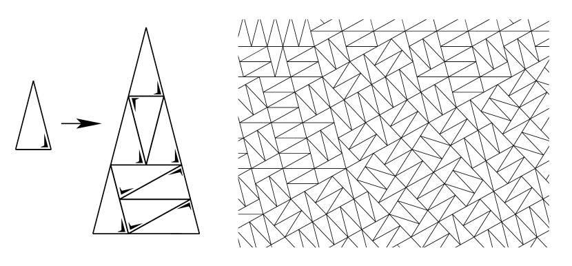
Figure 2. Another substitution rule which generates a tiling with circularly symmetric autocorrelation. The decoration of the triangles indicates that, in contrast to the classic pinwheel, no enantiomorphic pairs of triangles occur here.

Proposition 1.

The pinwheel Delone set $\varLambda$ as defined in Figure 1 satisfies:

• $\varLambda\subset\bigcup_{n\in\mathbb{Z}}R_{n\theta}\mathbb{Z}^{2}$, where $\theta:=2\arctan(\frac{1}{2})$.

• $\varLambda\subset\bigl{\{}(\textstyle{\frac{n}{5^{k}},\frac{m}{5^{k}}})\mid m,n\in\mathbb{Z},\;k\in\mathbb{N}_{0}\bigr{\}}$.

• The distance set ${\mathcal{D}}={\mathcal{D}}_{\varLambda}:=\{|x-y|\mid x,y\in\varLambda\}$ is a subset of $\bigl{\{}\sqrt{\frac{p^{2}+q^{2}}{5^{\ell}}}\mid p,q,\ell\in\mathbb{N}_{0}\bigr{\}}$.

In plain words, $\varLambda$ is a uniformly discrete subset of a countable union of rotated square lattices, all elements of $\varLambda$ have rational coordinates, and, as a consequence, all squared distances between points in $\varLambda$ are rational numbers of the form $(p^{2}+q^{2})/5^{\ell}$. The fact that $\varLambda$ is supported on such a simple set is an interesting property of the pinwheel tiling. It is not clear whether a similar property, for a suitable choice of control points, can be expected for other examples, such as that of Figure 2.

These results were obtained by means of an alternative substitution, the kite domino substitution shown in Figure 3, which generates the same Delone set $\varLambda$. The kite domino substitution is equivalent to the pinwheel substitution in the sense that the corresponding tilings are mutually locally derivable (MLD) in the sense of [4], i.e., they can be obtained from each other by local replacement rules. Moreover, the Delone set $\varLambda$ is MLD with both tilings.

Because of the strong linkage between the diffraction spectrum of a Delone set $\varLambda$ and the dynamical spectrum of the associated dynamical system $(\mathbb{X}(\varLambda),\mathbb{R}^{d})$, we consider the hull of $\varLambda$

$$\mathbb{X}(\varLambda)\;=\;\overline{\mathbb{R}^{2}+\varLambda}^{\,\sf LRT},$$

where completion is with respect to the local rubber topology (LRT), see [3] and references therein for details. Roughly speaking, and restricted to the special case under consideration, this means that $\mathbb{X}(\varLambda)$ contains all translates of $\varLambda$ and all Delone sets which are locally congruent to some translate of $\varLambda$.

In addition to Proposition 1, the kite domino substitution gives access also to the frequency of configurations in the tilings. The frequency of a finite set $L\subset\varLambda$ is defined as

$$\text{freq}(L)\;=\;\lim_{R\to\infty}\frac{1}{\pi R^{2}}\;\text{card}\{F\subset\varLambda\cap B_{R}\mid F\;\text{is congruent to}\;L\}.$$

Note that this definition is up to congruence of the finite sets, not up to translation (which is not reasonable here). The frequency module of $\varLambda$ is the $\mathbb{Z}$-span of $\{\text{freq}(L)\mid L\subset\varLambda\;\text{finite}\}$.

Figure 3. The kite domino substitution rule and a patch of a kite domino tiling. This patch is equivalent to the pinwheel patch in Figure 1. The dots in the patch indicate how $\varLambda$ arises from the tiling.

Proposition 2.

The frequency module of $\varLambda$ is $\{\frac{m}{264\cdot 5^{\ell}}\mid m\in\mathbb{Z},\,\ell\in\mathbb{N}_{0}\}$. It is the same for all elements of $\mathbb{X}(\varLambda)$. In particular, all $\eta(r)$ in (2) are rational.

Using the kite domino substitution, one can determine some frequencies of small distances exactly. These are given below, together with some other values (marked by an asterisk) where the frequencies are estimated by analysing large approximants of the pinwheel tiling.

(3) $$\begin{array}[]{l||c|c|c|c|c|c|c|c|c|c|c|c|c}\rule[-5.69054pt]{0.0pt}{19.91692pt}r^{2}&\;0&\frac{1}{5}&1&\;\frac{8}{5}&\frac{9}{5}&\frac{49}{25}&2&\frac{13}{5}&\frac{81}{25}&\frac{17}{5}&4&\frac{113}{25}&5\\ \hline\cr\rule[-5.69054pt]{0.0pt}{19.91692pt}\eta(r)&1&\frac{5}{11}&\frac{439}{165}&\frac{1}{2}&\frac{67}{165}&\frac{4}{165}&\frac{7}{2}^{\ast}&\frac{142}{165}&\frac{4}{165}&\frac{10}{11}^{\ast}&3^{\ast}&\frac{8}{165}^{\ast}&\frac{73}{15}^{\ast}\end{array}$$

By using ‘collared’ tiles (which refers to the ‘border-forcing’ property of [11]), one can in principle derive all frequencies in ${\mathcal{D}}$, see [8]. In fact, the frequency of pairs of points with distance $r=1$ in the table above was calculated this way. However, the computation of each single frequency requires a considerable amount of work, and a closed formula for all frequencies seems out of reach.

2. Diffraction

The diffraction of a crystal which is supported on a point lattice in $\mathbb{R}^{d}$ is obtained by the Poisson summation formula for Dirac combs [5, 6]. If $\varGamma$ is a lattice, the autocorrelation of the lattice Dirac comb $\delta_{\varGamma}$ is $\text{dens}(\varGamma)\,\delta_{\varGamma}$, and the diffraction measure reads

(4) $$\widehat{\delta}_{\varGamma}\;=\;\bigl{(}\text{dens}(\varGamma)\bigr{)}^{2}\cdot\delta_{\varGamma^{\ast}},$$

where $\varGamma^{\ast}$ is the dual lattice of $\varGamma$.

A radial analogue of Eq. (4) is derived in [1]. It is an analogue of the Hardy-Landau-Voronoi formula [10] in terms of tempered distributions. Let us first explain this for the example of the square lattice $\mathbb{Z}^{2}$. Let ${\mathcal{D}}_{\scriptscriptstyle\square}$ be the distance set of $\mathbb{Z}^{2}$, and $\eta_{\scriptscriptstyle\square}(r):=\text{card}\{x\in\mathbb{Z}^{2}\mid|x|=r\}$ the shelling numbers of $\mathbb{Z}^{2}$, see [2] for details. Then

(5) $$\Bigl{(}\sum_{r\in{\mathcal{D}}_{\scriptscriptstyle\square}}\eta_{\scriptscriptstyle\square}(r)\,\mu_{r}\Bigr{)}^{\widehat{}}=\sum_{r\in{\mathcal{D}}_{\scriptscriptstyle\square}}\eta_{\scriptscriptstyle\square}(r)\,\widehat{\mu}_{r}=\sum_{r\in{\mathcal{D}}_{\scriptscriptstyle\square}}\eta_{\scriptscriptstyle\square}(r)\,\mu_{r},$$

with $\mu_{r}$ as above. Again, the sum is to be understood as a vague limit. The fact that $\mathbb{Z}^{2}$ is self-dual as a lattice (i.e., $(\mathbb{Z}^{2})^{\ast}=\mathbb{Z}^{2}$) implies that the same distance set enters all three sums in (5). In the general case, with an arbitrary lattice $\varGamma$, one has to use the distance set of the dual lattice $\varGamma^{\ast}$ of $\varGamma$, in analogy with (4). This gives the following result [1], valid in Euclidean space of arbitrary dimension.

Theorem 1.

Let $\varGamma$ be a lattice of full rank in $\mathbb{R}^{d}$, with dual lattice $\varGamma^{\ast}$. If the sets of radii for non-empty shells are ${\mathcal{D}}_{\varGamma}$ and ${\mathcal{D}}_{\varGamma^{\ast}}$, with shelling numbers $\eta_{\varGamma}(r)=\mathrm{card}\,\{x\in\varGamma\mid\lvert x\rvert=r\}$ and $\eta_{\varGamma^{\ast}}(r)$ defined analogously, the classical Poisson summation formula has the radial analogue

(6) $$\Bigl{(}\sum_{r\in{\mathcal{D}}_{\varGamma}}\eta_{\varGamma}(r)\,\mu_{r}\Bigr{)}^{\widehat{}}\;=\;\mathrm{dens}(\varGamma)\sum_{r\in{\mathcal{D}}_{\varGamma^{\ast}}}\eta_{\varGamma^{\ast}}(r)\,\mu_{r}\,,$$

where $\mu_{r}$ denotes the uniform probability measure on the sphere of radius $r$ around the origin.

Eq. (6) also implies

(7) $$\Bigl{(}\sum_{r\in{\mathcal{D}}_{\varGamma}}\eta_{\varGamma}(r)\,\mu_{r}\Bigr{)}^{\widehat{}}\;=\;\sum_{r\in{\mathcal{D}}_{\varGamma}}\eta_{\varGamma}(r)\,\widehat{\mu}_{r}$$

in the sense of tempered distributions. This equation is useful in numerical calculations of pinwheel diffraction spectra.

2.1. Pinwheel diffraction

Let us return to the pinwheel pattern $\varLambda$. In view of Eq. (2) in connection with Proposition 1, the sum in Eq. (2) can be recast into a double sum,

(8) $$\gamma\;=\;\sum_{\ell=0}^{\infty}\;\sum_{r\in 5^{-\ell/2}{\mathcal{D}}_{\scriptscriptstyle\square}}\eta_{\ell}(r)\,\mu_{r}\,,$$

where the choice of the $\eta_{\ell}(r)$ is not unique, but restricted by the condition $\sum_{\ell=0}^{\infty}\eta_{\ell}(r)=\eta(r)$. If the $\eta_{\ell}(r)$, for fixed $\ell$, could be chosen to be ‘lattice-like’ — in the sense that they form a sequence of shelling numbers for some lattice — we were in the position to apply Eq. (6) to each inner sum in Eq. (8) individually. Observing that

(9) $${\bigl{(}5^{-\ell/2}\,\mathbb{Z}^{2}\bigr{)}}^{\ast}\;=\;5^{\ell/2}\,\mathbb{Z}^{2}$$

this would give rise to terms of the form $\sum_{r\in 5^{\ell/2}{\mathcal{D}}_{\scriptscriptstyle\square}}\,\eta^{\,\prime}_{\ell}(r)\,\widehat{\mu}_{r}$. Due to the continuity of the Fourier transform on the space of tempered distributions, this would imply the diffraction of the pinwheel tiling to be purely singular.

However, things are not that simple in the case of the pinwheel tiling. In particular, the $\eta_{\ell}(r)$ cannot be chosen to be lattice-like, as a consequence of the Delone nature of $\varLambda$. Nevertheless, it may still be possible to find coefficients $\epsilon_{\ell}$, not necessarily positive, such that the autocorrelation of $\varLambda$ can be written as

$$\gamma\;=\;\sum_{\ell\geq 0}\epsilon_{\ell}\sum_{r\in 5^{-\ell/2}{\mathcal{D}}_{\scriptscriptstyle\square}}\eta_{\ell}(r)\,\mu_{r}\,.$$

This general form permits continuous parts in the diffraction different from the ones arising from (9): There may be singular continuous parts apart from $\{r\mathbb{S}^{1}\mid r\in{\mathcal{D}}\setminus\{0\}\}$, and even absolutely continuous parts. In fact, numerical computations indicate [1] the presence of an absolutely continuous part in the diffraction.

Independent of an affirmative answer of the open questions, there is a striking resemblance with the powder diffraction image of the square lattice. This is a consequence of Proposition 1. So let us close this article with a simplified approach to powder diffraction patterns, and a comparison of the two images.

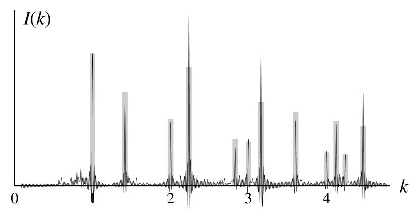
Figure 4. Numerical approximation to the radial intensity structure $I(k)$ of the pinwheel diffraction (solid line) in comparison with the powder diffraction structure of the square lattice (grey bars). The relative scale has been chosen such that the heights of the first peaks at $k=1$ match. Note that the central intensity is suppressed.

2.2. Square lattice powder diffraction

Instead of performing a diffraction experiment with a large single crystal, it is often easier to use a probe that comprises many grains in — ideally — random and mutually uncorrelated orientations [17]. This setting can be modelled mathematically as follows. Let $R$ be a rotation of infinite order, i.e., $R^{n}\neq\mathrm{id}$ for all integer $n\neq 0$. It follows from Weyl’s lemma that $\{R^{n}x\mid n\in\mathbb{N}_{0}\}$ is uniformly distributed on the unit circle $\mathbb{S}^{1}$ for any $x\in\mathbb{S}^{1}$. For simplicity, we require $R\mathbb{Z}^{2}\cap\mathbb{Z}^{2}=\{0\}$. Then, for large $N$, the set

$$\omega_{N}=\frac{1}{N}\bigcup_{j=1}^{N}R^{j}\mathbb{Z}^{2}$$

can serve as an idealised powder emerging from a two-dimensional crystal supported on $\mathbb{Z}^{2}$. Note that the prefactor $1/N$ appears because we idealise the arrangement of disoriented grains as an overlay of mutually rotated infinite copies of $\mathbb{Z}^{2}$.

It is not hard to show [1] that the corresponding autocorrelation is given by

$$\gamma_{\omega_{N}}=\frac{N-1}{N}\,\lambda+\frac{1}{N}\left(\frac{1}{N}\sum_{j=0}^{N-1}\delta_{R^{j}\mathbb{Z}^{2}}\right),$$

where $\lambda$ denotes Lebesgue measure in $\mathbb{R}^{2}$. The limit of the bracketed term, as $N\to\infty$, shows perfect circular symmetry, and is a reasonable approximation of the powder autocorrelation. An application of Theorem 1 or Eq. (5), yields

(10) $$\lim_{N\to\infty}\Bigl{(}\frac{1}{N}\sum_{j=0}^{N-1}\delta_{R^{j}\mathbb{Z}^{2}}\Bigr{)}^{\widehat{}}\;=\;\Bigl{(}\sum_{r\in{\mathcal{D}}_{\scriptscriptstyle\square}}\eta_{\scriptscriptstyle\square}(r)\,\mu_{r}\Bigr{)}^{\widehat{}}\;=\;\sum_{r\in{\mathcal{D}}_{\scriptscriptstyle\square}}\eta_{\scriptscriptstyle\square}(r)\,\mu_{r}\,.$$

This shows that, for an ideal square lattice powder as above, one can expect a diffraction image that, beyond the central intensity, consists of concentric rings of radius $r\in{\mathcal{D}}_{\scriptscriptstyle\square}$ with total intensity $\eta_{\scriptscriptstyle\square}(r)$. In this simplified version, there is no absolutely continuous part, though this would be present in a more realistic model.

To compare the powder diffraction of $\mathbb{Z}^{2}$ with the pinwheel diffraction, we note that it is sufficient to display the radial structure. Furthermore, we cannot compare the central intensity, wherefore we suppress it in both cases. While Eq. (10) gives a closed formula for the intensity of the rings in the powder diffraction, we currently only have a numerical approximation to the pinwheel diffraction, based on Eq. (7) and a large patch, see [1] for details. Figure 4, which speaks for itself, shows striking similarities of the singular parts. It is thus plausible that further investigations in this direction might ultimately reveal the full nature of the pinwheel diffraction.

References

- [1] M. Baake, D. Frettlöh and U. Grimm, A radial analogue of Poisson’s summation formula with applications to powder diffraction and pinwheel patterns, preprint (2006).
- [2] M. Baake and U. Grimm, A note on shelling, Discrete Comput. Geom. 30, 573–589 (2003); math.MG/0203025.
- [3] M. Baake and D. Lenz, Dynamical systems on translation bounded measures: Pure point dynamical and diffraction spectra, Ergodic Th. & Dynam. Syst. 24, 1867–1893 (2004); math.DS/0302231.
- [4] M. Baake, M. Schlottmann and P. D. Jarvis, Quasiperiodic patterns with tenfold symmetry and equivalence with respect to local derivability, J. Phys. A: Math. Gen. 24, 4637–4654 (1991).
- [5] A. Córdoba, La formule sommatoire de Poisson, C. R. Acad. Sci. Paris, Sér. I: Math. 306, 373–376 (1988).
- [6] A. Córdoba, Dirac combs, Lett. Math. Phys. 17, 191–196 (1989).
- [7] D. Frettlöh and E. Harriss, Tilings Encyclopedia, available online at: http://tilings.math.uni-bielefeld.de
- [8] D. Frettlöh and M. Whittaker, in preparation.
- [9] A. Hof, On diffraction by aperiodic structures, Commun. Math. Phys. 169, 25–43 (1995).
- [10] H. Iwaniec and E. Kowalski, Analytic Number Theory, AMS, Providence, RI (2004).
- [11] J. Kellendonk, Topological equivalence of tilings, J. Math. Phys. 38, 1823–1842 (1997).
- [12] R. V. Moody, D. Postnikoff and N. Strungaru, Circular symmetry of pinwheel diffraction, Ann. H. Poincaré 7, 711–730 (2006).
- [13] N. Ormes, C. Radin and L. Sadun, A homeomorphism invariant for substitution tiling spaces, Geom. Dedicata 90, 153–182 (2002).
- [14] C. Radin, The pinwheel tilings of the plane, Annals Math. 139, 661–702 (1994).
- [15] L. Sadun, Some generalizations of the pinwheel tiling, Discrete Comput. Geom. 20, 79–110 (1998).
- [16] M. Schlottmann, Generalized model sets and dynamical systems, in: Directions in Mathematical Quasicrystals, eds. M. Baake and R. V. Moody (CRM Monograph Series, vol.13, AMS, Providence, RI, 2000), pp. 143–159.
- [17] B. E. Warren, X-ray Diffraction, reprint, Dover, New York (1990).
- [18] T. Yokonuma, Discrete sets and associated dynamical systems in a non-commutative setting, Canad. Math. Bull. 48, 302–316 (2005).