$\mathcal{P}\mathcal{T}$-Symmetric Extension of the Korteweg-de Vries Equation

Abstract

The Korteweg-de Vries equation $u_{t}+uu_{x}+u_{xxx}=0$ is $\mathcal{P}\mathcal{T}$ symmetric (invariant under space-time reflection). Therefore, it can be generalized and extended into the complex domain in such a way as to preserve the $\mathcal{P}\mathcal{T}$ symmetry. The result is the family of complex nonlinear wave equations $u_{t}-iu(iu_{x})^{\epsilon}+u_{xxx}=0$, where $\epsilon$ is real. The features of these equations are discussed. Special attention is given to the $\epsilon=3$ equation, for which conservation laws are derived and solitary waves are investigated.

preprint LA-UR-06-6952

Many papers have been written on theories described by non-Hermitian $\mathcal{P}\mathcal{T}$-symmetric quantum-mechanical Hamiltonians. To construct such theories one begins with a Hamiltonian that is both Hermitian and $\mathcal{P}\mathcal{T}$ symmetric, such as the harmonic oscillator $H=p^{2}+x^{2}$. One then introduces a real parameter $\epsilon$ to extend the Hamiltonian into the complex domain in such a way as to preserve the $\mathcal{P}\mathcal{T}$ symmetry:

$$H=p^{2}+x^{2}(ix)^{\epsilon}.$$ (1)

The result is a family of complex non-Hermitian Hamiltonians that for positive $\epsilon$ maintain many of the properties of the harmonic oscillator Hamiltonian; namely, that the eigenvalues remain real, positive, and discrete [1, 2, 3]. The properties of classical $\mathcal{P}\mathcal{T}$-symmetric Hamiltonians have also been examined [4, 5, 6, 7]. However, there are to date no published studies of $\mathcal{P}\mathcal{T}$-symmetric classical wave equations.

The starting point of this paper is the heretofore unnoticed property that the Korteweg-de Vries (KdV) equation,

$$u_{t}+uu_{x}+u_{xxx}=0,$$ (2)

is $\mathcal{P}\mathcal{T}$ symmetric. To demonstrate this, we define parity reflection $\mathcal{P}$ by $x\to-x$, and since $u=u(x,t)$ is a velocity, the sign of $u$ also changes under $\mathcal{P}$: $u\to-u$. We define time reversal $\mathcal{T}$ by $t\to-t$, and again, since $u$ is a velocity, the sign of $u$ also changes under $\mathcal{T}$: $u\to-u$. Following the quantum-mechanical formalism, we also require that $i\to-i$ under time reversal. It is clear that the KdV equation is not symmetric under $\mathcal{P}$ or $\mathcal{T}$ separately, but it is symmetric under combined $\mathcal{P}\mathcal{T}$ reflection. The KdV equation is a special case of the Camassa-Holm equation [8], which is also $\mathcal{P}\mathcal{T}$ symmetric. Other nonlinear wave equations such as the generalized KdV equation $u_{t}+u^{k}u_{x}+u_{xxx}=0$ and the Sine-Gordon equation $u_{tt}-u_{xx}+g\sin u=0$ are $\mathcal{P}\mathcal{T}$ symmetric as well.

The striking observation that there are many nonlinear wave equations possessing $\mathcal{P}\mathcal{T}$ symmetry suggests that one can generate many families of new complex nonlinear $\mathcal{P}\mathcal{T}$-symmetric wave equations by following the same procedure that was used in quantum mechanics [see (1)]. One should then try to discover which properties of the original wave equations are preserved.

In this brief note we limit our discussion to the complex $\mathcal{P}\mathcal{T}$-symmetric extension of the KdV equation:

$$u_{t}-iu(iu_{x})^{\epsilon}+u_{xxx}=0,$$ (3)

where $\epsilon$ is a real parameter. We now examine the remarkable properties of some members of this family of complex $\mathcal{P}\mathcal{T}$-symmetric equations. We will emphasize the properties that members of this class have in common.

Case $\epsilon=1$: When $\epsilon=1$, (3) reduces to the KdV equation (2). The KdV equation has an infinite number of conserved quantities [9]. The first two are the momentum $P$,

$$\frac{d}{dt}P=0,\qquad P=\int dx\,u(x,t),$$ (4)

and the energy $E$,

$$\frac{d}{dt}E=0,\qquad E=\mbox{$\textstyle{\frac{1}{2}}$}\int dx\,[u(x,t)]^{2}.$$ (5)

The Cauchy initial-value problem for the KdV equation can be solved exactly because the system is integrable, and it is solved by using the method of inverse scattering [10].

A solitary-wave solution to the KdV equation has the form

$$u(x,t)=3c\,{\rm sech}^{2}\left[\mbox{$\textstyle{\frac{1}{2}}$}\sqrt{c}\left(x-ct-x_{0}\right)\right],$$ (6)

where $c>0$ is the velocity. (In general, a solitary-wave solution $u(x,t)=f(x-ct)$ to a partial differential equation is defined to be a wave that propagates at constant velocity $c$ and whose shape does not change in time. In this paper we also require that $f(z)\to 0$ as $|z|\to\infty$.) These solitary waves are called solitons because as they evolve according to the KdV equation they retain their shape when they undergo collisions with other solitary waves. One can observe numerically how a soliton emerges from a pulse-like initial condition. For example, for the initial condition $u(x,0)=3\,{\rm sech}(x)$, we see in Fig. 1 that the pulse sheds a stream of wave-like radiation that travels to the left and gives birth to a right-moving soliton of the form in (6).

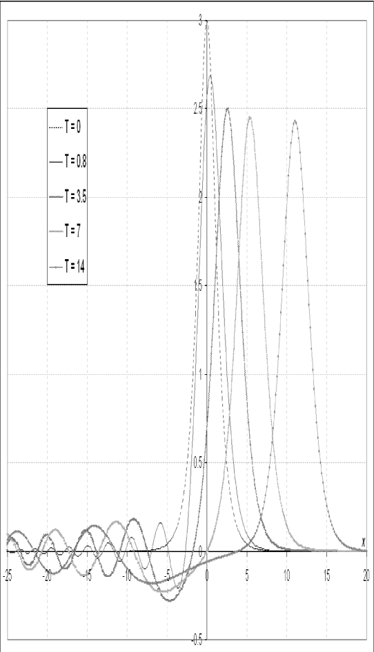
Figure 1: Birth of a soliton. As the initial condition $u(x,0)=3\,{\rm sech}(x)$ evolves in time according to the KdV equation, a soliton of the form (6) moves to the right leaving a trail of residual radiation that propagates to the left. The function $u(x,T)$ is plotted for $T=0$, $0.8$, $3.5$, $7$, and $14$.

Case $\epsilon=0$: Setting $\epsilon=0$ in (3) gives the linear equation

$$u_{t}-iu+u_{xxx}=0.$$ (7)

To solve the initial-value problem for this equation, we substitute $u(x,t)=e^{it}v(x,t)$ and reduce it to $v_{t}+v_{xxx}=0$. We then perform a Fourier transform to obtain the solution in the form of a convolution of the initial condition and an inverse Fourier transform:

$$v(x,t)=v(x,0)\ast{\cal F}^{-1}\left(e^{ip^{3}t}\right).$$ (8)

The inverse Fourier transform of the exponential of a cubic is an Airy function [11]. Thus, the exact solution for $u(x,t)$ is

$$u(x,t)=e^{it}(3t)^{-1/3}\int_{-\infty}^{\infty}ds\,u(x-s,0){\rm Ai}\left[(3t)^{-1/3}s\right].$$ (9)

The Airy function ${\rm Ai}(x)$ has a global maximum near $x=0$. For $x$ large and positive ${\rm Ai}(x)$ decays exponentially, ${\rm Ai}(x)\sim(2\sqrt{\pi})^{-1}x^{-1/4}\exp\left(-\frac{2}{3}x^{3/2}\right)$, and for $x$ large and negative ${\rm Ai}(x)$ decays algebraically and oscillates, ${\rm Ai}(-x)\sim\pi^{-1/2}x^{-1/4}\sin\left(\frac{2}{3}x^{3/2}+\frac{1}{4}\pi\right)$. Thus, the qualitative behavior of ${\rm Ai}(x)$ resembles that in Fig. 1. If we choose the initial condition $u(x,0)=3\,{\rm sech}(x)$ that was used to generate Fig. 1, then apart from the phase $e^{it}$, we find that the solution (9), which is shown in Fig. 2, resembles that for the KdV equation in Fig. 1 except that no soliton emerges from the initial condition. There is only residual radiation that travels to the left. Thus we have extended the KdV equation into the complex domain while preserving many of its qualitative features.

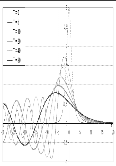
Figure 2: Plot of $u(x,T)e^{-iT}$ as a function of $x$ for $T=0$, $5$, $10$, $20$, $40$, and $80$, where $u(x,t)$ in (9) is calculated for the initial condition $u(x,0)=3\,{\rm sech}(x)$. A comparison of this figure with Fig. 1 shows that the solutions to (3) with $\epsilon=0$ and $\epsilon=1$ are somewhat similar. However, in this case, while the initial condition produces radiation that travels to the left, it does not give rise to a soliton.

Case $\epsilon=3$: If we set $\epsilon=3$ in (3), we obtain the nonlinear wave equation

$$u_{t}-u(u_{x})^{3}+u_{xxx}=0,$$ (10)

which has received only passing mention in the literature [12, 13]. The only observations that have been made regarding this equation are that, apart from translation invariance in $x$ and $t$, there is an obvious scaling solution of the form $u(x,t)=\phi\left(xt^{-1/3}\right)$. Yet, this equation has an array of rich and beautiful properties that have so far been overlooked. As we will show, there are two conserved quantities, a momentum $P$ and an energy $E$, which are the analogs of $P$ and $E$ in (4) and (5) for the KdV equation. We will also show that there are traveling waves, and we will see how a pulse-like initial condition gives birth to a traveling wave, just as in the case of the KdV equation.

We derive the conserved quantities for the wave equation (10) in much the same way that one finds the conserved quantities for the KdV equation (2). However, the procedure is more elaborate. To find the momentum $P$, we begin by integrating (10) with respect to $x$ and assume that $u(x,t)$ vanishes rapidly as $|x|\to\infty$. For the case of the KdV equation, this procedure immediately gives the result in (4). However, for the equation in (10) we have the result

$$\frac{d}{dt}\int dx\,u=\int dx\,u(u_{x})^{3}.$$ (11)

Evidently, $\int u$ is not a conserved quantity because the right side of of this equation does not vanish (in contrast to the KdV equation). To proceed we introduce the identity

$$\int dx\,u^{N}(u_{x})^{3}=\frac{2}{(N+1)(N+2)}\int dx\,u^{N+2}u_{xxx},$$ (12)

which is obtained by performing two integrations by parts. Using this identity for the case $N=1$, we rewrite (11) as

$$\frac{d}{dt}\int dx\,u=\frac{1}{3}\int dx\,u^{3}u_{xxx}.$$ (13)

This equation suggests that we should multiply (10) by $u^{3}$, integrate with respect to $x$, and use the identity (12) for the case $N=4$ to obtain

$$\frac{1}{4}\,\frac{d}{dt}\int dx\,u^{4}=\frac{1}{15}\int dx\,u^{6}u_{xxx}-\int dx\,u^{3}u_{xxx}.$$ (14)

We can combine (13) and (14) to eliminate the $\int u^{3}u_{xxx}$ term, but the right side will still not vanish because there will be a $\int u^{6}u_{xxx}$ term.

Therefore, we must iterate this process by multiplying by $u^{6}$, $u^{9}$, $u^{12}$, and so on, and then integrating with respect to $x$. We thus obtain the following sequence of equations:

$$\frac{d}{dt}\int dx\,\frac{u^{3k+1}}{3k+1}=\int dx\,\frac{2u^{3k+3}u_{xxx}}{(3k+2)(3k+3)}-\int dx\,u^{3k}u_{xxx},$$ (15)

where $k=0,1,2,3,\cdots$. We can now completely eliminate the right side if we multiply the $k$th equation in (15) by

$$a_{k}=\frac{6^{k}\Gamma\left(k+\frac{1}{3}\right)}{(3k)!}A,$$ (16)

where $A$ is an arbitrary constant, and sum from $k=0$ to $\infty$. We conclude that $\frac{d}{dt}P=0$, where the conserved quantity $P$ is given by

$$P=A\int dx\sum_{k=0}^{\infty}\frac{6^{k}\Gamma\left(k+\frac{1}{3}\right)u^{3k+1}}{(3k+1)!}.$$ (17)

By a similar argument, we can construct a second conserved quantity $E$, $\frac{d}{dt}E=0$, where $E$ is given by

$$E=B\int dx\sum_{k=0}^{\infty}\frac{6^{k}\Gamma\left(k+\frac{2}{3}\right)u^{3k+2}}{(3k+2)!}$$ (18)

and $B$ is an arbitrary constant.

The summations in (17) and (18) can be performed in closed form in terms of Airy functions, giving

$$P = \int dx\,\int_{0}^{2^{1/3}u(x,t)}ds\,\left[{\rm Bi}(s)+\sqrt{3}{\rm Ai}(s)\right],$$

$$E = \int dx\,\int_{0}^{2^{1/3}u(x,t)}ds\,\left[{\rm Bi}(s)-\sqrt{3}{\rm Ai}(s)\right],$$ (19)

where we have taken $A=6^{1/3}/\pi$ and $B=6^{2/3}/\pi$. It is especially noteworthy that the conserved quantity $E$ is strictly positive when $u(x,t)$ is not identically 0, and thus it is reasonable to interpret $E$ as an energy. The positivity property of the energy is maintained when $\epsilon$ changes from 1 (the KdV equation) to 3. We do not believe that (10) has more than two conserved quantities.

Equation (10) is also similar to the KdV equation in that it has solitary-wave solutions. To construct such a solution, we substitute $u(x,t)=f(x-ct)$ into (10) to find the ordinary differential equation satisfied by $f(z)$:

$$-cf^{\prime}(z)-f(z)[f^{\prime}(z)]^{3}+f^{\prime\prime\prime}(z)=0.$$ (20)

It is only possible to solve this autonomous equation in implicit form. To do so, we seek a solution of the form $f^{\prime}(z)=G(f)$. The function $G$ satisfies

$$-2c-2fG^{2}(f)+\left[G^{2}(f)\right]^{\prime\prime}=0.$$ (21)

Making the further substitution $H(f)=G^{2}(f)$, we find that $H$ satisfies

$$H^{\prime\prime}(f)-2fH(f)=2c,$$ (22)

which is the inhomogeneous Airy equation, whose solution is expressed in terms of the inhomogeneous Airy or Scorer function ${\rm Hi}$ [11].

Unfortunately, because the solution to (20) is implicit, it is not easy to determine immediately whether there are solitary-wave solutions [solutions $f(z)$ that vanish as $|z|\to\infty$]. However, numerical analysis confirms that there are indeed such solutions. In Fig. 3 we have plotted the solitary wave for $c=1$. Note that this wave is an even function of $z$ and it decays like $e^{-|z|}$ for large $|z|$. Note also that the solitary-wave solution is a negative pulse, rather than a positive pulse as with the KdV equation.

Figure 3: Solitary-wave solution to the differential equation $u_{t}-u(u_{x})^{3}+u_{xxx}=0$. This negative-pulse solution has the form $u(x,t)=f(x-ct)$, where we have taken $c=1$. The solitary wave is an even function of $z=x-t$ and it decays like $e^{-|z|}$ for large $|z|$. Thus, it closely resembles the solitary-wave solution in (6) for the KdV equation. At the negative peak the height of this solitary wave is $-2.73802$.

As we saw in Fig. 1 for the KdV equation, an initial pulse such as $u(x,0)=-3\,{\rm sech}(x)$ for (10) gives birth to a solitary wave. As shown in Fig. 4, this initial pulse emits radiation that travels to the left and evolves into a right-going solitary wave (see Fig. 3). Computer experiments suggest that these solitary waves are not solitons; that is, they do not maintain their shape after a collision with another solitary wave. Indeed, we would be surprised if (10) were an integrable system. The quantum-mechanical Hamiltonian(1) ceases to be exactly solvable when $\epsilon\neq 0$, and in the same vein we expect that (3) is not integrable when $\epsilon\neq 0$.

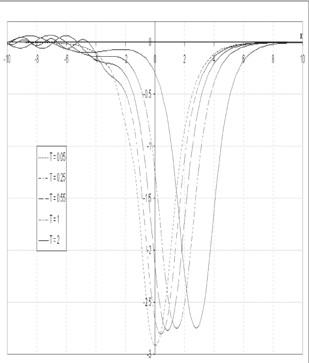
Figure 4: Birth of a solitary wave. As the initial condition $u(x,0)=-3\,{\rm sech}(x)$ evolves in time according to $u_{t}-u(u_{x})^{3}+u_{xxx}=0$, a pulse that approaches the shape of a solitary wave moves to the right leaving a trail of residual radiation that propagates to the left. The wave $u(x,T)$ is shown for the times $T=0.05,\,0.25,\,0.55,\,1,\,{\rm and}\,2$.

There are no positive solitary-wave solutions to (10). As we see in Fig. 5, an initial pulse of the form $u(x,0)=3\,{\rm sech}(x)$ generates a stream of radiation that travels to the left, but it does not give rise to a solitary wave.

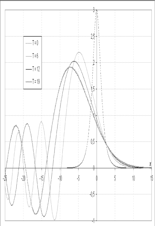
Figure 5: The solution to $u_{t}-u(u_{x})^{3}+u_{xxx}=0$ that evolves from the initial condition $u(x,0)=3\,{\rm sech}(x)$. This initial condition generates radiation that travels to the left, but it does not give rise to a solitary wave. The wave $u(x,T)$ is shown for the times $T=0,\,6,\,12,\,{\rm and}\,19$.

Case $\epsilon=2n+1$: When $\epsilon=2n+1$ is an odd integer, the nonlinear wave equation in (3) is real:

$$u_{t}+(-1)^{n}u(u_{x})^{2n+1}+u_{xxx}=0.$$ (23)

For all values of $n$ there are solitary waves $u(x,t)=f(z)$, where $z=x-ct$, and these waves are even functions of $z$. As $n$ increases, the solitary waves alternate between being strictly positive and strictly negative functions and gradually become wider (see Fig. 6).

Figure 6: Solitary-wave solutions of the form $f(x-t)$ to the differential equation $u_{t}+(-1)^{n}u(u_{x})^{2n+1}+u_{xxx}=0$ for $n=1,2,3,4$. Note that the solutions are alternately positive and negative and gradually get wider as $n$ increases. At the stationary points the heights of the waves are $-2.73802$ ($n=1$), $2.45839$ ($n=2$), $-2.30305$ ($n=3$), and $2.20797$ ($n=4$). The widths of the waves at half-height are $3.15$, $3.14$, $3.19$, and $3.26$, respectively.

In conclusion, we have shown how to extend the conventional KdV equation into the complex domain while preserving $\mathcal{P}\mathcal{T}$ symmetry. The result is a large and rich class of nonlinear wave equations that share many of the properties of the KdV equation. In particular, we find that for some values of $\epsilon$ there are conservation laws and solitary waves, and that arbitrary initial pulses can evolve into solitary waves after they give off a stream of radiation. Airy functions appear repeatedly in the analysis because the associated linear equation that is satisfied when $u(x,t)$ is small is of Airy type.

In this paper we have just scratched the surface; one can begin with other $\mathcal{P}\mathcal{T}$-symmetric nonlinear wave equations, such as the Camassa-Holm or the generalized KdV equations, and study the properties of the resulting new complex wave equations.

We thank P. Clarkson, D. Holm, H. Jones, and B. Muratori for useful discussions. CMB is grateful to the Theoretical Physics Group at Imperial College, London, for its hospitality. As an Ulam Scholar, CMB receives financial support from the Center for Nonlinear Studies at the Los Alamos National Laboratory and he is supported in part by a grant from the U.S. Department of Energy. DCB is supported by The Royal Society.

References

- [1] C. M. Bender and S. Boettcher, Phys. Rev. Lett. 80, 5243 (1998).
- [2] C. M. Bender, S. Boettcher, and P. N. Meisinger, J. Math. Phys. 40, 2201 (1999).
- [3] P. Dorey, C. Dunning and R. Tateo, J. Phys. A: Math. Gen. 34, L391 (2001); ibid. 34, 5679 (2001).
- [4] A. Nanayakkara, Czech. J. Phys. 54, 101 (2004) and J. Phys. A: Math. Gen. 37, 4321 (2004).
- [5] C. M. Bender, J.-H. Chen, D. W. Darg, and K. A. Milton, J. Phys. A: Math. Gen. 39, 4219-4238 (2006).
- [6] C. M. Bender and D. W. Darg (in preparation).
- [7] C. M. Bender, D. D. Holm, and D. W. Hook, [arXiv: math-ph/0609068].
- [8] R. Camassa and D. D. Holm, Phys. Rev. Lett. 71, 1661 (1993).
- [9] R. M. Miura, C. S. Gardner, and M. D. Kruskal, J. Math. Phys. 9, 1204 (1968).
- [10] G. B.Whitham, Linear and Nonlinear Waves (Wiley, New York, 1974).
- [11] M. Abramowitz and I. A. Stegun, Handbook of Mathematical Functions (Dover, New York, 1965), pp. 446-447.
- [12] A. D. Polyanin and V. F. Zaitsev, Handbook of Nonlinear Partial Differential Equations (Chapman & Hall/CRC, Boca Raton, 2004), pp. 526 and 529.
- [13] W. I. Fushchych, N. I. Serov, and T. K. Ahmerov, Rep. Ukr. Acad. Sci. A 12, 28 (1991).