Laminated Wave Turbulence: Generic Algorithms I

Abstract

The model of laminated wave turbulence presented recently unites both types of turbulent wave systems - statistical wave turbulence (introduced by Kolmogorov and brought to the present form by numerous works of Zakharov and his scientific school since nineteen sixties) and discrete wave turbulence (developed in the works of Kartashova in nineteen nineties). The main new feature described by this model is the following: discrete effects do appear not only in the long-wave part of the spectral domain (corresponding to small wave numbers) but all through the spectra thus putting forth a novel problem - construction of fast algorithms for computations in integers of order $10^{12}$ and more. In this paper we present a generic algorithm for polynomial dispersion functions and illustrate it by application to gravity and planetary waves.

Math. Classification: 76F02, 65H10, 65Yxx, 68Q25

Key Words: Laminated wave turbulence, discrete wave systems, computations in integers, transcendental algebraic equations, complexity of algorithm

Address:

Dr. Elena Kartashova

RISC, J. Kepler University

Altenbergerstr. 69

4020 Linz

Austria

e-mail: lena@risc.uni-linz.ac.at

Tel.: +42 (0)732 2468 9929

Fax: +42 (0)732 2468 9930

1 INTRODUCTION

Statistical theory of wave turbulence begins with the pioneering paper [1] of Kolmogorov presenting the energy spectrum of turbulence as a function of vortex size and thus founding the field of mathematical analysis of turbulence. Kolmogorov regarded some inertial range of wave numbers between viscosity and dissipation, $k_{0}<k<k_{1}$ for wave numbers $k$ where $k=|\vec{k}|$, and suggested that in this range turbulence is locally homogeneous and isotropic which, together with dimensional analysis, allowed Kolmogorov to deduce that energy distribution is proportional to $k^{-5/3}.$

Kolmogorov’s ideas were further applied by Zakharov for construction of wave kinetic equations [2] which are approximately equivalent to the initial nonlinear PDEs:

$$\dot{A}_{1}=\int|V_{(123)}|^{2}\delta(\omega_{1}-\omega_{2}-\omega_{3})\delta(\vec{k}_{1}-\vec{k}_{2}-\vec{k}_{3})(A_{2}A_{3}-A_{1}A_{2}-A_{1}A_{3}){\bf d}\vec{k}_{2}{\bf d}\vec{k}_{3}$$

for 3-wave interactions, and similar equations for $i$-wave interactions where $\delta$ is the Dirac delta-function and $V_{(12..i)}$ is the vortex coefficient in the standard representation of nonlinearity in the initial PDE:

$$\Sigma_{i}\frac{V_{(12..i)}\delta(\vec{k}_{1}+\vec{k}_{2}+...+\vec{k}_{i})}{\delta(\omega_{1}+\omega_{2}+...+\omega_{i})}A_{1}A_{2}\cdots A_{i}.$$ (1)

The main idea of the wave turbulence theory is to take into account only resonant interactions of waves described by

$$\begin{cases}\omega(\vec{k}_{1})\pm\omega(\vec{k}_{2})\pm...\pm\omega(\vec{k}_{n+1})=0,\\ \vec{k}_{1}\pm\vec{k}_{2}\pm...\pm\vec{k}_{n+1}=0\end{cases}$$ (2)

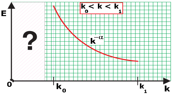
Figure 1: Statistical Wave Turbulence Theory, $|\vec{k}|>k_{0}$: Dependence of the energy $E$ on the wave number $k$ is presented in the right part of the picture; ZK-energy spectrum is shown symbolically. Left part of the picture is not explained by statistical wave turbulence theory.

Statistical wave turbulence theory deals with real solutions of Sys.(2) and one of its most important discoveries in the statistical wave turbulence theory are stationary exact solutions of the kinetic equations first found in [3]. These solutions have the form $k^{-\alpha}$ with $\alpha>0$ and are now called Zakharov-Kolmogorov (ZK) energy spectra (see Fig.1).

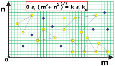
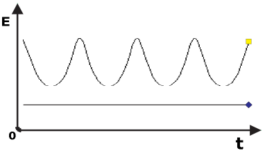
Figure 2: Discrete Wave Turbulence Theory, $|\vec{k}|<k_{0}$: 2D-spectral space is shown on the left panel, each node $(n,m)$ of integer lattice corresponds to the wave vector $\vec{k}=(n,m).$ Nodes corresponding to resonantly interacting waves are depicted by yellow squares and to non-interacting waves - by blue diamonds. On the right panel, dependence of the energy $E$ on time $t$ for both types of waves is shown

The left part of Fig.1, the so-called finite length effects, have been studied in the papers of Kartashova [4] where properties of integer solutions of Sys.(2) have been studied. It was proven in particular that the spectral space of the discrete wave system is decomposed into the small disjoint groups of waves showing periodic energy fluctuations (nodes connected by lines at the right panel of Fig. 2) and many waves with constant energy, depicted by blue diamonds.

The most important result of the theory of laminated wave turbulence [5] is following: discrete effects do appear not only in the long-wave part of the spectral space (corresponding to small wave numbers) but all along the wave spectra. From the computational point of view this theory gives rise to a completely novel problem: construction of fast algorithms for computations of integer solutions of Sys.(2) in integers of order $10^{1}2$ and more. For instance, for 4-wave interactions of 2-dimensional gravity waves this system has the form

$$\sqrt{k_{1}}+\sqrt{k_{2}}=\sqrt{k_{3}}+\sqrt{k_{4}},\quad\vec{k}_{1}+\vec{k}_{2}=\vec{k}_{3}+\vec{k}_{4},$$

where $\vec{k}_{i}=(m_{i},n_{i}),\ \forall i=1,2,3,4$ and $k_{i}=|\vec{k}_{i}|=\sqrt{m_{i}^{2}+n_{i}^{2}}$. It means that in a finite but big enough domain of wave numbers, say $|m|,|n|\leq D\sim 1000$, direct approach leads to necessity to perform extensive (computational complexity $D^{8}$) computations with integers of the order of $10^{12}$.

Importance of the discrete layer of laminated turbulence is emphasized by the fact that there exist many wave systems described only by discrete waves approach (for instance, wave systems with periodic or zero boundary conditions). A sketch of the first algorithm for the problems of laminated turbulence is given in [6].

In this paper we present generic algorithm for computing discrete layers of wave turbulent systems with dispersion function being a function of the modulus of the wave vector $\vec{k}$, $\omega=\omega(k)$. The main idea underlying our algorithm is the partition of the spectral space into disjoint classes of vectors which allows us to look for the solutions of Sys.(2) in each class separately. In Sec.2 we describe this construction in detail and with numerous examples because its brief description given in [7] is often misunderstood by other researchers. In Sec. 3 the generic algorithm is presented with gravity waves taken as our main example while in Sec. 4 modification of this algorithm is given for the oceanic planetary waves. Results of the computations and brief discussion are given at the end.

2 DEFINITION of CLASSES

For a given $c\in\hbox{\Sets N},c\neq 0,1,-1$ consider the set of algebraic numbers $R_{c}={\pm k^{1/c},k\in\hbox{\Sets N}}$. Any such number $k_{c}$ has a unique representation

$$k_{c}=\gamma q^{1/c},\gamma\in\hbox{\Sets Z}$$

where $q$ is a product

$$q=p_{1}^{e_{1}}p_{2}^{e_{2}}...p_{n}^{e_{n}},$$

while $p_{1},...p_{n}$ are all different primes and the powers $e_{1},...e_{n}\in\hbox{\Sets N}$ are all smaller than $c$.

Definition.

The set of numbers from $R_{c}$ having the same $q$ is called $q$-class $Cl_{q}$ (also called ”class $q$”). The number $q$ is called class index. For a number $k_{(c)}=\gamma q^{1/c}$, $\gamma$ is called the weight of $k_{(c)}$.

The following two Lemmas are easily obtained from elementary properties of algebraic numbers.

Lemma 1.

For any two numbers $k_{1},k_{2}$ belonging to the same $q$-class, all their linear combinations

$$a_{1}k_{1}+a_{2}k_{2},\quad a_{1},a_{2}\in\hbox{\Sets Z}$$

with integer coefficients belong to the same class $q$.

Indeed, if $k_{1}=\gamma_{1}q^{1/c},k_{2}=\gamma_{2}q^{1/c}$ then

$$a_{1}k_{1}+a_{2}k_{2}=\gamma_{1}q_{1}^{1/c}+\gamma_{2}q_{2}^{1/c}=(\gamma_{1}+\gamma_{2})q^{1/c}$$

in other words, every class is a one-dimensional module over the ring of integers ℤ.

Example 1.

Let us take $c=2$. Numbers $k_{1}=\sqrt{8}$ and $k_{2}=\sqrt{18}$ belong to the same class $2$: $k_{1}=2\sqrt{2},k_{2}=3\sqrt{2}$. According to Lemma 1, their sum $k_{1}+k_{2}$ belongs to the same class, and indeed, $k_{1}+k_{2}=\sqrt{50}=5\sqrt{2}$.

Lemma 2.

For any $n$ numbers $k_{1},k_{2}...k_{n}$ belonging to pairwise different $q$-classes, the equation

$$k_{1}\pm k_{2}...\pm k_{n}=0$$

has no nontrivial solutions.

The statement of the Lemma 2 follows from some known properties of algebraic numbers and we are not going to present a detailed proof here. The general idea of the proof is very simple indeed: a linear combination of two different irrational numbers $\sqrt{q_{1}},\sqrt{q_{2}}$ can not satisfy any equation with rational coefficients. For example, equation $a\sqrt{3}+b\sqrt{5}=0$ has no solutions for arbitrary rational $a$ and $b$. Indeed, taking the second power of both sides we immediately come to a contradiction, as the irrational number $\sqrt{15}$ is not equal to any rational number. As for the general situation, one can apply the Besikovitch theorem [8]:

Theorem.

Let

$$a_{1}=b_{1}p_{1},\ a_{2}=b_{2}p_{2},\ ...,\ a_{s}=b_{s}p_{s},$$

where $p_{1},p_{2},\ ...,\ p_{s}$ are different primes, and $b_{1},b_{2},\ ....,\ b_{s}$ are positive integers not divisible by any of these primes. If $x_{1},x_{2},\ ...,\ x_{s}$ are positive real roots of the equations

$$x^{n_{1}}-a_{1}=0,\ x^{n_{2}}-a_{2}=0,\ ...,\ x^{n_{s}}-a_{s}=0,$$

and $P(x_{1},\ x_{2},\ ...,\ x_{s})$ is a polynomial with rational coefficients of degree less than or equal to $n_{1}-1$ with respect to $x_{1}$, less that or equal to $n_{2}-1$ with respect to $x_{2}$, and so on, then $P(x_{1},\ x_{2},\ ...,\ x_{s})$ can vanish only if all its coefficients vanish.

Corollary.

Any equation

$$a_{1}k_{1}+a_{2}k_{2}...+a_{n}k_{n}=0,a_{i}\in\hbox{\Sets Z}$$

with $k_{1},k_{2},...k_{n}$ belonging to pairwise different q-classes has no nontrivial solutions.

Obviously, while $k_{i}$ can be represented as $\gamma_{i}q_{i}^{1/c}$, each number $a_{i}k_{i}=sgn(a_{i})|a_{i}|\gamma_{i}q_{i}^{1/c}$.

Example 2.

Let us take $c=2$. Numbers $k_{1}=\sqrt{8}$ and $k_{2}=\sqrt{12}$ belong to different classes: $k_{1}=2\sqrt{2},k_{2}=2\sqrt{3}$ and according to Lemma 2 the equation $a_{1}k_{1}+a_{2}k_{2}=0$ has only the trivial solution $a_{1}=a_{2}=0.$

The role of classes in the study of resonant wave interactions lies in the following theorem.

Theorem 1.

Consider the equation

$$a_{1}k_{1}+a_{2}k_{2}...+a_{n}k_{n}=0,a_{i}\in\hbox{\Sets Z}$$

where each $k_{i}=\gamma_{i}q_{i}^{1/c}$ belongs to some class $q_{i}\in q_{1},q_{2}...q_{l},\quad l<n$. This equation is equivalent to a system

$$\begin{cases}a_{q_{1},1}\gamma_{q_{1},1}+a_{q_{1},2}\gamma_{q_{1},2}+...+a_{q_{1},n_{1}}\gamma_{q_{1},n_{1}}=0\\ a_{q_{2},1}\gamma_{q_{2},1}+a_{q_{2},2}\gamma_{q_{2},2}+...+a_{q_{2},n_{2}}\gamma_{q_{2},n_{2}}=0\\ ...\\ a_{q_{l},1}\gamma_{q_{l},1}+a_{q_{l},2}\gamma_{q_{l},2}+...+a_{q_{l},nl}\gamma_{q_{l},nl}=0\end{cases}$$ (3)

Proof.

Let us re-write the Equation grouping numbers belonging to same class as follows:

$$(k_{q_{1},1}+k_{q_{1},2}+...+k_{q_{1},n_{1}})+(k_{q_{2},1}+k_{q_{2},2}+...+k_{q_{2},n_{2}})+...+(k_{q_{l},1}+k_{q_{l},2}+...+k_{q_{l},n_{l}})=0$$

so that all numbers in the $i$-th bracket belong to the same class $q_{i}$ and all $q_{i}$ are different. From Lemma 1 it follows that each sum $k_{q_{i},1}+k_{q_{i},2}+...+k_{q_{i},n_{i}}$is some number $k_{q_{i}}$ of the same class $q_{i}$ and the equation can be re-written as

$$k_{q_{1}}+k_{q_{2}}+...k_{q_{l}}=0$$

with all different $q_{i}$. It immediately follows from Lemma 2 that $k_{q_{1}}=0,k_{q_{2}}=0+...k_{q_{l}}=0$.

Example 3.

Now consider the equation

$$a_{1}\sqrt{8}+a_{2}\sqrt{12}+a_{3}\sqrt{18}+a_{4}\sqrt{24}+a_{5}\sqrt{48}=0$$ (4)

which is equivalent to

$$2a_{1}\sqrt{2}+2a_{2}\sqrt{3}+3a_{3}\sqrt{2}+2a_{4}\sqrt{6}+4a_{5}\sqrt{3}=0$$ (5)

and according to the Theorem 1 is equivalent to the system

$$\begin{cases}2a_{1}+3a_{3}=0\\ 2a_{2}+4a_{5}=0\\ a_{4}=0\end{cases}$$ (6)

which is in every respect much simpler than the original equation.

The computational aspect of this transformation is an especially important illustration to the main idea of the algorithm presented in this paper. Suppose we are to find all exact solutions of (4) in some finite domain $1\leq a_{i}\leq D$. Then the straightforward iteration algorithm needs $O(D^{4})$ floating-point operations, $a_{i}=1..D,i=1,2,3,4$ (even ignoring difficulties with floating-point arithmetic precision for large $D$). On the other hand, solutions of Sys.(6) can, evidently, be found in $O(D)$ operations with integer numbers.

3 EXAMPLE ONE: GRAVITY WAVES

To show the power of the approach outlined above in practice, we proceed as follows. First we give a detailed description of the algorithm which is used to find all physically relevant four-wave interactions of the so-called gravity waves in a finite domain. We also estimate computational complexity and memory requirements for its implementation and present results of our computer simulations. In the next section we discuss reusability of this algorithm and transform it to solve a similar problem for three-wave interactions of planetary waves. Further we briefly discuss applicability of our algorithm to other wave-type interactions.

3.1 Problem Setting

The main object of our studies are four-tuples of gravity waves. A wave is characterized by its wave vector $\vec{k}$, a two-dimensional vector with integer coordinates $\vec{k}=(m,n),\quad m,n\in\hbox{\Sets Z}$, where $m,n$ may not both be zero. We define the usual norm of this vector $k=|\vec{k}|=\sqrt{m^{2}+n^{2}}$ and its dispersion function $w_{k}=\sqrt{k}$.

Definition.

Four wave vectors $\vec{k}_{1},\vec{k}_{2},\vec{k}_{3},\vec{k}_{4}$ are called a resonantly interacting four-tuple if the following conditions are fulfilled:

$$\begin{cases}\sqrt{k_{1}}+\sqrt{k_{2}}=\sqrt{k_{3}}+\sqrt{k_{4}}\\ \vec{k}_{1}+\vec{k}_{2}=\vec{k}_{3}+\vec{k}_{4}\end{cases}$$ (7)

where $\vec{k}_{i}=(m_{i},n_{i}),\ \forall i=1,2,3,4$ and $k_{i}=|\vec{k}_{i}|=\sqrt{m_{i}^{2}+n_{i}^{2}}$.

Sys. (7) is written in vector form and is equivalent to the following system of scalar equations:

$$\begin{cases}{(m_{1}^{2}+n_{1}^{2})}^{1/4}+{(m_{2}^{2}+n_{2}^{2})}^{1/4}={(m_{3}^{2}+n_{3}^{2})}^{1/4}+{(m_{4}^{2}+n_{4}^{2})}^{1/4}\\ m_{1}+m_{2}=m_{3}+m_{4}\\ n_{1}+n_{2}=n_{3}+n_{4}\\ \end{cases}$$ (8)

Sometimes (especially in numerical examples) it is convenient to represent the solution four-tuple as

$$(m_{1L},n_{1L})(m_{2L},m_{2L})=(m_{1R},n_{1R})(m_{2R},m_{2R})$$ (9)

We are going to find all resonantly interacting four-tuples with coordinates $m_{i},n_{i}$ such that $-D\leq m_{i},n_{i}\leq D,\quad i=1,2,3,4$ for some $D\in\hbox{\Sets N}$. The set of numbers $d\in[-D,D]$ is further called the main domain or simply domain.

3.2 Computational Preliminaries

3.2.1 Strategy Choice

Numerically solving irrational equations in whole numbers is always an intricate business. Basically, two approaches are widely used.

The first approach is to get rid of irrationalities (for equations in radicals typically taking the expression to a higher power, re-grouping members etc.). For an equation like $a\sqrt{x}=b\sqrt{y}$ this approach is reasonable: we simply raise both sides to power 2 and solve the equation $a^{2}x=b^{2}y$. (Some attention should be payed to the signs of $a,b$ afterwards.) However, for Sys.(8), containing four fourth-degree roots, this approach is out of question.

The second approach is, to solve the equations using floating-point arithmetic, obtain (unavoidably) approximate solutions and develop some (domain dependent) lower estimate for the deviation, which would enable us to sort out exact solutions with deviation due only to the floating-point. As an example, consider the equation $\sqrt{x}=y$ in the domain $0\leq x,y\leq D$. If $x$ is not a square then $|\sqrt{x}-[\sqrt{x}]|\geq 1/{2\sqrt{(}1/D)}-1/{8D}$, so each solution with smaller deviation is a perfect square. In other words, very small deviations are guaranteed to be an artefact of floating point arithmetic.

This approach is more reasonable, though for Sys.(8) the corresponding estimate would probably be not so easy to obtain. However, it has one crucial drawback, namely, its high computational complexity. Indeed, Sys.(8) consists of 3 equations in 8 variables and exhaustive search takes at least $O(D^{5})$ operations, and many time consuming operations (like taking fractional powers) at that.

Our primary goal is to find all solutions in the presently physically relevant domain $D\widetilde{1}0^{3}$ with a possibility of extension to larger domains. The algorithm should be generic, i.e. applicable to a wide class of wave types by simple transformations. Studying resonant interactions of other physically important waves we may have to deal with even more variables, e.g. for inner waves in laminated fluid $\vec{k}=(m,n,l)$ and for four-wave resonant interactions the brute force algorithm described above has computational complexity $O(D^{8})$.

Clearly we need a crucially new algorithm to cope with the situation; and here classes come to our aid.

3.2.2 Application of Classes

Theorem 1, applied to the first equation of Sys.(8) readily yields the following result.

Theorem 2.

Given an equation

$$\sqrt[4]{t_{1}}+\sqrt[4]{t_{2}}=\sqrt[4]{t_{3}}+\sqrt[4]{t_{4}}$$ (10)

with $t_{i}\in\hbox{\Sets N},t_{i}>0$, two situations are possible:

Case 1:

all the numbers $t_{i},\quad i=1,2,3,4$ belong to the same class $Cl_{q}$.

In this case Eq.(10) cab be rewritten as

$$\gamma_{1}\sqrt[4]{q}+\gamma_{2}\sqrt[4]{q}=\gamma_{3}\sqrt[4]{q}+\gamma_{4}\sqrt[4]{q}$$ (11)

with $\gamma_{1},\gamma_{2},\gamma_{3},\gamma_{4}\in\hbox{\Sets N}$ and $q$ an $R_{4}$ class index (i.e. a natural number not divisible by a fourth degree of any prime).

Case 2:

the vectors belong to two different classes $Cl_{q_{1}},Cl_{q_{2}}$.

In this case Eq.(10) can be rewritten as

$$\gamma_{1}\sqrt[4]{q_{1}}+\gamma_{2}\sqrt[4]{q_{2}}=\gamma_{1}\sqrt[4]{q_{1}}+\gamma_{2}\sqrt[4]{q_{2}}$$ (12)

with $\gamma_{1},\gamma_{2}\in\hbox{\Sets N}$ and $q_{1},q_{2}$ being $R_{4}$ class indexes.

Now we concentrate on Case 1 being most interesting physically. For this case we can do computations class-by-class, i.e. for every relevant $q$ we take all solutions of $\gamma_{1}+\gamma_{2}=\gamma_{3}+\gamma_{4}$ such that $\gamma_{i}^{4}q$ can be represented as a sum of squares $\gamma_{i}^{4}q=m_{i}^{2}+n_{i}^{2},\quad|m_{i}|,|n_{i}|\leq D$ and for every decomposition into such sum of squares we check the linear condition (8.2).

3.3 Algorithm Description

At the beginning we have to compute a very important domain-dependent parameter we need for the computations.

Notice that in the main domain $-D\leq m,n\leq D$ every number under the radical $t_{i}\leq 2D^{2}$ i.e, $\gamma_{i}^{4}q\leq 2D^{2}$. For a given $q$, $\gamma^{max}(q)\leq(2D^{2}/q)^{1/4}$.

Definition.

A number $\gamma^{max}(q)$ is called class multiplicity and denoted $Mul(q)$.

For the main domain $D=10^{3}$, class multiplicities are reasonably small numbers, $\gamma^{max}(1)=37$ being the largest. Class multiplicities for the majority of classes (starting with $q=125002$) are equal to $1$ - this fact will be later used to achieve a major shortcut in computation time.

3.3.1 Step 1. Calculating Relevant Class Indexes

Class indexes of the module $R_{c}$ as defined above are numbers not divisible by any prime in $c$-th degree, in our case $c=4$ not divisible by 4-th power of any prime. We can further restrict relevant class indexes as follows.

First, in (10) every number under the radical $t_{i}=\gamma_{i}^{4}q$ must have a representation as a sum of two squares of integer numbers, $t_{i}=m_{i}^{2}+n_{i}^{2}$. According to the well-known Euler’s theorem an integer can be represented as a sum of two squares if and only if its prime factorization contains every prime factor $p\equiv 4u+3$ in an even degree. As $\gamma_{i}^{4}$ evidently contains every prime factor in an even degree, this condition must also hold for $q$. This can be formulated as follows: if $q$ is divisible by a prime $p\equiv 4u+3$, it should be divisible by its square and should not be divisible by its cube.

The implementation of this step is accomplished with a sieve-type procedure. Create an array $Ar_{q}=[1,...2D^{2}]$ of binary numbers, setting the all the elements of the array to $1$. Make the first pass: for all primes $p$ in the region $2\leq p\leq\sqrt[4]{2D^{2}}$ set to 0 the elements of the array $p^{4},2p^{4},...\kappa p^{4}$ where $\kappa=\lfloor 2D^{2}/p^{4}\rfloor$. In the second pass, for all primes $p_{4u+3}\equiv 3\mod 4,p\leq 2D^{2}$ and integer factors $a=1...a_{max}$ such that $ap\leq 2D^{2}$, do the following. If $a\neq 0\mod p$ then set the $ap$-th element of the array $Ar_{q}$ to $0$. If $a\equiv 0\mod p$, then if $a\equiv 0\mod p^{2}$ then also set the $ap$-th element of the array $Ar_{q}$ to $0$.

Notice that in the second pass the first check should only be done for primes $p\leq\sqrt{2D^{2}}$ and the second one - for $p\leq\sqrt[3]{2D^{2}}$.

We create an array $W_{q}$ of ”work indexes”. In the third pass, we fill it with indexes of the array $Ar_{q}$ for which the elements’ values have not been set to 0 in the first two passes. We also create an array of class multiplicities $Mul_{q}$ and fill it with corresponding class multiplicities (see previous subsection).

Remark 1.

All numbers $q$ found above do have a representation as a sum of two squares; however, some do not have representation with $|m|\leq D$ and $|n|\leq D$. However, we do not look for them now: they will be discarded automatically at further steps.

The computational complexity of this step can be estimated in the following way. The number of primes $\leq x$ is, asymptotically, $\pi(x)=x/\log(x)$, so their density around $x$ is $1/\log(x)$. The first pass takes $\lfloor 2D^{2}/p^{4}\rfloor$ operations for each prime $2\leq p\leq\sqrt[4]{2D^{2}}$ so the overall number of operations can be estimated as

$$\int_{2}^{\sqrt[4]{2D^{2}}}\frac{2D^{2}/x^{4}}{\log(x)}dx=O(D^{2})$$

As for the second pass, primes $p\equiv 4u+3<2D^{2}$ constitute about a half of all primes and are evenly distributed among them. Sieving out by a prime $p$ requires $O(2D^{2}/p)+O(2D^{2}/p^{2})+O(2D^{2}/p^{3})=O(2D^{2}/p)$ operations which again boils down to overall $O(D^{2})$ steps.

Evidently, the third pass requires the same $O(D^{2})$ operations.

So the overall computational complexity of this step is $O(D^{2})$.

Remark 2.

It is not so easy to give a good estimate for the number of class indices $\pi_{cl}(D)$. Of course $O(D^{2}/\ln(D)\leq\pi_{cl}(D)\leq O(D^{2})$ holds, and most probably $\pi_{cl}(D)=O(D^{2}/\ln(D)$. (This is presently under study.) Whenever we need this number for estimating computational complexity of the algorithm, we presume $\pi_{cl}(D)=O(D^{2})$ to be on the safe side of things. In our main computation domain $D=10^{3}$ the number of class indices $\pi_{cl}(10^{3})=384145$.

3.3.2 Step 2. Finding Decompositions into Sum of Two Squares

In 1908, G. Cornacchia [10] proposed an algorithm for solving the diophantine equation $x^{2}+dy^{2}=4p$ with $p$ prime, $p=4u+1$. This has been recently generalized to solving $x^{2}+dy^{2}=m$, $m$ not necessarily prime [9]. To find all decompositions of a number $\gamma^{4}q$ into two squares we can use a simplified variant of this setting $d=1$. A very efficient implementation of this algorithm can be obtained thanks to the following result [9]:

Theorem 3.

Let $t^{2}\equiv-1(\mod m),0<t<(m/2)$. Set $r_{0}=m$ and $r_{1}=t$ and construct the finite sequence $\{r_{i}\},\quad r_{i}=q_{i}r_{i+1}+r{i+2},q_{i}=\lfloor r_{i}/r_{i+1}\rfloor$, for $0\leq i\leq n-1$, where $r_{0}>r_{1}>...>r_{n}=1>r_{n+1}=0$. If $r^{2}_{k-1}>m>r^{2}_{k}$ then $m=r^{2}_{k}+r^{2}_{k+1}$.

The proof is based on elementary number-theoretic considerations. Now it is evident that for each $0<t<(m/2)$ such that $t^{2}\equiv-1(\mod m)$ we obtain one decomposition of $m$ into two squares and the algorithm gives all decompositions with $x>y$. For our use, we also take symmetrical decompositions $x<y$ and also $x=y$ if $m=2x^{2}$. The computational complexity $T$ of the algorithm is, basically, the complexity of finding all square roots of $-1$ modulo $m$ and is logarithmic in $m$, i.e. $T=O(\log(m))$.

Let $Dec_{q}$ be the maximal number of decompositions of $\gamma^{4}q,\quad\gamma=1...Mul(q)$ into sum of two squares. We create a three-dimensional array $Ar_{D}[G_{q}=1..Mul(q),D_{q}=1..Dec_{q},2]$ and for each $G_{q}$ store the list of decompositions $(m_{G_{q},D_{q}},n_{G_{q},D_{q}})$. We also create a one-dimensional auxiliary array $Ar_{DtoW}$ storing the number of two-square decompositions for each weight. The number of decompositions of an integer into sum of two squares can be estimated as $O(\log(m))$ using the following Euler theorem:

Theorem.

Let $m$ be a positive integer, and let

$$m=2^{r}p_{1}^{s1}...p_{k}^{sk}q_{1}^{t1}...q_{l}^{tl}$$

be its factorization into prime numbers, where $p_{i}\equiv 1(\mod 4)$ and $q_{i}\equiv 3(\mod 4)$. Then the number of essentially different decompositions of $m$ into sum of $2$ squares is equal to the integral part of $\delta/2$ where

$$\delta=(\prod_{j=1}^{k}(s_{i}+1))(\prod\frac{(-1)^{t_{j}}+1}{2}).$$

Now we see that filling the array $Ar_{D}$ can be accomplished in

$$T=O(\log(q)+\log(2^{4}q)+...+\log(Mul(q)^{4}q))$$ (13)

steps.

Using presentation ([11], Eq.(4.4.8.1))

$$\sum_{k=1}^{n}\ln(ak+b)=n\ln a+\ln\Gamma(b/a+n+1)-\ln\Gamma(b/a+1)$$

and the well-known

$$n!\sim\sqrt{\pi n}(\frac{n}{e})^{n}$$

we obtain $T=O(Mul(q)(\log q+\log(Mul(q)))=$$O(Mul(q)\log q)$. This is much less than $O(Mul(q)^{3})$ (see the next subsection) and contribution of this step into the overall computational complexity of the algorithm is negligible.

3.3.3 Step 3. Solving the Sum-of-Weights Equation

Consider now the equation for the weights

$$\gamma_{1}+\gamma_{2}=\gamma_{3}+\gamma_{4}$$ (14)

with $1\leq\gamma_{i}\leq Mul(q)$ (see 11). For convenience we change our notation to $\gamma_{1L},\gamma_{2L}$ (left) and $\gamma_{1R},\gamma_{2R}$ (right) and introduce weight sum $S_{\gamma}=\gamma_{1*}+\gamma_{2*}$. Without loss of generality we can suppose

$$\gamma_{1L}\leq\gamma_{1R}\leq\gamma_{2R}\leq\gamma_{2L}.$$ (15)

Notice that we may not assume strict inequalities because even for $\gamma_{i}=\gamma_{j}$ there may exist two distinct vectors $(m_{i},n_{i}),(m_{j},n_{j})$ with $m_{i}^{2}+n_{i}^{2}=m_{j}^{2}+n_{j}^{2}=\gamma^{4}q$ either due to the possibility of representing $\gamma^{4}q$ as sum of two squares in multiple ways or even for a single two-square representation - to the possibility of taking different sign combinations $(\pm|m|,\pm|n|)$ left and right.

Now we may encounter the following four situations (see Fig.1 a-d):

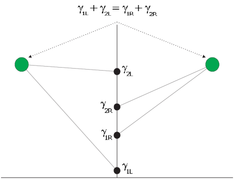
Figure 4: Weight diagram, Case 1: no degeneration

1. $\gamma_{1L}<\gamma_{1R}<\gamma_{2R}<\gamma_{2L}\quad$ (Fig.4)
   The general, physically most interesting case. Every solution yields four waves with pairwise distinct modes.

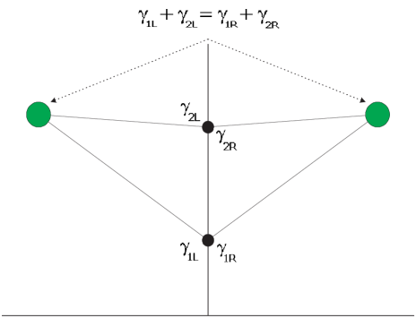
Figure 5: Weight diagram, Case 2: left-right degeneration

2. $\gamma_{1L}=\gamma_{1R}<\gamma_{2R}=\gamma_{2L}\quad$ (Fig.5)
   

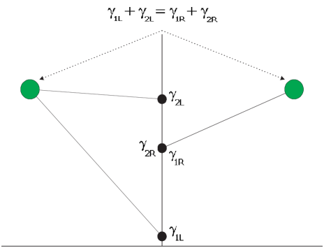
Figure 6: Weight diagram, Case 3: right degeneration

3. $\gamma_{1L}<\gamma_{1R}=\gamma_{2R}<\gamma_{2L}\quad$ (Fig.6)
   

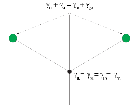
Figure 7: Weight diagram, Case 4: total degeneration

4. $\gamma_{1L}=\gamma_{1R}=\gamma_{2R}=\gamma_{2L}\quad$ (Fig.7)
   The ”most degenerate” case.

The search is organized as follows. Each admissible sum of weights $S_{\gamma};\quad 2\leq S_{\gamma}\leq Mul(q)$ is partitioned into sum of two numbers $S_{\gamma}=\gamma_{1L}+\gamma_{2L},\quad 1\leq\gamma_{1L}\leq\gamma_{2L}\leq Mul(q)$. Then the same number is partitioned into sum of $\gamma_{1R},\gamma_{2R},\quad\gamma_{1L}\leq\gamma_{1R}\leq\gamma_{2R}\leq\gamma_{2L}$. Evidently, if $S_{\gamma}\leq Mul(q)+1$ then the minimal $\gamma_{1L}$ is $1$, otherwise it is $S_{\gamma}-Mul(q)$ (to provide $\gamma_{1R}\leq Mul(q)$). The maximal $\gamma_{1L}$ is always $\lfloor S_{\gamma}/2\rfloor$ and similarly $\gamma_{1R}\leq\lfloor S_{\gamma}/2\rfloor$.

The computational complexity of this step can be estimated as $T=O(Mul(q)^{3})$ due to $O(Mul(q))$ possibilities for each of three values $S_{\gamma},\gamma_{1L},\gamma_{1R}$. As $Mul(q)=\lfloor(2D^{2}/q)^{1/4}\rfloor$, $\quad T=O((2D^{2}/q)^{3/4})$.

Remark.

This step contains an evident redundancy. Indeed, the equation 14 need not be solved independently for each class. Instead, its solutions for all $S_{\gamma}$ could be computed in advance and stored in a look-up table. However, this involves significant computational overhead (e.g. the lookup procedure includes computing the minimal $\gamma_{1L}=max(1,S_{\gamma}-Mul(q))$, which must be done for each class) wiping out the gains of this approach, at least for our basic domain $D=10^{3}$. Nevertheless, this approach should be kept in view if need for computations in much larger domains, say $D=10^{6}$, arises.

Remark.

The general case is not really so general - most classes have small multiplicities and then degenerate cases prevail. The overall distribution is given below:

$Case$	$1$	$2$	$3$	$4$
$Classes$	24368	57666	13987	63778

3.3.4 Step 4. Discarding ”Lean” Classes

In the main domain $D\leq 10^{3}$ we encounter 384145 classes. This sounds like a lot - however, most of these can be processed without computations or with very simple computations. Notice the simple fact that if a class has multiplicity $1$, Sys.(8) takes the form

$$\begin{cases}q=m_{1L}^{2}+n_{1L}^{2}=m_{2L}^{2}+n_{2L}^{2}=m_{1R}^{2}+n_{1R}^{2}=m_{2R}^{2}+n_{2R}^{2}\\ m_{1L}+m_{2L}=m_{1R}+m_{2R}\\ n_{1L}+n_{2L}=n_{1R}+n_{2R}\\ \end{cases}$$ (16)

and for any nontrivial solution the four vectors $(m_{i},n_{i})$ should be pairwise distinct. In terms of the weight equation of the previous section it means that solutions, if any, have to belong to the fourth (”most degenerate”) case. It is evident that no solution of Sys.(16) with pairwise distinct $(m_{i},n_{i})$ exist for $q$ having few decompositions into sum of two squares: one ($q=m^{2}+m^{2}$), two ($q=m^{2}+n^{2}=n^{2}+m^{2}$) and three ($q=m^{2}+n^{2}=n^{2}+m^{2}=l^{2}+l^{2}$). It can be shown by means of elementary algebra that this also holds for $q$ having four decompositions.

Remark.

It is very probable that for classes of multiplicity 1 no nontrivial solutions exist, whatever the number of decompositions into sum of two squares. The question is presently under study. In the main domain $D=10^{3}$ we encounter 357183 classes of multiplicity $1$ (1-classes). This is about $93\%$ of all classes in the domain. Among them, the number of decompositions into sum of two squares is distributed as follows:

$Dec(q)$	$0$	$1$	$2$	$3$	$4$	$5$	$6$	$7$	$8$
$Classes$	110562	256	138044	163	78886	3	8727	2	16595

$Dec(q)$	$14$	$16$	$18$	$20$	$24$	$26$	$32$	$9$	$10$	$12$
$Classes$	38	1015	84	1	75	1	1	31	269	2429

Table 1. Distribution of decomposition number $Mul(q)$ for 1-classes $q$ in the main domain $D=1000$

It follows that 327911 1-classes can be discarded without any computations at all and only 29272 must be checked for probable solutions.

3.3.5 Step 5. Checking Linear Conditions: Symmetries and Signs

Sum-of-weights equation solved and decompositions into sum of two squares found, we need only check the linear conditions to find all solutions. On the face of it, the step is trivial, however some underwater obstacles have to be taken into account. Having found a four-tuple of vectors $(m_{i},n_{i})$ satisfying the first equation of Sys.(8) with both coordinates non-negative, solutions of the system will be found taking all combinations of signs satisfying

$$\begin{cases}\pm m_{1}\pm m_{2}=\pm m_{3}\pm m_{4}\\ \pm n_{1}\pm n_{2}=\pm n_{3}\pm n_{4}\\ \end{cases}$$ (17)

Even the straightforward approach does not need more than $2^{8}$ comparisons, so this step does not consume very much computing time. However, a few points may not be overlooked in order to organize correct, exhaustive and efficient search:

• For the system to represent a four-wave interaction, all the four waves must be pairwise unequal. For the first degenerate case of the weight diagram (Fig.5) we must provide $m_{1L}\neq m_{1R}$ and $m_{2R}\neq m_{2R}$. For the second one (Fig.6) - $m_{1R}\neq m_{2R}$ and for total degeneration (Fig.7) - $m_{1L}\neq m_{2L}\neq m_{1R}\neq m_{2R}$.

• One and the same solution may not occur among the 256 sign combinations twice. First, this could happen due to some $m_{i}$ or $n_{i}$ being $0$ (evidently, the $\pm$ variation should not be done for any $0$ coordinate). Next, sign variation could lead to a transposition of wave vectors. For example, for $q=1$ and $\gamma_{1}+\gamma_{2}=10$ we obtain solutions

  $$\begin{cases}(0,-9)(0,49)\ \Rightarrow\ (15,20)(-15,20)\\ \mbox{and}\\ (0,-9)(0,49)\ \Rightarrow\ (-15,20)(15,20)\\ \end{cases}$$

  which really represent one and the same four-tuple.

• The set of solutions possesses some evident symmetries: if

  $$(m_{1L},n_{1L})(m_{2L},m_{2L})\ \Rightarrow\ (m_{1R},n_{1R})(m_{2R},m_{2R})$$

  then, of course,

  $$(-m_{1L},n_{1L})(-m_{2L},n_{2L})\ \Rightarrow\ (-m_{1R},n_{1R})(-m_{2R},n_{2R})$$

  $$(m_{1L},-n_{1L})(m_{2L},-n_{2L})\ \Rightarrow\ (m_{1R},-n_{1R})(m_{2R},-n_{2R})$$

  $$(-m_{1L},-n_{1L})(-m_{2L},-n_{2L})\ \Rightarrow\ (-m_{1R},-n_{1R})(-m_{2R},-n_{2R})$$

Taking into account these points, an effective search is constructed easily.

4 EXAMPLE TWO: PLANETARY WAVES

In this Section we demonstrate the flexibility of our algorithm. Namely, we solve essentially the same problem - finding all integer solutions in a finite domain $-D\leq m,n\leq D$ for three-wave interactions and another wave type (the so-called ”planetary waves”). In this case $c=-2$ and the main equation, corresponding to (8), has the form

$$\begin{cases}\frac{1}{\sqrt{m_{1}^{2}+n_{1}^{2}}}+\frac{1}{\sqrt{m_{2}^{2}+n_{2}^{2}}}=\frac{1}{\sqrt{m_{3}^{2}+n_{3}^{2}}}\\ m_{1}+m_{2}=m_{3}\end{cases}$$ (18)

where $|m_{i}|,|n_{i}|\leq D$.

4.1 Steps that Stay

• Step 1 - sieving out possible class bases - undergoes minimal changes. For $c=-2$, each $q$ should be a square-free number and not divisible by any prime $p=4u+3$. Evidently, for this wave type the set of class indices is a subset of class indices of the previous section.

• Step 2 - decomposition into two squares - can be preserved one-to-one. Indeed, there are sophisticated algorithms for representing square-free numbers as sums of two squares that are slightly more efficient than in the general case (one used in the previous section) but this step is not the bottleneck of the algorithm.

4.2 Steps to be Modified

• Step 3 - the weight equation is in this case

  $$\frac{1}{\gamma_{1}}+\frac{1}{\gamma_{2}}=\frac{1}{\gamma_{3}}$$ (19)

  or

  $$\gamma_{3}=\frac{\gamma_{1}\gamma_{2}}{\gamma_{1}+\gamma_{2}}$$ (20)

  which has relatively few solutions in integers. Indeed, even for class $1$ with multiplicity $1414$ we obtain only $3945$ solutions.

  Remark.

  For this example it makes sense to generate and store the set of triads $(\gamma_{1},\gamma_{2},\gamma_{3})$ which constitute integer solutions of the Eq.(19) for $1\leq\gamma_{i}\leq Mul(1)$ and for each class $q$ just take its subset $1\leq\gamma_{i}\leq Mul(q)$.

• Step 4 - discarding ”lean” classes - becomes trivial: no class with multiplicity $1$ yields an integer solution of 19. We need only consider $63828$ classes ($q_{63828}=499993,\quad q_{63829}=500009$) from $243143$ in the main domain.

• Step 5 - checking linear conditions - is also much easier than in the previous example, i.e. one equation with three variables instead of two equations with four variables each.

5 DISCUSSION

Our algorithm has been implemented in VBA programming language; computation time (without disk output of solutions found) on a low-end PC (800 MHz Pentium III, 512 MB RAM) is about 4.5 minutes for Example 1 and 1.5 minutes for Example 2. Some overall numerical data for both examples is given in the Tables and Figures below:

$Domain$	$\leq 200$	$\leq 400$	$\leq 600$	$\leq 800$	$\leq 1000$
$Solutions$	263648	800435	932475	1127375	1389657

Table 2. Example 1: Distribution of the number of solutions depending on the chosen main domain $D$.

It is interesting that though the overall number of solutions grows sublinearly as we extend the domain, the number of asymmetrical solutions ($\gamma_{1}\neq\gamma_{2}\neq\gamma_{3}\neq\gamma_{4}$), physically most important ones, grows faster than linearly:

$Domain$	$\leq 200$	$\leq 400$	$\leq 600$	$\leq 800$	$\leq 1000$
$Solutions$	96	344	744	1328	2088

Table 3. Example 1: Distribution of the number of the asymmetrical solutions depending on the chosen main domain $D$.

Notice that considerable part of them (185 of the overall 2088) lie outside of the $D=950$ area, e.g.:

$$(-150,-25)(990,945)\ \Rightarrow\ (294,49)(546,871)$$

$$\mbox{where}\quad q=37,\quad\gamma_{1}=5,\quad\gamma_{2}=15,\quad\gamma_{3}=7,\quad\gamma_{4}=13,$$

$$(128,256)(990,180)\ \Rightarrow\ (400,200)(718,236)$$

$$\mbox{where}\quad q=20,\quad\gamma_{1}=8,\quad\gamma_{2}=15,\quad\gamma_{3}=10,\quad\gamma_{4}=13,$$

$$(-80,-76)(980,931)\ \Rightarrow\ (180,171)(720,684)$$

$$\mbox{where}\quad q=761,\quad\gamma_{1}=2,\quad\gamma_{2}=7,\quad\gamma_{3}=3,\quad\gamma_{4}=6$$

etc. As a whole, asymmetrical solutions are distributed not uniformly along the wave spectrum but are rather grouped around some specific wave numbers. For instance, the first group of asymmetrical solutions (containing 8 solutions) appears in the domain $D=50$, with solution

$$(-4,-4)(49,49)\ \Rightarrow\ (9,9)(36,36),$$

and others, while in the domains $D=60,70,80,90$ there are no new asymmetrical solutions. The next new group (16 solutions) appears in the domain $D=100$, and so on. From the physical point of view, asymmetrical solutions are the most interesting ones because they generate new wave lengths and, therefore, distribute energy through the scales. As it was pointed out quite recently [12], asymmetrical solutions play an extremely important role in wave turbulence. Indeed, no profound understanding of turbulence can be achieved without studying properties which is in our agenda.

Numerical data for the case of planetary waves are given in the Table 4 below:

$Domain$	$\leq 200$	$\leq 400$	$\leq 600$	$\leq 800$	$\leq 1000$
$Solutions$	1099	3137	5664	8565	11795

Table 4. Example 2: Distribution of the number of solutions depending on the chosen main domain $D$.

This data is presented graphically in Figs. 8-11. Number of asymmetric solutions for Example 1 (gravity waves) and total solutions for Example 2 (planetary waves) show smooth power growth and probably are asymptotically power functions of the domain size $D$. On the contrary, the total solution number for Example 1 has an unexpected twist about $D=350$ (Fig.8, shown in detail at Fig.9). This phenomenon is presently under study.

Notice that the algorithm presented here allows to find all solutions for wave vectors belonging to the same class. For three-wave interactions of arbitrary wave types this is always the case. For $n$-wave interactions with $n>3$, however, interacting waves may belong to $\lfloor\frac{n}{2}\rfloor$ different classes [13]. Consider for example the four-wave system

$$\begin{cases}\sqrt{k_{1}}+\sqrt{k_{2}}=\sqrt{k_{3}}+\sqrt{k_{4}}\\ \vec{k}_{1}+\vec{k}_{2}=\vec{k}_{3}+\vec{k}_{4}\\ \end{cases}$$

where $k_{1}$ and $k_{3}$ belong to one class and $k_{2}$ and $k_{4}$ - to another one, i.e. the first equation breaks up into two independent equations

$$\sqrt{k_{1}}=\sqrt{k_{3}}\quad\mbox{and}\quad\sqrt{k_{2}}=\sqrt{k_{4}}.$$

In this case, a modified form of our generic algorithm can be applied. This will be dealt with in our next paper.

Acknowledgement. E.K. acknowledges the support of the Austrian Science Foundation (FWF) under projects SFB F013/F1304.

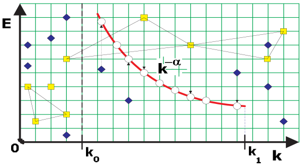
Figure 3: Laminated Wave Turbulence Theory, arbitrary $|\vec{k}|$: Discrete and statistical layers of turbulence co-exist in many wave systems. ZK-energy spectrum contains ”holes” in the nodes of the integer lattice which are depicted by empty circles.

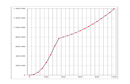
Figure 8: Number of solutions in partial domains

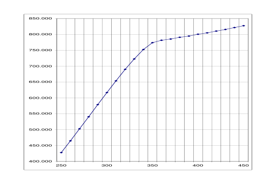
Figure 9: Twist range of Fig. 8 zoomed

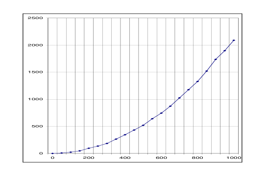
Figure 10: Number of asymmetric solutions in partial domains

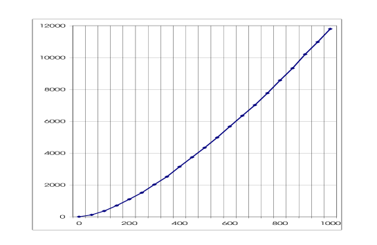
Figure 11: Example 2: Number of solutions in partial domains

References

- [1] A.N. Kolmogorov. The local structure of turbulence in incompressible viscous fluids at very large Reynolds numbers. Dokl. Akad. Nauk SSSR (30), 301-305 (1941). Reprinted: Proc. R. Soc. Lond. A (434), 9-13 (1991)
- [2] V.E.Zakharov, V.S.L’vov, G. Falkovich, Kolmogorov Spectra of Turbulence. (Series in Nonlinear Dynamics, Springer, 1992)
- [3] V.E.Zakharov, N.N. Filonenko. Weak turbulence of capillary waves. J. Appl. Mech. Tech. Phys. (4), 500-515 (1967)
- [4] E.A. Kartashova. Partitioning of ensembles of weakly interacting dispersing waves in resonators into disjoint classes. Physica D (46), 43 (1990); E.A. Kartashova. On properties of weakly nonlinear wave interactions in resonators. Physica D (54), 125 (1991); E.A. Kartashova. Weakly nonlinear theory of finite-size effects in resonators. Phys. Rev. Let. (72), 2013 (1994); E.A. Kartashova. Clipping – a new investigation method for PDE-s in compact domains. Theor. Math. Phys. (99), 675 (1994); E.A. Kartashova. Wave resonances in systems with discrete spectra. AMS Transl. (182), 2, 95 (1998) and others
- [5] E.A. Kartashova. A model of laminated turbulence. JETP Letters (83) 7, 341 (2006)
- [6] E. Kartashova. Fast Computation Algorithm for Discrete Resonances among Gravity Waves. J. Low Temp. Phys. (to appear). E-print arXiv.org:math-ph/0605067 (2006)
- [7] E.A. Kartashova. Wave resonances in systems with discrete spectra. AMS Transl. (182), 2, 95 (1998)
- [8] I. Besikovitch. J. London Math. Society 15, 3 (1940)
- [9] J.M. Basilla Proc. Japan. Acad. 80, Ser. A, 40 (2004)
- [10] H. Cohen, A Course in Computation Number Theory. (Grad. Texts in Math. 138. Springer-Verlag, New York, 1993) 34
- [11] N.P.Prudnikov et.al., Integrals and Rows. Vol. I (Nauka, Moscow, 1981) (in Russian)
-
[12]
Y.V. Lvov, S. Nazarenko, B. Pokorni. Discreteness and its
effect on water-wave turbulence. Physica D (218) 24-35 (2006)
- [13] E.A. Kartashova. Resonant interactions of the water waves with discrete spectra. Proc. of Int. Nonlinear Water Waves Workshop (NWWW), pp.43-53. University of Bristol, England October, 1991