Singular perturbation of quantum stochastic differential equations with coupling through an oscillator mode

Abstract.

We consider a physical system which is coupled indirectly to a Markovian resevoir through an oscillator mode. This is the case, for example, in the usual model of an atomic sample in a leaky optical cavity which is ubiquitous in quantum optics. In the strong coupling limit the oscillator can be eliminated entirely from the model, leaving an effective direct coupling between the system and the resevoir. Here we provide a mathematically rigorous treatment of this limit as a weak limit of the time evolution and observables on a suitably chosen exponential domain in Fock space. The resulting effective model may contain emission and absorption as well as scattering interactions.

1. Introduction

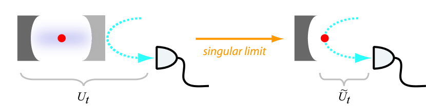
Figure 1. Cartoon illustration of a prototypical problem that falls within the framework of this paper. An atom is placed in a single-mode optical cavity. One of the cavity mirrors is leaky, thus coupling the cavity mode to the external field (which may ultimately be detected). In the “bad cavity” limit the mirror is made so transmissive that the cavity can be eliminated from the description of the model, leaving an effective direct interaction between the atom and the field.

The motivation for this article stems from the following problem in quantum optics, illustrated in Fig. 1. Consider the canonical starting point of cavity QED, an atomic system in an optical cavity. In many cases such a system is well modelled using only a single cavity mode. The cavity is then effectively described by a single quantum harmonic oscillator, and the atom-cavity interaction Hamiltonian takes the form

(1.1) $$H=E_{11}b^{{\dagger}}b+E_{10}b^{{\dagger}}+E_{01}b+E_{00},$$

where $E_{ij}$ are operators acting on the atomic Hilbert space, $E_{ij}^{\dagger}=E_{ji}$, and $b$, $b^{\dagger}$ are the cavity mode annihilation and creation operators, respectively. Usually one of the cavity mirrors is assumed to be perfectly reflective, while the other mirror allows some light to leak into the electromagnetic field outside the cavity and vice versa. In the Markov approximation [1, 2], the time evolution of the entire system (consisting of the atom, cavity and external field) is described by the unitary solution to the Hudson-Parthasarathy [16] quantum stochastic differential equation

(1.2) $$dU_{t}=\left\{\sqrt{\gamma}\,b\,dA_{t}^{\dagger}-\sqrt{\gamma}\,b^{\dagger}\,dA_{t}-\frac{\gamma}{2}\,b^{\dagger}b\,dt-iH\,dt\right\}U_{t},$$

where $A_{t}$, $A_{t}^{\dagger}$ are the usual creation and annihilation processes in the external field. The transmissivity of the leaky mirror is controlled by the positive constant $\gamma$.

In many situations of practical interest, $\gamma$ will be quite large compared to the strengths $\|E_{ij}\|$ of the atom-cavity interaction. When this is the case, one would expect that the presence of the cavity has little qualitative influence on the atomic dynamics: the cavity is then essentially transparent in the frequency range corresponding to the atomic dynamics, so that the atoms “see” the external field directly. Similarly, we expect that measurements obtained from detection of the outgoing field (e.g., by homodyne detection) would depend directly on the atomic observables and would be essentially independent of the cavity observables. The hope is, then, that the time evolution $U_{t}$ can be described in some idealized limit by the unitary solution $\tilde{U}_{t}$ of a new Hudson-Parthasarathy equation which involves only atomic operators and the external field, and in which the cavity has been eliminated. The goal of this article is to make these ideas precise.

Previous work. The elimination of a leaky cavity in the bad cavity limit is an extremely common procedure in the physics literature—so common, in fact, that most papers state the resulting expression without further comment (“we adiabatically eliminate the cavity, giving $\ldots$”). Often the equation considered is a Lindblad-type master equation for the atom and cavity; in our context, this (deterministic) differential equation for the reduced density operator can be obtained by averaging over the field as in [16]. One method that is used to eliminate the cavity in such an equation, see e.g. [26], involves expanding the density operator in matrix elements, setting certain time derivatives to zero, then solving algebraically to obtain an equation for the atomic matrix elements only. This method is commonly known as adiabatic elimination. Though such an approach is not very rigorous, similar techniques can sometimes be justified in the context of the classical theory of singular perturbations (Tikhonov’s theorem [23]). A somewhat different approach, see e.g. [11], uses projection operators and Laplace transform techniques. None of these techniques are applicable to the question posed here, however, as we wish to retain the external field in the limiting model. Hence we are seeking a singular perturbation result for quantum stochastic differential equations, which is (to our knowledge) not yet available in the literature.

A naive attempt at adiabatic elimination for quantum stochastic equations is made in [7] (see also [8, 27]). These authors use the following procedure:

• First, they obtain Heisenberg equations of motion (in Itô form) for the cavity annihilator $b_{t}=U_{t}^{\dagger}bU_{t}$ and also for the relevant atomic operators.

• Next, they set $\dot{b}_{t}=0$ (where the right-hand side is interpreted as “quantum white noise”) and solve algebraically for $b_{t}$.

• Next, they plug this expression into the atomic equations of motion.

• Finally, they interpret these equations as “implicit” equations [25] (a formal analog of Stratonovich equations) and convert to the “explicit form” (a formal analog of Itô equations). The latter are considered to be the adiabatically eliminated Heisenberg equations of motion for the atomic operators.

Attempts at justifying this procedure run into a number of seemingly fatal problems. Forgoing the issue of the mathematical well-posedness of “quantum white noise”, the approximation $\dot{b}_{t}=0$ seems incompatible with the fact that the right-hand side is formally infinite. Next we have to deal with the interpretation of the resulting equations; even in the classical stochastic case, it is known that adiabatically eliminated expressions need not be of Stratonovich type (see [10] for some counterexamples); the singular limit is rather delicate and the resulting outcome depends on the way in which the limit is taken. Ignoring even this issue, it should be pointed out that the implicit-explicit formalism introduced in [25] (essentially along the lines of McShane’s canonical extension [18, 17]) does not even capture correctly the ordinary Markov limit in the presence of scattering interactions; compare the expressions in [25] to the rigorous results obtained in [14]. It is thus highly remarkable (if not miraculous!) that we can essentially reproduce the result of [7] using the methods developed in this paper (see example 4.4 in section 4).

Statement of the problem. Following [10], we seek a “method by which fast variables may be eliminated from the equations of motion in some well-defined limit.” Which limit to take is not entirely obvious at the outset; for example, the naive choice $\gamma\to\infty$ only yields trivial results (the cavity is forced to its ground state and the atomic dynamics vanishes). To define a nontrivial limit, we introduce the scaling parameter $\varepsilon>0$ and make the substitution $b\mapsto\varepsilon^{-1/2}b$ in (1.1) and (1.2). The limit $\varepsilon\to 0^{+}$ then has the character of a central limit theorem, and provides a nontrivial result in which the cavity is eliminated. (Note that similar scaling limits are used in projection operator techniques for master equations [11].)

Our approach, then, is to proceed as follows. First we make the above substitution. Next we switch to the interaction picture with respect to the cavity-field interaction. This gives rise to an interaction picture time evolution in which the atom is driven by a quantum Ornstein-Uhlenbeck process. The limit $\varepsilon\to 0^{+}$ corresponds essentially to a Markov limit of this equation, and consequently our proofs borrow heavily from the methods developed to treat such limits (particularly from the estimates developed in [14]). However, our limits are of a somewhat stronger character than those considered in [1, 2, 14] as we take weak limits on a fixed domain in the underlying Hilbert space, rather than “limits in matrix elements” where the domain depends on $\varepsilon$. We also consider, aside from the time evolution unitary and the Heisenberg evolution of the atomic observables, the limiting behavior of the output field operators (which can be observed e.g. through homodyne detection).

For concreteness, we will restrict ourselves to the model described by (1.1) and (1.2). This model is already very rich and widely used in the literature in various scenarios. Our results can also be extended to more complicated setups, in particular to the case of multiple external fields and oscillators along the lines of [15]; the subsequent extension to thermal and squeezed noises is then also straightforward through the usual double Fock space construction, see e.g. [13], at least in the absence of scattering interactions ($E_{11}=0$).

2. Preliminaries

Throughout this article we work on the product Hilbert space $\mathfrak{h}=\mathfrak{h}_{\mathrm{sys}}\otimes\mathfrak{h}_{\mathrm{osc}}\otimes\mathfrak{h}_{\mathrm{resv}}$ consisting of a physical (e.g. atomic) system $\mathfrak{h}_{\mathrm{sys}}$, a quantum harmonic oscillator $\mathfrak{h}_{\mathrm{osc}}=\Gamma(\mathbb{C})$ (describing e.g. a cavity mode), and an external Bosonic resevoir $\mathfrak{h}_{\mathrm{resv}}=\Gamma(L^{2}(\mathbb{R}_{+}))$ (describing e.g. the electromagnetic field). Here $\Gamma(\mathfrak{h}^{\prime})$ denotes the symmetric (Boson) Fock space over the one-particle Hilbert space $\mathfrak{h}^{\prime}$. We use the following notation for Fock space vectors: $|0\rangle\in\Gamma(\mathfrak{h}^{\prime})$ denotes the vacuum vector, $|f\rangle\in\Gamma(\mathfrak{h}^{\prime})$ denotes the exponential vector corresponding to $f\in\mathfrak{h}^{\prime}$, and $\mathcal{E}\subset\Gamma(\mathfrak{h}^{\prime})$ denotes the linear space generated by the exponential vectors (the exponential domain). We will also use the subscripts $|f\rangle_{\rm osc}$ or $|f\rangle_{\rm resv}$, and similarly $\mathcal{E}_{\rm osc}$, $\mathcal{E}_{\rm resv}$, wherever confusion may arise.

We define the following standard operators: $b$ and $b^{\dagger}$ are the creation and annihilation operators on $\mathfrak{h}_{\mathrm{osc}}$, and $A_{t}$, $A_{t}^{\dagger}$ and $\Lambda_{t}$ are the usual annihilation, creation and gauge processes on $\mathfrak{h}_{\mathrm{resv}}$, respectively [16]. We denote the ampliations of these operators to $\mathfrak{h}$ by the same symbols. For any $f\in L^{2}(\mathbb{R}_{+})$ and for any real, bounded $g\in L^{\infty}(\mathbb{R}_{+})\cap L^{2}(\mathbb{R}_{+})$ we also define the field operators [16]

$$A(f)=\int_{0}^{\infty}f(t)^{*}\,dA_{t},\qquad A(f)^{\dagger}=\int_{0}^{\infty}f(t)\,dA_{t}^{\dagger},\qquad\Lambda(g)=\int_{0}^{\infty}g(t)\,d\Lambda_{t}.$$

We recall that the exponential domain $\mathcal{E}_{\rm resv}$ can be extended to $\mathcal{E}_{\rm resv}^{\prime}\supset\mathcal{E}_{\rm resv}$ in such a way that $\mathcal{E}_{\rm resv}^{\prime}$ is invariant under the action of $A(f)$, $A(f)^{\dagger}$ and $\Lambda(g)$, see e.g. [19, pp. 61–65]. Similarly $\mathcal{E}_{\rm osc}$ can be extended to $\mathcal{E}_{\rm osc}^{\prime}$ so that the latter is invariant under $b$, $b^{\dagger}$ and $b^{\dagger}b$. This means in particular that the domain $\mathcal{D}^{\prime}=\mathfrak{h}_{\rm sys}\underline{\otimes}\mathcal{E}_{\rm osc}^{\prime}\underline{\otimes}\mathcal{E}_{\rm resv}^{\prime}\subset\mathfrak{h}$ is invariant under finite linear combinations of operators of the form $E\otimes\{b,b^{\dagger},b^{\dagger}b\}\otimes\{A(f),A(f)^{\dagger},\Lambda(g)\}$, and that commutators of such operators are well defined on $\mathcal{D}^{\prime}$. Here $E$ is any bounded operator on $\mathfrak{h}_{\rm sys}$ and $\underline{\otimes}$ denotes the algebraic tensor product. We recall also the useful identities $|\alpha\rangle_{\rm osc}=\exp(\alpha b^{{\dagger}})|0\rangle_{\rm osc}$ and $|f\rangle_{\mathrm{resv}}=\exp(A(f)^{{\dagger}})|0\rangle_{\mathrm{resv}}$ [20, sec. II.20].

The starting point for our investigation is the rescaled version of (1.1) and (1.2). We consider the unitary solution $U_{t}(\varepsilon)$, given the initial condition $U_{0}(\varepsilon)=I$, to the Hudson-Parthasarathy quantum stochastic differential equation (QSDE)

(2.1) $$dU_{t}(\varepsilon)=\left\{\sqrt{\frac{\gamma}{\varepsilon}}\,b\,dA_{t}^{{\dagger}}-\sqrt{\frac{\gamma}{\varepsilon}}\,b^{{\dagger}}\,dA_{t}-\frac{\gamma}{2\varepsilon}\,b^{{\dagger}}b\,dt-i\,H(\varepsilon)\,dt\right\}U_{t}(\varepsilon),$$

where the Hamiltonian $H(\varepsilon)$ is taken to be of the form

(2.2) $$H(\varepsilon)=\frac{1}{\varepsilon}\,E_{11}b^{{\dagger}}b+\frac{1}{\sqrt{\varepsilon}}\,E_{10}b^{{\dagger}}+\frac{1}{\sqrt{\varepsilon}}\,E_{01}b+E_{00}.$$

Here $E_{ij}$, $\|E_{ij}\|<\infty$ are (the ampliations of) given bounded operators on $\mathfrak{h}_{\rm sys}$, $E_{ij}^{{\dagger}}=E_{ji}$, and $\gamma,\varepsilon>0$ are positive constants. The existence, uniqueness and unitarity of the solution of (2.1) are established in [9].

The interaction picture. We are interested in the limit $\varepsilon\rightarrow 0^{+}$. As the oscillator-resevoir dynamics becomes singular in this limit, the first step we take is to remove these dynamics by going over to the interaction representation. To this end, define the oscillator-resevoir time evolution $V_{t}(\varepsilon)$ as the unitary solution of

$$dV_{t}(\varepsilon)=\left\{\sqrt{\frac{\gamma}{\varepsilon}}\,b\,dA_{t}^{{\dagger}}-\sqrt{\frac{\gamma}{\varepsilon}}\,b^{{\dagger}}\,dA_{t}-\frac{\gamma}{2\varepsilon}\,b^{{\dagger}}b\,dt\right\}V_{t}(\varepsilon),$$

where $V_{0}(\varepsilon)=I$. Existence, uniqueness and unitarity are again guaranteed by [9]. We wish to consider the unitary

(2.3) $$\tilde{U}_{t}(\varepsilon)=V_{t}(\varepsilon)^{\dagger}U_{t}(\varepsilon).$$

Using the quantum Itô rules [16], we find that $\tilde{U}_{t}(\varepsilon)$ is given by the solution of the Schrödinger equation

(2.4) $$\frac{d\tilde{U}_{t}(\varepsilon)}{dt}=-i\,\tilde{\Upsilon}_{t}(\varepsilon)\tilde{U}_{t}(\varepsilon),\qquad\tilde{U}_{0}(\varepsilon)=I,$$

with time-dependent interaction Hamiltonian

(2.5) $$\tilde{\Upsilon}_{t}(\varepsilon)=V_{t}(\varepsilon)^{{\dagger}}H(\varepsilon)V_{t}(\varepsilon).$$

Note that $V_{t}(\varepsilon)$ commutes with any system operator $E$ (on $\mathfrak{h}_{\rm sys})$, so we have $E_{t}(\varepsilon)=U_{t}(\varepsilon)^{\dagger}EU_{t}(\varepsilon)=\tilde{U}_{t}(\varepsilon)^{\dagger}E\tilde{U}_{t}(\varepsilon)$. Hence in order to study limits of the form $\lim_{\varepsilon\to 0^{+}}E_{t}(\varepsilon)$ it is sufficient to consider $\tilde{U}_{t}(\varepsilon)$ rather than $U_{t}(\varepsilon)$.

Quantum Ornstein-Uhlenbeck processes. It is convenient to introduce the quantum Ornstein-Uhlenbeck (O-U) annihilation and creation processes

(2.6) $$\tilde{a}_{t}(\varepsilon)=-\sqrt{\frac{\gamma}{4\varepsilon}}\,V_{t}(\varepsilon)^{{\dagger}}bV_{t}(\varepsilon),\qquad\tilde{a}_{t}(\varepsilon)^{\dagger}=-\sqrt{\frac{\gamma}{4\varepsilon}}\,V_{t}(\varepsilon)^{{\dagger}}b^{\dagger}V_{t}(\varepsilon).$$

Using the quantum Itô rules, we find that

$$d\tilde{a}_{t}(\varepsilon)=\frac{\gamma}{2\varepsilon}\,dA_{t}-\frac{\gamma}{2\varepsilon}\,\tilde{a}_{t}(\varepsilon)\,dt,\qquad\tilde{a}_{0}(\varepsilon)=-\sqrt{\frac{\gamma}{4\varepsilon}}\,b.$$

Solving explicitly, we obtain

(2.7) $$\tilde{a}_{t}(\varepsilon)=\sqrt{\frac{\gamma}{4\varepsilon}}\,e^{-\gamma t/2\varepsilon}\left[\sqrt{\frac{\gamma}{\varepsilon}}\int_{0}^{t}e^{\gamma u/2\varepsilon}\,dA_{u}-b\right].$$

This allows us to express the interaction Hamiltonian $\tilde{\Upsilon}_{t}(\varepsilon)$ in the form

(2.8) $$\tilde{\Upsilon}_{t}(\varepsilon)=\frac{4}{\gamma}\,E_{11}\tilde{a}_{t}(\varepsilon)^{\dagger}\tilde{a}_{t}(\varepsilon)-\frac{2}{\sqrt{\gamma}}\,E_{10}\tilde{a}_{t}(\varepsilon)^{\dagger}-\frac{2}{\sqrt{\gamma}}\,E_{01}\tilde{a}_{t}(\varepsilon)+E_{00}.$$

Lemma 2.1.

The O-U processes satisfy (on $\mathcal{D}^{\prime}$) the commutation relations

(2.9) $$[\tilde{a}_{t}(\varepsilon),\tilde{a}_{s}(\varepsilon)]=0,\qquad[\tilde{a}_{t}(\varepsilon),\tilde{a}_{s}(\varepsilon)^{\dagger}]=G_{\varepsilon}(t-s),$$

where the correlation function $G_{\varepsilon}(\tau)$ is given by

$$G_{\varepsilon}(\tau)=\frac{\gamma}{4\varepsilon}\,\exp\left(-\frac{\gamma|\tau|}{2\varepsilon}\right).$$

Proof.

Recall [20, sec. II.20] the commutation relation on $\mathcal{D}^{\prime}$

$$[A(f),A(g)^{\dagger}]=\int_{0}^{\infty}f(t)^{*}g(t)\,dt.$$

Hence we obtain

$$\left[e^{-\gamma t/2\varepsilon}\int_{0}^{t}e^{\gamma u/2\varepsilon}\,dA_{u},e^{-\gamma s/2\varepsilon}\int_{0}^{s}e^{\gamma u/2\varepsilon}\,dA_{u}^{\dagger}\right]=\\ e^{-\gamma(t+s)/2\varepsilon}\int_{0}^{t\wedge s}e^{\gamma u/\varepsilon}\,du=\frac{\varepsilon}{\gamma}\,e^{-\gamma(t+s-2\,t\wedge s)/2\varepsilon}-\frac{\varepsilon}{\gamma}\,e^{-\gamma(t+s)/2\varepsilon},$$

where $t\wedge s=\min(t,s)$. Now note that $t+s-2\,t\wedge s=|t-s|$. Hence writing out the full commutators and using $[b,b^{\dagger}]=1$, the result follows. ∎

The function $G_{\varepsilon}(\cdot)$ has the property of being strictly positive, symmetric and integrable with $\int_{-\infty}^{\infty}G_{\varepsilon}(\tau)\,d\tau=1$. In the limit $\varepsilon\to 0^{+}$, $G_{\varepsilon}(\cdot)$ therefore converges in the sense of distributions to a delta function at the origin. This means that the Ornstein-Uhlenbeck processes $\tilde{a}_{t}(\varepsilon)$, $\tilde{a}_{t}(\varepsilon)^{\dagger}$ formally converge to quantum white noises as $\varepsilon\to 0^{+}$. Let us remark that these processes may now be written as

(2.10) $$\tilde{a}_{t}(\varepsilon)=2\int_{0}^{t}G_{\varepsilon}(t-s)\,dA_{s}-\sqrt{\frac{4\varepsilon}{\gamma}}\,G_{\varepsilon}(t)\,b.$$

3. Strong coupling limit ($\varepsilon\to 0^{+}$)

For any $g\in L^{2}(\mathbb{R}_{+})$ we define the future and past smoothed functions

$$g^{+}(t,\varepsilon) = 2\int_{0}^{\infty}g(t+\tau)G_{\varepsilon}(\tau)\,d\tau=2\int_{t}^{\infty}g(\tau)G_{\varepsilon}(t-\tau)\,d\tau,$$

$$g^{-}(t,\varepsilon) = 2\int_{0}^{t}g(t-\tau)G_{\varepsilon}(\tau)\,d\tau=2\int_{0}^{t}g(\tau)G_{\varepsilon}(t-\tau)\,d\tau.$$

We will encounter such functions repeatedly in the following. If $g$ were a continuous function, we would have the limits

(3.1) $$\lim_{\varepsilon\to 0^{+}}g^{\pm}(t,\varepsilon)=g(t).$$

The space $L^{2}(\mathbb{R}_{+})$ is much too large, however, to ensure that the $\varepsilon\to 0^{+}$ limits of the smoothed functions are well behaved; consider for example a square integrable function with oscillatory discontinuity (e.g. $\sin(1/x)$). To avoid such unpleasantness we will restrict our attention to the set of regulated square integrable functions, following [12].

Definition 3.1.

Let $L^{2}_{\pm}(\mathbb{R}_{+})\subset L^{2}(\mathbb{R}_{+})\cap L^{\infty}(\mathbb{R}_{+})$ denote the set of square integrable bounded functions $f$ on the halfline such that the limits $f(t^{\pm})=\lim_{s\to t^{\pm}}f(s)$ exist at every point $t\in\mathbb{R}_{+}$. We denote by $\mathcal{E}^{\pm}_{\rm resv}\subset\mathcal{E}_{\rm resv}$ the restricted exponential domain generated by exponential vectors with amplitude functions in $L^{2}_{\pm}(\mathbb{R}_{+})$.

Before moving on, we make the following remarks:

1. Any $g\in L^{2}_{\pm}(\mathbb{R}_{+})$ has at most a countable number of discontinuity points (see e.g. [5, chapter 3]). Hence for such $g$ Eq. (3.1) holds for (Lebesgue-)a.e. $t\in\mathbb{R}_{+}$.

2. Note that if $g\in L^{2}_{\pm}(\mathbb{R}_{+})$, then $\chi_{[0,s]}g\in L^{2}_{\pm}(\mathbb{R}_{+})$ for any $s\in\mathbb{R}_{+}$. Hence $\mathcal{E}^{\pm}_{\rm resv}$ is a suitable choice for the restricted exponential domain used in the construction of the Hudson-Parthasarathy stochastic integration theory [16].

For future reference, we collect various $\varepsilon\to 0^{+}$ limits in the following lemma.

Lemma 3.2.

For any $g\in L^{2}_{\pm}(\mathbb{R}_{+})$, the following hold: $g^{\pm}(t,\varepsilon)\xrightarrow{\varepsilon\to 0^{+}}g(t^{\pm})$,

$$\lim_{\varepsilon\to 0^{+}}\int_{0}^{\infty}G_{\varepsilon}(t-s)g(s)\,ds=\lim_{\varepsilon\to 0^{+}}2\int_{0}^{t}G_{\varepsilon}(t-s)g^{+}(s,\varepsilon)\,ds=\frac{g(t^{+})+g(t^{-})}{2}.$$

Moreover, all these expressions are equal to $g(t)$ for (Lebesgue-)a.e. $t\in\mathbb{R}_{+}$; hence it follows that $g^{\pm}(\cdot,\varepsilon)\xrightarrow[\varepsilon\to 0^{+}]{}g(\cdot)$ in $L^{2}(\mathbb{R}_{+})$, etc.

Proof.

The first statement follows from

$$g^{+}(t,\varepsilon)=\int_{0}^{\infty}\frac{\gamma}{2}\,e^{-\gamma\tau/2}\,g(t+\varepsilon\tau)\,d\tau\xrightarrow{\varepsilon\to 0^{+}}g(t^{+}),$$

where we have used dominated convergence to take the limit. Similarly

$$g^{-}(t,\varepsilon)=\int_{0}^{\infty}\frac{\gamma}{2}\,e^{-\gamma\tau/2}\,g(t-\varepsilon\tau)\chi_{[0,t/\varepsilon]}(\tau)\,d\tau\xrightarrow{\varepsilon\to 0^{+}}g(t^{-}).$$

The third statement follows directly as

$$\int_{0}^{\infty}G_{\varepsilon}(t-s)g(s)\,ds=\frac{g^{+}(t,\varepsilon)+g^{-}(t,\varepsilon)}{2}.$$

To prove the next statement, note that

$$2\int_{0}^{t}G_{\varepsilon}(t-s)g^{+}(s,\varepsilon)\,ds=\int_{0}^{\infty}g(\tau)\left[4\int_{0}^{t\wedge\tau}G_{\varepsilon}(t-s)G_{\varepsilon}(s-\tau)\,ds\right]d\tau.$$

But straightforward calculation yields

$$4\int_{0}^{t\wedge\tau}G_{\varepsilon}(t-s)G_{\varepsilon}(s-\tau)\,ds=G_{\varepsilon}(t-\tau)-G_{\varepsilon}(\tau)\,\exp\left(-\frac{\gamma t}{2\varepsilon}\right),$$

and the result follows directly. Finally, the last statement of the lemma follows from the fact that $g$ has at most a countable number of discontinuities, together with the dominated convergence theorem. ∎

For $f\in L_{\pm}^{2}(\mathbb{R}^{+})$, we define the smeared field operator

(3.2) $$\tilde{A}(f,\varepsilon)=\int_{0}^{\infty}f(t)^{\ast}\tilde{a}_{t}(\varepsilon)\,dt.$$

It is straightforward to obtain the commutation relation

$$[\tilde{A}(f,\varepsilon),\tilde{A}(g,\varepsilon)^{{\dagger}}]=\int_{0}^{\infty}f(t)^{*}G_{\varepsilon}g(t)\,dt=\frac{1}{2}\int_{0}^{\infty}f(t)^{*}(g^{+}(t,\varepsilon)+g^{-}(t,\varepsilon))\,dt,$$

where we have written $G_{\varepsilon}g(t)=\int_{0}^{\infty}G_{\varepsilon}(t-s)g(s)\,ds=\frac{1}{2}g^{+}(t,\varepsilon)+\frac{1}{2}g^{-}(t,\varepsilon)$. Using (2.10), we may also express the smeared field as

(3.3) $$\tilde{A}(f,\varepsilon)=A(f_{\varepsilon}^{+})-\sqrt{\frac{\varepsilon}{\gamma}}\,f^{+}(0,\varepsilon)^{\ast}b,$$

where $f_{\varepsilon}^{+}(t)=f^{+}(t,\varepsilon)$. The second term ought to be negligible in the $\varepsilon\rightarrow 0^{+}$ limit and indeed, if $\varphi\in\mathfrak{h}_{\rm osc}$ is a vector with $\|b\varphi\|<\infty$ and if $e(g)=|g\rangle_{\rm resv}$ is an exponential vector ($g\in L^{2}(\mathbb{R}_{+})$), then

$$\frac{\|(\tilde{A}(f,\varepsilon)-A(f))\,\varphi\otimes e(g)\|}{\|\varphi\otimes e(g)\|}\leq\frac{\|A(f_{\varepsilon}^{+}-f)\,e(g)\|}{\|e(g)\|}+\sqrt{\frac{\varepsilon}{\gamma}}\,f^{+}(0,\varepsilon)^{\ast}\frac{\|b\varphi\|}{\|\varphi\|}\\ =\left|\int_{0}^{\infty}(f^{+}(t,\varepsilon)-f(t))^{*}g(t)\,dt\right|+\sqrt{\frac{\varepsilon}{\gamma}}\,f^{+}(0,\varepsilon)^{\ast}\frac{\|b\varphi\|}{\|\varphi\|}\xrightarrow{\varepsilon\to 0^{+}}0.$$

More generally, we can define the smeared Weyl operators

(3.4) $$\tilde{W}(f,\varepsilon)=\exp\left\{\tilde{A}(f,\varepsilon)^{{\dagger}}-\tilde{A}(f,\varepsilon)\right\},$$

which satisfy the smeared canonical commutation relations

(3.5) $$\tilde{W}(f,\varepsilon)\tilde{W}(g,\varepsilon)=\tilde{W}(f+g,\varepsilon)\,\exp\left\{-i\,\,\mathrm{Im}\int_{0}^{\infty}f(t)^{*}G_{\varepsilon}g(t)\,dt\right\}.$$

The smeared Weyl operator $\tilde{W}(f,\varepsilon)$ ought to converge to the standard Weyl unitary $W(f)=I_{\rm osc}\otimes\exp\{A(f)^{\dagger}-A(f)\}$ as $\varepsilon\to 0^{+}$. It is indeed not difficult to establish that for arbitrary $f_{1},\cdots f_{n}\in L_{\pm}^{2}(\mathbb{R}_{+})$

$$\|(\tilde{W}(f_{1},\varepsilon)\cdots\tilde{W}(f_{n},\varepsilon)-W(f_{1})\cdots W(f_{n}))\,\varphi\otimes e(g)\|\xrightarrow{\varepsilon\to 0^{+}}0.$$

This time, no restriction needs to be placed on $\varphi$. This is a type of quantum central limit theorem, however, it is less abstract than the “limit in matrix elements” traditionally encountered in the quantum probability literature [1, 2, 14] since the limit is taken on the fixed domain $\mathfrak{h}_{\rm osc}\underline{\otimes}\mathcal{E}_{\rm resv}$. The limiting operator is thus defined on the same Hilbert space, though it acts non-trivially on the noise space only.

4. Limit dynamics

The limit of the process $\{\tilde{U}_{t}(\varepsilon):t\geq 0\}$ as $\varepsilon\to 0^{+}$ is reminiscent of the Markov limits that have been widely studied in mathematical physics [1, 2, 14]. Comparison with previous results suggests that the limit be again described by a quantum stochastic process $\{\tilde{U}_{t}:t\geq 0\}$. We wish to deduce this limiting process by studying the limit of matrix elements $\langle\psi_{1}|\tilde{U}_{t}(\varepsilon)\psi_{2}\rangle$ for arbitrary vectors of the form

$$\psi_{i}=v_{i}\otimes|\alpha_{i}\rangle_{\rm osc}\otimes|f_{i}\rangle_{\rm resv},\qquad v_{i}\in\mathfrak{h}_{\rm sys},~{}\alpha_{i}\in\mathbb{C},~{}f_{i}\in L^{2}_{\pm}(\mathbb{R}_{+}).$$

In other words, we would like to obtain $\tilde{U}_{t}$ as the weak limit of $\tilde{U}_{t}(\varepsilon)$, as $\varepsilon\to 0^{+}$, on the domain $\mathfrak{h}_{\rm sys}\underline{\otimes}\mathcal{E}_{\rm osc}\underline{\otimes}\mathcal{E}_{\rm resv}^{\pm}$. We will similarly study weak limits of observables $\tilde{U}_{t}(\varepsilon)^{\dagger}E\tilde{U}_{t}(\varepsilon)$, where $E$ is a system observable, on the same domain.

Formally, we may expand $\tilde{U}_{t}(\varepsilon)$ as a Dyson series (by Picard iteration):

(4.1) $$\tilde{U}_{t}(\varepsilon)=I+\sum_{n=1}^{\infty}(-i)^{n}\int_{\Delta_{n}(t)}ds_{n}\cdots ds_{1}\,\tilde{\Upsilon}_{s_{n}}(\varepsilon)\cdots\tilde{\Upsilon}_{s_{1}}(\varepsilon),$$

where the multi-time integrals are taken over the simplex

$$\Delta_{n}(t)=\{(s_{n},\dots,s_{1}):t>s_{n}>\cdots>s_{1}>0\}.$$

The Dyson series expansion of $\langle\psi_{1}|\tilde{U}_{t}(\varepsilon)\psi_{2}\rangle$ is given by

(4.2) $$\langle\psi_{1}|\psi_{2}\rangle+\sum_{n=1}^{\infty}(-i)^{n}\int_{\Delta_{n}(t)}ds_{n}\cdots ds_{1}\,\langle\psi_{1}|\tilde{\Upsilon}_{s_{n}}(\varepsilon)\cdots\tilde{\Upsilon}_{s_{1}}(\varepsilon)\psi_{2}\rangle.$$

The usual existence proof for differential equations by Picard iteration suggests that the Dyson series are convergent. Following [1, 2, 14], our basic approach will be as follows. First, we obtain an estimate of the form

$$\left|\int_{\Delta_{n}(t)}ds_{n}\cdots ds_{1}\,\langle\psi_{1}|\tilde{\Upsilon}_{s_{n}}(\varepsilon)\cdots\tilde{\Upsilon}_{s_{1}}(\varepsilon)\psi_{2}\rangle\right|\leq\Omega(n),$$

where $\Omega(n)$ is independent of $\varepsilon$ and such that $\sum_{n=1}^{\infty}\Omega(n)<\infty$. This establishes uniform convergence of the Dyson series (4.2) on $\varepsilon>0$ (by the Weierstrass M-test). Consequently, we may exchange the limit and the summation in the Dyson series: i.e., we have established that $\langle\psi_{1}|\tilde{U}_{t}(\varepsilon)\psi_{2}\rangle$ converges as $\varepsilon\to 0^{+}$ to

$$\langle\psi_{1}|\psi_{2}\rangle+\sum_{n=1}^{\infty}(-i)^{n}\lim_{\varepsilon\to 0^{+}}\int_{\Delta_{n}(t)}ds_{n}\cdots ds_{1}\,\langle\psi_{1}|\tilde{\Upsilon}_{s_{n}}(\varepsilon)\cdots\tilde{\Upsilon}_{s_{1}}(\varepsilon)\psi_{2}\rangle.$$

It then remains to determine the limiting form of every term in the Dyson series individually. Summing these we obtain an (absolutely convergent) series expansion for the limiting matrix element, which we identify as the Dyson series expansion of the solution $\tilde{U}_{t}$ of a particular quantum stochastic differential equation. This completes the proof. Details can be found in section 6.

In principle we should establish the results sketched above for every pair of vectors $\psi_{i}$. It is convenient, however, to reduce the problem to the study of the vacuum matrix element only. To this end we use the following identity:

$$\psi_{i}=\exp\{\alpha_{i}b^{{\dagger}}\}\exp\{A(f_{i})^{\dagger}\}\,v_{i}\otimes|0\rangle_{\rm osc}\otimes|0\rangle_{\rm resv}.$$

By commuting the operators $\exp\{\alpha_{i}b^{{\dagger}}\}$ and $\exp\{A(f_{i})^{\dagger}\}$ past $\tilde{\Upsilon}_{s_{n}}(\varepsilon)\cdots\tilde{\Upsilon}_{s_{1}}(\varepsilon)$ we can express the matrix element in the integrand in terms of the vacuum, provided we make some simple modifications to $\tilde{\Upsilon}_{t}(\varepsilon)$. Hence we have to go through the proofs only once using the vectors $v_{i}\otimes|0\rangle_{\rm osc}\otimes|0\rangle_{\rm resv}$.

Lemma 4.1.

Define $\Phi=|0\rangle_{\rm osc}\otimes|0\rangle_{\rm resv}$. Then

$$\langle\psi_{1}|\tilde{U}_{t}(\varepsilon)\psi_{2}\rangle=\langle v_{1}\otimes\Phi|\check{U}_{t}(\varepsilon)\,v_{2}\otimes\Phi\rangle\,\langle\alpha_{1}|\alpha_{2}\rangle_{\rm osc}\,\langle f_{1}|f_{2}\rangle_{\rm resv},$$

where $\check{U}_{t}(\varepsilon)$ is the modification of $\tilde{U}_{t}(\varepsilon)$ obtained by the replacements

$$\tilde{a}_{t}(\varepsilon) \longmapsto \check{a}_{t}^{-}(\varepsilon)=\tilde{a}_{t}(\varepsilon)+f_{2}^{-}(t,\varepsilon)-\sqrt{\frac{4\varepsilon}{\gamma}}\,G_{\varepsilon}(t)\,\alpha_{2},$$

$$\tilde{a}_{t}(\varepsilon)^{{\dagger}} \longmapsto \check{a}_{t}^{+}(\varepsilon)=\tilde{a}_{t}(\varepsilon)^{{\dagger}}+f_{1}^{-}(t,\varepsilon)^{\ast}-\sqrt{\frac{4\varepsilon}{\gamma}}\,G_{\varepsilon}(t)\,\alpha_{1}^{*}.$$

Proof.

Key here are the simple identities (on $\mathcal{D}^{\prime}$)

$$be^{\alpha b^{{\dagger}}}=e^{\alpha b^{{\dagger}}}(b+\alpha),\qquad A(g)e^{A(f)^{\dagger}}=e^{A(f)^{\dagger}}\left(A(g)+\int_{0}^{\infty}g(s)^{*}f(s)\,ds\right),$$

which allow us to write using (2.10)

$$\tilde{a}_{t}(\varepsilon)e^{\alpha b^{{\dagger}}}e^{A(f)^{\dagger}}=e^{\alpha b^{{\dagger}}}e^{A(f)^{\dagger}}\left(\tilde{a}_{t}(\varepsilon)+f^{-}(t,\varepsilon)-\sqrt{\frac{4\varepsilon}{\gamma}}\,G_{\varepsilon}(t)\,\alpha\right).$$

Hence starting from any term in the Dyson series of the form

$$\langle\psi_{1}|\tilde{\Upsilon}_{s_{n}}(\varepsilon)\cdots\tilde{\Upsilon}_{s_{1}}(\varepsilon)\psi_{2}\rangle=\langle v_{1}\otimes\Phi|e^{\alpha_{1}^{*}b}e^{A(f_{1})}\tilde{\Upsilon}_{s_{n}}(\varepsilon)\cdots\tilde{\Upsilon}_{s_{1}}(\varepsilon)e^{A(f_{2})^{\dagger}}e^{\alpha_{2}b^{{\dagger}}}\,v_{2}\otimes\Phi\rangle,$$

the result follows using the above relations if we use additionally that

$$e^{\alpha_{1}^{*}b}e^{A(f_{1})}e^{A(f_{2})^{\dagger}}e^{\alpha_{2}b^{{\dagger}}}=e^{A(f_{2})^{\dagger}}e^{\alpha_{2}b^{{\dagger}}}e^{\alpha_{1}^{*}b}e^{A(f_{1})}\,\langle\alpha_{1}|\alpha_{2}\rangle_{\rm osc}\,\langle f_{1}|f_{2}\rangle_{\rm resv}$$

and that $e^{\alpha_{i}^{*}b}e^{A(f_{i})}\,\Phi=\Phi$. ∎

The Dyson expansion for the matrix element $\langle\psi_{1}|\tilde{U}_{t}(\varepsilon)\psi_{2}\rangle$ may now be written, up to a constant prefactor of $\langle\alpha_{1}|\alpha_{2}\rangle_{\rm osc}\,\langle f_{1}|f_{2}\rangle_{\rm resv}$, as

$$\langle v_{1}|v_{2}\rangle+\sum_{n=1}^{\infty}(-i)^{n}\int_{\Delta_{n}(t)}ds_{n}\cdots ds_{1}\,\langle v_{1}\otimes\Phi|\check{\Upsilon}_{s_{n}}(\varepsilon)\cdots\check{\Upsilon}_{s_{1}}(\varepsilon)\,v_{2}\otimes\Phi\rangle.$$

Here $\check{\Upsilon}_{t}(\varepsilon)$ is obtained from $\tilde{\Upsilon}_{t}(\varepsilon)$ by making the translations above, that is,

(4.3) $$\check{\Upsilon}_{t}(\varepsilon)=\frac{4}{\gamma}\,E_{11}\check{a}_{t}^{+}(\varepsilon)\check{a}_{t}^{-}(\varepsilon)-\frac{2}{\sqrt{\gamma}}\,E_{10}\check{a}_{t}^{+}(\varepsilon)-\frac{2}{\sqrt{\gamma}}\,E_{01}\check{a}_{t}^{-}(\varepsilon)+E_{00}.$$

As the new processes $\check{a}_{t}^{\pm}(\varepsilon)$ are linear in the original O-U processes, we may write

$$\check{\Upsilon}_{t}(\varepsilon)=\check{E}_{11}(t,\varepsilon)\tilde{a}_{t}(\varepsilon)^{{\dagger}}\tilde{a}_{t}(\varepsilon)+\check{E}_{10}(t,\varepsilon)\tilde{a}_{t}(\varepsilon)^{{\dagger}}+\check{E}_{01}(t,\varepsilon)\tilde{a}_{t}(\varepsilon)+\check{E}_{00}(t,\varepsilon).$$

The coefficients $\check{E}_{ij}(t,\varepsilon)$ are easily worked out, however, our main interest will be in their limit values: we have for (Lebesgue-)a.e. $t\in\mathbb{R}_{+}$

$$\begin{split}\check{E}_{11}(t,\varepsilon)=&\,\check{E}_{11}(t)=\frac{4}{\gamma}\,E_{11},\\ \lim_{\varepsilon\rightarrow 0^{+}}\check{E}_{10}(t,\varepsilon)=&\,\check{E}_{10}(t)=-\frac{2}{\sqrt{\gamma}}\,E_{10}+\frac{4}{\gamma}\,E_{11}f_{2}(t),\\ \lim_{\varepsilon\rightarrow 0^{+}}\check{E}_{01}(t,\varepsilon)=&\,\check{E}_{01}(t)=-\frac{2}{\sqrt{\gamma}}\,E_{01}+\frac{4}{\gamma}\,f_{1}(t)^{\ast}E_{11},\\ \lim_{\varepsilon\rightarrow 0^{+}}\check{E}_{00}(t,\varepsilon)=&\,\check{E}_{00}(t)=E_{00}-\frac{2}{\sqrt{\gamma}}\,E_{01}f_{2}(t)-\frac{2}{\sqrt{\gamma}}\,f_{1}(t)^{\ast}E_{10}+\frac{4}{\gamma}\,f_{1}(t)^{\ast}E_{11}f_{2}(t),\end{split}$$

the limits being uniform in the strong topology. Note that these limits depend only on the functions $f_{i}$ describing the resevoir: the parameters $\alpha_{i}$ for the oscillator have disappeared, indicating that the oscillator is indeed eliminated as $\varepsilon\to 0^{+}$.

The expansion of $\langle\psi_{1}|\tilde{U}_{t}(\varepsilon)\psi_{2}\rangle/\langle\alpha_{1}|\alpha_{2}\rangle_{\rm osc}\,\langle f_{1}|f_{2}\rangle_{\rm resv}$ may now be written as

$$\langle v_{1}|v_{2}\rangle~{}+ \sum_{n=1}^{\infty}(-i)^{n}\int_{\Delta_{n}(t)}ds_{n}\cdots ds_{1}$$

$$\times\sum_{\alpha_{n}\beta_{n}}\cdots\sum_{\alpha_{1}\beta_{1}}\langle v_{1}|\check{E}_{\alpha_{n}\beta_{n}}(s_{n},\varepsilon)\cdots\check{E}_{\alpha_{1}\beta_{1}}(s_{1},\varepsilon)\,v_{2}\rangle$$

$$\times\langle\Phi|[\tilde{a}_{s_{n}}(\varepsilon)^{{\dagger}}]^{\alpha_{n}}[\tilde{a}_{s_{n}}(\varepsilon)]^{\beta_{n}}\cdots[\tilde{a}_{s_{1}}(\varepsilon)^{{\dagger}}]^{\alpha_{1}}[\tilde{a}_{s_{1}}(\varepsilon)]^{\beta_{1}}\,\Phi\rangle,$$

where $\alpha_{k},\beta_{k}$ are summed over the values $0,1$ and we write $[x]^{0}=1$, $[x]^{1}=x$. It is this form of the expansion that will be most useful in the proofs (section 6).

We can now state the main results.

Theorem 4.2.

Suppose the system operators $E_{ij}$ are bounded with $\|E_{11}\|<\gamma/2$. Then there exists a unitary quantum stochastic process $\{\tilde{U}_{t}:t\geq 0\}$ such that

$$\lim_{\varepsilon\rightarrow 0^{+}}\langle\psi_{1}|\tilde{U}_{t}(\varepsilon)\psi_{2}\rangle=\langle\psi_{1}|\tilde{U}_{t}\psi_{2}\rangle$$

for any pair of vectors $\psi_{1,2}\in\mathfrak{h}_{\rm sys}\underline{\otimes}\mathcal{E}_{\rm osc}\underline{\otimes}\mathcal{E}_{\rm resv}^{\pm}$. The process $\{\tilde{U}_{t}:t\geq 0\}$ satisfies a QSDE of Hudson-Parthasarathy type

$$d\tilde{U}_{t}=\left\{(\tilde{W}-I)\,d\Lambda_{t}+\tilde{L}\,dA_{t}^{{\dagger}}-\tilde{L}^{\dagger}\tilde{W}\,dA_{t}-\frac{1}{2}\tilde{L}^{\dagger}\tilde{L}\,dt-i\tilde{H}\,dt\right\}\tilde{U}_{t},\qquad\tilde{U}_{0}=I,$$

where the coefficients are given by the expressions

$$\tilde{W}=\frac{\gamma/2-iE_{11}}{\gamma/2+iE_{11}},~{}~{}~{}~{}\tilde{L}=\frac{i\sqrt{\gamma}}{\gamma/2+iE_{11}}\,E_{10},~{}~{}~{}~{}\tilde{H}=E_{00}+{\rm Im}\left\{E_{01}(\gamma/2+iE_{11})^{-1}E_{10}\right\}.$$

Theorem 4.3.

Under the conditions of Thm. 4.2, we have convergence of the Heisenberg evolution: for any bounded operator $E$ on $\mathfrak{h}_{\rm sys}$ and $\psi_{i}\in\mathfrak{h}_{\rm sys}\underline{\otimes}\mathcal{E}_{\rm osc}\underline{\otimes}\mathcal{E}_{\rm resv}^{\pm}$

$$\lim_{\varepsilon\rightarrow 0^{+}}\langle\psi_{1}|{U}_{t}(\varepsilon)^{\dagger}E{U}_{t}(\varepsilon)\psi_{2}\rangle=\lim_{\varepsilon\rightarrow 0^{+}}\langle\psi_{1}|\tilde{U}_{t}(\varepsilon)^{\dagger}E\tilde{U}_{t}(\varepsilon)\psi_{2}\rangle=\langle\psi_{1}|\tilde{U}_{t}^{\dagger}E\tilde{U}_{t}\psi_{2}\rangle.$$

Let us demonstrate these results for some models used in the physics literature.

Example 4.4.

Doherty et al. [7] consider the following system, in our notation:

$$\gamma=2\kappa,\qquad H=E_{00}-\frac{g_{0}^{2}}{\Delta}\,\cos^{2}(k_{L}x)\,b^{\dagger}b,$$

where $x$ is the atomic position operator on $\mathfrak{h}_{\rm sys}=L^{2}(\mathbb{R})$ and $E_{00}$ is a free Hamiltonian. According to Theorem 4.2, the limiting time evolution is given by

$$d\tilde{U}_{t}=\left\{(\tilde{W}-I)\,d\Lambda_{t}-iE_{00}\,dt\right\}\tilde{U}_{t},\qquad\tilde{W}=\frac{\kappa+ig_{0}^{2}\cos^{2}(k_{L}x)/\Delta}{\kappa-ig_{0}^{2}\cos^{2}(k_{L}x)/\Delta},$$

provided that $\|E_{11}\|=g_{0}^{2}/\Delta<\kappa$. According to Theorem 4.3 and the quantum Itô rules, the limiting Heisenberg evolution of an atomic operator $X$ is given by

$$d(\tilde{U}_{t}^{\dagger}X\tilde{U}_{t})=\tilde{U}_{t}^{\dagger}\left(i[E_{00},X]\,dt+(\tilde{W}^{\dagger}X\tilde{W}-X)\,d\Lambda_{t}\right)\tilde{U}_{t}.$$

Compare this expression to Eq. (2.16ab) in [7], taking into account the identity $\exp\{2i\,\tan^{-1}(x)\}=(\cos\{\tan^{-1}(x)\}+i\,\sin\{\tan^{-1}(x)\})^{2}=(1+ix)/(1-ix)$.

Example 4.5.

The following interaction Hamiltonian is often used to describe the coupling between a collection of atomic spins (total spin $J$, i.e. $\mathfrak{h}_{\rm sys}=\mathbb{C}^{2J+1}$) and a far detuned driven cavity mode (see e.g. [22]):

$$H=\chi F_{z}b^{\dagger}b+\mathcal{U}(b^{\dagger}+b)+E_{00}.$$

Here $E_{00}$ is a free atomic Hamiltonian and $\chi,\mathcal{U}$ are real constants. By Theorem 4.2, the operators $\tilde{W}$, $\tilde{L}$, $\tilde{H}$ in the limiting QSDE become

$$\tilde{W}=\frac{\gamma/2-i\chi F_{z}}{\gamma/2+i\chi F_{z}},\quad\tilde{L}=\frac{i\mathcal{U}\sqrt{\gamma}}{\gamma/2+i\chi F_{z}},\quad\tilde{H}=E_{00}-\frac{\chi\mathcal{U}^{2}F_{z}}{\gamma^{2}/4+\chi^{2}F_{z}^{2}},$$

provided $\|E_{11}\|=\chi J<\gamma/2$. A common assumption in the literature (a reasonable one if the adiabatic approximation is good) is that $\|2\chi F_{z}/\gamma\|=2\chi J/\gamma\ll 1$; the conventional adiabatically eliminated master equation (such as the one used in [22]) is now recovered by calculating the master equation corresponding to $\tilde{U}_{t}$, then expanding $\tilde{L}$ and $\tilde{H}$ to first order with respect to $2\chi F_{z}/\gamma$.

5. Limit output fields

Aside from the limit dynamics of the system observables, as in Theorem 4.3, we are also interested in the limiting behavior of the resevoir observables after interaction with the system and oscillator. In optical systems, for example, these observables can be detected (using, e.g., homodyne detection [3]) and the observed photocurrent can be used for statistical inference of the unmeasured system observables (quantum filtering theory [4, 6]). The behavior of these observables in the singular limit is thus of significant interest for the modelling of quantum measurements.

To investigate the limit of the field observables we study the convergence of matrix elements of the form $\langle\psi_{1}|U_{t}(\varepsilon)^{\dagger}W(g_{t]})U_{t}(\varepsilon)\,\psi_{2}\rangle$, where $\psi_{1,2}\in\mathfrak{h}_{\rm sys}\underline{\otimes}\mathcal{E}_{\rm osc}\underline{\otimes}\mathcal{E}_{\rm resv}^{\pm}$, $W(g)$ is the usual Weyl operator with $g\in L^{2}_{\pm}(\mathbb{R}_{+})$ and $g_{t]}(s)=g(s)\chi_{[0,t]}(s)$. Note that unlike in the system operator case, $V_{t}(\varepsilon)$ does not commute with $W(g_{t]})$. However, we obtain using the quantum Itô rules

$$V_{t}(\varepsilon)^{\dagger}W(g_{t]})V_{t}(\varepsilon)=\exp\left\{A(g_{t]})^{\dagger}-A(g_{t]})-2(\tilde{A}(g_{t]},\varepsilon)^{\dagger}-\tilde{A}(g_{t]},\varepsilon))\right\},$$

or, expressing this in terms of the usual Weyl operators,

$$V_{t}(\varepsilon)^{\dagger}W(g_{t]})V_{t}(\varepsilon)=W(g_{t]}-2g_{t],\varepsilon}^{+})\,\exp\left\{\sqrt{\frac{4\varepsilon}{\gamma}}\,\left(g_{t]}^{+}(0,\varepsilon)b^{\dagger}-g_{t]}^{+}(0,\varepsilon)^{*}b\right)\right\}.$$

Hence we can write

(5.1) $$U_{t}(\varepsilon)^{\dagger}W(g_{t]})U_{t}(\varepsilon)=\tilde{U}_{t}(\varepsilon)^{\dagger}W(g_{t]}-2g_{t],\varepsilon}^{+})B(\sqrt{4\varepsilon/\gamma}\,g_{t]}^{+}(0,\varepsilon))\tilde{U}_{t}(\varepsilon),$$

where denote by $B(\alpha)=\exp\{\alpha b^{\dagger}-\alpha^{*}b\}$ the Weyl operator for the oscillator. Using the Dyson series for $\tilde{U}_{t}(\varepsilon)$, we now expand $\langle\psi_{1}|U_{t}(\varepsilon)^{\dagger}W(g_{t]})U_{t}(\varepsilon)\psi_{2}\rangle$ as

$$\sum_{n=0}^{\infty}\sum_{m=0}^{\infty}(-i)^{n-m}\int_{\Delta_{m}(t)}dt_{m}\cdots dt_{1}\int_{\Delta_{n}(t)}ds_{n}\cdots ds_{1}$$

$$\times\langle\psi_{1}|\tilde{\Upsilon}_{t_{1}}(\varepsilon)\cdots\tilde{\Upsilon}_{t_{m}}(\varepsilon)W(g_{t]}-2g_{t],\varepsilon}^{+})B(\sqrt{4\varepsilon/\gamma}\,g_{t]}^{+}(0,\varepsilon))\tilde{\Upsilon}_{s_{n}}(\varepsilon)\cdots\tilde{\Upsilon}_{s_{1}}(\varepsilon)\psi_{2}\rangle$$

(for notational simplicity we have used the convention $\int_{\Delta_{0}(t)}\cdots=I$ here). The limit of this expression is most easily studied by commuting the Weyl operators through the $\tilde{\Upsilon}_{s}(\varepsilon)$ terms, in the spirit of lemma 4.1. In particular, using

$$W(f)=\exp\{A(f)^{\dagger}\}\exp\{-A(f)\}\exp\left\{-\frac{1}{2}\int_{0}^{\infty}|f(t)|^{2}\,dt\right\},$$

and similarly

$$B(\alpha)=\exp\{\alpha b^{\dagger}\}\exp\{-\alpha^{*}b\}\,\exp\{-|\alpha|^{2}/2\},$$

then moving the conjugated terms to the left and the remaining terms to the right (where they operate trivially on the vacuum), the problem can be reduced to the manipulations used in the proof of Theorem 4.3. Details can be found in section 6.

We can already guess at this point, however, what the answer should be. As $g_{t]}(s)-2g_{t]}^{+}(s,\varepsilon)\to-g_{t]}(s)$ $s$-a.e., and as $\sqrt{4\varepsilon/\gamma}\,g_{t]}^{+}(0,\varepsilon)\to 0$, we expect that

$$\tilde{U}_{t}(\varepsilon)^{\dagger}W(g_{t]}-2g_{t],\varepsilon}^{+})B(\sqrt{4\varepsilon/\gamma}\,g_{t]}^{+}(0,\varepsilon))\tilde{U}_{t}(\varepsilon)\xrightarrow{\varepsilon\to 0^{+}}\tilde{U}_{t}^{\dagger}W(-g_{t]})\tilde{U}_{t}.$$

This is in fact the case.

Theorem 5.1.

Under the conditions of Theorem 4.2, we have the following: for any $\psi_{1,2}\in\mathfrak{h}_{\rm sys}\underline{\otimes}\mathcal{E}_{\rm osc}\underline{\otimes}\mathcal{E}_{\rm resv}^{\pm}$ and $g\in L^{2}_{\pm}(\mathbb{R}_{+})$

$$\lim_{\varepsilon\rightarrow 0^{+}}\langle\psi_{1}|{U}_{t}(\varepsilon)^{\dagger}W(g_{t]}){U}_{t}(\varepsilon)\psi_{2}\rangle=\langle\psi_{1}|\tilde{U}_{t}^{\dagger}W(-g_{t]})\tilde{U}_{t}\psi_{2}\rangle.$$

6. Proofs

In the previous sections we have set up the problems to be solved, and we have investigated in detail the Ornstein-Uhlenbeck noises and the associated correlation functions and limits. With this preliminary spade work at hand, the remaining (technical) part of the proofs, as outlined in section 4, follows to a large extent from the proofs and estimates in [14]. Below we work through the required steps in the proofs, however we refer to [14] for some detailed calculations.

6.1. Proof of Theorem 4.2

Wick ordering. All steps of the proofs require us to evaluate the matrix elements

$$\langle\Phi|[\tilde{a}_{s_{n}}(\varepsilon)^{{\dagger}}]^{\alpha_{n}}[\tilde{a}_{s_{n}}(\varepsilon)]^{\beta_{n}}\cdots[\tilde{a}_{s_{1}}(\varepsilon)^{{\dagger}}]^{\alpha_{1}}[\tilde{a}_{s_{1}}(\varepsilon)]^{\beta_{1}}\,\Phi\rangle$$

that appear in the Dyson series. The solution to this problem is well known and proceeds by applying Wick’s lemma [21]. For given sequences $\alpha=(\alpha_{i})$, $\beta=(\beta_{i})$, define the sets $P(\alpha)=\{i:\alpha_{i}=1\}$ and $Q(\beta)=\{i:\beta_{i}=1\}$. Let $\mathfrak{J}(\alpha,\beta)$ be the set of all maps $J:P(\alpha)\to Q(\beta)$ that are bijections and that are increasing, i.e. $J(i)>i$. Then by Wick’s lemma we obtain

$$\langle\Phi|[\tilde{a}_{s_{n}}(\varepsilon)^{{\dagger}}]^{\alpha_{n}}[\tilde{a}_{s_{n}}(\varepsilon)]^{\beta_{n}}\cdots[\tilde{a}_{s_{1}}(\varepsilon)^{{\dagger}}]^{\alpha_{1}}[\tilde{a}_{s_{1}}(\varepsilon)]^{\beta_{1}}\,\Phi\rangle=\sum_{J\in\mathfrak{J}(\alpha,\beta)}\prod_{i\in P(\alpha)}G_{\varepsilon}(s_{J(i)}-s_{i}).$$

Diagrammatically, this can be represented as follows. Write $n$ vertices on a line:

For each vertex $j$, draw ingoing and outcoming lines corresponding to the values of $\alpha_{j}$ and $\beta_{j}$, as follows:

$\alpha_{j}=\beta_{j}=1$	$\alpha_{j}=1$, $\beta_{j}=0$	$\alpha_{j}=0$, $\beta_{j}=1$	$\alpha_{j}=\beta_{j}=0$
$~{}~{}s_{j}$	$~{}~{}s_{j}$	$~{}~{}s_{j}$	$~{}~{}s_{j}$

Note that $P(\alpha)$ is the set of vertices that have outgoing lines, whereas $Q(\beta)$ is the set of vertices that have incoming lines. Next, connect every outgoing line to one of the incoming lines at a later time (i.e. form pair contractions), in such a way that all the lines are connected to exactly one other line. For example:

The ways in which this can be done are in one-to-one correspondence with the elements of $\mathfrak{J}(\alpha,\beta)$; the contracted vertices are then simply the pairs $(i,J(i))$ where $i\in P(\alpha)$. Wick’s lemma tells us that the sum over all such (Goldstone) diagrams gives precisely the vacuum matrix element we are seeking.

Step 1: a uniform estimate. Our first goal is to find a uniform (in $\varepsilon$) estimate on every term $M_{\varepsilon}(n)$ in the Dyson series:

$$M_{\varepsilon}(n)=\left|\int_{\Delta_{n}(t)}ds_{n}\cdots ds_{1}\sum_{\alpha_{n}\beta_{n}}\cdots\sum_{\alpha_{1}\beta_{1}}\langle v_{1}|\check{E}_{\alpha_{n}\beta_{n}}(s_{n},\varepsilon)\cdots\check{E}_{\alpha_{1}\beta_{1}}(s_{1},\varepsilon)\,v_{2}\rangle\right.\\ \left.\phantom{\sum_{\beta_{1}}\int}\times\langle\Phi|[\tilde{a}_{s_{n}}(\varepsilon)^{{\dagger}}]^{\alpha_{n}}[\tilde{a}_{s_{n}}(\varepsilon)]^{\beta_{n}}\cdots[\tilde{a}_{s_{1}}(\varepsilon)^{{\dagger}}]^{\alpha_{1}}[\tilde{a}_{s_{1}}(\varepsilon)]^{\beta_{1}}\,\Phi\rangle\right|.$$

Note that in this expression there is a summation over $\alpha$ and $\beta$. Hence every $n$-vertex Goldstone diagram is going to appear in the sum when we apply Wick’s lemma, not just those with fixed incoming/outcoming lines for each vertex (as for fixed $\alpha$, $\beta$). Whenever this is the case it is convenient, rather than first summing over $\mathfrak{J}(\alpha,\beta)$ and then over $\alpha,\beta$, to arrange the sum in a slightly different way.

Every $n$-vertex Goldstone diagram can be described completely by specifying a partition of the set $\{1,\ldots,n\}$; each part of the partition corresponds to a group of vertices that are connected. For example, the nine-vertex example diagram above corresponds to the partition $\{\{1,3\},\{2\},\{4,6,8\},\{5\},\{7,9\}\}$. The corresponding values of $\alpha$ and $\beta$ are easily reconstructed: a singleton vertex has $\alpha=\beta=0$, and for a doubleton or higher the first vertex has $\alpha=1$, $\beta=0$, the last vertex has $\alpha=0$, $\beta=1$, and the vertices in the middle have $\alpha=\beta=1$. The sum over $\alpha,\beta$ and $\mathfrak{J}(\alpha,\beta)$, which appears in the expression for $M_{\varepsilon}(n)$ after applying Wick’s lemma, can now be replaced by the sum over all partitions $\mathfrak{B}_{n}$ of the $n$-point set.

We need to refine the summation a little further. To every partition we associate a sequence ${\bf n}=(n_{j})_{j\in\mathbb{N}}$ of integers, where $n_{j}$ counts the number of $j$-tuples that make up the partition (e.g., the example diagram above has $\mathbf{n}=(2,2,1,0,0,0,\ldots)$). We denote by $E({\bf n})=\sum_{j}jn_{j}$ the number of vertices in the partition (so $E({\bf n})=n$ for a partition of $n$ vertices) and by $N({\bf n})=\sum_{j}n_{j}$ the number of parts that make up the partition. Of course there are many partitions that have the same occupation sequence ${\bf n}$; the set of all such partitions is denoted $\mathfrak{B}_{\bf n}\subset\mathfrak{B}_{E({\bf n})}$. Summing over $\mathfrak{B}_{n}$ now corresponds to summing first over $\mathfrak{B}_{\bf n}$, then over all ${\bf n}$ with $E({\bf n})=n$.

We are now ready to bound $M_{\varepsilon}(n)$. First, note that

$$|\langle v_{1}|\check{E}_{\alpha_{n}\beta_{n}}(s_{n},\varepsilon)\cdots\check{E}_{\alpha_{1}\beta_{1}}(s_{1},\varepsilon)\,v_{2}\rangle|\leq\|v_{1}\|\,\|v_{2}\|\,C_{\alpha_{n}\beta_{n}}\cdots C_{\alpha_{1}\beta_{1}},$$

where $C_{\alpha\beta}$ are finite positive constants that depend only on $\|E_{\alpha\beta}\|$, $\max_{[0,t]}f_{1,2}$ and $\gamma$. In particular, $C_{11}=(4/\gamma)\|E_{11}\|$ and we will write $C=\max_{\alpha\beta}C_{\alpha\beta}$. For any $\alpha,\beta$ corresponding to the occupation sequence ${\bf n}$, the number of times that $\alpha=1$, $\beta=1$ will be $\sum_{j>2}(j-2)n_{j}=E(\mathbf{n})-N(\mathbf{n})+n_{1}$. Hence

$$C_{\alpha_{n}\beta_{n}}\cdots C_{\alpha_{1}\beta_{1}}\leq C_{11}^{E(\mathbf{n})-N(\mathbf{n})+n_{1}}C^{N(\mathbf{n})-n_{1}}.$$

We can thus estimate $M_{\varepsilon}(n)/\|v_{1}\|\,\|v_{2}\|$ by

$$\sum_{\bf n}^{E({\bf n})=n}C_{11}^{E(\mathbf{n})-N(\mathbf{n})+n_{1}}C^{N(\mathbf{n})-n_{1}}\sum_{\rho\in\mathfrak{B}_{\bf n}}\int_{\Delta_{n}(t)}ds_{n}\cdots ds_{1}\,\prod_{(i,j)\sim\rho}G_{\varepsilon}(s_{i}-s_{j}),$$

where $(i,j)\sim\rho$ denotes that the vertices $i$ and $j$ are contracted in the partition $\rho$. A clever argument due to Pulé can now be extended to show that

$$\sum_{\rho\in\mathfrak{B}_{\bf n}}\int_{\Delta_{n}(t)}ds_{n}\cdots ds_{1}\,\prod_{(i,j)\sim\rho}G_{\varepsilon}(s_{i}-s_{j})\leq\frac{1}{n_{1}!n_{2}!\cdots}\,\frac{t^{N(\mathbf{n})}}{2^{E(\mathbf{n})-N(\mathbf{n})}}.$$

Essentially, the trick is to rewrite the sum over $\mathfrak{B}_{\bf n}$ of integrals over the simplex as a single integral over a union of simplices, which can then be estimated; see [14, section 7] for details. If $C_{11}>0$, we obtain the following estimate uniformly in $\varepsilon$:

$$M_{\varepsilon}(n)\leq\Omega(n)=\|v_{1}\|\,\|v_{2}\|\sum_{\bf n}^{E({\bf n})=n}\frac{e^{AE({\bf n})+BN({\bf n})}}{n_{1}!n_{2}!\cdots},$$

where $A=\log(C_{11}/2)$ and $B=\log(t\vee 1)+\log(C^{2}\vee 1)+\log(C_{11}^{-2}\vee 1)+\log 2$. Summing over $n$, we obtain

$$\frac{1}{\|v_{1}\|\,\|v_{2}\|}\sum_{n}\Omega(n)=\sum_{\bf n}\frac{e^{AE({\bf n})+BN({\bf n})}}{n_{1}!n_{2}!\cdots}=\prod_{k=1}^{\infty}\sum_{n=0}^{\infty}\frac{e^{(kA+B)n}}{n!}=\exp\left\{\frac{e^{A+B}}{1-e^{A}}\right\},$$

provided that $e^{A}=C_{11}/2<1$, i.e. the sum converges provided that $\|E_{11}\|<\gamma/2$. Recall that this was a condition of Theorem 4.2. If $C_{11}=0$ we obtain a slightly different estimate, which is however even simpler to sum (most terms vanish).

Now that we have a uniform estimate, the Weierstrass M-test guarantees that the Dyson series converges uniformly in $\varepsilon$. Consequently, we can calculate the limit of the Dyson series as $\varepsilon\to 0^{+}$ simply by calculating the limit of each diagram independently, then summing all these terms. This is what we will do below.

Step 2: principal terms in the Dyson series. The contribution of a single Goldstone diagram to the Dyson series has the form

$$\int_{\Delta_{n}(t)}ds_{n}\cdots ds_{1}\langle v_{1}|\check{E}_{\alpha_{n}\beta_{n}}(s_{n},\varepsilon)\cdots\check{E}_{\alpha_{1}\beta_{1}}(s_{1},\varepsilon)\,v_{2}\rangle\,\prod_{i\in P(\alpha)}G_{\varepsilon}(s_{J(i)}-s_{i})$$

for some $J\in\mathfrak{J}(\alpha,\beta)$. A diagram will be called time-consecutive if $J(i)=i+1$ for every $i\in P(\alpha)$. We claim that in the limit $\varepsilon\to 0^{+}$ any diagram that is not time-consecutive vanishes: hence we only need to retain time-consecutive diagrams.

To see this, first note that the magnitude of the diagram above is bounded by

$$C^{n}\,\|v_{1}\|\,\|v_{2}\|\int_{\Delta_{n}(t)}ds_{n}\cdots ds_{1}\,\prod_{i\in P(\alpha)}G_{\varepsilon}(s_{J(i)}-s_{i}).$$

The limit of the latter integral is not difficult to evaluate explicitly. In particular, if $J$ is not time-consecutive then the integral vanishes in the limit $\varepsilon\to 0^{+}$. For example, suppose that $J(i)\neq i+1$, so that $s_{J(i)}>s_{i+1}$ a.e. in $\Delta_{n}(t)$. Then

$$\int_{0}^{s_{i+1}}ds_{i}\,G_{\varepsilon}(s_{J(i)}-s_{i})\xrightarrow{\varepsilon\to 0^{+}}0~{}~{}\mbox{for any }s_{J(i)}>s_{i+1}$$

by dominated convergence, as $G_{\varepsilon}(s_{J(i)}-s_{i})$ is uniformly bounded on $[0,s_{i+1}]$ whenever $s_{J(i)}>s_{i+1}$ and $G_{\varepsilon}(s_{J(i)}-s_{i})\to 0$ pointwise. On the other hand,

$$\int_{0}^{s_{i+1}}ds_{i}\,G_{\varepsilon}(s_{J(i)}-s_{i})\leq\int_{-\infty}^{s_{J(i)}}ds_{i}\,G_{\varepsilon}(s_{J(i)}-s_{i})=\frac{1}{2}~{}~{}\mbox{for any }s_{J(i)}\geq s_{i+1}.$$

Hence we have by dominated convergence

$$\int_{0}^{s_{J(i)+1}}ds_{J(i)}\cdots\int_{0}^{s_{i+1}}ds_{i}\,G_{\varepsilon}(s_{J(i)}-s_{i})\xrightarrow{\varepsilon\to 0^{+}}0.$$

Proceeding in the same way, we can show that any diagram that is not time-consecutive vanishes as $\varepsilon\to 0^{+}$ [14, lemma 6.1].

It remains to consider the time-consecutive diagrams, for example:

These diagrams have a particularly simple structure: any such diagram is uniquely described by listing, in increasing time order, the number of vertices in each connected component. For example, the diagram above is described by the sequence $(3,1,2,3)$. In this way, any $n$-vertex diagram with $m$ connected components is described by a set of integers $r_{1},\ldots,r_{m}$ such that $r_{1}+\cdots+r_{m}=n$. Now suppose that $J\in\mathfrak{J}(\alpha,\beta)$ is a time-consecutive diagram that is described by the sequence $r_{1},\ldots,r_{m}$ with $r_{1}+\cdots+r_{m}=n$. It is not difficult to verify that

$$\int_{\Delta_{n}(t)}ds_{n}\cdots ds_{1}\,\Xi(s_{1},\ldots,s_{n})\prod_{i\in P(\alpha)}G_{\varepsilon}(s_{J(i)}-s_{i})\xrightarrow{\varepsilon\to 0^{+}}\\ \frac{1}{2^{n-m}}\int_{\Delta_{m}(t)}dt_{m}\cdots dt_{1}\,\Xi(\underbrace{t_{1},t_{1},\ldots,t_{1}}_{r_{1}\mbox{ times}},\underbrace{t_{2},t_{2},\ldots,t_{2}}_{r_{2}\mbox{ times}},\ldots,\underbrace{t_{m},t_{m},\ldots,t_{m}}_{r_{m}\mbox{ times}})$$

for any function $\Xi\in L^{2}_{\pm}(\mathbb{R}_{+}^{n})$. Note that $n-m$ is precisely the number of contractions in the diagram $r_{1},\ldots,r_{m}$.

Step 3: resumming the Dyson series. We now compose the various steps made thus far. Starting from the $n$th term in the Dyson expansion, using Wick’s lemma, retaining only the time-consecutive terms, and taking the limit as $\varepsilon\to 0^{+}$ gives

$$\int_{\Delta_{n}(t)}ds_{n}\cdots ds_{1}\sum_{\alpha_{n}\beta_{n}}\cdots\sum_{\alpha_{1}\beta_{1}}\langle v_{1}|\check{E}_{\alpha_{n}\beta_{n}}(s_{n},\varepsilon)\cdots\check{E}_{\alpha_{1}\beta_{1}}(s_{1},\varepsilon)\,v_{2}\rangle\\ \times\langle\Phi|[\tilde{a}_{s_{n}}(\varepsilon)^{{\dagger}}]^{\alpha_{n}}[\tilde{a}_{s_{n}}(\varepsilon)]^{\beta_{n}}\cdots[\tilde{a}_{s_{1}}(\varepsilon)^{{\dagger}}]^{\alpha_{1}}[\tilde{a}_{s_{1}}(\varepsilon)]^{\beta_{1}}\,\Phi\rangle\\ \xrightarrow{\varepsilon\to 0^{+}}\sum_{m}\sum_{r_{1},\ldots,r_{m}\geq 1}^{r_{1}+\cdots+r_{m}=n}\frac{1}{2^{n-m}}\int_{\Delta_{m}(t)}dt_{m}\cdots dt_{1}\,\langle v_{1}|\check{E}^{(r_{m})}(t_{m})\cdots\check{E}^{(r_{1})}(t_{1})\,v_{2}\rangle,$$

where we have written

$$\check{E}^{(r)}(t)=\left\{\begin{array}[]{ll}\check{E}_{00}(t)&\quad r=1,\\ \check{E}_{01}(t)(\check{E}_{11}(t))^{r-2}\check{E}_{10}(t)&\quad r\geq 2.\end{array}\right.$$

Let us now sum all the terms in the limiting Dyson series: this gives

$$\langle v_{1},v_{2}\rangle+\sum_{n=1}^{\infty}(-i)^{n}\sum_{m}\sum_{r_{1},\ldots,r_{m}\geq 1}^{r_{1}+\cdots+r_{m}=n}\frac{1}{2^{n-m}}\\ \times\int_{\Delta_{m}(t)}dt_{m}\cdots dt_{1}\,\langle v_{1}|\check{E}^{(r_{m})}(t_{m})\cdots\check{E}^{(r_{1})}(t_{1})\,v_{2}\rangle.$$

Now use the fact that $n-m=\sum_{k}(r_{k}-1)$ to rewrite this expression as

$$\langle v_{1},v_{2}\rangle+\sum_{m}\int_{\Delta_{m}(t)}dt_{m}\cdots dt_{1}\,\langle v_{1}|\left(\sum_{r_{m}\geq 1}\frac{\check{E}^{(r_{m})}(t_{m})}{i^{r_{m}}2^{r_{m}-1}}\right)\cdots\left(\sum_{r_{1}\geq 1}\frac{\check{E}^{(r_{1})}(t_{1})}{i^{r_{1}}2^{r_{1}-1}}\right)\,v_{2}\rangle.$$

But note that we can sum

$$\sum_{r\geq 1}\frac{\check{E}^{(r)}(t)}{i^{r}2^{r-1}}=-i\check{E}_{00}(t)-\frac{1}{2}\check{E}_{01}(t)\left(\sum_{r\geq 0}\frac{(\check{E}_{11}(t))^{r}}{(2i)^{r}}\right)\check{E}_{10}(t)\\ =-i\check{E}_{00}(t)-\frac{1}{2}\check{E}_{01}(t)\,\frac{1}{1+i\check{E}_{11}(t)/2}\,\check{E}_{10}(t)$$

provided that $\|i\check{E}_{11}(t)/2\|=(2/\gamma)\|E_{11}\|<1$, which was already required for uniform convergence of the Dyson series. Finally we define

$$L_{\alpha\beta}=\left[-i\,E_{\alpha\beta}-E_{\alpha 1}\,\frac{1}{\gamma/2+iE_{11}}\,E_{1\beta}\right]\left(-\frac{2}{\sqrt{\gamma}}\right)^{\alpha+\beta},$$

and note that we can write

$$-i\check{E}_{00}(t)-\frac{1}{2}\check{E}_{01}(t)\,\frac{1}{1+i\check{E}_{11}(t)/2}\,\check{E}_{10}(t)=\sum_{\alpha\beta}[f_{1}(t)^{*}]^{\alpha}L_{\alpha\beta}[f_{2}(t)]^{\beta}.$$

Hence the Dyson expansion for $\langle\psi_{1}|\tilde{U}_{t}(\varepsilon)\psi_{2}\rangle/\langle\alpha_{1}|\alpha_{2}\rangle_{\rm osc}\,\langle f_{1}|f_{2}\rangle_{\rm resv}$ may be written, in the limit $\varepsilon\to 0^{+}$, as

$$\langle v_{1},v_{2}\rangle+\sum_{m}\sum_{\alpha_{m}\beta_{m}}\cdots\sum_{\alpha_{1}\beta_{1}}\langle v_{1}|L_{\alpha_{m}\beta_{m}}\cdots L_{\alpha_{1}\beta_{1}}\,v_{2}\rangle\\ \times\int_{\Delta_{m}(t)}dt_{m}\cdots dt_{1}\,[f_{1}(t_{m})^{*}]^{\alpha_{m}}[f_{2}(t_{m})]^{\beta_{m}}\cdots[f_{1}(t_{1})^{*}]^{\alpha_{1}}[f_{2}(t_{1})]^{\beta_{1}}.$$

Step 4: the limit unitary. It remains to investigate the relation of the limiting Dyson series given above to the unitary evolution $\tilde{U}_{t}$. Consider a Hudson-Parthasarathy equation of the form

$$d\tilde{U}_{t}=\left\{L_{11}\,d\Lambda_{t}+L_{10}\,dA_{t}^{\dagger}+L_{01}\,dA_{t}+L_{00}\,dt\right\}\tilde{U}_{t}.$$

By Picard iteration, the solution $\tilde{U}_{t}$ can be developed into its chaos expansion

$$\tilde{U}_{t}=I+\sum_{m}\sum_{\alpha_{m}\beta_{m}}\cdots\sum_{\alpha_{1}\beta_{1}}\int_{\Delta_{m}(t)}L_{\alpha_{m}\beta_{m}}\cdots L_{\alpha_{1}\beta_{1}}\,d\Lambda_{t_{m}}^{\alpha_{m}\beta_{m}}\cdots d\Lambda_{t_{1}}^{\alpha_{1}\beta_{1}},$$

where we have used the Evans notation $\Lambda^{11}_{t}=\Lambda_{t}$, $\Lambda^{10}_{t}=A_{t}^{\dagger}$, $\Lambda^{01}_{t}=A_{t}$, $\Lambda^{00}_{t}=t$ (see e.g. [19, page 151]). Using the usual formula for the matrix elements of stochastic integrals, it is evident that $\langle\psi_{1}|\tilde{U}_{t}\,\psi_{2}\rangle$ coincides with the limiting Dyson series above. It remains to notice, as is verified through straightforward manipulations, that $L_{11}=\tilde{W}-I$, $L_{10}=\tilde{L}$, $L_{01}=-\tilde{L}^{\dagger}\tilde{W}$, and $L_{00}=-i\tilde{H}-\tilde{L}^{\dagger}\tilde{L}/2$. The proof of Theorem 4.2 is complete.

6.2. Proof of Theorem 4.3

Conceptually, little changes when we are interested in the Heisenberg evolution. Using the Dyson series for $\tilde{U}_{t}(\varepsilon)$, we now expand $\langle\psi_{1}|\tilde{U}_{t}(\varepsilon)^{\dagger}X\tilde{U}_{t}(\varepsilon)\psi_{2}\rangle$ as

$$\sum_{n=0}^{\infty}\sum_{m=0}^{\infty}(-i)^{n-m}\int_{\Delta_{m}(t)}dt_{m}\cdots dt_{1}\int_{\Delta_{n}(t)}ds_{n}\cdots ds_{1}\\ \times\langle\psi_{1}|\tilde{\Upsilon}_{t_{1}}(\varepsilon)\cdots\tilde{\Upsilon}_{t_{m}}(\varepsilon)X\tilde{\Upsilon}_{s_{n}}(\varepsilon)\cdots\tilde{\Upsilon}_{s_{1}}(\varepsilon)\psi_{2}\rangle$$

(for notational simplicity, we write from this point on $\int_{\Delta_{0}(t)}\cdots=I$). This equals

$$\sum_{n=0}^{\infty}\sum_{m=0}^{\infty}(-i)^{n-m}\int_{\Delta_{m}(t)}dt_{m}\cdots dt_{1}\int_{\Delta_{n}(t)}ds_{n}\cdots ds_{1}\sum_{\mu_{m}\nu_{m}}\cdots\sum_{\mu_{1}\nu_{1}}\sum_{\alpha_{n}\beta_{n}}\cdots\sum_{\alpha_{1}\beta_{1}}\\ \times\langle\psi_{1}|\check{E}_{\mu_{1}\nu_{1}}(t_{1},\varepsilon)\cdots\check{E}_{\mu_{m}\nu_{m}}(t_{m},\varepsilon)X\check{E}_{\alpha_{n}\beta_{n}}(s_{n},\varepsilon)\cdots\check{E}_{\alpha_{1}\beta_{1}}(s_{1},\varepsilon)\psi_{2}\rangle\\ \times\langle\Phi|[\tilde{a}_{t_{1}}(\varepsilon)^{{\dagger}}]^{\mu_{1}}[\tilde{a}_{t_{1}}(\varepsilon)]^{\nu_{1}}\cdots[\tilde{a}_{t_{m}}(\varepsilon)^{{\dagger}}]^{\mu_{m}}[\tilde{a}_{t_{m}}(\varepsilon)]^{\nu_{m}}\\ \times[\tilde{a}_{s_{n}}(\varepsilon)^{{\dagger}}]^{\alpha_{n}}[\tilde{a}_{s_{n}}(\varepsilon)]^{\beta_{n}}\cdots[\tilde{a}_{s_{1}}(\varepsilon)^{{\dagger}}]^{\alpha_{1}}[\tilde{a}_{s_{1}}(\varepsilon)]^{\beta_{1}}\,\Phi\rangle,$$

where we have applied lemma 4.1. As before, we can use Wick’s lemma to evaluate the vacuum matrix element. Drawing vertices on a line in the correct order, assigning incoming and outgoing lines according to $\alpha,\beta,\mu,\nu$, and connecting them up, allows us to represent the vacuum matrix element as a sum over the usual diagrams. For example, a possible diagram in this case might be:

Note that we do not need to worry about the time ordering (which is obviously not satisfied in this case), as the commutators between $\tilde{a}_{s}(\varepsilon)$ and $\tilde{a}_{t}(\varepsilon)^{\dagger}$ are symmetric in $s,t$; hence only the order in which the $\tilde{a}$’s and $\tilde{a}^{\dagger}$’s occur will matter, and we can expand in terms of pair contractions in the usual way.

The first question that needs to be resolved is whether we still have uniform control on the convergence of the Dyson series. This does turn out to be the case. The argument used previously to obtain the required estimates can be generalized also to the Heisenberg evolution, though the details of the argument are somewhat more involved in this case. We refer to [14, section 9] for further details.

The next problem is to determine which diagrams survive in the $\varepsilon\to 0^{+}$ limit. It is not difficult to see that diagrams with contractions between $s$-variables which are not time-consecutive or between $t$-variables which are not time-consecutive will vanish in the limit; this follows directly from the previous arguments. Hence all surviving diagrams must have only time-consecutive contractions within the $s$- and $t$-blocks. On the other hand, note that we are not integrating over the simplex $\Delta_{m+n}(t)$, but rather over the product of simplices $\Delta_{m}(t)\times\Delta_{n}(t)$. Therefore contractions between $s$- and $t$-variables do not necessarily give vanishing contributions, provided that the corresponding lines in the diagram do not cross—in the latter case the contraction would force $s_{i}=t_{l}$ and $s_{j}=t_{k}$ in the limit $\varepsilon\to 0^{+}$, whereas integration over $\Delta_{m}(t)\times\Delta_{n}(t)$ requires $s_{i}<s_{j}$ and $t_{k}<t_{l}$. For example,

must necessarily vanish, whereas the diagram

could give a nonvanishing contribution to the Dyson expansion. To characterize such diagrams, we begin as before by specifying in increasing time order the numbers $r_{1},\ldots,r_{p}$ of vertices connected through contractions within the $s$-block, and specifying the numbers $l_{1},\ldots,l_{q}$ of vertices connected through contractions within the $t$-block, also in increasing time order. For example, the nonvanishing diagram above is described by the sequences $r=(1,4,2)$ and $l=(3,1,1,1,1,2)$. This specifies completely the (time-consecutive) contractions within the $s$- and $t$-blocks.

It remains to specify the contractions between $s$- and $t$-variables. Note that we can only get additional contractions between the left endpoint of a connected component in the $s$-block with the right endpoint of a connected component in the $t$-block. Let us write $\kappa_{i}=1$ if the (left endpoint of the) $i$th connected component in the $s$-block is contracted with a vertex in the $t$-block, and $\kappa_{i}=0$ otherwise; similarly, we write $\lambda_{i}=1$ if the (right endpoint of the) $i$th connected component in the $t$-block is contracted with a vertex in the $s$-block, and $\lambda_{i}=0$ otherwise (note that necessarily $\sum\kappa=\sum\lambda$). For example, the nonvanishing diagram above is described by $\kappa=(0,1,1)$ and $\lambda=(1,0,0,1,0,0)$. Finally, we denote by $\kappa(i)$ the $i$th nonzero element of $\kappa$, and similarly for $\lambda(i)$. For example, in the nonvanishing diagram above, $\kappa(1)=2$, $\kappa(2)=3$, and $\lambda(1)=1$, $\lambda(2)=4$. Once we have given $r$, $l$, $\kappa$ and $\lambda$ we have described uniquely one nonvanishing diagram, as the order in which the $s$–$t$ contractions are made is fixed by the requirement that the corresponding lines be noncrossing (we must connect the lines from the inside out, i.e. connected component $\kappa(i)$ is contracted with connected component $\lambda(i)$).

With this somewhat tedious notation, we can write out the limiting Dyson series explicitly. Applying Wick’s lemma, retaining only the nonvanishing diagrams, and taking the limit as $\varepsilon\to 0^{+}$ gives

$$\sum_{n=0}^{\infty}\sum_{m=0}^{\infty}\sum_{\hat{n},\hat{m}}\sum_{r_{1},\ldots,r_{\hat{n}}}^{\sum r=n}\sum_{l_{1},\ldots,l_{\hat{m}}}^{\sum l=m}\frac{(-i)^{n-m}}{2^{n-\hat{n}}2^{m-\hat{m}}}\sum_{\kappa,\lambda}^{\sum\kappa=\sum\lambda}\int_{\Delta_{\hat{m}}(t)}dt_{\hat{m}}\cdots dt_{1}\int_{\Delta_{\hat{n}}(t)}ds_{\hat{n}}\cdots ds_{1}\\ \times\langle\psi_{1}|\check{E}_{0\lambda_{1}}^{(l_{1})}(t_{1})\cdots\check{E}_{0\lambda_{\hat{m}}}^{(l_{\hat{m}})}(t_{\hat{m}})X\check{E}_{\kappa_{\hat{n}}0}^{(r_{\hat{n}})}(s_{\hat{n}})\cdots\check{E}_{\kappa_{1}0}^{(r_{1})}(s_{1})\psi_{2}\rangle\,\prod_{i}\delta(s_{\kappa(i)}-t_{\lambda(i)}),$$

where we have written

$$\check{E}^{(r)}_{\alpha\beta}(t)=\left\{\begin{array}[]{ll}\check{E}_{\alpha\beta}(t)&\quad r=1,\\ \check{E}_{\alpha 1}(t)(\check{E}_{11}(t))^{r-2}\check{E}_{1\beta}(t)&\quad r\geq 2.\end{array}\right.$$

We could proceed at this point to resum the Dyson series as before, but instead it will be more convenient to work backwards from the desired result and show that we can recover the expression above.

Consider once more the Hudson-Parthasarathy equation

$$d\tilde{U}_{t}=\left\{L_{11}\,d\Lambda_{t}+L_{10}\,dA_{t}^{\dagger}+L_{01}\,dA_{t}+L_{00}\,dt\right\}\tilde{U}_{t}.$$

We are interested in the matrix element

$$\langle\psi_{1}|\tilde{U}_{t}^{\dagger}X\tilde{U}_{t}\,\psi_{2}\rangle=\langle\alpha_{1}|\alpha_{2}\rangle_{\rm osc}\langle v_{1}\otimes\Phi|e^{A(f_{1})}\,\tilde{U}_{t}^{\dagger}X\tilde{U}_{t}\,e^{A(f_{2})^{\dagger}}\,v_{2}\otimes\Phi\rangle.$$

Using the Itô rules, we can commute the field operators past the unitaries; then

$$\langle\psi_{1}|\tilde{U}_{t}^{\dagger}X\tilde{U}_{t}\,\psi_{2}\rangle=\langle\alpha_{1}|\alpha_{2}\rangle_{\rm osc}\langle f_{1}|f_{2}\rangle_{\rm resv}\langle v_{1}\otimes\Phi|\check{U}_{t}^{+}X\check{U}_{t}\,v_{2}\otimes\Phi\rangle,$$

where we have written

$$d\check{U}_{t} = \left\{\check{L}_{11}(t)\,d\Lambda_{t}+\check{L}_{10}(t)\,dA_{t}^{\dagger}+\check{L}_{01}(t)\,dA_{t}+\check{L}_{00}(t)\,dt\right\}\check{U}_{t},$$

$$d\check{U}_{t}^{+} = \check{U}_{t}^{+}\left\{\check{L}_{11}^{+}(t)\,d\Lambda_{t}+\check{L}_{10}^{+}(t)\,dA_{t}^{\dagger}+\check{L}_{01}^{+}(t)\,dA_{t}+\check{L}_{00}^{+}(t)\,dt\right\},$$

and where the coefficients are given by

$$\check{L}_{11}(t) = L_{11},\quad\check{L}_{10}(t)=L_{10}+L_{11}f_{2}(t),\quad\check{L}_{01}(t)=L_{01}+f_{1}(t)^{*}L_{11},$$

$$\check{L}_{11}^{+}(t) = L_{11}^{\dagger},\quad\check{L}_{10}^{+}(t)=L_{01}^{\dagger}+L_{11}^{\dagger}f_{2}(t),\quad\check{L}_{01}^{+}(t)=L_{10}^{\dagger}+f_{1}(t)^{*}L_{11}^{\dagger},$$

and

$$\check{L}_{00}(t)=\sum_{\alpha\beta}[f_{1}(t)^{*}]^{\alpha}L_{\alpha\beta}[f_{2}(t)]^{\beta},\quad\check{L}_{00}^{+}(t)=\sum_{\alpha\beta}[f_{1}(t)^{*}]^{\alpha}L_{\beta\alpha}^{\dagger}[f_{2}(t)]^{\beta}.$$

But by explicit summation one may verify that

$$\check{L}_{\alpha\beta}(t)=\sum_{r\geq 1}\frac{\check{E}_{\alpha\beta}^{(r)}(t)}{i^{r}2^{r-1}},\qquad\check{L}_{\alpha\beta}^{+}(t)=\sum_{r\geq 1}\frac{\check{E}_{\alpha\beta}^{(r)}(t)}{(-i)^{r}2^{r-1}}.$$

Using Picard iteration to develop $\check{U}_{t}$ and $\check{U}_{t}^{+}$ into their chaotic expansions, substituting the above expressions for $\check{L},\check{L}^{+}$ and rearranging the summations somewhat, we arrive at the following Dyson expansion for $\langle v_{1}\otimes\Phi|\check{U}_{t}^{+}X\check{U}_{t}\,v_{2}\otimes\Phi\rangle$:

$$\sum_{n=0}^{\infty}\sum_{m=0}^{\infty}\sum_{\hat{n},\hat{m}}\sum_{r_{1},\ldots,r_{\hat{n}}}^{\sum r=n}\sum_{l_{1},\ldots,l_{\hat{m}}}^{\sum l=m}\frac{(-i)^{n-m}}{2^{n-\hat{n}}2^{m-\hat{m}}}\sum_{\alpha_{\hat{n}}\beta_{\hat{n}}}\cdots\sum_{\alpha_{1}\beta_{1}}\sum_{\mu_{\hat{m}}\nu_{\hat{m}}}\cdots\sum_{\mu_{1}\nu_{1}}\\ \times\langle v_{1}\otimes\Phi|\int_{\Delta_{\hat{m}}(t)}\check{E}^{(l_{1})}_{\mu_{1}\nu_{1}}(t_{1})\cdots\check{E}^{(l_{\hat{m}})}_{\mu_{\hat{m}}\nu_{\hat{m}}}(t_{\hat{m}})\,d\Lambda^{\mu_{\hat{m}}\nu_{\hat{m}}}_{t_{\hat{m}}}\cdots d\Lambda^{\mu_{1}\nu_{1}}_{t_{1}}\\ \times X\times\int_{\Delta_{\hat{n}}(t)}\check{E}^{(r_{\hat{n}})}_{\alpha_{\hat{n}}\beta_{\hat{n}}}(s_{\hat{n}})\cdots\check{E}^{(r_{1})}_{\alpha_{1}\beta_{1}}(s_{1})\,d\Lambda^{\alpha_{\hat{n}}\beta_{\hat{n}}}_{s_{\hat{n}}}\cdots d\Lambda^{\alpha_{1}\beta_{1}}_{s_{1}}\,v_{2}\otimes\Phi\rangle.$$

Using the quantum Itô rules and by induction on the iterated integrals, it is not difficult to establish that the vacuum matrix element in this expression vanishes if any of the $\mu_{i}$ or $\beta_{i}$ are nonzero, or if the number of nonzero $\nu$’s and $\alpha$’s do not coincide. Hence we find, relabeling the variables suggestively,

$$\sum_{n=0}^{\infty}\sum_{m=0}^{\infty}\sum_{\hat{n},\hat{m}}\sum_{r_{1},\ldots,r_{\hat{n}}}^{\sum r=n}\sum_{l_{1},\ldots,l_{\hat{m}}}^{\sum l=m}\frac{(-i)^{n-m}}{2^{n-\hat{n}}2^{m-\hat{m}}}\sum_{\kappa,\lambda}^{\sum\kappa=\sum\lambda}\\ \times\langle v_{1}\otimes\Phi|\int_{\Delta_{\hat{m}}(t)}\check{E}^{(l_{1})}_{0\lambda_{1}}(t_{1})\cdots\check{E}^{(l_{\hat{m}})}_{0\lambda_{\hat{m}}}(t_{\hat{m}})\,d\Lambda^{0\lambda_{\hat{m}}}_{t_{\hat{m}}}\cdots d\Lambda^{0\lambda_{1}}_{t_{1}}\\ \times X\times\int_{\Delta_{\hat{n}}(t)}\check{E}^{(r_{\hat{n}})}_{\kappa_{\hat{n}}0}(s_{\hat{n}})\cdots\check{E}^{(r_{1})}_{\kappa_{1}0}(s_{1})\,d\Lambda^{\kappa_{\hat{n}}0}_{s_{\hat{n}}}\cdots d\Lambda^{\kappa_{1}0}_{s_{1}}\,v_{2}\otimes\Phi\rangle.$$

But now we can easily reduce to the previous form of the Dyson expansion, taking into account the identity (which follows directly from the quantum Itô rules)

$$\langle v\otimes\Phi|\int_{0}^{t}F_{\tau}\,dA_{\tau}\times\int_{0}^{s}G_{\sigma}\,dA_{\sigma}^{\dagger}\,w\otimes\Phi\rangle\\ =\int_{0}^{t}d\tau\int_{0}^{s}d\sigma\,\langle v\otimes\Phi|F_{\tau}G_{\sigma}\,w\otimes\Phi\rangle\,\delta(\tau-\sigma).$$

The proof of Theorem 2 is complete.

6.3. Proof of Theorem 5.1

The hard work has already been done in the proof of Theorem 4.3; all we have to do to prove Theorem 5.1 is an appropriate shift of the coefficients. We briefly provide the details. Consider first the expansion for $\langle\psi_{1}|U_{t}(\varepsilon)^{\dagger}W(g_{t]})U_{t}(\varepsilon)\psi_{2}\rangle$,

$$\sum_{n=0}^{\infty}\sum_{m=0}^{\infty}(-i)^{n-m}\int_{\Delta_{m}(t)}dt_{m}\cdots dt_{1}\int_{\Delta_{n}(t)}ds_{n}\cdots ds_{1}\times\langle v_{1}\otimes\Phi|\check{\Upsilon}_{t_{1}}(\varepsilon)\cdots\check{\Upsilon}_{t_{m}}(\varepsilon)\\ \times W(g_{t]}-2g_{t],\varepsilon}^{+})B(\sqrt{\tfrac{4\varepsilon}{\gamma}}\,g_{t]}^{+}(0,\varepsilon))\check{\Upsilon}_{s_{n}}(\varepsilon)\cdots\check{\Upsilon}_{s_{1}}(\varepsilon)\,v_{2}\otimes\Phi\rangle,$$

where we have dropped the prefactor $\langle\alpha_{1}|\alpha_{2}\rangle_{\rm osc}\,\langle f_{1}|f_{2}\rangle_{\rm resv}$ and the constant factor that is obtained from commuting $e^{A(f_{1})}$, etc., past the Weyl operators. Splitting up the Weyl operators as explained in section 5 and commuting them through the Hamiltonians $\check{\Upsilon}$ as in lemma 4.1 gives

$$\sum_{n=0}^{\infty}\sum_{m=0}^{\infty}(-i)^{n-m}\int_{\Delta_{m}(t)}dt_{m}\cdots dt_{1}\int_{\Delta_{n}(t)}ds_{n}\cdots ds_{1}\\ \times\langle v_{1}\otimes\Phi|\check{\Upsilon}^{\wedge}_{t_{1}}(\varepsilon)\cdots\check{\Upsilon}^{\wedge}_{t_{m}}(\varepsilon)\check{\Upsilon}^{\vee}_{s_{n}}(\varepsilon)\cdots\check{\Upsilon}^{\vee}_{s_{1}}(\varepsilon)\,v_{2}\otimes\Phi\rangle,$$

where we have dropped the constant factor that is obtained when we split the Weyl operators. Here $\check{\Upsilon}^{\wedge}_{s}$ is obtained from $\check{\Upsilon}_{s}$ by transforming

$$\check{E}_{10}(s,\varepsilon)\mapsto\check{E}_{10}(s,\varepsilon)+\left[\{g_{t]}-2g_{t],\varepsilon}^{+}\}^{-}(s,\varepsilon)-\frac{4\varepsilon}{\gamma}\,g_{t]}^{+}(0,\varepsilon)\,G_{\varepsilon}(s)\right]\check{E}_{11}(s,\varepsilon),$$

$$\check{E}_{00}(s,\varepsilon)\mapsto\check{E}_{00}(s,\varepsilon)+\left[\{g_{t]}-2g_{t],\varepsilon}^{+}\}^{-}(s,\varepsilon)-\frac{4\varepsilon}{\gamma}\,g_{t]}^{+}(0,\varepsilon)\,G_{\varepsilon}(s)\right]\check{E}_{01}(s,\varepsilon),$$

and $\check{\Upsilon}^{\vee}_{s}$ is obtained from $\check{\Upsilon}_{s}$ by transforming

$$\check{E}_{01}(s,\varepsilon)\mapsto\check{E}_{01}(s,\varepsilon)-\left[\{g_{t]}-2g_{t],\varepsilon}^{+}\}^{-}(s,\varepsilon)^{*}-\frac{4\varepsilon}{\gamma}\,g_{t]}^{+}(0,\varepsilon)^{*}\,G_{\varepsilon}(s)\right]\check{E}_{11}(s,\varepsilon),$$

$$\check{E}_{00}(s,\varepsilon)\mapsto\check{E}_{00}(s,\varepsilon)-\left[\{g_{t]}-2g_{t],\varepsilon}^{+}\}^{-}(s,\varepsilon)^{*}-\frac{4\varepsilon}{\gamma}\,g_{t]}^{+}(0,\varepsilon)^{*}\,G_{\varepsilon}(s)\right]\check{E}_{10}(s,\varepsilon).$$

We can now proceed exactly as in the proof of Theorem 4.3 to establish that in the limit $\varepsilon\to 0^{+}$, this expansion reduces to

$$\sum_{n=0}^{\infty}\sum_{m=0}^{\infty}\sum_{\hat{n},\hat{m}}\sum_{r_{1},\ldots,r_{\hat{n}}}^{\sum r=n}\sum_{l_{1},\ldots,l_{\hat{m}}}^{\sum l=m}\frac{(-i)^{n-m}}{2^{n-\hat{n}}2^{m-\hat{m}}}\sum_{\kappa,\lambda}^{\sum\kappa=\sum\lambda}\int_{\Delta_{\hat{m}}(t)}dt_{\hat{m}}\cdots dt_{1}\int_{\Delta_{\hat{n}}(t)}ds_{\hat{n}}\cdots ds_{1}\\ \times\langle v_{1}|\check{E}_{0\lambda_{1}}^{(l_{1})\wedge}(t_{1})\cdots\check{E}_{0\lambda_{\hat{m}}}^{(l_{\hat{m}})\wedge}(t_{\hat{m}})\check{E}_{\kappa_{\hat{n}}0}^{(r_{\hat{n}})\vee}(s_{\hat{n}})\cdots\check{E}_{\kappa_{1}0}^{(r_{1})\vee}(s_{1})\,v_{2}\rangle\,\prod_{i}\delta(s_{\kappa(i)}-t_{\lambda(i)}),$$

where $\check{E}_{0\lambda}^{(l)\wedge}(s)$ is obtained through the replacements

$$\check{E}_{10}(s)\mapsto\check{E}_{10}(s)-g(s)\check{E}_{11}(s),\qquad\check{E}_{00}(s)\mapsto\check{E}_{00}(s)-g(s)\check{E}_{01}(s),$$

and $\check{E}_{\kappa 0}^{(r)\vee}(s)$ is obtained through the replacements

$$\check{E}_{01}(s)\mapsto\check{E}_{01}(s)+g(s)^{*}\check{E}_{11}(s),\qquad\check{E}_{00}(s)\mapsto\check{E}_{00}(s)+g(s)^{*}\check{E}_{10}(s).$$

Starting from the opposite direction, it is not difficult to establish that the expected result of Theorem 5.1, $\langle\psi_{1}|\tilde{U}_{t}^{\dagger}W(-g_{t]})\tilde{U}_{t}\psi_{2}\rangle$, can be written (modulo prefactor) as $\langle v_{1}\otimes\Phi|\check{U}_{t}^{\wedge}\check{U}_{t}^{\vee}\,v_{2}\otimes\Phi\rangle$, where $\check{U}_{t}^{\wedge}$ is obtained from $\check{U}_{t}^{+}$ by the replacements

$$\check{L}_{10}^{+}(s)\mapsto\check{L}_{10}^{+}(s)-g(s)\check{L}_{11}^{+}(s),\qquad\check{L}_{00}^{+}(s)\mapsto\check{L}_{00}^{+}(s)-g(s)\check{L}_{01}^{+}(s),$$

and $\check{U}_{t}^{\vee}$ is obtained from $\check{U}_{t}$ by the replacements

$$\check{L}_{01}(s)\mapsto\check{L}_{01}(s)+g(s)^{*}\check{L}_{11}(s),\qquad\check{L}_{00}(s)\mapsto\check{L}_{00}(s)+g(s)^{*}\check{L}_{10}(s).$$

It is important to note that the constant factor which we have dropped here is precisely the limit as $\varepsilon\to 0^{+}$ of the constant factor that was dropped previously; hence it suffices to show that the two expansions above coincide. However, this is immediate from our previous results, and the theorem is proved.

Acknowledgments.

The authors thank Luc Bouten and Hideo Mabuchi for insightful discussions. R.v.H. thanks Andrew Doherty and Howard Wiseman for their comments on the relation of this paper to previous work.

References

- [1] Accardi, L., Frigerio, A., Lu, Y.: The weak coupling limit as a quantum functional central limit. Commun. Math. Phys. 131, 537–570 (1990)
- [2] Accardi, L., Gough, J., Lu, Y.: On the stochastic limit for quantum theory. Rep. Math. Phys. 36, 155–187 (1995)
- [3] Barchielli, A.: Continual measurements in quantum mechanics and quantum stochastic calculus. In: S. Attal, A. Joye, C.A. Pillet (eds.) Open Quantum Systems III: Recent Developments, pp. 207–292. Springer (2006)
- [4] Belavkin, V.P.: Quantum stochastic calculus and quantum nonlinear filtering. J. Multivar. Anal. 42, 171–201 (1992)
- [5] Billingsley, P.: Convergence of probability measures. John Wiley & Sons Inc., New York (1968)
- [6] Bouten, L.M., Van Handel, R., James, M.R.: An introduction to quantum filtering. preprint, arXiv:math.OC/0601741 (2006)
- [7] Doherty, A.C., Parkins, A.S., Tan, S.M., Walls, D.F.: Motional states of atoms in cavity QED. Phys. Rev. A 57, 4804–4817 (1998)
- [8] Dunningham, J.A., Wiseman, H.M., Walls, D.F.: Manipulating the motion of a single atom in a standing wave via feedback. Phys. Rev. A 55, 1398–1411 (1997)
- [9] Fagnola, F.: On quantum stochastic differential equations with unbounded coefficients. Probab. Th. Rel. Fields 86, 501–516 (1990)
- [10] Gardiner, C.W.: Adiabatic elimination in stochastic systems. I. Formulation of methods and application to few-variable systems. Phys. Rev. A 29, 2814–2822 (1984)
- [11] Gardiner, C.W., Zoller, P.: Quantum Noise. Springer, Berlin (2000)
- [12] Gough, J.: A new approach to non-commutative white noise analysis. C. R. Acad. Sci. Paris Sér. I Math. 326, 981–985 (1998)
- [13] Gough, J.: Quantum white noises and the master equation for Gaussian reference states. Russ. J. Math. Phys. 10, 142–148 (2003)
- [14] Gough, J.: Quantum flows as Markovian limit of emission, absorption and scattering interactions. Commun. Math. Phys. 254, 489–512 (2005)
- [15] Gough, J.: Quantum Stratonovich stochastic calculus and the quantum Wong-Zakai theorem. preprint, arXiv:math-ph/0511046 (2006)
- [16] Hudson, R.L., Parthasarathy, K.R.: Quantum Itô’s formula and stochastic evolutions. Commun. Math. Phys. 93, 301–323 (1984)
- [17] Marcus, S.: Modeling and analysis of stochastic differential equations driven by point processes. IEEE Trans. Inf. Th. 24, 164–172 (1978)
- [18] McShane, E.J.: Stochastic calculus and stochastic models. Academic Press (1974)
- [19] Meyer, P.A.: Quantum Probability for Probabilists. Springer, Berlin (1993)
- [20] Parthasarathy, K.R.: An Introduction to Quantum Stochastic Calculus. Birkhäuser, Basel (1992)
- [21] Schweber, S.S.: An introduction to relativistic quantum field theory. Dover, Mineola, New York (2005)
- [22] Thomsen, L.K., Mancini, S., Wiseman, H.M.: Continuous quantum nondemolition feedback and unconditional atomic spin squeezing. J. Phys. B: At. Mol. Opt. Phys. 35, 4937 (2002)
- [23] Verhulst, F.: Methods And Applications Of Singular Perturbations. Springer (2005)
- [24] Warszawski, P., Wiseman, H.M.: Adiabatic elimination in compound quantum systems with feedback. Phys. Rev. A 63, 013,803 (2001)
- [25] Wiseman, H.M.: Quantum theory of continuous feedback. Phys. Rev. A 49, 2133–2150 (1994)
- [26] Wiseman, H.M., Milburn, G.J.: Quantum theory of field-quadrature measurements. Phys. Rev. A 47, 642–662 (1993)
- [27] Wong, K.S., Collett, M.J., Walls, D.F.: Atomic juggling using feedback. Opt. Commun. 137, 269–275 (1997)