Abstract

We study the dynamical evolution of the deposition interface using both discrete and continuous models for which shadowing effects are important. We explain why continuous and discrete models implying both only shadowing deposition do not give the same result and propose a continuous model which allow to recover the result of the discrete one exhibiting a strong columnar morphology.

1 Introduction

Shadowing during thin film deposition is an important effect resulting in a particular surface roughness evolution [1, 2, 3]. In that case thin films exhibit a columnar structure. Shadowing results in columns due to masking of incoming particles by elevated part of the surface. In that case higher values of the surface are expected to grow faster than lower ones [1, 2].

Two approaches have been proposed to model the deposition process : models based on probabilistic methods [4, 5, 6] handled with Monte-Carlo (MC) methods and continuous models based on partial derivative equations (PDE) [7, 8, 9]. Deposition is usually characterized by the root mean square of the fluctuations $W(L,t)$ of the interface height $h(x,t)$ at position $x$ and time $t$. $L$ is the length of the simulated system. Dynamical scaling hypothesis implies the relation $W(L,t)=L^{\alpha}f(t/L^{\alpha/\beta})$. Where $f$ is a scaling function such that $f(y)\sim y^{\beta}$, for small $y$, in order to give a $W$ independent of $L$ at small time and $f(\infty)\sim const$, which describes a saturation of $W$ because of size effects[10, 11, 12, 13]. The values of the exponents $\alpha$ and $\beta$ depend on the model. Discrete or continuous models which exhibit the same scaling exponents belong to the same universality class and are expected to describe the same deposition process. For example, numerical simulations show that the Edward-Wilkinson model and the Random Deposit Relaxation belongs to the same universality class [11, 13, 14]. One should mention that in the case of the restricted solid on solid (RSOS) model a correspondence has been established with the KPZ model [15, 16].

In this work, we examine the properties of the solution of both continuous and probabilistic models which describe columnar growth especially occurring in plasma sputter deposition process. The columnar shape is mainly due to shadowing effects and has been described with MC and PDE models. One goal of this paper is to highlight the correspondence between the two descriptions in the case of a columnar deposition type. In this respect, the root mean square fluctuation $W(L,t)$ is not enough to characterize the deposit and we will use the height distribution function.

By contrast with MC models, continuous models are not known to produce columnar deposit shape. To that respect the shadowing model proposed by Yao et al [17, 18] and Drotar et al [19] are first steps toward this direction. The continuous model only gives columns at early time while at long time a few sharp peaks remain due to shadowing. Moreover their interfaces, while having strong differences between the minimal and maximal height, do not present strong slopes as MC solutions do.

In this work, we will focus, in section two, on shadowing discrete and continuous model and their respective results. We especially highlight why there is a difference between Monte-Carlo and continuous models including shadowing and deposition. Then, section three, we present a new continuous non-local nonlinear model which allow to recover the results based on the Monte-Carlo technique described in section two, preserving columnar growth even for large times. Section 4 provide discussion and conclusion.

2 Models with shadowing

Because it has been recognized that the shadowing effects drive to the formation of columnar deposit, we study both continuous and discrete models only considering this sole aspect [3, 18].

A discrete model has been proposed by Roland and Guo [3]. The substrate and the source are parallel and are at large distance from each other. The main idea of this model is to release particles from the source with an angle $\theta$, measured with respect to the surface normal and taken at random between $\pm\theta_{max}$. Then particles have ballistic trajectories unless they strike the interface (see particle 1 in figure 1). If the particle hits the side of an existing column, it falls down (see particle 2 in figure 1). This condition is in agreement with an SOS model for which overhanging is forbidden. Obviously, it is also possible to introduce surface relaxation effects driven by the surface temperature using Arrhenius law [5]. Because we focus on the shadowing effects, we will not take into account relaxation effects. Except the relaxation, this model is the one proposed by Roland and Guo [3].

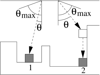
Figure 1: Discrete model. SOS shadowed ballistic deposition process. Particle 2 hits a column side, then falls down.

A typical result of this model is given figure 2. It is obtained for a periodic system of length $L=1024$ and $\theta_{max}=60^{\circ}$. Figure 2 gives the value $h(x,t)$ of the interface at different times. We observe that the system forms height flat structures with deep grooves in between. The column width increases with time while the number of column decreases. This columnar shape grows and persists at least until the end of the simulation. Figure 3 gives the distribution $f(h)$ of the height of the interface at time $t=20\,000$. It exhibits a single large peak for $h\sim 19\,000$ which corresponds to the top of the plateau, showing its flatness. The smallest values of $f(h)$ correspond to the bottom of the grooves which indeed remain at low values. This curve shape characterizes the columnar regime. Nevertheless it do not gives any information on the number of columns. It could be evaluated as in [17]. Because it is not the main interest of the paper, we turn now to the roughness $W(t)$, given figure 4, which is a more usual function in the deposition context. It exhibits two regimes. The first one until $t\sim 10$ for which $W\sim t^{.5}$ corresponds to a fluctuating interface. The second one for which $W\sim t$ corresponds to the columnar regime.

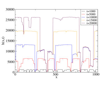
Figure 2: Discrete model. Interface $\,h(x,t)\,$ at time $t=1\,000$, 5 000, 10 000, 15 000 and 20 000 for $\theta_{max}=60^{\circ}$ and $L=1024$.

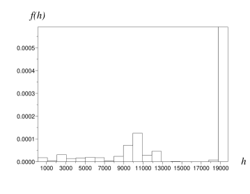
Figure 3: Distribution function of the interface height $h(x,t)$ plotted figure 2 at time $t=15\,000$.

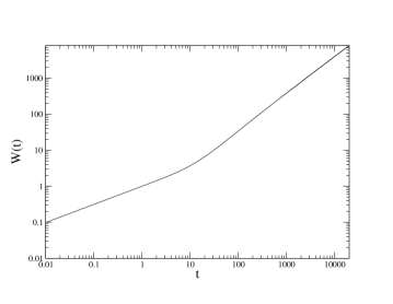
Figure 4: Time evolution of the roughness $W(t)$ for the simulation the results of which are given figure 2.

It has been recognized that, if a relaxation term is introduced, the columnar aspect is less strong and completely disappear if it is too high [18].

Now let us turn to a continuous model. The following model, which include shadowing effects, has been proposed by Karunasiri et al [2].

$$\frac{\partial h}{\partial t}=\nu\nabla^{2}h+\frac{\lambda}{2}(\nabla h)^{2}+R\Omega(x,\{h\})+\eta$$ (1)

which is a KPZ equation for which the deterministic deposition term $R$ is multiplied by the solid angle $\Omega(x,\{h\})$ which modelizes the shadowing effect. $\Omega(x,\{h\})$ is the solid angle subtended by the target surface seen from a point $x$ on the interface height $h(x,t)$ (see figure 5(a)). It is evaluated as in reference [2]. $\nu$ is the diffusion coefficient which is constant and $\eta$ the usual noise the mean of which, at time $t$, is equal to zero and the correlation given by $<\eta(x,t)\eta(x^{\prime},t^{\prime})>=2D\delta(x,x^{\prime})\delta(t,t^{\prime})$. Because we are only interested in the shadowing term effect, we reduce the analysis to this sole aspect, as we do for the Monte-Carlo simulations and consequently study the following equation :

$$\frac{\partial h}{\partial t}=R\Omega(x,\{h\})+\eta$$ (2)

Figure 5: Shadowing process : comparison between continuous (a) and discrete (b,c) models. Discrete model : the point at the bottom of a column receives particles if it is seen by the target (b) or if the side of the column is seen by the target (c).

Equation (2) is numerically integrated using a finite difference method with an explicit scheme. The time step $\Delta t=0.05$, the spatial step $\Delta x=1$, $R=1$ and we use periodic boundary conditions. At each integration time step the exposure angle $\Omega$ is compute for each point, then normalized with the mean value obtained at that time. This insure that the deposition rate is indeed constant and that each unit of time a single layer is growing on average.

Figures 6 gives the surface morphologies obtained at time $t=100$, $200$ and $300$ for a surface length $L=1024$. Indeed the shape of $h(x,t)$ is very different from the one obtained with the discrete model previously discussed. We do not have plateau but instead very high peaks. As the simulation goes on, a single peak emerges. Nevertheless this last effect is due to the finite size of the system.

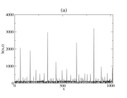
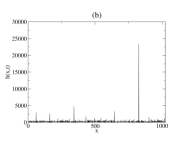
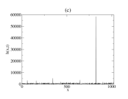
Figure 6: Interface $\,h(x,t)\,$ for a continuous model with shadowing deposition at time $t=100$ (a), $t=300$ (b), $t=500$ (c).

In order to improve continuous models, this difference has to be explained. For these models, the height of a site increases proportional to its exposure angle. This angle reaches $\pi$, and is maximum for the highest sites. By contrast, small height sites received less particles. More the difference is, less important is the increase rate for these sites. For example at time $t=500$, all points (except the single highest peak) have small exposure angle and then do not grow up very much while the peak quickly increases. The situation is the same for the discrete model except for sites which are at the bottom of a column. In fact for these sites, particles come directly from the source if they are in the correct exposure angle (figure 5(b)) but also fall down from the side of the column (see figure 5(c)).

It is possible to check this hypothesis by performing a peculiar discrete model. Now if a particle hit the edge of a column it is removed and consequently cannot fall down. Figures 7 show the height $h(x,t)$ of the interface at time $t=100$, 300 and 500. Indeed these figures are very similar to those obtained with the continuum model with shadowing (figures 6). Except to get a discrete model that mimic the continuous one, there is no physical reason for that process. Nevertheless it shows that the shadowing introduced in the continuous model is not enough to produce columnar shape deposit, and in addition it also shows the importance of the particle flux which fall down from the edges of the columns. This suggests the introduction of a stronger relaxation at the top of the column than at their bottom in the continuous model.

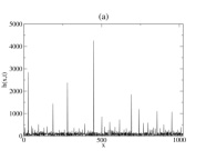
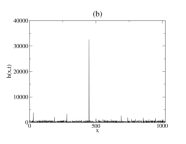
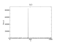
Figure 7: Discrete model. Interface height for a periodic system of length $L=1024$, at time $t=100$ (a), $t=300$ (b), $t=500$ (c). Particles which are hitting the side of a column are removed.

3 Continuous model driving to columnar shape deposit

We propose the following stochastic differential equation where the main ingredients are a non-linear shadowing effects and a anisotropic diffusion :

$$\frac{\partial h}{\partial t}=g(\Omega(x,\{h\}))\,(R\,\sqrt{1+|\nabla(h)|^{2}}+\nu\nabla^{2}h+\eta)$$ (3)

In this equation $g(\Omega)$ is a given function of the solid angle $\Omega$. The square root term $\sqrt{1+|\nabla(h)|^{2}}$ describes the fact that the local deposit grows normally to the interface. Here we do not make a first order approximation, as in [16], because, as we are looking for columnar shape deposit, the spatial variation of the height $h$ could be large. The fact that the solid angle, which modelizes the shadowing, is in factor the the right hand term. It will obviously increase the deposit rate for surfaces which are not shadowed (mainly for large value of $h$) and make it smaller for shadowed one (for small value of $h$). The diffusion is also affected by the shadowing. It has been recognized in section 2 that particles which fall down a column side increases the width of this column. This strong migration of particles from the side to the bottom of a column suggests this anisotropic diffusion. Moreover, in order to increase the shadowing effect, we take $g(\Omega)=\Omega^{2}$.

Equation (3) is integrated using the following explicit scheme:

$$h_{i}^{n+1} = h_{i}^{n}+\left(\Omega_{i}^{n}\right)^{2}\,\left[\Delta t\,R\,\sqrt{1+\left(\frac{h_{i+1}^{n}-h_{i-1}^{n}}{2\,\Delta x}\right)^{2}}\right.$$

$$+\frac{\nu\,\Delta t}{\Delta x^{2}}\,(h_{i+1}^{n}-2\,h_{i}^{n}+h_{i-1}^{n})+\left.\sqrt{\frac{2\,D\,\Delta t}{\Delta x}}\,\,\varepsilon\right]$$

with the notation $h_{i}^{n}=h(i\,\Delta x,n\,\Delta t)$, $\varepsilon$ is a random number picked with the uniform distribution between $[-1,1[$.

A plane wave analysis with a perturbation $h=h_{1}\exp(i(kx-\omega t))$, on the linearized version of equation (3), gives the following dispersion relation

$$-i\omega=2\frac{\alpha\,R}{\bar{\Omega}}\,k-\nu\,k^{2},$$ (5)

where $\bar{\Omega}$ is the mean value of the solid angle and $\alpha\sim.7$. With $\omega=\omega_{R}+i\omega_{I}$, equation (5) shows that the modes $k<k_{*}=2\alpha R/(\bar{\Omega}\nu)$ are unstable. Then, the noise trigger the instability and drives the system into a strong non-linear regime. Then, as shown figure 8, which gives the evolution of the interface profile at different times for $\Delta t=0.01$, $\Delta x=1$, $D=1$, $\nu=1$ and $R=1$, as time increases, a columnar deposit shape is observed. The competition between the shadowing deposition, which favors the emergence of a single structure (see figure 6), and the anisotropic diffusion, which propagate particles near the edges, keeps at least for the simulation time ($t=4\,000$) the columnar regime. Indeed figure 8 shows the formation of higher and higher columns. Moreover, most of the columns formed at the beginning of the simulation are still present at the end. The height distribution function (figure 9), computed at $t=4\,000$, is very similar to the one obtained with the discrete model and shows a strong peak for $h\sim 5\,000$ which correspond to the top of the columns. The time evolution of the roughness $W$ of the interface is given figure 10. It shows the existence of different regimes. The first one, for $t<1$ is driven by the fluctuations and $W$ scales as $t^{1/2}$. For the second one ($1<t<100$), diffusion induced a relative reduction of the roughness which scales as $t^{.4}$. Then, because of the shadowing instability described above, sharp canyons appear and the roughness quickly increases. Finally, after $t\sim 1000$, the columnar regime appears and gives $W\sim t$ as in the discrete model.

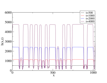
Figure 8: Continuous model. Snapshot of the interface given by the non-linear shadowing anisotropic diffusion model given by equation (3) at time $t=500$, 1 000, 2 000 and 4 000.

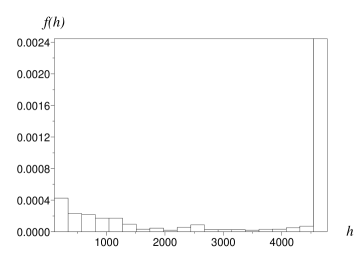
Figure 9: height distribution function of the interface corresponding to figure 8 at $t=4\,000$.

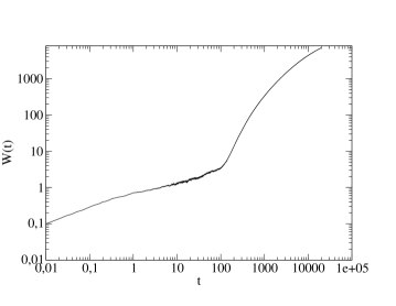
Figure 10: Continuous model. Time evolution of the roughness $W(t)$.

4 Discussion and Conclusion

In the past, both discrete and continuous models have been proposed to describe columnar shape deposit as those observed in plasma sputter deposition. Discrete models implying shadowing process, as the one established by Roland and Guo [3], indeed show the formation of larger and larger plateau as time increases. They also proposed a continuous model for which, each point of the interface received a flux of particles proportional to the local exposure angle. Then the interface obtained presents peaks but no columns as the discrete model do. We show that these two shadowing processes are not equivalent. For the discrete one, points which are at the bottom of columns received all the particles which are hitting the edges. There is no correspondence of such a process in the current continuous model. Nevertheless if we remove particles which are hitting the edges in discrete simulations, then the two types of models, for which only the shadowing deposition is taken into account, give the same kind of results : strong peaks appear and a single one dominated the others as time increases (due to finite size effects). It has to be notice that the flux of particles which fall down the edges of the column formed by the discrete model is not equivalent to a relaxation for the continuous one. This last term has a smooth effect. Nevertheless it suggests to introduce an anisotropic diffusion.

To conclude, we have proposed a new continuous model for which main ingredients are a non-linear shadowing deposit (proportional to the square of the local exposure angle $\Omega$) and an anisotropic diffusion. The numerical simulation results indeed show the formation of height columns, with sharp edges. Furthermore, numerical simulations show that it is necessary to deal with a nonlinear shadowing to obtain columnar shape deposit.

References

- [1] G. S. Bales, R. Bruinsma, E. A. Eklund, R. P. U. Karunasiri, J. Rudnick, A. Zangwill, Growth and Erosion of Thin Solid Films, Science 249, 1990, pp 264–268
- [2] R.P.U. Karunasiri, R. Bruinsma, J. Rudnick, Thin film and the shadow instability, Phys. Rev. Let. 62 7, 1989, pp 788–790
- [3] C. Roland, H. Guo, Interfacial Growth with a shadow instability Phys. Rev. Lett. 66 ,1991, pp 2104–2107
- [4] P.I. Tamborenea and S. Das Sarma, Surface-diffusion-driven kinetic growth on one-dimensional substrates, Phys Rev E, 48 4, 1993, pp 2575–2594
- [5] B. Meng, W.H. Weinberg, Dynamical Monte-Carlo studies of molecular beam epitaxial growth models : interfacial scaling and morphology, Surface Science 364, 1996, pp 151–163
- [6] K.A. Fichthorn, W.H. Weinberg, Theoretical foundations of dynamical Monte-Carlo simulations, J. Chem. Phys. 95 2, 1991, pp 1090–1096
- [7] S. Das Sarma, C. J. Lanczycki, R. Kotlyar, S. V. Ghaisas Scale invariance and dynamical correlations in growth models of molecular beam epitaxy, Phys. Rev. E 53, 1996, 359–389
- [8] M. Rost and J. Krug, Coarsening of surface structures in unstable epitaxial growth Phys. Rev. E 55, 3952-3957
- [9] J. G. Amar and F. Family, Numerical solution of a continuous equation for interface growth in 2+1 dimensions, Phys. Rev. A 41, 1992, 3399–3402
- [10] W. M. Tong and R. S. Williams, Kinetics of surface growth: Phenomenology, Scaling, Mechanisms of Smoothening and Roughening, Ann. Rev. Phys. Chem. 45, 1994, pp 401–438
- [11] A.-L. Barabasi, H. E. Stanley: Fractal Concepts in Surface Growth (Cambridge University Press, Cambridge 1995)
- [12] T. Witten and L. Sander, Diffusion-limited aggregation, Phys. Rev. B 3 27, 1983, pp 5686 -5697
- [13] M. Lagües, A. Lesne, Invariances d’échelle, des changements d’état à la turbulence, Belin, 2003, ISBN 2-7011-3175-8
- [14] S.F. Edward, D.R. Wilkinson, The surface statistics of a granular aggregate, Proc. Roy. Soc. A 381, 1982, pp 17–31
- [15] K. Park and B. N. Kahng, Exact derivation of the Kardar-Parisi-Zhang equation for the restricted solid-on-solid model, Phys. Rev. E 51 1, 1995, pp 796–798
- [16] M. Kardar, G. Parisi, Y.-C. Zhang, Dynamic scaling of growing interface, Phys. Rev. Letters 56 9, 1986, pp 889–892
- [17] J.H. Yao, C. Roland, H. Guo, Interfacial dynamics with long-range screening, Phys. Rev. A 45 6, 1992, pp 3903–3912
- [18] J.H. Yao, H. Guo, Shadowing in the three dimensions, Phys. Rev. E 47 2, 1993, pp 1007–1011
- [19] J. T. Drotar, Y.-P. Zhao, T.-M Lu, G.-C. Wang, Surface roughening growth and etching in 2+1 dimensions Phys. Rev. B 62 3, 2000, pp 2118–2125