Any $l$-state solutions of the Hulthén potential by the asymptotic iteration method

Abstract

In this article, we present the analytical solution of the radial Schrödinger equation for the Hulthén potential within the framework of the asymptotic iteration method by using an approximation to the centrifugal potential for any $l$ states. We obtain the energy eigenvalues and the corresponding eigenfunctions for different screening parameters. The wave functions are physical and energy eigenvalues are in good agreement with the results obtained by other methods for different $\delta$ values. In order to demonstrate this, the results of the asymptotic iteration method are compared with the results of the supersymmetry, the numerical integration, the variational and the shifted $1/N$ expansion methods.

I Introduction

Over the last decades, the energy eigenvalues and corresponding eigenfunctions between interaction systems have raised a great deal of interest in relativistic quantum mechanics as well as in non-relativistic quantum mechanics. The exact solution of the wave equations (relativistic or non-relativistic) are very important since the wave function contains all the necessary information regarding the quantum system under consideration. Analytical methods such as the supersymmetry (SUSY) susy and the Nikiforov-Uvarov method (NU) Nifikorov have been used to solve the wave equations exactly or quasi-exactly for non zero angular momentum quantum number ($l\neq 0$) by means of a given potential. The radial Schrödinger equation for the Hulthèn potential is solved exactly by using several techniques hulthen ; nu1s ; fluge for $l=0$. For the case $l\neq 0$, the effective Hulthén potential can not be solved exactly, but a number of methods have been used to find the bound state energy eigenvalues numerically Varshni and quasi-analytically such as the variational Varshni , perturbation perturbation , shifted $1/N$ expansion shift , NU nu2s and SUSY susy1 methods. The Hulthén potential hulthen is one of the important short-range potentials in physics and it potential has been applied to a number of areas such as nuclear and particle physics, atomic physics, condensed matter and chemical physics (see Varshni and the references therein). Therefore, it would be interesting and important to solve the non-relativistic radial Schrödinger equation for this potential for $l\neq 0$, since it has been extensively used to describe the bound and the continuum states of the interaction systems. Recently, an alternative method, called as the asymptotic iteration method (AIM), has been developed by Çiftçi et al. hakanaim1 ; hakanaim2 for solving second-order homogeneous linear differential equations and it has been applied to solve the non-relativistic radial Schrödinger equation or the relativistic Dirac equation.

In this paper, we aim to solve the Hulthén potential to obtain the energy eigenvalues and corresponding eigenfunctions for any $l$ states. In the next section, AIM is introduced. Then, in section III, the Schrödinger equation is solved by using AIM for the Hulthén potential for any $l$ states and our AIM results are given in comparison with the results of the numerical integration Varshni , the variational Varshni , the shifted $1/N$ expansion shift and the SUSY susy1 methods. Finally, section IV is devoted to the summary and conclusion.

II Overview of the Asymptotic Iteration Method

II.1 Energy Eigenvalues

AIM is briefly outlined here and the details can be found in references hakanaim1 ; hakanaim2 ; bayrakJPA . AIM is proposed to solve the second-order differential equations of the form

$$y^{\prime\prime}=\lambda_{0}(x)y^{\prime}+s_{0}(x)y$$ (1)

where $\lambda_{0}(x)\neq 0$ and the prime denotes the derivative with respect to $x$. The variables, $s_{0}(x)$ and $\lambda_{0}(x)$, are sufficiently differentiable. The differential equation (1) has a general solution hakanaim1

$$y(x)=exp\left(-\int^{x}\alpha(x_{1})dx_{1}\right)\left[C_{2}+C_{1}\int^{x}exp\left(\int^{x_{1}}[\lambda_{0}(x_{2})+2\alpha(x_{2})]dx_{2}\right)dx_{1}\right]$$ (2)

for sufficiently large $k$, $k>0$, if

$$\frac{s_{k}(x)}{\lambda_{k}(x)}=\frac{s_{k-1}(x)}{\lambda_{k-1}(x)}=\alpha(x),\quad k=1,2,3,\ldots$$ (3)

where

$$\lambda_{k}(x) = \lambda_{k-1}^{\prime}(x)+s_{k-1}(x)+\lambda_{0}(x)\lambda_{k-1}(x)\quad$$

$$s_{k}(x) = s_{k-1}^{\prime}(x)+s_{0}(x)\lambda_{k-1}(x),\quad\quad\quad\quad k=1,2,3,\ldots$$ (4)

Note that one can also start the recurrence relations from $k=0$ with the initial conditions $\lambda_{-1}=1$ and $s_{-1}=0$ fernandez . For a given potential such as the Hulthén, the radial Schrödinger equation is converted to the form of equation (1). Then, s${}_{0}(x)$ and $\lambda_{0}(x)$ are determined and s${}_{k}(x)$ and $\lambda_{k}(x)$ parameters are calculated by the recurrence relations given by equation (II.1).

The termination condition of the method in equation (3) can be arranged as

$$\Delta_{k}(x)=\lambda_{k}(x)s_{k-1}(x)-\lambda_{k-1}(x)s_{k}(x)=0\quad\quad k=1,2,3,\ldots$$ (5)

The energy eigenvalues are obtained from the roots of the equation (5) if the problem is exactly solvable. If not, for a specific $n$ principal quantum number, we choose a suitable $x_{0}$ point, determined generally as the maximum value of the asymptotic wave function or the minimum value of the potential bayrakIJQC ; hakanaim1 ; barakat ; fernandez , and the approximate energy eigenvalues are obtained from the roots of this equation for sufficiently great values of $k$ with iteration.

II.2 Energy Eigenfunctions

In this study, we seek the exact solution of the radial Schrödinger equation for which the relevant second order homogenous linear differential equation takes the following general form hakanaim2 ,

$${y}^{\prime\prime}=2\left({\frac{ax^{N+1}}{1-bx^{N+2}}-\frac{\left({t+1}\right)}{x}}\right){y}^{\prime}-\frac{w_{k}^{t}(N)x^{N}}{1-bx^{N+2}}y,\,\,\,\,\,\,\,\,\,\,\ 0<x<\infty$$ (6)

If this equation is compared to equation (1), it entails the following expressions

$$\lambda_{0}(x)=2\left({\frac{ax^{N+1}}{1-bx^{N+2}}-\frac{\left({t+1}\right)}{x}}\right),\hskip 28.45274pts_{0}(x)=-\frac{w_{k}^{t}(N)x^{N}}{1-bx^{N+2}}$$ (7)

$a$ and $b$ are constants and $w_{k}^{t}(N)$ can be determined from the condition (3) for $k=0,1,2,3,...$ and $N$=-1,0,1,2,3,… as follows:

$$w_{k}^{t}(-1) = k\left({2a+2bt+(k+1)b}\right)$$ (8)

$$w_{k}^{t}(0) = 2k\left({2a+2bt+(2k+1)b}\right)$$ (9)

$$w_{k}^{t}(1) = 3k\left({2a+2bt+(3k+1)b}\right)$$ (10)

$$w_{k}^{t}(2) = 4k\left({2a+2bt+(4k+1)b}\right)$$ (11)

$$w_{k}^{t}(3) = 5k\left({2a+2bt+(5k+1)b}\right)$$ (12)

$$\ldots\emph{etc}$$

Hence, these formule are easily generalized as,

$$w_{k}^{t}(N)=b\left({N+2}\right)^{2}k\left({k+\frac{\left({2t+1}\right)b+2a}{\left({N+2}\right)b}}\right)$$ (13)

The exact eigenfunctions can be derived from the following generator:

$$y_{n}(x)=C_{2}\exp\left({-\int\limits^{x}{\frac{s_{k}(x^{\prime})}{\lambda_{k}(x^{\prime})}dx^{{}^{\prime}}}}\right)$$ (14)

where $k\geq n$, $n$ represents the radial quantum number and $k$ shows the iteration number. For exactly solvable potentials, the radial quantum number $n$ is equal to the iteration number $k$ and the eigenfunctions are obtained directly from equation (14). For nontrivial potentials that have no exact solutions, $k$ is always greater than $n$ in these numerical solutions and the approximate energy eigenvalues are obtained from the roots of equation (5) for sufficiently great values of $k$ with iteration. It should be pointed out that $\alpha(x)$ given by equation (3) is equal to zero for the ground state. Therefore, using equation (3) with (7) in equation (14), the eigenfunctions are obtained as follows,

$$y_{0}(x) = C_{2}$$

$$y_{1}(x) = -C_{2}(N+2)\sigma\left({1-\frac{b\left({\rho+1}\right)}{\sigma}x^{N+2}}\right)$$

$$y_{2}(x) = C_{2}(N+2)^{2}\sigma\left({\sigma+1}\right)\left({1-\frac{2b\left({\rho+2}\right)}{\sigma}x^{N+2}+\frac{b^{2}\left({\rho+2}\right)\left({\rho+3}\right)}{\sigma\left({\sigma+1}\right)}x^{2(N+2)}}\right)$$

$$y_{3}(x) = -C_{2}\frac{\sigma\left({\sigma+1}\right)\left({\sigma+2}\right)}{\left({N+2}\right)^{-3}}$$

$$\times \left({1-\frac{3b\left({\rho+3}\right)}{\sigma}x^{N+2}+\frac{3b^{2}\left({\rho+3}\right)\left({\rho+4}\right)}{\sigma\left({\sigma+1}\right)}x^{2(N+2)}-\frac{b^{3}\left({\rho+3}\right)\left({\rho+4}\right)\left({\rho+5}\right)}{\sigma\left({\sigma+1}\right)\left({\sigma+2}\right)}x^{3\left({N+2}\right)}}\right)$$

$$\ldots\emph{etc}$$

Finally, the following general formula for the exact solutions $y_{n}(x)$ is obtained as,

$$y_{n}(x)=\left({-1}\right)^{n}C_{2}(N+2)^{n}\left(\sigma\right)_{n}{}_{2}F_{1}(-n,\rho+n;\sigma;bx^{N+2})$$ (15)

It is important to note that square integrable one in $L^{2}$ is this total wave function which is the asymptotic form of the wave function times $y_{n}(x)$ given by equation (14). Here, $(\sigma)_{n}$=$\frac{\Gamma({\sigma+n})}{\Gamma(\sigma)},\quad\sigma$ = $\frac{2t+N+3}{N+2}$  and  $\rho$ = $\frac{({2t+1})b+2a}{({N+2})b}$. The $(\sigma)_{n}$ and the ${}_{2}F_{1}$ are known as the Pochhammer symbol and the Gauss hypergeometric function, respectively.

III Calculation of the Energy Eigenvalues and Eigenfunctions

The motion of a particle with the mass $M$ in the spherically symmetric potential is described in the spherical coordinates by the following Schrödinger equation:

$$\frac{-\hbar^{2}}{2M}\left(\frac{\partial^{2}}{\partial r^{2}}+\frac{2}{r}\frac{\partial}{\partial r}+\frac{1}{r^{2}}\left[\frac{1}{\sin\theta}\frac{\partial}{\partial\theta}\left(\sin\theta\frac{\partial}{\partial\theta}\right)+\frac{1}{\sin^{2}\theta}\frac{\partial^{2}}{\partial\phi^{2}}\right]+V(r)\right)\Psi_{nlm}(r,\theta,\phi)=E\Psi_{nlm}(r,\theta,\phi)$$ (16)

Defining $\Psi_{nlm}(r,\theta,\phi)=R_{nl}(r)Y_{lm}(\theta,\phi)$, we obtain the radial part of the Schrödinger equation:

$$\left(\frac{d^{2}}{d{r}^{2}}+\frac{2}{r}\frac{d}{dr}\right)R_{nl}(r)+\frac{2M}{\hbar^{2}}\left[E-V(r)-\frac{l(l+1)\hbar^{2}}{2Mr^{2}}\right]R_{nl}(r)=0$$ (17)

It is sometimes convenient to define $R_{nl}(r)$ and the effective potential as follows

$$R_{nl}(r)=\frac{u_{nl}(r)}{r},\quad V_{eff}=V(r)+\frac{l(l+1)\hbar^{2}}{2Mr^{2}}$$ (18)

Since

$$\left(\frac{d^{2}}{d{r}^{2}}+\frac{2}{r}\frac{d}{dr}\right)\frac{u_{nl}(r)}{r}=\frac{1}{r}\frac{d^{2}}{d{r}^{2}}u_{nl}(r)$$ (19)

The radial Schrödinger equation fluge given by equation (17) follows that

$$\frac{d^{2}u_{nl}(r)}{d{r}^{2}}+\frac{2M}{\hbar^{2}}\left[E-V_{eff}\right]u_{nl}(r)=0$$ (20)

The Hulthén potential hulthen is given by

$$V_{H}(r)=-Ze^{2}\delta\frac{e^{-\delta r}}{1-e^{-\delta r}}$$ (21)

where Z and $\delta$ are respectively the atomic number and the screening parameter, determining the range for the Hulthén potential. The Hulthén potential behaves like the Coulomb potential near the origin $(r\longrightarrow 0)$, but in the asymptotic region $(r\gg 1)$, the Hulthén potential decreases exponentially, so its capacity for bound states is smaller than the Coulomb potential. However, for small values of the screening parameter $\delta$, the Hulthén potential becomes the Coulomb potential given by $V_{C}=-\frac{Ze^{2}}{r}$. The effective Hulthén potential is

$$V_{eff}(r)=V_{H}(r)+V_{l}=-Ze^{2}\delta\frac{e^{-\delta r}}{1-e^{-\delta r}}+\frac{l(l+1)\hbar^{2}}{2Mr^{2}}$$ (22)

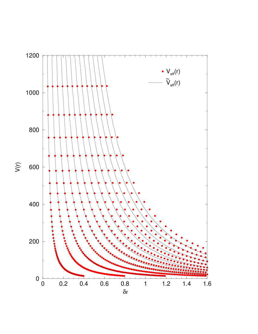
Figure 1: The variation of the effective Hulthén ${V}_{eff}(r)$ and the approximate effective Hulthén potentials $\widetilde{V}_{eff}(r)$ with respect to the $\delta r$ for various values of the screening parameter. The parameters are in atomic units $(\hbar=e=m=1)$ and $\delta$ change from 0.4 to 5.2 in steps of 0.4.

where $V_{l}=\frac{l(l+1)\hbar^{2}}{2Mr^{2}}$ is known as the centrifugal term. This effective potential can not be solved analytically for $l\neq 0$ because of the centrifugal term. Therefore, we must use an approximation for the centrifugal term similar to other authors susy1 ; nu2s ; other1 ; other2 ; other3 ; other4 . In this approximation, $\frac{1}{r^{2}}=\delta^{2}\frac{e^{-\delta r}}{(1-e^{-\delta r})^{2}}$ is used for the centrifugal term. As shown in figure 1, this approximation is only valid for small $\delta r$ and it breaks down in the high-screening region. For small $\delta r$, $\widetilde{V}_{eff}(r)$ is very well approximated to $V_{eff}(r)$ and the Schrödinger equation for this approximate potential is solvable analytically. So, the effective potential becomes

$$\widetilde{V}_{eff}(r)=-Ze^{2}\delta\frac{e^{-\delta r}}{1-e^{-\delta r}}+\frac{l(l+1)\hbar^{2}\delta^{2}}{2M}\frac{e^{-\delta r}}{(1-e^{-\delta r})^{2}}$$ (23)

Instead of solving the radial Schrödinger equation for the effective Hulthén potential $V_{eff}(r)$ given by equation (22), we now solve the radial Schrödinger equation for the new effective potential $\widetilde{V}_{eff}(r)$ given by equation (23). Inserting this new effective potential into equation (20) and using the following ansatzs in order to make the differential equation more compact

$$-\varepsilon^{2}=\frac{2ME}{\hbar^{2}\delta^{2}},\quad\beta^{2}=\frac{2MZe^{2}}{\hbar^{2}\delta},\quad\delta r=x$$ (24)

The radial Schrödinger equation takes the following form:

$$\frac{d^{2}u_{nl}(x)}{dx^{2}}+\left[-\varepsilon^{2}+\beta^{2}\frac{e^{-x}}{(1-e^{-x})}-l(l+1)\frac{e^{-x}}{(1-e^{-x})^{2}}\right]u_{nl}(x)=0$$ (25)

If we rewrite equation (25) by using a new variable of the form $z=e^{-x}$, we obtain

$$\frac{d^{2}u_{nl}(z)}{dz^{2}}+\frac{1}{z}\frac{du_{nl}(z)}{dz}+\left[-\frac{\varepsilon^{2}}{z^{2}}+\frac{\beta^{2}}{z(1-z)}-\frac{l(l+1)}{z(1-z)^{2}}\right]u_{nl}(z)=0$$ (26)

In order to solve this equation with AIM, we should transform this equation to the form of equation (1). Therefore, the reasonable physical wave function we propose is as follows

$$u_{nl}(z)=z^{\varepsilon}(1-z)^{l+1}f_{nl}(z)$$ (27)

If we insert this wave function into equation (26), we have the second-order homogeneous linear differential equations as in the following form

$$\frac{d^{2}f_{nl}(z)}{dz^{2}}=\left[\frac{(2\varepsilon+2l+3)z-(2\varepsilon+1)}{z(1-z)}\right]\frac{df_{nl}(z)}{dz}+\left[\frac{(2\varepsilon+l+2)l+2\varepsilon-\beta^{2}+1}{z(1-z)}\right]f_{nl}(z)$$ (28)

which is now amenable to an AIM solution. By comparing this equation with equation (1), we can write the $\lambda_{0}(z)$ and $s_{0}(z)$ values and by means of equation (II.1), we may calculate $\lambda_{k}(z)$ and $s_{k}(z)$. This gives:

$$\lambda_{0}(z) = \left(\frac{(2\varepsilon+2l+3)z-(2\varepsilon+1)}{z(1-z)}\right)$$

$$s_{0}(z) = \left(\frac{(2\varepsilon+l+2)l+2\varepsilon-\beta^{2}+1}{z(1-z)}\right)$$

$$\lambda_{1}(z) = \frac{2+6\,\varepsilon-7\,z-2\,lz-{\beta}^{2}z+12\,{z}^{2}l-18\,\varepsilon\,z-6\,\varepsilon\,zl}{{z}^{2}\left(-1+z\right)^{2}}$$

$$+ \frac{12\,\varepsilon\,{z}^{2}+11\,{z}^{2}+4\,{\varepsilon}^{2}+{l}^{2}z+{\beta}^{2}{z}^{2}+4\,{\varepsilon}^{2}{z}^{2}-8\,{\varepsilon}^{2}z+6\,\varepsilon\,{z}^{2}l+3\,{l}^{2}{z}^{2}}{{z}^{2}\left(-1+z\right)^{2}}$$

$$s_{1}(z) = {\frac{\left(2\,l+2\,\varepsilon-{\beta}^{2}+2\,\varepsilon\,l+{l}^{2}+1\right)\left(-2+5\,z+2\,\varepsilon\,z+2\,lz-2\,\varepsilon\right)}{{z}^{2}\left(-1+z\right)^{2}}}$$

$$\ldots\emph{etc}$$ (29)

Combining these results with the quantization condition given by equation (5) yields

$$s_{0}\lambda_{1}-s_{1}\lambda_{0} =0 \,\,\,\,\,\,\Rightarrow\,\,\,\,\,\,\varepsilon_{0}=\frac{\beta^{2}-1-2l-l^{2}}{2(l+1)},\quad for\quad k=1$$

$$s_{1}\lambda_{2}-s_{2}\lambda_{1} =0 \,\,\,\,\,\,\Rightarrow\,\,\,\,\,\,\varepsilon_{1}=\frac{\beta^{2}-4-4l-l^{2}}{2(l+2)},\quad for\quad k=2$$

$$s_{2}\lambda_{3}-s_{3}\lambda_{2} =0 \,\,\,\,\,\,\Rightarrow\,\,\,\,\,\,\varepsilon_{2}=\frac{\beta^{2}-9-6l-l^{2}}{2(l+3)},\quad for\quad k=3$$ (30)

$$\ldots\emph{etc}$$

When the above expressions are generalized, the eigenvalues turn out as

$$\varepsilon_{nl}=\left(\frac{\beta^{2}-(n+l+1)^{2}}{2(n+l+1)}\right)\hskip 28.45274ptn,l=0,1,2,3,...$$ (31)

Using equation (24), we obtain the energy eigenvalues E_nl,

$$E_{nl}=-\frac{\hbar^{2}}{2M}\left[\frac{MZe^{2}}{\hbar^{2}(n+l+1)}-\frac{(n+l+1)\delta}{2}\right]^{2}\hskip 28.45274pt$$ (32)

In the atomic units $(\hbar=M=e=1)$ and for Z = 1, equation (32) turns out to be

$$E_{nl}=-\frac{1}{2}\left[\frac{1}{(n+l+1)}-\frac{(n+l+1)\delta}{2}\right]^{2}\hskip 28.45274pt$$ (33)

In order to test the accuracy of equation (33), we calculate the energy eigenvalues for $Z=1$, any $n$ and $l$ quantum numbers and several values of the screening parameter. AIM results are compared with the results of the numerical integration Varshni , the variational Varshni , the shifted $1/N$ expansion shift and the SUSY susy1 methods in Table 1 and Table 2. As it can be seen from the results presented in these tables, the AIM results are in good agrement with the results of the other methods for the small $\delta$ values. For large $\delta$ values, there are differences between our results and the results of others. This difference is due to the $\widetilde{V}_{eff}(r)$ potential, which we have used to approximate the $V_{eff}(r)$ potential. As it is seen from figure 1, for large $\delta r$ values, the discrepancy becomes apparent between our $\widetilde{V}_{eff}(r)$ and the true $V_{eff}(r)$ potentials. This gives rise to the differences for the eigenvalues presented in Tables 1 and 2 at large $\delta$ values.

Now, as indicated in Section II, we can determine the corresponding wave functions by using equation (15). When we compare equation (6) and equation (28), we find $N=-1$, $b=1$, $a=l+1$, and $t=\frac{2\varepsilon-1}{2}$. Therefore, we find $\rho=2(\varepsilon+l+1)$ and $\sigma=2\varepsilon+1$. So, we can easily find the solution for $f_{nl}(z)$, for the energy eigenvalue equation (32) by using equation (15).

$$f_{nl}(z)=(-1)^{n}\frac{\Gamma(2\varepsilon_{n}+n+1)}{\Gamma(2\varepsilon_{n}+1)}{{}_{2}}F_{1}(-n,2\varepsilon_{n}+2l+2+n;2\varepsilon_{n}+1;z)$$ (34)

Thus, we can write the total radial wave function as below,

$$u_{nl}(z)=Nz^{\varepsilon_{n}}(1-z)^{l+1}{{}_{2}}F_{1}(-n,2(\varepsilon_{n}+l+1)+n;2\varepsilon_{n}+1;z)$$ (35)

where $N$ is the normalization constant.

IV Conclusion

We have shown an alternative method to obtain the energy eigenvalues and corresponding eigenfunctions of the Hulthén potential within the framework of the asymptotic iteration method for any $l$ states. We have calculated the energy eigenvalues for the Hulthén potential with $Z=1$ and several values of the screening parameter. The wave functions are physical and energy eigenvalues are in good agreement with the results obtained by other methods. In order to demonstrate this, AIM results have been compared with the results of the numerical integration Varshni , the variational Varshni , the shifted $1/N$ expansion shift and the SUSY susy1 methods in Tables 1 and 2. For small $\delta$ values, AIM results are in good agreement with the results of the other methods, but in the high screening region, the agreement is poor. The reason is simply that when the $\delta r$ increases in the high screening region, the agreement between $V_{eff}(r)$ and $\widetilde{V}_{eff}(r)$ potentials decreases as shown in Figure 1. This problem could be solved by making a better approximation of the centrifugal term.

It should be pointed out that the asymptotic iteration method gives the eigenvalues directly by transforming the radial Schrödinger equation into a form of ${y}^{\prime\prime}$ =$\lambda_{0}(r){y}^{\prime}+s_{0}(r)y$. The wave functions are easily constructed by iterating the values of $s_{0}(r)$ and $\lambda_{0}(r)$. The asymptotic iteration method results in exact analytical solutions if there is and provides the closed-forms for the energy eigenvalues as well as the corresponding eigenfunctions. Where there is no such a solution, the energy eigenvalues are obtained by using an iterative approach bayrakIJQC ; barakat ; fernandez . As it is presented, AIM puts no constraint on the potential parameter values involved and it is easy to implement. The results are sufficiently accurate for practical purposes.

V REFERENCES

F. Cooper, A. Khare and U. Sukhatme, Phys. Rep. 251 (1995) 267.

A. F. Nikiforov and V. B. Uvarov, Special Functions of Mathematical Physics, Birkhäuser, Basel, (1988).

H. Ciftci, R. L. Hall and N. Saad, J. Phys. A: Math. Gen. 36 (2003) 11807.

H. Ciftci, R. L. Hall and N. Saad, J. Phys. A: Math. Gen. 38 (2005) 1147.

O. Bayrak and I. Boztosun, J. Phys. A: Math. Gen. 39 (2006) 6955.

L. Hulthén, Ark. Mat. Astron. Fys. 28A (1942) 5.

M. Akdaṣ, R. Sever, J. Molec. Struc. (Theochem) 710 (2004) 223.

S. Flügge, Practical Quantum Mechanics Vol. I, Springer, Berlin, (1994).

Y.P. Varshni, Phys. Rev. A 41 1990 4682

P. Matthys, H. De Meyer, Phys. Rev. A 38 (1988) 1168.

A.Z. Tang, F.T. Chan, Phys. Rev. A 35 (1987) 911.

S. M. Ikhdair and R. Sever, [arXiv:quant-ph/0508009].

B. Gonul, O. Ozer, Y. Cancelik and M. Kocak, Phys. Lett. A 275 (2000) 238.

R.L. Greene, C. Aldrich, Phys. Rev. A 14 (1976) 2363.

U. Myhrman, J. Phys. A: Math. Gen. 16 (1983) 263.

A. Bechlert, W Bühring, J. Phys. B: At. Mol. Opt. Phys. 21 (1988) 817.

Shang-Wu Qian, Bo-Wen Huang, and Zhi-Yu Gu, New Journal of Physics 4 (2002) 13.

O. Bayrak and I. Boztosun, Int. J. Quantum Chem. (2006), in press.
I. Boztosun, M. Karakoc, F. Yasuk and A. Durmus, J. Math. Phys. 47 (2006) 062301.

T. Barakat, J. Phys. A: Math. Gen. 39 (2006) 823.
T. Barakat, Phys. Lett. A344 (2005) 411.
T. Barakat, K. Abodayeh, A. Mukheimer, J. Phys. A: Math. Gen. 38 (2005) 1299.

F. M. Fernández, J. Phys. A: Math. Gen. 37 (2004) 6173.

$State$		$\delta$		AIM		SUSY susy1		Numerical Int. Varshni		Variational Varshni		Shifted $\frac{1}{N}$ shift
2p		0.025		0.1128125		0.1127605		0.1127605		0.1127605
		0.050		0.1012500		0.1010425		0.1010425		0.1010425		0.1010424
		0.075		0.0903125		0.0898478		0.0898478		0.0898478
		0.100		0.0800000		0.0791794		0.0791794		0.0791794		0.0791794
		0.150		0.0612500		0.0594415		0.0594415		0.0594415
		0.200		0.0450000		0.0418854		0.0418860		0.0418860		0.0418857
		0.250		0.0312500		0.0266060		0.0266111		0.0266108
		0.300		0.0200000		0.0137596		0.0137900		0.0137878
		0.350		0.0112500		0.0036146		0.0037931		0.0037734
3p		0.025		0.0437590		0.0437068		0.0437069		0.0437069
		0.050		0.0333681		0.0331632		0.0331645		0.0331645		0.03316518
		0.075		0.0243837		0.0239331		0.0239397		0.0239397
		0.100		0.0168056		0.0160326		0.0160537		0.0160537		0.01606772
		0.150		0.0058681		0.0043599		0.0044663		0.0044660
3d		0.025		0.0437587		0.0436030		0.0436030		0.0436030
		0.050		0.0333681		0.0327532		0.0327532		0.0327532		0.0327532
		0.075		0.0243837		0.0230306		0.0230307		0.0230307
		0.100		0.0168055		0.0144832		0.0144842		0.0144842		0.0144842
		0.150		0.0058681		0.0132820		0.0013966		0.0013894

Table 1: Energy eigenvalues of the Hulthén potential as a function of the screening parameter for 2p, 3p and 3d states in atomic units $(\hbar=m=e=1)$ and for $Z=1$.

$State$		$\delta$		AIM		SUSY susy1		Numerical Int. Varshni		Variational Varshni		Shifted $\frac{1}{N}$ shift
4p		0.025		0.0200000		0.0199480		0.0199489		0.0199489
		0.050		0.0112500		0.0110430		0.0110582		0.0110582		0.0110725
		0.075		0.0050000		0.0045385		0.0046219		0.0046219
		0.100		0.0012500		0.0004434		0.0007550		0.0007532
4d		0.025		0.0200000		0.0198460		0.0198462		0.0198462
		0.050		0.0112500		0.0106609		0.0106674		0.0106674		0.0106690
		0.075		0.0050000		0.0037916		0.0038345		0.0038344
4f		0.025		0.0200000		0.0196911		0.0196911		0.0196911
		0.050		0.0112500		0.0100618		0.0100620		0.0100620		0.0100620
		0.075		0.0050000		0.0025468		0.0025563		0.0025557
5p		0.025		0.0094531		0.0094011		0.0094036				0.0094087
		0.050		0.0028125		0.0026056		0.0026490
5d		0.025		0.0094531		0.0092977		0.0093037				0.0093050
		0.050		0.0028125		0.0022044		0.0023131
5f		0.025		0.0094531		0.0091507		0.0091521				0.0091523
		0.050		0.0028125		0.0017421		0.0017835
5g		0.025		0.0094531		0.0089465		0.0089465				0.0089465
		0.050		0.0028125		0.0010664		0.0010159
6p		0.025		0.0042014		0.0041493		0.0041548
6d		0.025		0.0042014		0.0040452		0.0040606
6f		0.025		0.0042014		0.0038901		0.0039168
6g		0.025		0.0042014		0.0036943		0.0037201

Table 2: Energy eigenvalues of the Hulthén potential as a function of the screening parameter for 4p, 4d, 4f, 5p, 5d, 5f ,5g, 6p, 6d, 6f and 6g states in atomic units $(\hbar=m=e=1)$ and for $Z=1$.