Nonsingular solutions of Hitchin’s equations for noncompact gauge groups

Abstract

We consider a general ansatz for solving the 2-dimensional Hitchin’s equations, which arise as dimensional reduction of the 4-dimensional self-dual Yang-Mills equations, with remarkable integrability properties. We focus on the case when the gauge group $G$ is given by a real form of $SL(2,\mathbb{C})$. For $G=SO(2,1)$, the resulting field equations are shown to reduce to either the Liouville, elliptic sinh-Gordon or elliptic sine-Gordon equations. As opposed to the compact case, given by $G=SU(2)$, the field equations associated with the noncompact group $SO(2,1)$ are shown to have smooth real solutions with nonsingular action densities, which are furthermore localized in some sense. We conclude by discussing some particular solutions, defined on $\mathbb{R}^{2}$, $S^{2}$ and $T^{2}$, that come out of this ansatz.

I Introduction

Yang-Mills theory has been a rich source of profound mathematical results in the past three decades. It has found applications in a wide variety of research areas, such as differential topology and algebraic geometry DK , representation theory Nak and in the theory of integrable systems H2 ; MW .

Usually, one considers the Yang-Mills self-duality equations for connections taking values on the Lie algebra of a compact real Lie group. So far, Yang-Mills instantons for complex or noncompact real Lie groups have received little attention (see for instance R ) and, to our knowledge, no general theory has been developed and the proper physical interpretation of such theory is yet to be understood, see gabor for a recent result in this direction. In this paper, we intend to provide motivation for the study of Yang-Mills theory with noncompact real Lie groups by remarking upon some rather interesting phenomena taking place on a two-dimensional gauge theory.

More precisely, let $G$ be a real Lie group with Lie algebra $\mathcal{G}$, and let $G^{\mathbb{C}}$ be its complexification. Let $A=A_{1}dx+A_{2}dy+A_{3}du+A_{4}dv$ be a $G$-connection 1-form defined on Euclidean $\mathbb{R}^{4}$, with Cartesian coordinates $(x,y,u,v)$. We are interested in the dimensionally reduced case where the fields depend only on $(x,y)$. In this case, it is known that the self-duality equations reduce to the so-called Hitchin’s equations hitchin :

$$F_{\tilde{A}} =-[\Phi,\Phi^{*}],$$ (1a)

$$d_{\tilde{A}}\Phi =0,$$ (1b)

where $\tilde{A}=A_{1}dx+A_{2}dy$ defines a connection over $\mathbb{R}^{2}$, $F_{\tilde{A}}$ is the curvature of $\tilde{A}$ and $\Phi=\frac{1}{2}(A_{3}-iA_{4})(dx+idy)$ can be thought of as a Higgs field. The anti-automorphism $*$ acts on $\mathcal{G}\otimes\Omega^{1}_{\mathbb{R}^{2}}\otimes\mathbb{C}$ as minus the identity on the first factor, $\mathcal{G}$, and as complex conjugation on the space of complex valued 1-forms, $\Omega^{1}_{\mathbb{R}^{2}}\otimes\mathbb{C}$. Equations (1) inherit the conformal invariance of the 4-dimensional Yang-Mills equations and can be considered on any Riemann surface $\Sigma$. It has been remarked that there are no smooth real solutions of the these equations for $\Sigma=\mathbb{R}^{2},S^{2},T^{2}$ (where $T^{2}$ is the 2-torus) and $G=SU(2)$ saclioglu ; hitchin .

In this paper, we obtain smooth real solutions of (1) for $\Sigma=\mathbb{R}^{2},S^{2},T^{2}$ and $G=SO(2,1)$, with nonsingular bounded action densities. It should be noted that the similar problem of finding solutions to the dimensionally reduced self-duality equations taking values in the complexified version $su(2)\otimes\mathbb{C}$ of $su(2)$ was addressed in the earlier saclioglu . Here, by employing a result of Donaldson donaldson which relates Hitchin pairs $(\tilde{A},\Phi)$ to flat $G^{\mathbb{C}}$-connections on $\Sigma$, we obtain an ansatz which turns out to be essentially the same as that of saclioglu . We show that this ansatz reduces the Hitchin’s equations to some classical integrable equations, namely the Liouville, the elliptic sinh-Gordon and the elliptic sine-Gordon equations. The first case (Liouville) was addressed, from a different perspective, already in saclioglu , where the author also showed that the strictly compact case leads to the sinh-Gordon equation (but in a different variant from that obtained here for $SO(2,1)$; see section IV). Moreover, we note that the strong link between Yang-Mills instantons and classical integrable equations is well known (see the book MW ), but that here it arises within the context of noncompact real Lie groups. The $U(n)$ Hitchin’s equations also lead to a celebrated completely integrable system, the Hitchin system H2 . It is remarkable that this link between Hitchin’s equations and integrable systems also arises when noncompact real Lie groups are considered.

II Algebraic preliminaries

Let $\{\tau_{1},\tau_{2},\tau_{3}\}$ span the Lie algebra of a real form $G$ of the complex group $SL(2,\mathbb{C})$, with

$$[\tau_{2},\tau_{3}] =(-1)^{n_{1}}\tau_{1},$$ (2a)

$$[\tau_{3},\tau_{1}] =(-1)^{n_{2}}\tau_{2},$$ (2b)

$$[\tau_{1},\tau_{2}] =\tau_{3}.$$ (2c)

Note that, depending on the choice of $n_{1},n_{2}\in\{0,1\}$, $\mathcal{G}$ is isomorphic (as a real Lie algebra) to either $su(2)$ or $so(2,1)$. In this way, the elements $\tau_{k}$ are generators of $G=SU(2)$ or $SO(2,1)$ inside $SL(2,\mathbb{C})$. Let $E_{k}=\frac{1}{2i}\sigma_{k}$ be the usual generators of $su(2)$, where $\sigma_{k}$ are the Pauli matrices, so that

$$[E_{2},E_{3}] =E_{1},$$

$$[E_{3},E_{1}] =E_{2},$$

$$[E_{1},E_{2}] =E_{3}.$$

A representation of $\tau_{1},\tau_{2},\tau_{3}$ satisfying eqs. (2) is then given by

$$\tau_{1} =i^{n_{2}}E_{1},$$ (3a)

$$\tau_{2} =i^{n_{1}}E_{2},$$ (3b)

$$\tau_{3} =i^{n_{1}+n_{2}}E_{3}.$$ (3c)

We note that the above generators of $\mathcal{G}$ are orthogonal with respect to its corresponding Killing form, so that

$$\operatorname{tr}(\tau_{i}\tau_{j})=-\frac{1}{2}\,g_{ij},$$

where the entries of the diagonal matrix $(g_{ij})$ are given by $\pm 1$, with the signs fixed as follows.

$$\left(n_{1},n_{2}\right)$$

III Ansatz

As noticed already by Hitchin in hitchin , whenever the pair $(\tilde{A},\Phi)$ is a solution to eqs. (1), the associated $\mathcal{G}_{\mathbb{C}}$-valued 1-form $B=\tilde{A}+\Phi+\Phi^{*}$ defines a flat $G^{\mathbb{C}}$-connection on $\Sigma$. As shown by Donaldson, the converse also holds when $G=SO(3)$ donaldson . These facts have been used as the starting point of recent work gabor on the physical interpretation of the $SO(3)$ Hitchin’s equations as a classical $2+1$ dimensional vacuum general relativity theory on $\Sigma\times\mathbb{R}$, where $\Sigma$ is a Riemann surface of genus $g>1$.

Motivated by these general observations, and in order to obtain a reasonable ansatz for solving eqs. (1), we demand that whenever $(\tilde{A},\Phi)$ is a Hitchin pair associated with a real form $G$ of $SL(2,\mathbb{C})$, the corresponding $sl(2,\mathbb{C})$-valued 1-form $B=\tilde{A}+\Phi+\Phi^{*}$ be a real flat connection, i.e., a flat connection associated with a (possibly different) real form $G^{\prime}$ of $SL(2,\mathbb{C})$.

Recall that $\tilde{A}$ and $\Phi$ are defined by $\tilde{A}=A_{1}dx+A_{2}dy$ and $\Phi=\frac{1}{2}(A_{3}-iA_{4})dz$, where $A_{k}$ takes values in $\mathcal{G}$ and $dz=dx+idy$. In this way, $\tilde{A}$ and $\Phi+\Phi^{*}$ take values in $\mathcal{G}$ and $i\mathcal{G}$, respectively. Assuming that $\Phi$ is not identically zero, it follows that the image of $\tilde{A}$ and $\Phi$ will close a Lie algebra $\mathcal{G}^{\prime}$, associated with a real form $G^{\prime}$, only if $A_{1},A_{2}$ take values in a one-dimensional subalgebra $\mathcal{A}$ of $\mathcal{G}$ (generated by $\tau_{1}$, say), while $A_{3},A_{4}$ take values in its orthogonal complement $\mathcal{A}^{\perp}$ (generated by $\{\tau_{2},\tau_{3}\}$, say) inside $\mathcal{G}$. In this way, the image of $B=\tilde{A}+\Phi+\Phi^{*}$ will be contained in the real Lie algebra (i.e., with real structure constants) $\mathcal{G}^{\prime}=\operatorname{span}_{\mathbb{R}}\{\tau_{1},i\tau_{2},i\tau_{3}\}$.

This leads to the following ansatz for $A$:

$$A=\left(f_{1}dx+f_{2}\,dy\right)\,\tau_{1}+\left(g_{2}\tau_{2}+g_{3}\tau_{3}\right)du+\left(h_{2}\tau_{2}+h_{3}\tau_{3}\right)dv,$$ (4)

where $f_{k},g_{k},h_{k}$ are functions of $(x,y)$ and $\tau_{1},\tau_{2},\tau_{3}$ are as above. An appropriate gauge transformation $A\to q^{-1}Aq+q^{-1}dq$, with $q(x,y)=e^{\chi(x,y)\tau_{1}}$, can be used to gauge away $g_{3}$. The particular case of $h_{2}=0$ then leads to

$$A=\left(f_{1}dx+f_{2}\,dy\right)\,\tau_{1}+g\,du\,\tau_{2}+h\,dv\,\tau_{3}.$$ (5)

As noted in the introduction, this ansatz was already considered in saclioglu and, for the sake of simplicity, we also restrict ourselves to it in what follows. However, we note that a nonzero $h_{3}$ is allowed by the above discussion and this may eventually lead to interesting and more general results.

Let $F=dA+A\wedge A$ be the curvature 2-form associated with $A$. A straightforward calculation shows that $F=\frac{1}{2}F_{\mu\nu}dx^{\mu}\wedge dx^{\nu}$ is given by

$$F_{12} =\left(\partial_{x}f_{2}-\partial_{y}f_{1}\right)\tau_{1},$$ (6a)

$$F_{13} =\partial_{x}g\;\tau_{2}+f_{1}g\;\tau_{3},$$ (6b)

$$F_{14} =\partial_{x}h\;\tau_{3}-(-1)^{n_{2}}f_{1}h\;\tau_{2},$$ (6c)

$$F_{23} =\partial_{y}g\;\tau_{2}+f_{2}g\;\tau_{3},$$ (6d)

$$F_{24} =\partial_{y}h\;\tau_{3}-(-1)^{n_{2}}f_{2}h\;\tau_{2},$$ (6e)

$$F_{34} =(-1)^{n_{1}}gh\;\tau_{1},$$ (6f)

and the Hitchin’s equations (1) result in

$$\partial_{x}g =(-1)^{n_{2}}f_{2}h,$$ (7a)

$$\partial_{y}g =-(-1)^{n_{2}}f_{1}h,$$ (7b)

$$\partial_{x}h =f_{2}g,$$ (7c)

$$\partial_{y}h =-f_{1}g,$$ (7d)

$$\partial_{x}f_{2}-\partial_{y}f_{1} =(-1)^{n_{1}}gh.$$ (7e)

III.1 Field equations and action functional

It follows from eqs. (7a) and (7c) that $\partial_{x}\left[(-1)^{n_{2}}g^{2}-h^{2}\right]=0$. Similarly, it follows from eqs. (7b) and (7d) that $\partial_{y}\left[(-1)^{n_{2}}g^{2}-h^{2}\right]=0$. Therefore, the quantity

$$\kappa^{2}=g^{2}-(-1)^{n_{2}}h^{2}$$ (8)

is conserved. Taking derivatives of eqs. (7a) and(7b), and using the remaining equations in order to eliminate $f_{1},f_{2},h$ in terms of $g$, a straightforward calculation shows that $g$ should satisfy the following nonlinear PDE:

$$\nabla^{2}g=\frac{g}{g^{2}-\kappa^{2}}(\nabla g)^{2}+(-1)^{n_{1}}g(g^{2}-\kappa^{2}),$$ (9)

where $\nabla^{2}=\partial_{x}^{2}+\partial_{y}^{2}$ is the Euclidean Laplacian.

The action functional

$$S=-\frac{1}{8\pi^{2}}\int\operatorname{tr}(F\wedge\star F)$$

has a simple expression in the context of ansatz (5). In this case,

$$S=\frac{1}{8\pi^{2}}\int\left[(-1)^{n_{2}}(gh)^{2}+(-1)^{n_{1}+n_{2}}(f_{1}^{2}+f_{2}^{2})[g^{2}+(-1)^{n_{2}}h^{2}]\right]dx\wedge dy\wedge du\wedge dv,$$ (10)

so that

$$S=\frac{1}{8\pi^{2}}\int\left[g^{2}(g^{2}-\kappa^{2})+(-1)^{n_{1}}(\nabla g)^{2}\frac{2g^{2}-\kappa^{2}}{g^{2}-\kappa^{2}}\right]dx\wedge dy\wedge du\wedge dv,$$ (11)

where we made use of eqs. (7) to eliminate $f_{1},f_{2},h$ in terms of $g$. Substituting the field equations (9) then leads to

$$S=\frac{(-1)^{n_{1}}}{16\pi^{2}}\int\nabla^{2}g^{2}\;dx\wedge dy\wedge du\wedge dv.$$ (12)

Since the fields under consideration depend only on the coordinates $(x,y)$, it is useful to define the reduced action

$$S^{\prime}=\frac{(-1)^{n_{1}}}{16\pi^{2}}\int\nabla^{2}g^{2}\;dx\wedge dy,$$ (13)

so that $S=\iint S^{\prime}dudv$ (note that $S$ will always diverge unless $S^{\prime}=0$), and its associated (2-dimensional) density

$$\sigma=\frac{(-1)^{n_{1}}}{16\pi^{2}}\nabla^{2}g^{2}.$$ (14)

If $g$ is regular on the plane, except (possibly) at the origin, then it follows from the divergence theorem that

$$S^{\prime}=\frac{(-1)^{n_{1}}}{16\pi^{2}}\left[\lim_{r\to\infty}\oint_{\mathcal{C}_{r}}\frac{\partial g^{2}}{\partial r}rd\theta-\lim_{r\to 0}\oint_{\mathcal{C}_{r}}\frac{\partial g^{2}}{\partial r}rd\theta\right].$$ (15)

In particular, when $g$ is a radial function, we get

$$S^{\prime}=\frac{(-1)^{n_{1}}}{8\pi}\left[r\frac{dg^{2}}{dr}\right]_{0}^{\infty}\qquad(\text{when }g=g(r)).$$ (16)

IV Integration

Due to the functional form of the conserved quantity $\kappa$ in eq. (8), it is useful to consider two separate cases in order to integrate the equations of motion.

Case (i): $(-1)^{n_{2}}=+1$

In this case, eq. (8) reduces to

$$g^{2}-h^{2}=\kappa^{2}.$$ (17)

We show in the following that, for $\kappa=0$, the dynamics of the system is governed by the Liouville equation, while $\kappa\neq 0$ is associated with the sinh-Gordon equation.

We first consider the case given by $\kappa=0$. Then, $h=\pm g$ and we may assume, without loss of generality, that $h=g$ (the other case can be mapped into this one by redefining $f_{1}$ and $f_{2}$ to $-f_{1}$ and $-f_{2}$ in eqs. (7)). It follows from eqs. (7) that

$$f_{1} =-\partial_{y}\ln(g),$$ (18a)

$$f_{2} =\partial_{x}\ln(g),$$ (18b)

$$\partial_{x}f_{2}-\partial_{y}f_{1} =(-1)^{n_{1}}g^{2}.$$ (18c)

Substitution of eqs. (18a)-(18b) into eq. (18c) then yields

$$\nabla^{2}(\ln g)-(-1)^{n_{1}}g^{2}=0.$$

Thus $\lambda=g^{2}$ satisfies the Liouville equation

$$\nabla^{2}(\ln\lambda)\pm 2\lambda=0.$$

We now consider the case when $\kappa\neq 0$ in eq. (17). Since $g^{2}-h^{2}=\kappa^{2}$, it is natural to write

$$g =\kappa\cosh(\alpha),$$ (19)

$$h =\kappa\sinh(\alpha),$$ (20)

for some yet unknown function $\alpha=\alpha(x,y)$. Substitution into eqs. (7) yields

$$f_{1} =-\partial_{y}\alpha,$$ (21a)

$$f_{2} =\partial_{x}\alpha,$$ (21b)

$$\partial_{x}f_{2}-\partial_{y}f_{1} =(-1)^{n_{1}}\frac{\kappa^{2}}{2}\sinh(2\alpha).$$ (21c)

Thus $\alpha$ satisfies, in this case, the (elliptic) sinh-Gordon equation

$$\nabla^{2}\alpha-(-1)^{n_{1}}\frac{\kappa^{2}}{2}\sinh(2\alpha)=0.$$

The reduced action (13) is given, in terms of $\alpha$, by

$$S^{\prime}=\frac{(-1)^{n_{1}}\kappa^{2}}{16\pi^{2}}\int\nabla^{2}\cosh^{2}(\alpha)\;dx\wedge dy.$$ (22)

When $\alpha$ is a radial function, it follows from eq. (16) that

$$S^{\prime}=\frac{(-1)^{n_{1}}\kappa^{2}}{8\pi}\left[r\sinh(2\alpha)\frac{d\alpha}{dr}\right]_{0}^{\infty}\qquad(\text{when }\alpha=\alpha(r)).$$ (23)

Case (ii): $(-1)^{n_{2}}=-1$

In this case, eq. (8) reduces to

$$g^{2}+h^{2}=\kappa^{2}.$$ (24)

This is nontrivial only if $\kappa\neq 0$. It is then natural to write

$$g =\kappa\cos(\alpha),$$ (25)

$$h =\kappa\sin(\alpha).$$ (26)

Substitution in eqs. (7) yields

$$f_{1} =-\partial_{y}\alpha,$$ (27a)

$$f_{2} =\partial_{x}\alpha,$$ (27b)

$$\partial_{x}f_{2}-\partial_{y}f_{1} =(-1)^{n_{1}}\frac{\kappa^{2}}{2}\sin(2\alpha).$$ (27c)

Thus

$$\nabla^{2}\alpha+(-1)^{n_{1}}\frac{\kappa^{2}}{2}\sin(2\alpha)=0,$$

which is the (elliptic) sine-Gordon equation. The reduced action (13) is now given, in terms of $\alpha$, by

$$S^{\prime}=\frac{(-1)^{n_{1}}\kappa^{2}}{16\pi^{2}}\int\nabla^{2}\cos^{2}(\alpha)\;dx\wedge dy.$$

When $\alpha$ is a radial function, it follows from eq. (16) that

$$S^{\prime}=\frac{(-1)^{n_{1}}\kappa^{2}}{8\pi}\left[r\sin(2\alpha)\frac{d\alpha}{dr}\right]_{0}^{\infty}\qquad(\text{when }\alpha=\alpha(r)).$$

IV.1 Example 0

Let $(n_{1},n_{2})=(0,0)$ in eqs. (2). Then $\{\tau_{k}\}$ spans the Lie algebra $su(2)$, generating in this way the compact group $G=SU(2)$. The Hitchin’s equations for this case follows from the analysis of case (i) above, so that

$$\kappa=0\quad\Rightarrow \quad\nabla^{2}\ln g-g^{2}=0,$$ (28a)

$$\kappa\neq 0\quad\Rightarrow \quad\nabla^{2}\alpha-\frac{\kappa^{2}}{2}\sinh(2\alpha)=0.$$ (28b)

Note that, in this case, the integrand of eq. (10) is positive definite. Thus, we have $S^{\prime}=0$ (and consequently a finite $S$) only if $A=0$.

IV.2 Example 1

Let $(n_{1},n_{2})=(1,0)$ in eqs. (2). Then $\{\tau_{k}\}$ spans the Lie algebra $so(2,1)$, generating in this case the noncompact group $G=SO(2,1)$. Note that, in this case, $\tau_{1}$ generates a compact Abelian subgroup of $G=SO(2,1)$. The Hitchin’s equations for this case also follows from the analysis of case (i) above, now with $(-1)^{n_{1}}=-1$, and yield

$$\kappa=0\quad\Rightarrow \quad\nabla^{2}\ln g+g^{2}=0,$$ (29a)

$$\kappa\neq 0\quad\Rightarrow \quad\nabla^{2}\alpha+\frac{\kappa^{2}}{2}\sinh(2\alpha)=0.$$ (29b)

In this case one may have, in principle, nontrivial solutions of eq. (1) with finite action (notice that the Killing form of $SO(2,1)$ is not positive definite, unlike that of $SU(2)$). Note the all-important difference in the $\pm$ sign appearing in eqs. (28) and eqs. (29). As mentioned in the introduction, although the earlier work saclioglu considers the dimensionally reduced Yang-Mills equations with complexified Lie algebra, the sinh-Gordon equation appears there only in the variant of example 0 which, as discussed above, necessarily yields singular real solutions in $S^{2}$ or $\mathbb{R}^{2}$. The same variant of the sinh-Gordon (i.e., eq. (28b) of example 0) also appears in the context of Matrix String Theory bonora .

IV.3 Example 2

Let $(n_{1},n_{2})=(0,1)$ in eqs. (2). Then $\{\tau_{k}\}$ generates, once again, the Lie algebra $so(2,1)$. Now $\tau_{1}$ generates a noncompact Abelian subgroup of $G=SO(2,1)$. The Hitchin’s equations for this case now follows from the case (ii) above, and yield the elliptic sine-Gordon equation

$$\nabla^{2}\alpha+\frac{\kappa^{2}}{2}\sin(2\alpha)=0.$$ (30)

V Smooth solutions in $S^{2}$ for $G=SO(2,1)$

This section contains a brief discussion on solutions of the Hitchin’s equations defined on $S^{2}$. Its content is largely not new, since most of the material appearing here was considered, from a different perspective, in saclioglu (as mentioned in the introduction). We nonetheless discuss this case here in order to contrast it to the results of the next section, where we consider solutions defined on $\mathbb{R}^{2}$ which are not extendable to $S^{2}$.

As discussed in section IV, when $\kappa=0$ the Hitchin’s equations reduce to the Liouville equation. It follows from eqs. (28a) and (29a) that, in this case,

$$\nabla^{2}(\ln\lambda)\pm 2\lambda=0,$$ (31)

where $\lambda=g^{2}$. The top sign corresponds to example 1, where $\tau_{1}$ generates an Abelian subalgebra of the noncompact group $G=SO(2,1)$, while the bottom sign corresponds to the compact case $G=SU(2)$ of example 0. In terms of $z=x+iy$, eq. (31) reads

$$\partial_{z}\partial_{\bar{z}}(\ln\lambda)\pm\frac{1}{2}\lambda=0,$$

and its general solution (found by Liouville already in 1853), is given by liouville

$$\lambda(z,\bar{z})=4\frac{\xi^{\prime}(z)\eta^{\prime}(\bar{z})}{[1\pm\xi(z)\eta(\bar{z})]^{2}},$$ (32)

where $\xi(z)$ and $\eta(\bar{z})$ are arbitrary analytic and anti-analytic functions, respectively. Real solutions can be obtained by setting $\eta(\bar{z})=\overline{\xi(z)}$ (but see the appendix of swe ). The choice $\xi(z)=z^{\nu}$ then leads to axisymmetric solutions, where the fields depend on the radial coordinate $r$ only. In terms of polar coordinates $z=re^{i\theta}$, and recalling that $\lambda=g^{2}$, one gets

$$g^{2}(r)=4\nu^{2}\frac{r^{2\nu-2}}{(1\pm r^{2\nu})^{2}}.$$ (33)

It follows from eqs. (18) that, in this case,

$$\tilde{A} =\left(\nu-1\mp 2\nu\frac{r^{2\nu}}{1\pm r^{2\nu}}\right)\tau_{1}\,d\theta,$$ (34a)

$$\Phi =|\nu|\frac{r^{\nu-1}}{|1\pm r^{2\nu}|}\left(\tau_{2}-i\tau_{3}\right)\,dz.$$ (34b)

It is interesting to note that, for the particular case of $\nu=1$, $\tilde{A}=-2\frac{r^{2}}{1+r^{2}}\,d\theta$ corresponds to an Abelian magnetic monopole with charge $-2$.

In the remainder of this section we restrict ourselves to the noncompact case, which is given by the top sign in the equations above. We note that $\tilde{A}$ from eq. (34a) is in general singular both at $r=0$ and $r\to\infty$. By making gauge transformations on $A$, $A\to q^{-1}Aq+q^{-1}dq$, with $q=e^{N\theta\tau_{1}}$, and choosing, respectively, $N=-\nu+1$ and $N=\nu+1$, we obtain

$$\tilde{A}^{\prime} =i\nu\frac{(z\bar{z})^{\nu}}{1+(z\bar{z})^{\nu}}\left(\frac{dz}{z}-\frac{d\bar{z}}{\bar{z}}\right)\tau_{1},$$ (35a)

$$\Phi^{\prime} =|\nu|\frac{z^{\nu-1}}{1+(z\bar{z})^{\nu}}dz\left(\tau_{2}-i\tau_{3}\right),$$ (35b)

which is regular at the origin, and

$$\tilde{A}^{\prime\prime} =-i\nu\frac{1}{1+(z\bar{z})^{\nu}}\left(\frac{dz}{z}-\frac{d\bar{z}}{\bar{z}}\right)\tau_{1},$$ (36a)

$$\Phi^{\prime\prime} =|\nu|\frac{1}{z\bar{z}}\frac{\bar{z}^{\nu+1}}{1+(z\bar{z})^{\nu}}\,dz\left(\tau_{2}-i\tau_{3}\right),$$ (36b)

which is regular at the infinity. After the obvious transformation $z\mapsto 1/z$ in the second set of equations, eqs. (35) and (36) patch together to define a Hitchin pair on the Riemann sphere $S^{2}$. We note that the gauge transformation relating these two sets of fields is given by $e^{2\theta\nu}$. Although the argument of $e^{2\theta\nu}$ allows semi-integer values for $\nu$, terms like $z^{\nu-1}$ that appear in the Higgs fields above are only compatible with integer values of $\nu$. Therefore, the above expressions define a solution of the Hitchin’s equations on $S^{2}$ whenever $\nu$ assumes integer values. The reduced action $S^{\prime}$ (eq. (16)) is zero in this case. In contrast, a straightforward calculation shows that $S^{\prime}$ always diverges in the compact case (given by eqs. (34) with the bottom sign).

Let $F_{\tilde{A}}=d\tilde{A}+\tilde{A}\wedge\tilde{A}$ be the field strength associated with $\tilde{A}$. Both $\tilde{A}$ and $F_{\tilde{A}}$ can be though of as effectively Abelian fields (taking values in the $u(1)$ subalgebra of $\mathcal{G}$ generated by $\tau_{1}$). It follows from eqs. (35a) that

$$F_{\tilde{A}}=-4\nu^{2}\frac{r^{2\nu-2}}{(1+r^{2\nu})^{2}}\,\tau_{1}\,dx\wedge dy.$$

The magnetic field $F_{\tilde{A}}$ gives rise to a flux $\varphi=\int F_{\tilde{A}}=-4\pi\nu$, and therefore the flux $\varphi$ is quantized in units of $4\pi$.

Alternatively, one may also choose $\xi(z)$ to be a degree $n$ polynomial of the form $(z-z_{1})\cdots(z-z_{n})$, $z_{1},\dots,z_{n}\in\mathbb{C}$, leading to multi-centered solutions which were also considered in saclioglu . We therefore conclude that the moduli space of smooth solutions the $SO(2,1)$ Hitchin’s equations on $S^{2}$ possesses an infinite number of connected components which are parametrized by a positive integer $n\geq 1$ (the flux), and that each connected component has dimension at least $n$.

VI Axisymmetric solutions in $\mathbb{R}^{2}$

In this section, we discuss smooth solutions of the $SO(2,1)$ Hitchin’s equation on $\mathbb{R}^{2}$ which, unlike those in the previous section, are not extendable to $S^{2}$.

VI.1 Sinh-Gordon equation

We now consider the case (i) of section IV, with $\kappa\neq 0$. For $\alpha=\alpha(r)$, eqs. (28b) and (29b) lead to

$$\frac{d^{2}\alpha}{dr^{2}}+\frac{1}{r}\frac{d\alpha}{dr}\pm\frac{\kappa^{2}}{2}\sinh(2\alpha)=0,$$ (37)

where the convention for the top/bottom sign is the same as in the previous section.

It is interesting to note that the change of variables $U(r)=e^{\alpha(r)}$ turns the nonlinear ODE (37) into

$$\frac{d^{2}U}{dr^{2}}-\frac{1}{U}\left(\frac{dU}{dr}\right)^{2}+\frac{1}{r}\frac{dU}{dr}=\mp\frac{\kappa^{2}}{4}\left(U^{3}-\frac{1}{U}\right),$$ (38)

which is an instance of the Painlevé equation of the third kind, with $\alpha=\beta=0$ and $\gamma=-\delta=\mp\kappa^{2}/4$ (in the classification of ince ). The connection to Painlevé III in the case $\alpha=\beta=0$ and $\gamma=-\delta=\kappa^{2}/4$ (bottom sign of eq. (38)) was already noted in saclioglu . It is well known that the Painlevé equations do not admit, in general, solutions in “closed form”. This motivates us to first obtain qualitative and then numerical information from eq. (37).

VI.1.1 Asymptotic behavior

Let us first analyze the possible asymptotic behaviors of $\alpha(r)$ as $r\to 0$. We first note that, if $\alpha(r)\to\pm\infty$ as $r\to 0$, then the asymptotic form of eq. (37) implies that $\alpha(r)$ goes like $\mp k\ln r$, $k\in(0,1)$, for $r\ll 1$. This leads, in turn, to a divergence of $S^{\prime}$ for $r\to 0$ in eq. (23).

Let us then assume that $\alpha(r)$ is finite when $r$ approaches $0$, so that we can expand $\alpha(r)$ in power series near the origin. Equation (37) then leads to the asymptotic expression

$$\alpha(r)\xrightarrow[r\to 0]{}a\mp\frac{\kappa^{2}}{8}\sinh(2a)\,r^{2}+\frac{\kappa^{4}}{256}\sinh(4a)\,r^{4}+\mathcal{O}(r^{6}).$$ (39)

This yields a convergent expression for $S^{\prime}$ near the origin. Moreover, in order that the quantity between square brackets in eq. (23) remain bounded for $r\gg 1$, we demand that $\alpha(r)\to 0$ as $r\to\infty$. We note in passing that the constant solution $\alpha(r)=0$ is stable for eq. (37) with the top sign ($G=SO(2,1)$), but unstable for eq. (37) with the bottom sign ($G=SU(2)$). In this way, the requirement that $\alpha(r)\to 0$ as $r\to\infty$ implies that the unique solution for example 0 ($G=SU(2)$, bottom sign) is the trivial $\alpha(r)=0$. For the case of example 1 ($G=SO(2,1)$, top sign), the requirement that $\alpha(r)\to 0$ as $r\to\infty$ leads to the the asymptotic form $\frac{d^{2}\alpha}{dr^{2}}+\frac{1}{r}\frac{d\alpha}{dr}+\kappa^{2}\alpha=0$ for eq. (37), where $\sinh(2\alpha)$ was approximated by $2\alpha$ in the appropriate limit. This is a well-known instance of the Bessel equation, whose solutions have the asymptotic form

$$\alpha(r)\approx c\frac{\sin(\kappa r-\theta_{0})}{\sqrt{\kappa r}},\quad r\to\infty,$$

where $c$ and $\theta_{0}$ are real constants. It follows that $r\sinh(2\alpha)\frac{d\alpha}{dr}\to c^{2}\sin(2\kappa r-2\theta_{0})$ as $r\to\infty$. In this way, although the quantity between square brackets in eq. (23) is bounded as $r\to\infty$, it asymptotically oscillates (with frequency $2\kappa$) with constant amplitude as $r\to\infty$, and thus $S^{\prime}$ is not well defined in this context (but see below). Another quantity of interest is the effectively Abelian field strength $F_{\tilde{A}}=F_{12}\,dx\wedge dy$ associated with $\tilde{A}$. Under the above conditions, it is easy to see that $F_{12}\to-\kappa^{2}c\frac{\sin(\kappa r-\theta_{0})}{\sqrt{\kappa r}}$ as $r\to\infty$. This slow decay rate renders the integral $\varphi=\int F_{\tilde{A}}$ ill-defined, but it still makes sense to consider the “current” $\mathbf{J}$, given by the curl of the field strength (as in Maxwell equations), which can be interpreted as the source of the “magnetic field” $F_{12}$ piercing $\Sigma=\mathbb{R}^{2}$. A straightforward calculation shows that $\mathbf{J}=J_{\theta}\,\mathbf{e_{\theta}}$, where $\mathbf{e_{\theta}}$ is the azimuthal (unit) vector field in $\mathbb{R}^{2}$, with $J_{\theta}\to\kappa^{3}c\frac{\cos(\kappa r-\theta_{0})}{\sqrt{\kappa r}}$ as $r\to\infty$. Note that, on account of eqs. (1), $\mathbf{J}$ can be entirely written in terms of the Higgs field, $\Phi$, which is to be interpreted as the ultimate source of $F_{12}$ in this setting. It is also interesting to note the all of these asymptotic oscillation frequencies are determined by the conserved quantity $\kappa$.

The above semi-qualitative analysis can be justified by rigorous studies on the global asymptotics of the third Painlevé equations. In fact, it is possible to show novo1 ; novo2 ; novo3 ; novo4 ; book that there exists a one parameter family of regular solutions of eq. (37) with the top sign, defined for for $r\geq 0$, characterized by the Cauchy data:

$$\alpha(0)=a,\quad\alpha^{\prime}(0)=0.$$

These solutions have the asymptotic behavior given by

$$\alpha(r)=c\,\frac{\sin(\phi(\kappa r)-\theta_{0})}{\sqrt{\kappa r}}+\mathcal{O}(r^{-1/2}),\quad r\to\infty,$$ (40)

where $\phi(z)=z+\frac{c^{2}}{4}\ln z$, and the parameters $c$ and $\theta_{0}$ are related to the initial condition $a$ by

$$c^{2} =\frac{4}{\pi}\ln\cosh a,$$ (41a)

$$\theta_{0} =-\frac{c^{2}}{2}\ln 2-\frac{\pi}{4}+\arg\Gamma\left(\frac{ic^{2}}{4}\right)+\frac{\pi}{2}\operatorname{sign}(a)\quad\pmod{2\pi}.$$ (41b)

It is interesting to observe that our semi-qualitative analysis agrees with these exact asymptotic expressions in the appropriate limit. We also note that asymptotic expressions for the singular solutions of eq. (37) with the bottom sign can be also found in novo1 ; novo2 ; novo3 ; novo4 ; book .

VI.1.2 Numerical results

Numerical integration of (37) starting at a given $r_{0}$ such that $0<r_{0}\ll 1$, with $\alpha(r_{0})$ and $\alpha^{\prime}(r_{0})$ defined by eq. (39), does support the above analysis (note that one cannot start the numerical integration from $r=0$, since the differential equation is singular at this point). Illustrative results for $G=SO(2,1)$ (top sign), with $r_{0}=10^{-3}$, $\kappa=1$ and $a=-4$, are shown in Fig. 1. The first column exhibits the numerical solution for $\alpha$ generated by the parameters above. The second and third columns show, respectively, the reduced action density $\sigma$ (eq. (14)) and its integral $2\pi\int_{0}^{R}\sigma(r)\,rdr$, which reproduce the behavior expected from our previous discussion. We note that, although the integral of the action density oscillates with constant amplitude in the limit of large $r$ (as discussed above) it is somehow localized near the origin. The same can be said about the “magnetic field” $F_{12}$, which is plotted on the left of Fig. 2, and its associated current $J_{\theta}$, which is plotted on the fourth column of Fig. 1. This provides an alternative understanding of why the fields are not strictly localized in this case, since their source, $J_{\theta}$, extends to infinity with the slow decay profile given by $1/\sqrt{\kappa r}$ (see above discussion).

Figure 1: First column: typical plots of $\alpha$ as a function of the radial coordinate $r$ for the sinh-Gordon case. Second column: reduced action density $\sigma$ as a function of $r$. Third column: $2\pi\int_{0}^{R}\sigma(r)\,rdr$ as a function of the upper limit $R$. Fourth column: azimuthal component $J_{\theta}$ of the Abelian current $\mathbf{J}$ (see text).

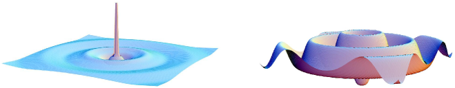
Figure 2: Typical plots of $F_{12}$ for the sinh-Gordon (left) and sine-Gordon (right) cases. The parameters are the same as those in Figs. 1 and 3.

VI.2 Sine-Gordon equation

We finally consider case (ii) of section IV. An axisymmetric solution then satisfies, from eq. (30),

$$\frac{d^{2}\alpha}{dr^{2}}+\frac{1}{r}\frac{d\alpha}{dr}+\frac{\kappa^{2}}{2}\sin(2\alpha)=0.$$ (42)

A change of variables shows that this case is also connected to the Painlevé equation of the third kind. In fact, writing $V(r)=e^{i\alpha(r)}$ turns eq. (42) into

$$\frac{d^{2}V}{dr^{2}}-\frac{1}{V}\left(\frac{dV}{dr}\right)^{2}+\frac{1}{r}\frac{dV}{dr}=\frac{\kappa^{2}}{4}\left(V^{3}-\frac{1}{V}\right).$$ (43)

Equation (42) may be investigated along the same lines as in section VI.1. Once again expanding $\alpha(r)$ for small $r$ leads to an equation similar to eq. (39), namely

$$\alpha(r)\xrightarrow[r\to 0]{}a+\frac{\kappa^{2}}{8}\sin(2a)\,r^{2}+\frac{\kappa^{4}}{256}\sin(4a)\,r^{4}+\mathcal{O}(r^{6}),$$ (44)

which can be used to generate initial conditions for $\alpha(r)$ and $\alpha^{\prime}(r)$ at $r\approx 0$ (we note that exact asymptotic expressions, similar to equations (40) and (41), are also available for this case${}^{\ref{fn1}}$ novo1 ; novo2 ; novo3 ; novo4 ; book ). This, in turn, may be used to numerically integrate eq. (42). Proceeding similarly to the previous case, we start with $\alpha(10^{-3})$ and $\alpha^{\prime}(10^{-3})$ defined by eq. (44), with $\kappa=1$ and $a=\frac{3\pi}{4}$. This yields the plots of Fig. 3. A noticeable difference with the sinh-Gordon case is that the solutions are not localized in any sense here, as shown by the comparison between Figs. 1 and 3. This is further illustrated in Fig. 2, where we compare the Abelian field strength $F_{12}$ obtained for the sinh-Gordon and sine-Gordon cases.

Figure 3: First column: typical plots of $\alpha$ as a function of the radial coordinate $r$ for the sine-Gordon case. Second column: reduced action density $\sigma$ as a function of $r$. Third column: $2\pi\int_{0}^{R}\sigma(r)\,rdr$ as a function of $R$. Fourth column: azimuthal component $J_{\theta}$ of the Abelian current $\mathbf{J}$ for the sine-Gordon case.

VII Smooth solutions in $T^{2}$ for $G=SO(2,1)$

Finally, we remark that the elliptic sinh-Gordon equation eq. (29b) admits smooth doubly-periodic solutions on the 2-torus $T^{2}$. In tcl-prl , the authors show that eq. (29b) appears in problems related to fluid and plasma physics and, in tcl , the same authors construct solutions in closed form in terms of Riemann theta functions. This kind of solutions to eq. (29b), given in terms of $\theta$-functions, are extensively analyzed in B . Evidently, such solutions may in turn be regarded as smooth solutions of the $SO(2,1)$ Hitchin’s equations on the 2-torus $T^{2}=\mathbb{R}^{2}/\mathbb{Z}^{2}$.

To describe the solutions, we must consider a smooth hyperelliptic curve $C\subset\mathbb{C}^{2}$ of genus $g\geq 1$, known as the spectral curve, which is given by:

$$C=\{(u,w)\in\mathbb{C}^{2}~{}|~{}u^{2}=w\cdot\Pi_{k=1}^{g}(w-\lambda_{k})(w-\overline{\lambda_{k}}^{-1})\},$$

where the parameters $\lambda_{1},\dots,\lambda_{g}$ are all distinct and satisfy $|\lambda_{k}|\neq 1$. Now let $\theta:\mathbb{C}^{g}\to\mathbb{C}$ be the Riemann $\theta$-function for the curve $C$ GH . As it is shown by Bobenko B , every doubly-periodic, non-singular, real-valued solution of the elliptic sinh-Gordon equation (29b) is of the form

$$\alpha(z,\overline{z})=2\log\left(\frac{\theta(-i(Uz+V\overline{z})/2+D)}{\theta(-i(Uz+V\overline{z})/2+D+\Delta)}\right)$$ (45)

where $D$ is an arbitrary imaginary vector in $\mathbb{C}^{g}$, $\Delta=i\pi(1,\dots,1)\in\mathbb{C}^{g}$, and $U,V\in\mathbb{C}^{g}$ are the period vectors, which are uniquely determined by the curve $C$.

For a fixed value of $g\geq 1$, notice that the set of doubly-periodic, non-singular, real-valued solutions of (29b) depends on $3g$ real parameters: the $g$ complex parameters $\lambda_{1},\dots,\lambda_{g}$ (which determine the spectral curve $C$ and therefore determines the $\theta$-function and the vectors $U,V$) plus $g$ real parameters determining the imaginary vector $D\in\mathbb{C}^{g}$. We therefore conclude that the moduli space of smooth solutions the $SO(2,1)$ Hitchin’s equations on $T^{2}$ posesses an infinite number of connected components which are parametrized by a positive integer $g\geq 1$ (the genus of the spectral curve), and that each connected component has dimension at least $3g$.

VIII Conclusion

In this paper, we have discussed smooth real solutions of the $SO(2,1)$ Hitchin’s equations on $\mathbb{R}^{2}$, $S^{2}$ and $T^{2}$, even though there are no such solutions for the $SU(2)$ Hitchin’s equations. This was done by using an ansatz that reduced the $SO(2,1)$ Hitchin’s equations to three classical integrable equations.

We believe that our calculations provide a strong motivation for further study of Yang-Mills theory for noncompact real Lie groups. We provided evidence that some of the good properties of Yang-Mills theory for compact real Lie groups, like the possible existence of finite dimensional moduli spaces and the link with integrability, are preserved when noncompact real Lie groups are considered. We propose that a general Yang-Mills theory for complex Lie groups and its noncompact real forms ought to be developed.

- (1) S. K. Donaldson and P. B. Kronheimer, The geometry of four-manifolds, Claredon Press, Oxford (1990).
- (2) H. Nakajima, “Instantons on ALE spaces, quiver varieties, and Kac-Moody algebras”, Duke Math. J. 76, 365-416 (1994).
- (3) N. Hitchin, “Stable bundles and integrable systems”, Duke Math. J. 54, 91-114 (1987).
- (4) L. J. Mason and N. M. J. Woodhouse, Integrability, self-duality, and twistor theory, Clarendon Press, Oxford (1996).
- (5) C. Rebbi, “Self-dual Yang-Mills fields in Minkowski space-time”, Phys. Rev. D 17, 483-485 (1978).
- (6) G. Etesi, “Gravitational interpretation of the Hitchin equations”, J. Geom. Phys. 57, 1778-1788 (2007), math.DG/0605590.
- (7) N. Hitchin, “The self-duality equations on a Riemann surface”, Proc. London Math. Soc. 55, 59-126 (1987).
- (8) C. Saçlıog̃lu, “Liouville and Painlevé equations and Yang-Mills strings”, J. Math. Phys. 25, 3214-3220 (1984).
- (9) S. K. Donaldson, “Twisted harmonic maps and the self-duality equations”, Proc. London Math. Soc. 55, 127-131 (1987).
- (10) L. Bonora, “Yang-Mills theory and matrix string theory”, In Quantum field theory, A. N. Mitra (ed.), pp. 665-699, Hindustan Book Agency, New Delhi (2000).
- (11) J. Liouville, “Sur l’équation aux différences partielles =0”, J. Math. Pure Appl. 18, 71 (1853).
- (12) R. A. Mosna, “Singular solutions to the Seiberg-Witten and Freund equations on flat space from an iterative method”, J. Math. Phys. 47, 013514 (2006), math-ph/0511038.
- (13) E. L. Ince, Ordinary Differential Equations, Dover, New York (1956).
- (14) V. Yu. Novokshenov, “The method of isomonodromic deformation and the asymptotics of the third Painlevé transcendent”, Funct. Anal. Appl. 18, 260-262 (1984).
- (15) V. Yu. Novokshenov, “On the asymptotics of the general real-valued solution to the third Painlevé equation”. Dokl. Akad. Nauk. SSSR, 283, 1161-1165 (1985).
- (16) V. Yu. Novokshenov, “Radial-symmetric solution of the cosh-Laplace equation and the distribution of its singularities”, Russian J. Math. Phys. 5, 211-226 (1997).
- (17) V. Yu. Novokshenov, A. G. Shagalov, “Bound states of the elliptic sine-Gordon equation, Physica D 106, 81-94 (1997).
- (18) A. Fokas, A. Its, A. Kapaev, V. Yu. Novokshenov, Painlevé Transcendents: The Riemann-Hilbert Approach. AMS Mathematical Surveys and Monographs, vol. 128 (2006).
- (19) A. C. Ting, H. H. Chen and Y. C. Lee, “Exact Vortex Solutions of Two-Dimensional G uiding-Center Plasmas”, Phys. Rev. Lett. 53, 1348 1351 (1984).
- (20) A. C. Ting, H. H. Chen and Y. C. Lee, “Exact solutions of a nonlinear boundary value problem: the vortices of the two-dimensional sinh-Poisson equation”, Physica D 26, 37-66 (1987).
- (21) A. I. Bobenko, “All constant mean curvature tori in , and in terms of theta functions”, Math. Ann. 290, 209-245 (1991).
- (22) P. Griffiths and J. Harris, Principles of algebraic geometry. John Wiley & sons, New York (1978).