Absolute Time Derivatives

Abstract

A four dimensional treatment of nonrelativistic space-time gives a natural frame to deal with objective time derivatives. In this framework some well known objective time derivatives of continuum mechanics appear as Lie-derivatives. Their coordinatized forms depends on the tensorial properties of the relevant physical quantities. We calculate the particular forms of objective time derivatives for scalars, vectors, covectors and different second order tensors from the point of view of a rotating observer. The relation of substantial, material and objective time derivatives is treated.

1 Introduction

Objectivity plays a fundamental role in continuum physics. Its usual definition is based on time-dependent Euclidean transformations. Some problems arise from it which mainly concern quantities containing derivatives; they take their origin from the fact that objectivity is defined for three-dimensional vectors but differentiation – with respect to time and space together – results in a four-dimensional covector. Using a four-dimensional setting, we have extended the notion of objectivity [1] which puts the objectivity of material time derivatives into new light.

More closely, $\partial_{0}+\mathbf{v}\cdot\nabla$ is usually considered to be material time derivation. This applied to scalars results in scalars but applied to an objective vector does not result in an objective vector; that is why it is usually stated that this operation is not objective. One of the most important aspects of our four-dimensional treatment is the existence of a covariant derivation in nonrelativistic space-time which results in that the correct form of material time derivation for vectors depends on the observer. For a rotating observer the material time derivative is $\partial_{0}+\mathbf{v}\cdot\nabla+\boldsymbol{\Omega}$ where $\boldsymbol{\Omega}$ is the angular velocity (vorticity) of the observer.

From a mathematical point of view, $\boldsymbol{\Omega}$ is a component of the four-dimensional Christoffel symbols corresponding to the observer. In the usual three-dimensional treatment four-dimensional Christoffel symbols cannot appear. As a consequence, one looks for ‘objective time derivatives’ in such a way that $\partial_{0}+\mathbf{v}\cdot\nabla$ is supplemented by some terms for getting an objective operation which does not involve Christoffel symbols and contains only partial derivatives. This is how one obtains the ‘lower convected time derivative’, the ‘upper convected time derivative’ and the Jaumann or ‘corotational time derivative’, as it is written in several textbooks and monographs of continuum mechanics (e.g. [2, 3, 4]) and especially of rheology (e.g. [5, 6]). The corotational time derivative was first introduced by Jaumann [7], and the convected derivatives by Oldroyd [8].

In the present paper we investigate these derivatives from a four-dimensional point of view. For getting a convenient insight in their physical meaning, we apply a coordinate-free formulation of nonrelativistic space-time.

In the second section we shortly summarize the essentials of the space-time model. In the third section we introduce the observers and space-time splittings on the example of rigid observer. Then continuous media is treated. A four dimensional version of the material manifold is a general observer in our absolute framework. At the fifth section we give the material time derivatives of the physical quantities of different tensorial order. Finally a summary and a discussion of the results follows.

2 Fundamentals of nonrelativistic space-time
model

In this section some notions and results of the nonrelativistic space-time model as a mathematical structure [9, 10] will be recapitulated.

2.1 The structure of nonrelativistic space-time model

A nonrelativistic space-time model consists of

– the space-time $M$ which is a four-dimensional oriented affine space over the vector space $\mathbf{M}$,

– the absolute time $I$ which is a one-dimensional oriented affine space over the vector space $\mathbf{I}$ (measure line of time periods),

– the time evaluation $\tau:M\to I$ which is an affine surjection over the linear map $\boldsymbol{\tau}:\mathbf{M}\to\mathbf{I}$,

– the measure line of distances $\mathbf{D}$ which is a one dimensional oriented vector space,

– the Euclidean structure $\cdot:\mathbf{E}\times\mathbf{E}\to\mathbf{D}\otimes\mathbf{D}$ which is a positive definite symmetric bilinear map where

$$\mathbf{E}:=\mathrm{Ker}\boldsymbol{\tau}\subset\mathbf{M}$$

is the (three-dimensional) linear subspace of spacelike vectors.

The time-lapse between the world points $x$ and $y$ is $\tau(x)-\tau(y)=\boldsymbol{\tau}(x-y)$. Two world points are simultaneous if the time-lapse between them is zero. The difference of two simultaneous world points is a spacelike vector. The essential elements of the model are visualized on figure 1.

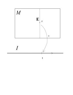
Figure 1: Nonrelativistic space-time model

The length of the spacelike vector $\mathbf{q}$ is $|\mathbf{q}|:=\sqrt{\mathbf{q}\cdot\mathbf{q}}$.

The dual of $\mathbf{M}$, denoted by $\mathbf{M}^{*}$, is the vector space of linear maps $\mathbf{M}\to\mathbb{R}$. Elements of $\mathbf{M}^{*}$ are called covectors.

In a similar way, the dual of $\mathbf{E}$ is $\mathbf{E}^{*}$.

If $\mathbf{K}\in\mathbf{M}^{*}$, i.e. $\mathbf{K}:\mathbf{M}\to\mathbb{R}$ is a linear map, then its restriction to $\mathbf{E}$, is an element of $\mathbf{E}^{*}$, denoted by $\mathbf{K}\cdot\mathbf{i}$ which we call the absolute spacelike component of $\mathbf{K}$.

Note the important fact that the Euclidean structure allows us the identification $\mathbf{E}^{*}\equiv\frac{\mathbf{E}}{\mathbf{D}\otimes\mathbf{D}}$. On the other hand, no similar identification is possible for $\mathbf{M}^{*}$ because there is no Euclidean or pseudo-Euclidean structure in $\mathbf{M}$. (In coordinates: an element $\mathbf{q}$ of $\mathbf{E}$ is coordinatized as $q^{i}$ for $i=1,2,3$ and $q_{i}=q^{i}$ can be written. On the other hand, an element $\mathbf{x}$ of $\mathbf{M}$, $\mathbf{x}\notin\mathbf{E}$ is coordinatized as $x^{\alpha}$ for $\alpha=0,1,2,3$ and $x_{\alpha}$ is not meaningful. Moreover, an element $\mathbf{K}$ of $\mathbf{M}^{*}$ is coordinatized as $K_{\alpha}$ for $\alpha=0,1,2,3$ and $K^{\alpha}=K_{\alpha}$ can be written for $\alpha=1,2,3$ but $K^{0}$ is not meaningful.)

These features of vectors and covectors are consequences of the fact that time is not embedded in space-time. This property of the model eliminates such unphysical possibilities as the ”angle” of space and time. As a result the careful distinction of space-time vectors and covectors is essential: there is no canonical way to identify them.

2.2 Differentiation

The affine structure of space-time implies the existence of an absolute differentiation (in the language of manifolds: a distinguished covariant differentiation).

If $V$ is a finite dimensional affine space over the vector space $\mathbf{V}$, then a map $A:M\to V$ is differentiable at $x$ if there is a linear map $(\mathrm{D}A)(x):\mathbf{M}\to\mathbf{V}$ – the derivative of $A$ at $x$ – such that

$$\lim_{y\to x}\frac{A(y)-A(x)-(\mathrm{D}A)(x)(y-x)}{||y-x||}=0$$

where $||\ \ ||$ is an arbitrary norm on $\mathbf{M}$ (all norms on the finite dimensional vector space $\mathbf{M}$ are equivalent).

As a consequence of the structure of our space-time model, the partial time derivative of $A:M\to V$ makes no sense. On the other hand, the spacelike derivative of $A$ is meaningful because the spacelike vectors form a linear subspace in $\mathbf{M}$: $(\nabla A)(x)$ is the derivative of the function $\mathbf{E}\to V$, $\mathbf{q}\mapsto A(x+\mathbf{q})$ at zero. It is evident then that $(\nabla A)(x)$ is the restriction of the linear map $(\mathrm{D}A)(x)$ onto $\mathbf{E}$. The transpose of a linear map $\mathbf{A}:\mathbf{M}\to\mathbf{V}$ is the linear map $\mathbf{A}^{*}:\mathbf{V}^{*}\to\mathbf{M}^{*}$ defined by $\mathbf{A}^{*}\mathbf{w}:=\mathbf{w}\circ\mathbf{A}$ for $\mathbf{w}\in\mathbf{V}^{*}$. Then, using the customary identification of linear maps as tensors, we can consider

$$\mathrm{D}A(x)\in\mathbf{V}\otimes\mathbf{M}^{*},\qquad(\mathrm{D}A)^{*}(x)\in\mathbf{M}^{*}\otimes\mathbf{V}$$

and

$$\mathbf{x}\cdot(\mathrm{D}A)^{*}(x):=\mathrm{D}A(x)\mathbf{x}\in\mathbf{V},\qquad(\mathrm{D}A)^{*}(x)\mathbf{w}\in\mathbf{M}^{*}$$

for $\mathbf{x}\in\mathbf{M}$ and $\mathbf{w}\in\mathbf{V}^{*}$.

Accordingly,

$$(\nabla A)(x)\in\mathbf{V}\otimes\mathbf{E}^{*},\qquad(\nabla A)^{*}(x)\in\mathbf{E}^{*}\otimes\mathbf{V},$$ (1)

$$\mathbf{q}\cdot(\nabla A)^{*}(x):=(\nabla A)(x)\mathbf{q}\in\mathbf{V},\qquad(\nabla A)^{*}(x)\mathbf{w}\in\mathbf{E}^{*}$$

for $\mathbf{q}\in\mathbf{E}$ and $\mathbf{w}\in\mathbf{V}^{*}$.

In particular,

• the derivative of a scalar field $f:M\to\mathbb{R}$ is a covector field, $\mathrm{D}f(x)\in\mathbf{M}^{*}$,

  $\bullet$  its spacelike derivative is a spacelike covector field, $\nabla f(x)\in\mathbf{E}^{*}$;

• the derivative of a vector field $\mathbf{C}:M\to\mathbf{M}$ is a mixed tensor field, $(\mathrm{D}\mathbf{C})(x)\in\mathbf{M}\otimes\mathbf{M}^{*}$ whose transpose is $(\mathrm{D}\mathbf{C})^{*}(x)\in\mathbf{M}^{*}\otimes\mathbf{M}$,

  $\bullet$  its spacelike derivative is a mixed tensor field, $(\nabla\mathbf{C})(x)\in\mathbf{M}\otimes\mathbf{E}^{*}$ whose transpose is $(\nabla\mathbf{C})^{*}(x)\in\mathbf{E}^{*}\otimes\mathbf{M}$,

• the spacelike derivative of a spacelike vector field $\mathbf{c}:M\to\mathbf{E}$ is a mixed spacelike tensor field, $(\nabla\mathbf{c})(x)\in\mathbf{E}\otimes\mathbf{E}^{*}$ whose transpose is $(\nabla\mathbf{c})^{*}(x)\in\mathbf{E}^{*}\otimes\mathbf{E}$.

• the derivative of a covector field $\mathbf{K}:M\to\mathbf{M}^{*}$ is a cotensor field, $(\mathrm{D}\mathbf{K})(x)\in\mathbf{M}^{*}\otimes\mathbf{M}^{*}$ whose transpose is $(\mathrm{D}\mathbf{K})^{*}(x)\in\mathbf{M}^{*}\otimes\mathbf{M}^{*}$.

Note that both the derivative of a covector field and its transpose are in $\mathbf{M}^{*}\otimes\mathbf{M}^{*}$. Thus, we can define the antisymmetric derivative of $\mathbf{K}$,

$$(\mathrm{D}\land\mathbf{K})(x):=(\mathrm{D}\mathbf{K})^{*}(x)-(\mathrm{D}\mathbf{K})(x).$$

On the contrary, the antisymmetric derivative of a vector field $\mathbf{C}:M\to\mathbf{M}$, in general, does not make sense. The antisymmetric spacelike derivative of a spacelike vector field $\mathbf{c}:M\to\mathbf{E}^{*}$, however, can be defined because the identification $\mathbf{E}^{*}\equiv\frac{\mathbf{E}}{\mathbf{D}\otimes\mathbf{D}}$ implies $\mathbf{E}\otimes\mathbf{E}^{*}\equiv\mathbf{E}^{*}\otimes\mathbf{E}$, so we can put

$$(\nabla\land\mathbf{c})(x):=(\nabla\mathbf{c})^{*}(x)-(\nabla\mathbf{c})(x).$$

3 Observers

3.1 Absolute velocity

The history of a classical masspoint is described by a world line function, a twice continuously differentiable function $r:I\to M$ such that $\tau(r(t))=t$ for all $t\in I$. A world line is the range of a world line function; a world line is a curve in $M$.

If $r$ is a world line function, then $\boldsymbol{\tau}(\dot{r}(t))=1$. That is why we call the elements of the set

$$V(1):=\left\{\mathbf{u}\in\frac{\mathbf{M}}{\mathbf{I}}\biggm{|}\boldsymbol{\tau}(\mathbf{u})=1\right\}$$

absolute velocities. $V(1)$ is a three dimensional affine space over $\frac{\mathbf{E}}{\mathbf{I}}$.

3.2 Rigid observers

An observer, from a physical point of view, is a ‘continuous set of material points’. Such a ‘continuous body’ can be characterized by assigning to any world point the absolute velocity of the particle at that point, i.e. by an absolute velocity field. Thus we accept that an observer is a smooth map

$$\mathbf{U}:M\to V(1).$$

The integral curves of $\mathbf{U}$ are world lines, representing the histories of the material points that the observer is constituted of. Thus it is quite evident that a maximal integral curve of $\mathbf{U}$ is a space point of the observer. The set of the maximal integral curves is the space of the observer, briefly the $\mathbf{U}$-space.

Keep in mind the most important – but trivial – fact concerning observers: a space point of an observer is a curve in space-time.

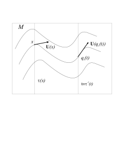
Figure 2: Observers and observer spaces

Observers and their spaces are well defined simple and straightforward notions. The spaces of different observers are evidently different.

For an observer $\mathbf{U}$, we denote by $q_{x}$ the world line function whose range is the $\mathbf{U}$-space point containing the world point $x$, i.e.

$$\frac{\mathrm{d}q_{x}(t)}{\mathrm{d}t}=\mathbf{U}(q_{x}(t)),\qquad q_{x}(\tau(x))=x.$$

$\mathbf{U}$ is rigid if the distance of any two of its space points is time independent: given $x,y$ arbitrarily, then $|q_{x}(t)-q_{y}(t)|=|q_{x}(s)-q_{y}(s)|$ for all instants $t,s$.

It can be shown ([10], Chapter I.4) that the observer $\mathbf{U}$ is rigid if and only if for all $t,t_{\mathrm{o}}\in I$ there is a rotation $\mathbf{R}(t,t_{\mathrm{o}})$ in $\mathbf{E}$ such that

$$q_{x_{\mathrm{o}}+\mathbf{q}}(t)-q_{x_{\mathrm{o}}}(t)=\mathbf{R}(t,t_{\mathrm{o}})\mathbf{q}\qquad(\tau(x_{\mathrm{o}})=t_{\mathrm{o}},\mathbf{q}\in\mathbf{E}).$$ (2)

Then putting $\dot{\mathbf{R}}(t,t_{\mathrm{o}}):=\frac{\partial\mathbf{R}(t,t_{\mathrm{o}})}{\partial t}$,

$$\boldsymbol{\Omega}(t):=\dot{\mathbf{R}}(t,t_{\mathrm{o}})\mathbf{R}(t,t_{\mathrm{o}})^{-1}\in\frac{\mathbf{E}\otimes\mathbf{E}^{*}}{\mathbf{I}}$$

is independent of $t_{\mathrm{o}}$; it is the angular velocity of the rigid observer at the instant $t$. It is easy to show that $\boldsymbol{\Omega}(t)$ is antisymmetric, moreover,

$$\mathbf{U}(x+\mathbf{q})-\mathbf{U}(x)=\boldsymbol{\Omega}(\tau(x))\mathbf{q}\qquad(x\in M,\mathbf{q}\in\mathbf{E}),$$ (3)

which implies that $\nabla\mathbf{U}(x)=\boldsymbol{\Omega}(\tau(x))$: the spacelike derivative of the rigid observer is its angular velocity which is a spacelike antisymmetric tensor.

Since the spacelike derivative of $\mathbf{U}$ is antisymmetric, we have $\nabla\mathbf{U}(x)=-\frac{1}{2}(\nabla\land\mathbf{U})(x)$. This supports that later (20) is considered as the angular velocity of an arbitrary (non-necessarily rigid) continuum.

An important particular rigid observer is the inertial observer, when

$$\mathbf{U}(x)=\text{const}.$$

therefore $\mathbf{R}$ is the identity of $\mathbf{E}$ and $\nabla\mathbf{U}(x)={\bf 0}$.

3.3 Splitting of space-time by rigid observers

Let us consider an observer $\mathbf{U}$. For every world point $x$ there is a unique $\mathbf{U}$-space point (world line, representing a point of the observer) containing $x$ (the range of the world line function $q_{x}$). Accordingly, the observer perceives the world point $x$ as a couple of its absolute instant $\tau(x)$ and the corresponding $\mathbf{U}$-space point. We say that the observer splits space-time into the Cartesian product of time and $\mathbf{U}$-space.

Since $\mathbf{U}$-space is not a simple mathematical object, in general, the splitting of space-time by $\mathbf{U}$ is not simple either. To overcome this uneasiness, we consider vectorized splittings in which $\mathbf{U}$-space is represented by $\mathbf{E}$ as follows.

Let $\mathbf{U}$ be a rigid observer and let $o$ be a world point, conceived as a chosen ‘origin’ in space-time. Then a space point of the observer will be represented by the spacelike vector which is the difference between $o$ and the simultaneous world point of the space point in question. More closely, the $\mathbf{U}$-space point (world line) containing the world point $x$ will be represented by $q_{x}(\tau(o))-o$. To get explicitly how $q_{x}(\tau(o))-o$ depends on $x$, let us put $x_{\mathrm{o}}:=o$, $\mathbf{q}:=q_{x}(\tau(o))-o$ and $t=\tau(x)$ in (2) (then $\tau(o)=t_{\mathrm{o}}$) and take into account that $q_{q_{x}(t_{\mathrm{o}})}(\tau(x))=x$; in this way we obtain the vectorized splitting in the form

$$H:M\to I\times\mathbf{E},\quad x\mapsto\bigl{(}\tau(x),\mathbf{R}(\tau(x))^{-1}\bigl{(}x-q_{o}(\tau(x))\bigr{)}.$$ (4)

Here and in the sequel, for the sake of brevity, $\mathbf{R}(t):=\mathbf{R}(t,t_{\mathrm{o}})$.

Figure 3: Splitting of space-time

The observer splits $\mathbf{M}$, too, by the derivative of this space-time splitting.

Differentiating $\mathbf{R}(\tau(x))^{-1}$ by $x$ we get $-\mathbf{R}(\tau(x))^{-1}\dot{\mathbf{R}}(\tau(x))\mathbf{R}(\tau(x))^{-1}\boldsymbol{\tau}$, taking into account $\dot{q}_{o}(\tau(x))=\mathbf{U}(q_{o}(\tau(x))$ and the basic properties of world line functions we find that the vectorized splitting has the derivative

$$\mathrm{D}H(x)=\begin{pmatrix}\boldsymbol{\tau}\\ \mathbf{R}(\tau(x))^{-1}\left(\boldsymbol{1}-\mathbf{U}(x)\otimes\boldsymbol{\tau}\right)\end{pmatrix}:\mathbf{M}\to\mathbf{I}\times\mathbf{E}$$ (5)

where $\boldsymbol{1}$ is the identity of $\mathbf{M}$.

Note that restricting $\mathrm{D}H(x)$ onto $\mathbf{E}$, we obtain $\nabla H(x)=(0,\mathbf{R}(\tau(x))^{-1})$; further we omit the zero component, thus we consider that

$$\nabla H(x)=\mathbf{R}(\tau(x))^{-1}:\mathbf{E}\to\mathbf{E}.$$

The inverse of the splitting is

$$H^{-1}=:P:I\times\mathbf{E}\to M,\quad(t,\mathbf{q})\mapsto q_{o}(t)+\mathbf{R}(t)\mathbf{q},$$ (6)

whose partial derivatives are obtained easily:

$$\partial_{0}P(t,\mathbf{q}):=\frac{\partial P(t,\mathbf{q})}{\partial t}=\mathbf{U}(q_{o}(t))+\dot{\mathbf{R}}(t)\mathbf{q}=\mathbf{U}(P(t,\mathbf{q})),$$ (7)

$$\boldsymbol{\nabla}P(t,\mathbf{q}):=\frac{\partial P(t,\mathbf{q})}{\partial\mathbf{q}}=\mathbf{R}(t).$$ (8)

The derivative of $P$ is the couple of the partial derivatives. Differentiating the equality $H(P(t,\mathbf{q}))=(t,\mathbf{q})$, we deduce

$$\biggl{(}\partial_{0}P,\boldsymbol{\nabla}P\biggr{)}=(\mathrm{D}H(P))^{-1}.$$ (9)

3.4 Relative form of absolute physical quantities

Using the splitting of $M$ and $\mathbf{M}$, a rigid observer $\mathbf{U}$ represents physical quantities – functions defined in space-time – as functions defined in time and $\mathbf{U}$-space. The splitting of the space-time functions gives their $\mathbf{U}$-relative form, the usual field quantities defined on time and space.

The $\mathbf{U}$-relative form of a scalar field $f:M\to\mathbb{R}$ is

$$f_{{}_{\mathbf{U}}}:I\times\mathbf{E}\to\mathbb{R},\quad(t,\mathbf{q})\mapsto f(P(t,\mathbf{q})),$$ (10)

briefly: $f_{{}_{\mathbf{U}}}=f(P)$.

The $\mathbf{U}$-relative form of a vector field $\mathbf{C}:M\to\mathbf{M}$ is

$$\mathbf{C}_{{}_{\mathbf{U}}}:I\times\mathbf{E}\to\mathbf{I}\times\mathbf{E},\quad(t,\mathbf{q})\mapsto\mathrm{D}H(P(t,\mathbf{q}))\mathbf{C}(P(t,\mathbf{q})).$$

Using (5) and an abbreviated notation, we have

$$\mathbf{C}_{{}_{\mathbf{U}}}=\begin{pmatrix}\boldsymbol{\tau}\mathbf{C}(P)\\ \mathbf{R}^{-1}\bigl{(}\mathbf{C}(P)-\mathbf{U}(P)\boldsymbol{\tau}\mathbf{C}(P)\bigr{)}\end{pmatrix}$$ (11)

In particular, a spacelike vector field $\mathbf{c}:M\to\mathbf{E}$ has the $\mathbf{U}$-relative form (the trivial zero component omitted)

$$\mathbf{c}_{{}_{\mathbf{U}}}=\mathbf{R}^{-1}\mathbf{c}(P).$$ (12)

Similarly, a spacelike tensor field $\mathbf{f}:M\to\mathbf{E}\otimes\mathbf{E}^{*}$ has the $\mathbf{U}$-relative form

$$\mathbf{f}_{{}_{\mathbf{U}}}=\mathbf{R}^{-1}\mathbf{f}(P)\mathbf{R}.$$ (13)

The $\mathbf{U}$-relative form of a covector field $\mathbf{K}:M\to\mathbf{M}^{*}$ is

$$\mathbf{K}_{{}_{\mathbf{U}}}:=\left((\mathrm{D}H(P))^{-1}\right)^{*}\mathbf{K}(P)=\mathbf{K}(P)(\mathrm{D}H(P))^{-1}:I\times\mathbf{E}\to\mathbf{I}^{*}\times\mathbf{E}^{*};$$

by (9), (7) and (8), we find

$$\mathbf{K}_{{}_{\mathbf{U}}}=\mathbf{K}(P)\cdot\biggl{(}\partial_{0}P,\boldsymbol{\nabla}P\biggr{)}=\biggl{(}\mathbf{K}(P)\cdot\mathbf{U}(P),(\mathbf{K}(P)\cdot\mathbf{i})\mathbf{R}\biggr{)}$$ (14)

(recall that $\mathbf{K}\cdot\mathbf{i}$ denotes the absolute spacelike component of $\mathbf{K}$, the restriction of $\mathbf{K}$ onto $\mathbf{E}$). Note that the spacelike component can be written in the form $\mathbf{R}^{-1}(\mathbf{K}(P)\cdot\mathbf{i})$, too, because for an orthogonal map we have $\mathbf{R}^{*}=\mathbf{R}^{-1}$.

As a consequence one may calculate the $\mathbf{U}$-relative form of second order tensors easily. For example, a mixed tensor field $\mathbf{F}:M\to\mathbf{E}\otimes\mathbf{M}^{*}$ has the $\mathbf{U}$-relative form

$$\mathbf{F}_{{}_{\mathbf{U}}}=\biggl{(}\mathbf{R}^{-1}\mathbf{F}(P)\cdot\mathbf{U}(P),\mathbf{R}^{-1}(\mathbf{F}(P)\cdot\mathbf{i})\mathbf{R}\biggr{)}.$$ (15)

3.5 Relative form of absolute derivatives

The derivative $\mathrm{D}f$ of a scalar field $f$ is a covector field, thus its $\mathbf{U}$-relative form is

$$(\mathrm{D}f)_{{}_{\mathbf{U}}}=\mathrm{D}f(P)\cdot\biggl{(}\partial_{0}P,\boldsymbol{\nabla}P\biggr{)}=\biggl{(}\partial_{0}f_{{}_{\mathbf{U}}},\boldsymbol{\nabla}f_{{}_{\mathbf{U}}}\biggr{)}.$$ (16)

The derivative $\mathrm{D}\mathbf{c}$ of a spacelike vector field $\mathbf{c}$ is a mixed tensor field, so differentiating (12) and applying (15), we get

$$(\mathrm{D}\mathbf{c})_{{}_{\mathbf{U}}}=\biggl{(}(\partial_{0}+\boldsymbol{\Omega}_{{}_{\mathbf{U}}})\mathbf{c}_{{}_{\mathbf{U}}},\boldsymbol{\nabla}\mathbf{c}_{{}_{\mathbf{U}}}\biggr{)}$$ (17)

where

$$\boldsymbol{\Omega}_{{}_{\mathbf{U}}}:=\mathbf{R}^{-1}\boldsymbol{\Omega}\mathbf{R}=\mathbf{R}^{-1}\dot{\mathbf{R}}$$ (18)

is the relative form of the angular velocity of the observer.

As a consequence,

$$(\nabla\mathbf{c})_{{}_{\mathbf{U}}}=\boldsymbol{\nabla}\mathbf{c}_{{}_{\mathbf{U}}}.$$ (19)

4 Continuous media

A continuum, from a physical point of view, is a ‘continuous set of material points’. The history of such a ‘continuous body’ can be described by an absolute velocity field $\mathbf{u}:M\to V(1)$ which is supposed to be twice differentiable.

Note that both an observer and a continuum are given by an absolute velocity field. Keep in mind that majuscule $\mathbf{U}$ will refer to an observer (an ‘observing body’), minuscule $\mathbf{u}$ will refer to a continuum (a ‘body to be observed’). An observer is mostly supposed to be rigid, a continuum is never rigid. An observer has no other property besides its velocity field, a continuum has other characteristics, too: density, stress, temperature, etc.

4.1 Velocity fields

Recall that $V(1)$ is an affine space over $\frac{\mathbf{E}}{\mathbf{I}}$, thus

• the derivative of an absolute velocity field $\mathbf{u}:M\to V(1)$ is a mixed tensor field, $(\mathrm{D}\mathbf{u})(x)\in\frac{\mathbf{E}}{\mathbf{I}}\otimes\mathbf{M}^{*}$ having the transpose $(\mathrm{D}\mathbf{u})^{*}(x)\in\mathbf{M}^{*}\otimes\frac{\mathbf{E}}{\mathbf{I}}$.

• the spacelike derivative of $\mathbf{u}$ is a mixed spacelike tensor field, $(\nabla\mathbf{u})(x)\in\frac{\mathbf{E}}{\mathbf{I}}\otimes\mathbf{E}^{*}$ having the transpose $(\nabla\mathbf{u})^{*}(x)\in\mathbf{E}^{*}\otimes\frac{\mathbf{E}}{\mathbf{I}}$.

In view of the identification $\mathbf{E}^{*}\equiv\frac{\mathbf{E}}{\mathbf{D}\otimes\mathbf{D}}$, both $(\nabla\mathbf{u})(x)$ and $(\nabla\mathbf{u})^{*}(x)$ are considered to be in $\frac{\mathbf{E}\otimes\mathbf{E}}{\mathbf{I}\otimes\mathbf{D}\otimes\mathbf{D}}$, thus the antisymmetric spacelike derivative of $\mathbf{u}$ makes sense, too:

$$(\nabla\land\mathbf{u})(x):=(\nabla\mathbf{u})^{*}(x)-(\nabla\mathbf{u})(x).$$

According to the end of Subsection 3.2, we can interpret

$$-\frac{1}{2}(\nabla\land\mathbf{u})(x)$$ (20)

as the angular velocity (vorticity) of the continuum at the world point $x$.

Now let us consider a rigid observer $\mathbf{U}$ which ‘observes’ the continuum $\mathbf{u}$. We deduce from (11) that the $\mathbf{U}$-relative form of $\mathbf{u}$ is

$$\mathbf{u}_{{}_{\mathbf{U}}}(t,\mathbf{q})=\begin{pmatrix}1\\ \mathbf{v}_{{}_{\mathbf{U}}}(t,\mathbf{q})\end{pmatrix}$$ (21)

where

$$\mathbf{v}_{{}_{\mathbf{U}}}=\mathbf{R}^{-1}\bigl{(}\mathbf{u}(P)-\mathbf{U}(P)\bigr{)}$$ (22)

is the $\mathbf{U}$-relative velocity field.

Then we derive that

$$\boldsymbol{\nabla}\mathbf{v}_{{}_{\mathbf{U}}}=\mathbf{R}^{-1}\bigl{(}(\nabla\mathbf{u})(P)\boldsymbol{\nabla}P-(\nabla\mathbf{U})(P)\boldsymbol{\nabla}P\bigr{)}$$ (23)

from which, taking into account that $\nabla\mathbf{u}$ is a spacelike tensor and using (8) and (13), we have

$$(\nabla\mathbf{u})_{{}_{\mathbf{U}}}=\boldsymbol{\nabla}\mathbf{v}_{{}_{\mathbf{U}}}+\boldsymbol{\Omega}_{{}_{\mathbf{U}}}\quad\mbox{or}\quad(\nabla\mathbf{u})^{*}_{{}_{\mathbf{U}}}=(\boldsymbol{\nabla}\mathbf{v}_{{}_{\mathbf{U}}})^{*}-\boldsymbol{\Omega}_{{}_{\mathbf{U}}}.$$ (24)

4.2 The flow of a continuum

A velocity field $\mathbf{u}$, by the solution of differential equation $\dot{x}=\mathbf{u}(x)$, generates a flow, the map

$$\mathbf{I}\times M\to M,\quad(\mathbf{t},x)\mapsto\Upsilon_{\mathbf{t}}(x)$$

such that

$$\frac{\mathrm{d}\Upsilon_{\mathbf{t}}(x)}{\mathrm{d}\mathbf{t}}=\mathbf{u}(\Upsilon_{\mathbf{t}}(x)),\qquad\Upsilon_{0}(x)=x.$$ (25)

Thus, $t\mapsto\Upsilon_{t-\tau(x)}(x)$ is a world line function of $\mathbf{u}$, describing the history of a particle of the continuum.

It is well known from the theory of differential equations [11] that for any fixed $\mathbf{t}$ the map $M\to M$, $x\mapsto\Upsilon_{\mathbf{t}}(x)$ is a twice differentiable bijection whose inverse is twice differentiable, too (it is a diffeomorphism). Consequently, its derivative $\mathrm{D}\Upsilon_{\mathbf{t}}(x):=\frac{\mathrm{d}\Upsilon_{\mathbf{t}}(x)}{\mathrm{d}x}$ is a linear bijection $\mathbf{M}\to\mathbf{M}$ (an element of $\mathbf{M}\otimes\mathbf{M}^{*}$). Note that $\mathrm{D}\Upsilon_{0}(x)$ is the identity of $\mathbf{M}$.

The order of differentiations can be interchanged, thus

$$\frac{\mathrm{d}\mathrm{D}\Upsilon_{\mathbf{t}}(x)}{\mathrm{d}\mathbf{t}}\left.\right|_{\mathbf{t}=0}=\mathrm{D}\mathbf{u}(x).$$ (26)

The customary notions regarding the kinematics of the continuum are connected to the U-relative form of the flow. According to the previous general case a rigid observer splits the flow of the continuum into the duration t of the motion, the time elapsed from the initial instant, and the motion function $\chi_{\mathbf{t}}$ [12], the relative position of the particles of the continuum in the space of the rigid observer:

$$(\Upsilon_{\mathbf{t}})_{{}_{\mathbf{U}}}:I\times\mathbf{E}\to\mathbf{I}\times\mathbf{E},\quad(t,\mathbf{X})\mapsto DH(P(t,\mathbf{X}))\Upsilon_{\mathbf{t}}(P(t,\mathbf{X})).$$

With the customary and shortened notation one can get

$$(\Upsilon_{\mathbf{t}})_{{}_{\mathbf{U}}}(t,\mathbf{X})=(\boldsymbol{\tau}(\Upsilon_{\mathbf{t}}),\mathbf{R}^{-1}(\Upsilon_{\mathbf{t}}-\mathbf{U}\boldsymbol{\tau}(\Upsilon_{\mathbf{t}})))=:(\mathbf{t},\chi_{\mathbf{t}}(\mathbf{X})).$$

The spacelike part of the domain of the $\mathbf{U}$-relative flow is called reference configuration, because $\chi_{\bf 0}(\mathbf{X})=\mathbf{X}$ as a consequence of the second formula of (25). Let us note that the spacelike component of the flow, the motion function, is a relative notion, depends on the observer [13]. Similarly, the usual concepts of body and material manifold of continuum physics (see e.g. [12, 14]) are relative, too.

5 Time derivatives

In this section we consider a continuum having the absolute velocity field $\mathbf{u}$.

5.1 Material time derivative

Let a physical quantity be described by $A:M\to V$ where $V$ is a finite dimensional affine space. The function $\mathbf{t}\mapsto A(\Upsilon_{\mathbf{t}}(x))$ is the change in time of the quantity along an integral curve i.e. at a particle of the continuum. We have by the chain rule that

$$\frac{\mathrm{d}A(\Upsilon_{\mathbf{t}}(x))}{\mathrm{d}\mathbf{t}}\left.\right|_{\mathbf{t}=0}=\mathrm{D}A(x)\cdot\mathbf{u}(x)=\mathbf{u}(x)\cdot(\mathrm{D}A)^{*}(x)=:(\mathrm{D}_{\mathbf{u}}A)(x).$$

It is a matter of course that we call $\mathrm{D}_{\mathbf{u}}A=(\mathrm{D}A)\cdot\mathbf{u}$ the material time derivative of $A$ with respect to $\mathbf{u}$. Clearly, this is an absolute object, not depending on any observer.

The $\mathbf{U}$-relative form of the material time derivative of a scalar field $f:M\to\mathbb{R}$ is obtained by (16) and (21):

$$(\mathrm{D}_{\mathbf{u}}f)_{{}_{\mathbf{U}}}= (\mathrm{D}f\cdot\mathbf{u})_{{}_{\mathbf{U}}}=(\mathrm{D}f)_{{}_{\mathbf{U}}}\cdot(\mathbf{u})_{{}_{\mathbf{U}}}=$$

$$= (\partial_{0}+\mathbf{v}_{{}_{\mathbf{U}}}\cdot\boldsymbol{\nabla})f_{{}_{\mathbf{U}}}.$$

The $\mathbf{U}$-relative form of the material time derivative of a spacelike vector field $\mathbf{c}:M\to\mathbf{E}$ is obtained by (17) and (21):

$$(\mathrm{D}_{\mathbf{u}}\mathbf{c})_{{}_{\mathbf{U}}}= \bigl{(}\mathrm{D}\mathbf{c}\cdot\mathbf{u}\bigr{)}_{{}_{\mathbf{U}}}=(\mathrm{D}\mathbf{c})_{{}_{\mathbf{U}}}\cdot(\mathbf{u})_{{}_{\mathbf{U}}}=$$

$$= \left(\partial_{0}+\boldsymbol{\Omega}_{{}_{\mathbf{U}}}+\mathbf{v}_{{}_{\mathbf{U}}}\cdot\boldsymbol{\nabla}\right)\mathbf{c}_{{}_{\mathbf{U}}}.$$ (27)

We emphasize that material time differentiation is absolute (objective), does not depend on any observer and its correct relative form by a rigid observer for absolute spacelike vector fields is $\partial_{0}+\boldsymbol{\Omega}_{{}_{\mathbf{U}}}+\mathbf{v}_{{}_{\mathbf{U}}}\cdot\boldsymbol{\nabla}$. We repeat for a clear distinction: the non-objective $\partial_{0}+\mathbf{v}_{{}_{\mathbf{U}}}\cdot\boldsymbol{\nabla}$ is not the relative form of the material time differentiation for spacelike vector fields [1].

5.2 Traditional convected time derivatives

5.2.1 Upper convected time derivative

Now we have to make a remark. Let $N$ be an affine space and let $H:M\to N$ be a diffeomorphism. Then the vector field $\mathbf{C}:M\to\mathbf{M}$ is sent by $H$ to the vector field $N\to\mathbf{N}$, $y\mapsto\mathrm{D}H(y)\mathbf{C}(H^{-1}(y))$. This formula is applied when defining the split form (11) of a vector field and offers itself for the flow generated by the velocity field, $H$ replaced with $\Upsilon_{\mathbf{t}}^{-1}$.

Figure 4: Pull-back of a vector to the material manifold

Thus, instead of $t\mapsto\mathbf{C}(\Upsilon_{\mathbf{t}}(x))$, it seems preferable to consider
$\mathbf{t}\mapsto(\mathrm{D}\Upsilon_{\mathbf{t}}(x))^{-1}\mathbf{C}(\Upsilon_{\mathbf{t}}(x))$ as the change in time of the vector field along a particle of the continuum. Since

$$\frac{\mathrm{d}(\mathrm{D}\Upsilon_{\mathbf{t}}(x))^{-1}}{\mathrm{d}\mathbf{t}}=-(\mathrm{D}\Upsilon_{\mathbf{t}}(x))^{-1}\frac{\mathrm{d}\mathrm{D}\Upsilon_{\mathbf{t}}(x)}{\mathrm{d}\mathbf{t}}(\mathrm{D}\Upsilon_{\mathbf{t}}(x))^{-1},$$

so

$$\left.\frac{\mathrm{d}(\mathrm{D}\Upsilon_{\mathbf{t}}(x))^{-1}\mathbf{C}(\Upsilon_{\mathbf{t}}(x))}{\mathrm{d}\mathbf{t}}\right|_{\mathbf{t}=0}=\mathbf{u}(x)\cdot(\mathrm{D}\mathbf{C})^{*}(x)-\mathbf{C}(x)\cdot(\mathrm{D}\mathbf{u})^{*}(x)=:(L_{\mathbf{u}}\mathbf{C})(x).$$ (28)

We mention that $L_{\mathbf{u}}\mathbf{C}$ is known in differential geometry as the Lie derivative of $\mathbf{C}$ by $\mathbf{u}$ [15].

The first term of the Lie derivative is just the material time derivative.

For a spacelike vector field $\mathbf{c}:M\to\mathbf{E}$ we have

$$L_{\mathbf{u}}\mathbf{c}=\mathrm{D}_{\mathbf{u}}\mathbf{c}-\mathbf{c}\cdot(\nabla\mathbf{u})^{*}.$$ (29)

The $\mathbf{U}$-relative form of the Lie derivative of the spacelike vector field $\mathbf{c}$ is

$$(L_{\mathbf{u}}\mathbf{c})_{{}_{\mathbf{U}}}= (\partial_{0}+\boldsymbol{\Omega}_{{}_{\mathbf{U}}}+\mathbf{v}_{{}_{\mathbf{U}}}\cdot\boldsymbol{\nabla})\mathbf{c}_{{}_{\mathbf{U}}}-\mathbf{c}_{{}_{\mathbf{U}}}\cdot((\boldsymbol{\nabla}\mathbf{v}_{{}_{\mathbf{U}}})^{*}-\boldsymbol{\Omega}_{{}_{\mathbf{U}}})=$$

$$= (\partial_{0}+\mathbf{v}_{{}_{\mathbf{U}}}\cdot\boldsymbol{\nabla})\mathbf{c}_{{}_{\mathbf{U}}}-\mathbf{c}_{{}_{\mathbf{U}}}\cdot(\boldsymbol{\nabla}\mathbf{v}_{{}_{\mathbf{U}}})^{*}$$ (30)

which is exactly the known form of the upper convected time derivative.

Thus, the upper convected time derivative of a spacelike vector field is just its Lie derivative by the velocity field of the continuum.

5.2.2 Lower convected time derivatives

An argument similar to that in the previous Subsection yields that, instead of $\mathbf{t}\mapsto\mathbf{K}(\Upsilon_{\mathbf{t}}(x))$, it seems preferable to consider $\mathbf{t}\mapsto(\mathrm{D}\Upsilon_{\mathbf{t}}(x))^{*}\mathbf{K}(\Upsilon_{\mathbf{t}}(x))$ as the change in time of the covector field $\mathbf{K}:M\to\mathbf{M}^{*}$ along a particle of the continuum. Then we find

$$\left.\frac{\mathrm{d}(\mathrm{D}\Upsilon_{\mathbf{t}}(x))^{*}\mathbf{K}(\Upsilon_{\mathbf{t}}(x))}{\mathrm{d}\mathbf{t}}\right|_{\mathbf{t}=0}=\mathbf{u}(x)(\mathrm{D}\mathbf{K})^{*}(x)+(\mathrm{D}\mathbf{u})^{*}(x)\mathbf{K}(x)=:(L_{\mathbf{u}}\mathbf{K})(x)$$ (31)

We mention that $L_{\mathbf{u}}\mathbf{K}$ is known in differential geometry as the Lie derivative of $\mathbf{K}$ by $\mathbf{u}$.

The first term of the Lie derivative is just the material time derivative.

Recall that $(\mathrm{D}\mathbf{u})^{*}(x)$ is in $\mathbf{M}^{*}\otimes\frac{\mathbf{E}}{\mathbf{I}}$, therefore the second term can be written in the form $(\mathrm{D}\mathbf{u})^{*}(x)\mathbf{K}(x)\cdot\mathbf{i}$ where $\mathbf{K}(x)\cdot\mathbf{i}$ is the absolute spacelike part of the covector field. As a consequence, taking the absolute spacelike part of (31) and putting $\mathbf{k}:=\mathbf{K}\cdot\mathbf{i}$ for the sake of brevity, we have

$$(L_{\mathbf{u}}\mathbf{k})\cdot\mathbf{i}=\mathrm{D}_{\mathbf{u}}\mathbf{k}+(\nabla\mathbf{u})^{*}\mathbf{k}.$$ (32)

The $\mathbf{U}$-relative form of the spacelike part of the Lie derivative of $\mathbf{k}$ is

$$\bigl{(}L_{\mathbf{u}}\mathbf{k})\cdot\mathbf{i}\bigr{)}_{{}_{\mathbf{U}}}= (\partial_{0}+\boldsymbol{\Omega}_{{}_{\mathbf{U}}}+\mathbf{v}_{{}_{\mathbf{U}}}\cdot\boldsymbol{\nabla})\mathbf{k}_{{}_{\mathbf{U}}}+((\boldsymbol{\nabla}\mathbf{v}_{{}_{\mathbf{U}}})^{*}-\boldsymbol{\Omega}_{{}_{\mathbf{U}}})\mathbf{k}_{{}_{\mathbf{U}}}=$$ (33)

$$= (\partial_{0}+\mathbf{v}_{{}_{\mathbf{U}}}\cdot\boldsymbol{\nabla})\mathbf{k}_{{}_{\mathbf{U}}}+(\boldsymbol{\nabla}\mathbf{v}_{{}_{\mathbf{U}}})^{*}\cdot\mathbf{k}_{{}_{\mathbf{U}}}$$ (34)

which is exactly the known form of the lower convected time derivative.

Thus, the lower convected time derivative of a the spacelike part of a covector field is just its Lie derivative by the velocity field of the continuum.

5.2.3 Jaumann derivative

According to the identification $\mathbf{E}^{*}\equiv\frac{\mathbf{E}}{\mathbf{D}\otimes\mathbf{D}}$, a spacelike vector field can be considered as a covector field and vice versa. Thus, we can form both the lower convected time derivative and the upper convected time derivative of a spacelike vector field $\mathbf{c}$. In this way we obtain the Jaumann derivative:

$$J_{\mathbf{u}}\mathbf{c}:=\frac{1}{2}\left(L_{\mathbf{u}}\mathbf{c}+(L_{\mathbf{u}}\mathbf{c}^{*})\cdot\mathbf{i}\right)=\mathrm{D}_{\mathbf{u}}\mathbf{c}+\frac{\nabla\land\mathbf{u}}{2}\mathbf{c}$$ (35)

whose relative form, according to an observer $\mathbf{U}$, is

$$\left(J_{\mathbf{u}}\mathbf{c}\right)_{{}_{\mathbf{U}}}=(\partial_{0}+\mathbf{v}_{{}_{\mathbf{U}}}\cdot\boldsymbol{\nabla})\mathbf{c}_{{}_{\mathbf{U}}}+\frac{\boldsymbol{\nabla}\land\mathbf{v}_{{}_{\mathbf{U}}}}{2}\mathbf{c}_{{}_{\mathbf{U}}}.$$

The Jaumann derivative, alternatively, is called the ‘corotational time derivative’ because it is usually stated that the Jaumann derivative is the time derivative with respect to an observer corotating with the continuum.

The Jaumann derivative, however, is an absolute object, i.e. independent of any observers, so we have to give a sense to the above statement, if possible.

First of all note, that a rigid observer cannot corotate totally with the continuum because the angular velocity of a rigid observer depends only on time (is the same for all simultaneous world points) whereas the angular velocity of a (non-rigid) continuum depends on space-time (is different, in general, for simultaneous space-time points).

Choosing a single particle of the continuum, we can define a rigid observer corotating with the continuum around this particle only, in other words, the space origin of the observer is that particle and it has angular velocity equalling the angular velocity of the continuum at that particle. More closely, choosing a single particle of the continuum described by the world line function $t\mapsto r_{o}(t):=\Upsilon_{t-\tau(o)}(o)$ for a given world point $o$, we put

$$\boldsymbol{\Omega}_{o}(t):=-\frac{(\nabla\land\mathbf{u})(r_{o}(t))}{2}$$ (36)

and the rigid observer corotating with the continuum around the chosen particle will be

$$\mathbf{U}_{o}(x):=\mathbf{u}(r_{o}(\tau(x)))+\boldsymbol{\Omega}_{o}(\tau(x))(x-r_{o}(\tau(x)).$$ (37)

The rotation of this observer is obtained as the solution of the differential equation $\dot{\mathbf{R}}_{o}=\boldsymbol{\Omega}_{o}\mathbf{R}_{o}$ with the initial value $\mathbf{R}(\tau(o))=\mathrm{id}_{\mathbf{E}}$.

Then for a spacelike vector field $\mathbf{c}$ we find by (12) that

$$\partial_{0}\mathbf{c}_{{}_{\mathbf{U}_{o}}}=-\mathbf{R}_{o}^{-1}\dot{\mathbf{R}}_{o}\mathbf{R}_{o}^{-1}\mathbf{c}(P_{o})+\mathbf{R}_{o}^{-1}(\mathrm{D}\mathbf{c})(P_{o})\cdot\mathbf{U}(P_{o})=-(\boldsymbol{\Omega}_{o}\mathbf{c})_{{}_{\mathbf{U}_{o}}}+(\mathrm{D}_{\mathbf{U}_{o}}\mathbf{c})_{{}_{\mathbf{U}_{o}}}$$

and (see (35))

$$\left(J_{\mathbf{u}}\mathbf{c}\right)_{{}_{\mathbf{U}_{o}}}=(\mathrm{D}_{\mathbf{u}}\mathbf{c})_{{}_{\mathbf{U}_{o}}}+\left(\frac{\nabla\land\mathbf{u}}{2}\mathbf{c}\right)_{{}_{\mathbf{U}_{o}}}.$$ (38)

According to our choice, $P_{o}(t,\boldsymbol{0})=r_{o}(t)$ (see (6)), thus (36) and $\mathbf{U}_{o}(r_{o}(t))=\mathbf{u}(r_{o}(t))$ result in

$$\partial_{0}\mathbf{c}_{{}_{\mathbf{U}_{o}}}(t,\boldsymbol{0})=\left(J_{\mathbf{u}}\mathbf{c}\right)_{{}_{\mathbf{U}_{o}}}(t,\boldsymbol{0}):$$ (39)

–  the partial time derivative of the $\mathbf{U}_{o}$-relative form

–  the $\mathbf{U}_{o}$-relative form of the Jaumann derivative

of a spacelike vector field are equal at the given particle around which the observer corotates with the continuum.

6 Relative forms of Lie derivatives

In the previous sections we have given upper and lower convected derivatives as relative forms of Lie derivatives of spacelike vectors and covectors. Further considerations in continuum physics require Lie derivatives of non-spacelike vectors, covectors and various tensors as well; they will be treated in this section in a concise form. Relative forms will be given, too. As sometimes the notation of dual fields and transposes can be confusing we give the final formulas also with indexes, for the sake of easier readability. The $\mathbf{U}$-relative forms are defined by the splittings (5) and (9) for the contravariant and covariant components of the fields respectively as it was show in section (3.4).

For example the $\mathbf{U}$-relative velocity field (22) of the continuum is written with $\mathbf{U}$-relative quantities and with an indexed form, as

$$\mathbf{u}_{{}_{\mathbf{U}}}=\begin{pmatrix}1\\ \mathbf{v}_{{}_{\mathbf{U}}}\end{pmatrix},\qquad u^{\alpha}=\begin{pmatrix}u^{0}\\ u^{i}\end{pmatrix}$$

where $u^{0}=1$. The Greek indexes are denoting four-vectors and the Roman indexes three vectors, e.g. $\alpha=\{0,1,2,3\}$ and $i\in\{1,2,3\}$. We should keep in mind that although the indexed formulas are providing a simple algorithmic method of the calculations, they are always referring to relative quantities.

6.1 Scalar fields

The $\mathbf{U}$-relative form of a scalar field $f:M\to\mathbb{R}$ was defined in (10) as $f_{{}_{\mathbf{U}}}=f(P)$. The Lie derivative of $f$ corresponds to its material time derivative and the $\mathbf{U}$-relative form of the material time derivative corresponds to the substantial derivative of the $\mathbf{U}$-relative form of the scalar field

$$L_{\mathbf{u}}f = \left(\left.\frac{d}{dt}f(\Upsilon_{\mathbf{t}})\right|_{\mathbf{t}=0}\right)_{\mathbf{U}}=(D_{\mathbf{u}}f)_{{}_{\mathbf{U}}}=(\mathrm{D}f)_{{}_{\mathbf{U}}}\cdot\mathbf{u}_{{}_{\mathbf{U}}}$$ (40)

$$= (\partial_{0}f,{\boldsymbol{\nabla}}f)\begin{pmatrix}1\\ {\bf v}_{{}_{\mathbf{U}}}\end{pmatrix}=\partial_{0}f+{\bf v}_{{}_{\mathbf{U}}}\cdot{\boldsymbol{\nabla}}f.$$

With and index notation we can write

$$\dot{f}:=u^{\alpha}\nabla_{\alpha}f=\partial_{0}f+u^{i}\partial_{i}f.$$

where the dot denotes the substantial derivative.

6.2 Vector fields

According to (11), the $\mathbf{U}$-relative form of a vector field $\mathbf{C}:M\to\mathbf{M}$ is given as

$$\mathbf{C}_{{}_{\mathbf{U}}}=\mathrm{D}H(P)\mathbf{C}(P)=:\begin{pmatrix}c^{0}\\ \mathbf{c}\end{pmatrix}.$$

Here we have introduced a convenient notation for the timelike and spacelike components, $c^{0}$ and $\mathbf{c}$ respectively. Therefore, the Lie derivative of the vector field according to (28) is

$$(L_{\mathbf{u}}\mathbf{C})_{{}_{\mathbf{U}}}=\left(\left.\frac{d}{dt}(\mathrm{D}\Upsilon_{\mathbf{t}})^{-1}\mathbf{C}(\Upsilon_{\mathbf{t}})\right|_{\mathbf{t}=0}\right)_{\mathbf{U}}=(D\mathbf{C})_{{}_{\mathbf{U}}}u_{{}_{\mathbf{U}}}-(D\mathbf{u})_{{}_{\mathbf{U}}}\mathbf{C}_{{}_{\mathbf{U}}}.$$

Moreover, for rigid observers the corresponding $\mathbf{U}$-relative form of the derivatives, can be calculated by partial derivation in the objective combination, as in (30). The angular velocity of the observer (the Christoffel symbols) do not play a role. Therefore the result of the calculations can be written in a simple form

$$(L_{\mathbf{u}}\mathbf{C})_{{}_{\mathbf{U}}} = (\partial_{\mathbf{u}}\mathbf{C}_{{}_{\mathbf{U}}})u_{{}_{\mathbf{U}}}-(\partial_{\mathbf{u}}u_{{}_{\mathbf{U}}})\mathbf{C}_{{}_{\mathbf{U}}}=$$ (41)

$$= \begin{pmatrix}\partial_{0}c^{0}&{\boldsymbol{\nabla}}c^{0}\\ \partial_{0}\mathbf{c}&{\boldsymbol{\nabla}}\mathbf{c}\end{pmatrix}\begin{pmatrix}1\\ \mathbf{v}_{{}_{\mathbf{U}}}\end{pmatrix}-\begin{pmatrix}0&{\bf 0}\\ \partial_{0}\mathbf{v}_{{}_{\mathbf{U}}}&{\boldsymbol{\nabla}}\mathbf{v}_{{}_{\mathbf{U}}}\end{pmatrix}\begin{pmatrix}c^{0}\\ \mathbf{c}\end{pmatrix}=$$

$$= \begin{pmatrix}\dot{c}^{0}\\ \dot{\mathbf{c}}-\mathbf{c}\cdot{\boldsymbol{\nabla}}\mathbf{v}_{{}_{\mathbf{U}}}-c^{0}\partial_{0}\mathbf{v}_{{}_{\mathbf{U}}}\end{pmatrix}.$$

Hence,

$$(L_{\mathbf{u}}C)^{\alpha} = u^{\beta}\partial_{\beta}C^{\alpha}-C^{\beta}\partial_{\beta}u^{\alpha}=\begin{pmatrix}\partial_{0}c^{0}+u^{j}\partial_{j}c^{0}\\ \partial_{0}c^{i}+u^{j}\partial_{j}c^{i}-c^{j}\partial_{j}u^{i}-c^{0}\partial_{0}u^{i}\end{pmatrix}$$

$$= \begin{pmatrix}\dot{c}^{0}\\ \dot{c}^{i}-c^{j}\partial_{j}u^{i}-c^{0}\partial_{0}u^{i}\end{pmatrix}$$

In the special case when the vector field is the velocity field of the continuum $\mathbf{C}=\mathbf{u}$, we get that $L_{\mathbf{u}}\mathbf{u}={\bf 0}$. The change of the velocity of the continuum is constant when related to the continuum.

We can repeat our previous results with our simpler notation and get the upper convected time derivative as a Lie derivative of a spacelike vector field $\mathbf{c}:M\to\mathbf{E}$ as (30) substituting the $c^{0}=0$ condition into the formulas above

$$L_{\mathbf{u}}\mathbf{c}=\begin{pmatrix}0\\ \dot{\mathbf{c}}-\mathbf{c}\cdot({\boldsymbol{\nabla}}\mathbf{v}_{{}_{\mathbf{U}}})^{*}\end{pmatrix},$$

that is

$$(L_{\mathbf{u}}C)^{\alpha}=\begin{pmatrix}0\\ \dot{c}^{i}-c^{j}\partial_{j}u^{i}\end{pmatrix}.$$

Here we did not omit the trivial zero component. Let us emphasize again, the results above are written in a form that is similar to the usual indexed notation, however, the meaning of the symbols are different and the results are observer dependent. E.g. $\partial_{0}$ corresponds to the usual partial time derivative and ${\boldsymbol{\nabla}}$ to the usual coordinatized spacelike derivations only in case of inertial observers. From the observer independent, absolute forms one can always calculate the particular observer dependent splittings as we have seen for rigid observers above.

6.3 Covector fields

We introduce the following notation for the $\mathbf{U}$-relative form of a covector field $\mathbf{K}:M\to\mathbf{M}^{*}$, according to (14), as

$$\mathbf{K}_{{}_{\mathbf{U}}}=((\mathrm{D}H(P))^{-1})^{*}\mathbf{K}(P)=:(k_{0},\mathbf{k}).$$

The $\mathbf{U}$-relative form the Lie derivative is (31)

$$(L_{\mathbf{u}}\mathbf{K})_{{}_{\mathbf{U}}} = \left(\left.\frac{d}{dt}(\mathrm{D}\Upsilon_{\mathbf{t}})^{*}\mathbf{K}(\Upsilon_{\mathbf{t}})\right|_{\mathbf{t}=0}\right)_{\mathbf{U}}=(D_{\mathbf{u}}\mathbf{K}_{{}_{\mathbf{U}}})\mathbf{u}_{{}_{\mathbf{U}}}+(D_{\mathbf{u}}\mathbf{u}_{{}_{\mathbf{U}}})^{*}\mathbf{K}_{{}_{\mathbf{U}}}$$ (42)

$$= \begin{pmatrix}\partial_{0}k_{0}&{\boldsymbol{\nabla}}k_{0}\\ \partial_{0}\mathbf{k}&{\boldsymbol{\nabla}}\mathbf{k}\end{pmatrix}\begin{pmatrix}1\\ \mathbf{v}_{{}_{\mathbf{U}}}\end{pmatrix}+(k_{0},\mathbf{k})\begin{pmatrix}0&{\bf 0}\\ \partial_{0}\mathbf{v}_{{}_{\mathbf{U}}}&{\boldsymbol{\nabla}}\mathbf{v}_{{}_{\mathbf{U}}}\end{pmatrix}$$

$$= (\dot{k}_{0}+\mathbf{k}\cdot\partial_{0}\mathbf{v}_{{}_{\mathbf{U}}},\quad\dot{\mathbf{k}}+\mathbf{k}\cdot({\boldsymbol{\nabla}}\mathbf{v}_{{}_{\mathbf{U}}}).$$

Hence,

$$(L_{\mathbf{u}}K)_{\alpha} = u^{\beta}\partial_{\beta}K_{\alpha}+K_{\beta}\partial_{\alpha}u^{\beta}$$

$$= (\partial_{0}k_{0}+u^{j}\partial_{j}k_{0}+k_{j}\partial_{0}u^{j},\quad\partial_{0}k_{i}+u^{j}\partial_{j}k_{i}+k_{j}\partial_{i}u^{j})$$

$$= (\dot{k}_{0}+k_{j}\partial_{0}u^{j},\dot{k}_{i}+k_{j}\partial_{i}u^{j}).$$

One can get the Lie derivative of a spacelike covector field $\mathbf{k}:M\to\mathbf{E}^{*}$ substituting $k^{0}=0$ into the formulas above

$$L_{\mathbf{u}}\mathbf{k}=(\mathbf{k}\cdot\partial_{0}\mathbf{v}_{{}_{\mathbf{U}}},\quad\dot{\mathbf{k}}+\mathbf{k}\cdot({\boldsymbol{\nabla}}\mathbf{v}_{{}_{\mathbf{U}}}),$$

that is

$$(L_{\mathbf{u}}k)_{i}=(k_{j}\partial_{0}u^{j},\quad\dot{k}_{i}+k_{j}\partial_{i}u^{j}).$$

Therefore one can see, that the $\mathbf{U}$-relative form of the Lie derivative of a spacelike covector field in not spacelike. The lower convected time derivative is the spacelike component of the Lie derivative of a spacelike covector field.

6.4 Second order tensor fields

Similarly, the $\mathbf{U}$-relative form of a tensor field ${\mathbf{T}}:M\to\mathbf{M}\otimes\mathbf{M}$ can be written as

$$\mathbf{T}_{{}_{\mathbf{U}}}=\mathrm{D}H(P)\mathrm{D}H(P)\mathbf{T}(P)=:\begin{pmatrix}t^{00}&\mathbf{t}^{a}\\ \mathbf{t}^{b}&\overline{\bf t}\end{pmatrix}\in(\mathbf{I}\times\mathbf{E})\otimes(\mathbf{I}\times\mathbf{E}).$$

The components of $\mathbf{T}_{{}_{\mathbf{U}}}$ can be calculated according to the definition of the observer splittings (11), one can apply (5) to both components of the tensorial product. We may recognize, that only the time-timelike component of the second order contravariant tensor is independent on the observer $t^{00}={\boldsymbol{\tau}}{\boldsymbol{\tau}}\mathbf{T}$. The $\mathbf{U}$-relative form of the Lie derivative of $\mathbf{T}$ expressed by the relative quantities is

$$(L_{\mathbf{u}}\mathbf{T})_{{}_{\mathbf{U}}}=\left(\left.\frac{d}{dt}(\mathrm{D}\Upsilon_{\mathbf{t}})^{-1}(\mathrm{D}\Upsilon_{\mathbf{t}})^{-1}\mathbf{T}(\Upsilon_{\mathbf{t}})\right|_{\mathbf{t}=0}\right)_{\mathbf{U}}=$$

$$=(D_{\mathbf{u}}\mathbf{T}_{{}_{\mathbf{U}}})\mathbf{u}_{{}_{\mathbf{U}}}-(D_{\mathbf{u}}\mathbf{u}_{{}_{\mathbf{U}}})\mathbf{T}_{{}_{\mathbf{U}}}-\mathbf{T}_{{}_{\mathbf{U}}}(D_{\mathbf{u}}\mathbf{u}_{{}_{\mathbf{U}}})^{*}=$$

$$=\begin{pmatrix}\dot{t}^{00}&\dot{\mathbf{t}}^{a}-t^{00}\partial_{0}\mathbf{v}_{{}_{\mathbf{U}}}-\mathbf{t}^{a}\cdot\nabla\mathbf{v}_{{}_{\mathbf{U}}}\\ \dot{\mathbf{t}}^{b}-t^{00}\partial_{0}\mathbf{v}_{{}_{\mathbf{U}}}-\mathbf{t}^{b}\cdot\nabla\mathbf{v}_{{}_{\mathbf{U}}}&\dot{\overline{\bf t}}-\partial_{0}\mathbf{v}_{{}_{\mathbf{U}}}\mathbf{t}^{a}-\mathbf{t}^{b}\partial_{0}\mathbf{v}_{{}_{\mathbf{U}}}-\overline{\bf t}\cdot(\nabla\mathbf{v}_{{}_{\mathbf{U}}})^{*}-(\nabla\mathbf{v}_{{}_{\mathbf{U}}})\cdot\overline{\bf t}\end{pmatrix}.$$ (43)

With the indexed notation we get

$$(L_{\mathbf{u}}T)^{\alpha\beta}=u^{\gamma}\partial_{\gamma}t^{\alpha\beta}-t^{\gamma\beta}\partial_{\gamma}u^{\alpha}-t^{\alpha\gamma}\partial_{\gamma}u^{\beta}=$$ (44)

$$=\begin{pmatrix}\dot{t}^{00}&\dot{t}^{0j}-t^{00}\partial_{0}u^{j}-t^{0k}\partial_{k}u^{j}\\ \dot{t}^{i0}-t^{00}\partial_{0}u^{i}-t^{k0}\partial_{k}u^{i}&\dot{t}^{ij}-t^{0j}\partial_{0}u^{i}-t^{kj}\partial_{k}u^{i}-t^{i0}\partial_{0}u^{j}-t^{ik}\partial_{k}u^{j}\end{pmatrix}.$$

If $\mathbf{T}$ is space-spacelike, we substitute $t^{00}=0$, $\mathbf{t}^{a}={\bf 0}$ and $\mathbf{t}^{b}={\bf 0}$ into the previous formula. The $\mathbf{U}$-relative form of the Lie derivative of a space-spacelike second order tensor is space-spacelike and we can get the upper convected derivative of the three dimensional second order tensor.

$$L_{\mathbf{u}}\begin{pmatrix}0&0\\ 0&\overline{\bf t}\end{pmatrix}=\begin{pmatrix}0&0\\ 0&\dot{\overline{\bf t}}-\overline{\bf t}\cdot(\nabla\mathbf{v}_{{}_{\mathbf{U}}})^{*}-(\nabla\mathbf{v}_{{}_{\mathbf{U}}})\cdot\overline{\bf t}\end{pmatrix}.$$ (45)

6.5 Second order cotensor fields

The $\mathbf{U}$-relative form of a cotensor field ${\mathbf{W}}:M\to\mathbf{M}^{*}\otimes\mathbf{M}^{*}$ can be written as

$$\mathbf{W}_{{}_{\mathbf{U}}}=(\mathrm{D}H(P)^{-1})^{*}(\mathrm{D}H(P)^{-1})^{*}\mathbf{W}(P)=:\begin{pmatrix}w_{00}&\mathbf{w}_{a}\\ \mathbf{w}_{b}&\underline{\bf w}\end{pmatrix}\in(\mathbf{I}^{*}\times\mathbf{E}^{*})\otimes(\mathbf{I}^{*}\times\mathbf{E}^{*}).$$

The detailed form of $\mathbf{W}_{{}_{\mathbf{U}}}$ can be calculated according to the definition of the observer splittings (9). The $\mathbf{U}$-relative form of the Lie derivative of $\mathbf{W}$ expressed by the relative quantities is

$$(L_{\mathbf{u}}\mathbf{W})_{{}_{\mathbf{U}}} = \left(\left.\frac{d}{dt}\mathrm{D}\Upsilon_{\mathbf{t}}\mathrm{D}\Upsilon_{\mathbf{t}}\mathbf{W}(\Upsilon_{\mathbf{t}})\right|_{\mathbf{t}=0}\right)_{\mathbf{U}}=$$

$$= (D_{\mathbf{u}}\mathbf{W}_{{}_{\mathbf{U}}})\mathbf{u}_{{}_{\mathbf{U}}}+(D_{\mathbf{u}}\mathbf{u}_{{}_{\mathbf{U}}})^{*}\mathbf{W}_{{}_{\mathbf{U}}}+\mathbf{W}_{{}_{\mathbf{U}}}(D_{\mathbf{u}}\mathbf{u}_{{}_{\mathbf{U}}})=$$

$$= \begin{pmatrix}\dot{w}_{00}+\partial_{0}\mathbf{v}_{{}_{\mathbf{U}}}(\mathbf{w}_{a}+\mathbf{w}_{b})&\dot{\mathbf{w}}_{a}+\nabla\mathbf{v}_{{}_{\mathbf{U}}}\cdot\mathbf{w}_{a}+\partial_{0}\mathbf{v}_{{}_{\mathbf{U}}}\cdot\underline{\bf w}\\ \dot{\mathbf{w}}_{b}+\nabla\mathbf{v}_{{}_{\mathbf{U}}}\cdot\mathbf{w}_{b}+\underline{\bf w}\cdot\partial_{0}\mathbf{v}_{{}_{\mathbf{U}}}&\dot{\underline{\bf w}}+\underline{\bf w}\cdot(\nabla\mathbf{v}_{{}_{\mathbf{U}}})+(\nabla\mathbf{v}_{{}_{\mathbf{U}}})^{*}\cdot\underline{\bf w}\end{pmatrix}.$$

With the indexed notation we get

$$(L_{\mathbf{u}}W)_{\alpha\beta} = u^{\gamma}\partial_{\gamma}W_{\alpha\beta}+W_{\gamma\beta}\partial_{\alpha}u^{\gamma}+W_{\alpha\gamma}\partial_{\beta}u^{\gamma}$$

$$= \begin{pmatrix}\dot{w}_{00}+w_{k0}\partial_{0}u^{k}+w_{0k}\partial_{0}u^{k}&\dot{w}_{0j}+w_{kj}\partial_{0}u^{k}+w_{0k}\partial_{j}u^{k}\\ \dot{w}_{i0}+w_{k0}\partial_{i}u^{k}+w_{ik}\partial_{0}u^{k}&\dot{w}_{ij}+w_{kj}\partial_{i}u^{k}+w_{ik}\partial_{j}u^{k}\end{pmatrix}.$$

If $\mathbf{W}$ is space-spacelike, we can substitute $w_{00}={\bf 0}$, $\mathbf{w}_{a}={\bf 0}$ and $\mathbf{w}_{b}=0$ into the previous formula. The $\mathbf{U}$-relative form of the Lie derivative of a space-spacelike second order cotensor is not space-spacelike. Its space-spacelike component is the lower convected derivative of the space-spacelike component of $\mathbf{W}$.

$$(L_{\mathbf{u}}\underline{\bf w})_{{}_{\mathbf{u}}}=L_{\mathbf{u}}\begin{pmatrix}0&0\\ 0&\underline{\bf w}\end{pmatrix}=\begin{pmatrix}0&\underline{\bf w}\cdot\partial_{0}\mathbf{v}_{{}_{\mathbf{U}}}\\ \underline{\bf w}\cdot\partial_{0}\mathbf{v}_{{}_{\mathbf{U}}}&\dot{\underline{\bf w}}+(\nabla\mathbf{v}_{{}_{\mathbf{U}}})^{*}\cdot\underline{\bf w}+\underline{\bf w}\cdot(\nabla\mathbf{v}_{{}_{\mathbf{U}}})\end{pmatrix}.$$ (47)

6.6 Second order mixed tensor fields

The $\mathbf{U}$-relative form of a mixed field ${\mathbf{A}}:M\to\mathbf{M}\otimes\mathbf{M}^{*}$ can be written as

$$\mathbf{A}_{{}_{\mathbf{U}}}=((\mathrm{D}H)(P))((\mathrm{D}H(P))^{-1})^{*}\mathbf{A}(P)=:\begin{pmatrix}A^{0}_{0}&{\mathbf{a}}_{a}\\ {\mathbf{a}}^{b}&\overline{\underline{\bf a}}\end{pmatrix}\in(\mathbf{I}\times\mathbf{E})\otimes(\mathbf{I}^{*}\times\mathbf{E}^{*}).$$

The detailed form of $\mathbf{A}_{{}_{\mathbf{U}}}$ can be calculated according to the definitions of the observer splittings (5) and (9). The $\mathbf{U}$-relative form of the Lie derivative of $\mathbf{A}$ can be expressed by the relative quantities as

$$(L_{\mathbf{u}}\mathbf{A})_{{}_{\mathbf{U}}}=\left(\left.\frac{d}{dt}(\mathrm{D}\Upsilon_{\mathbf{t}})^{-1}\mathrm{D}\Upsilon_{\mathbf{t}}\mathbf{A}(\Upsilon_{\mathbf{t}})\right|_{\mathbf{t}=0}\right)_{\mathbf{U}}$$ (48)

$$=(D_{\mathbf{u}}\mathbf{A}_{{}_{\mathbf{U}}})\mathbf{u}_{{}_{\mathbf{U}}}-(D_{\mathbf{u}}\mathbf{u}_{{}_{\mathbf{U}}})\mathbf{A}_{{}_{\mathbf{U}}}+\mathbf{A}_{{}_{\mathbf{U}}}(D_{\mathbf{u}}\mathbf{u}_{{}_{\mathbf{U}}})=$$

$$=\begin{pmatrix}\dot{A}^{0}_{0}+{\mathbf{a}}_{a}\cdot\partial_{0}\mathbf{v}_{{}_{\mathbf{U}}}&\dot{\mathbf{a}}_{a}+{\mathbf{a}}_{a}\cdot\nabla\mathbf{v}_{{}_{\mathbf{U}}}=\\ \dot{\mathbf{a}}^{b}-A^{0}_{0}\partial_{0}\mathbf{v}_{{}_{\mathbf{U}}}-{\mathbf{a}}^{b}\cdot\nabla\mathbf{v}_{{}_{\mathbf{U}}}+\underline{\overline{\bf a}}\cdot\partial_{0}\mathbf{v}_{{}_{\mathbf{U}}}&\dot{\underline{\overline{\bf a}}}-\partial_{0}\mathbf{v}_{{}_{\mathbf{U}}}\cdot{\mathbf{a}}^{b}+\underline{\overline{\bf a}}\cdot(\nabla\mathbf{v}_{{}_{\mathbf{U}}})-(\nabla\mathbf{v}_{{}_{\mathbf{U}}})\cdot\underline{\overline{\bf a}}\end{pmatrix}.$$

With the indexed notation we get

$$(L_{\mathbf{u}}A)^{\alpha}_{\beta}=u^{\gamma}\partial_{\gamma}A^{\alpha}_{\beta}-\partial_{\gamma}u^{\alpha}A^{\gamma}_{\beta}+\partial_{\beta}u^{\gamma}A^{\alpha}_{\gamma}=$$ (49)

$$=\begin{pmatrix}\dot{a}^{0}_{0}+a^{0}_{k}\partial_{0}u^{k}&\dot{a}^{0}_{j}+a^{0}_{k}\partial_{j}u^{k}\\ \dot{a}^{i}_{0}-a^{0}_{0}\partial_{0}u^{i}-a^{k}_{0}\partial_{k}u^{i}+a^{i}_{k}\partial_{0}u^{k}&\dot{a}^{i}_{j}-a^{0}_{j}\partial_{0}u^{i}-a^{k}_{j}\partial_{k}u^{i}+a^{i}_{k}\partial_{j}u^{k}\end{pmatrix}.$$

If $\mathbf{A}$ is space-spacelike, we can get the proper formula by substituting $a^{0}_{0}=0$, ${\bf a}_{a}={\bf 0}$ and ${\bf a}^{b}={\bf 0}$ into (48). The $\mathbf{U}$-relative form of the Lie derivative of a space-spacelike second order cotensor is not space-spacelike in general.

$$(L_{\mathbf{u}}\underline{\overline{\bf a}})_{{}_{\mathbf{u}}}=L_{\mathbf{u}}\begin{pmatrix}0&0\\ 0&\underline{\overline{\bf a}}\end{pmatrix}=\begin{pmatrix}0&0\\ a^{i}_{k}\partial_{0}u^{k}&\dot{a}^{i}_{j}-a^{k}_{j}\partial_{k}u^{i}+a^{i}_{k}\partial_{j}u^{k}\end{pmatrix}.$$ (50)

7 Summary

In this paper we investigated objective time derivatives of continuum physics in a four-dimensional setting. Our analysis was based on a reference frame independent nonrelativistic space-time model in which time is not embedded into space-time.

Within this space-time model a definition of objectivity (frame independence) was introduced by the use of absolute objects – four-vectors, covectors, tensors etc. – not referring to any observer. Of course, observers are defined in this theory, and detailed formulae are given, how space-time is split into time and space by a rotating observer and how absolute objects are split into time- and spacelike components.

Considering continuous media, we have defined material time differentiation in an absolute form (not depending on observers). Its correct relative form corresponding to a rotating observer $\mathbf{U}$ is the substantial differentiation $\partial_{0}+{\bf v}_{\mathbf{U}}\cdot{\mathbf{\nabla}}$ only for scalars; for spacelike vectors it is $\partial_{0}+{\mathbf{\Omega}}_{\mathbf{U}}+{\bf v}_{\bf U}\cdot{\mathbf{\nabla}}$.

The four-dimensional Lie derivatives of scalars, vectors, covectors, second order tensors, cotensors and mixed tensors were calculated together with their usual relative forms. For the calculation we have introduced a simplified formalism exploiting that in the Lie derivatives the Christoffel symbols of the coordinatization do not appear. We have found that in some cases the Lie derivatives correspond to well known objective time derivatives. For example, the Lie derivative of spacelike vectors is the upper convected time derivative, the spacelike component of the Lie derivative of covectors is the lower convected time derivative, etc… The four-dimensional treatment was essential because the Lie derivative of covectors is not spacelike in general.

8 Discussion

Notions of differential geometry (as e.g. Lie derivatives or Christoffel symbols) are tools of formulating the general principles of continuum mechanics [16] and are also important in modeling the microstructure [17, 18]. In most of the related investigations the geometry is related only to the three dimensional space, as the time dependence is introduced in a trivial way, space-time is considered to be the Cartesian product of space and time. Some recent treatments introduce non-relativistic space-time with geometrical notions, as a simple fibre bundle [19]. The space-time model of our paper is the simplest possible one, with the same structure. However, our researches show, that the four-dimensional structure cannot be avoided with any reference to e.g. ’instantanous transformations’. The few existing four-dimensional treatments (e.g. [20, 21, 22]) do not consider the problem of objectivity and objective time derivatives. In a previous paper we have argued, that objectivity cannot be formulated properly in three dimension, because the proper transformation of physical quantities between time dependent (e.g. rotating) reference frames require the use of four-dimensional Christoffel symbols [1].

Objective time derivatives appear mostly in rheology. As we have already mentioned in the introduction, their construction is originally based on an ad-hoc supplementation of the substantial time derivative [7, 23]. Contrary to the fact that the best phenomenological models of rheology contain objective time derivatives, an extensive experimental research showed that their applicability is restricted and the comparison of the different rheological models demonstrate essential differences [5, 6]. For example a model can give good viscometric functions in case of simple shear, but fail to explain results of other experiments related to the very same material. Let us remark that in a usual rheological model the same objective time derivative is used for physical quantities of different tensorial character (contrary to the well known facts that stress is a second order tensor, strain is a second order mixed tensor).

That later point deserves closer attention, because according to our investigations the objective time derivatives of a physical quantity can be different and depend on its tensorial properties. In three dimension the distinction of vectors and covectors implicitly appears already in the original works of Oldroyd [8] introducing convected derivatives, later also by Lodge [24]. In the basic books of rheology [5] and later developments as finite strain viscoelasticity [25] the use of Lie derivatives (convected time derivatives) is a standard. However, the careful distinction of vectors and covectors is rare and is restricted to three dimensions. For example in the investigations of Haupt and his coworkers (see [2] and the references therein) upper and lower convected time derivatives are connected to vectors and covectors, similarly as in our intrinsically four dimensional investigations. However, as we have pointed out in section (2), introducing the space-time model, in case of spacelike quantities there is a way to identify the two quantities and therefore to transform a vector to a covector and back. Haupt and coworkers make this identification for the stress and strain rate tensors requiring the invariance of the power. However, this cannot be a general solution, there are objective time derivatives of physical quantities of non mechanic origin, without the kind of physical duality expressed by the power.

Continuum mechanics and rheology are not compatible regarding time derivatives. In rheology - a mechanic theory of generalized fluids - objective time derivatives are unavoidable. In material theories of modern mechanics - especially the ones based on the concept of material manifold (see e.g. [14, 26]) - only the substantial time derivative appear. Experience shows that there is no need any of the objective derivatives of the deformation gradient ${\boldsymbol{\chi}}_{\bf t}$ in finite strain mechanics with or without memory. However, in our frame the objective time derivative of any second order tensor is seemingly different of the material time derivative (45), (47), (50). This apparent contradiction can be easily explained recognizing that the motion-related physical quantities can have special Lie derivatives. E.g. the deformation gradient field ${\bf F}_{\bf t}=\nabla\chi_{\bf t}(\mathbf{X})$ is the $\mathbf{U}$-relative spacelike form of the mixed four tensor field $D\Upsilon_{\bf t}$. Therefore substituting it into the definition of the Lie derivative (48) we get

$$(L_{\mathbf{u}}\mathbf{A})_{{}_{\mathbf{U}}}=\left(\left.\frac{d(\mathrm{D}\Upsilon_{\mathbf{t}})^{-1}\mathrm{D}\Upsilon_{\mathbf{t}}\mathrm{D}\Upsilon_{\mathbf{t}}}{dt}(\Upsilon_{\mathbf{t}})\right|_{\mathbf{t}=0}\right)_{\mathbf{U}}=$$

$$=\left(\left.\frac{d}{dt}\mathrm{D}\Upsilon_{\mathbf{t}}(\Upsilon_{\mathbf{t}})\right|_{\mathbf{t}=0}\right)_{\mathbf{U}}=(D_{\mathbf{u}}\mathbf{u}_{{}_{\mathbf{U}}})(\mathrm{D}\Upsilon_{\mathbf{t}})$$ (51)

for the space-spacelike part we easily get $\dot{\bf F}_{\bf t}=(\nabla\mathbf{v}_{{}_{\mathbf{U}}})\cdot{\bf F}_{\bf t}$, giving the well established relation of the velocity gradient and the material derivative of the deformation gradient. An other important motion-related physical quantity is the velocity and we have seen that its Lie derivative is zero. That can explain why velocity cannot appear in material functions without referring to the usual form-invariance arguments.

Our investigations are related to the principle of material frame indifference through the new, four dimensional definition of objectivity. The problem regarding the proper formulation of frame independent material equations still lacks a generally accepted solution and the related discussions are not settled [27, 28, 29, 30]. A clear exposition of the problem is given e.g. by [31, 32]. The inevitable fact is that the traditional phenomenological formulation of the above mentioned evident requirement [33, 12]- that the constitutive equations characterizing the materials should be independent on the outer observer - are paradoxically contradicting the results of the kinetic theory. There are opinions that kinetic theory is not frame independent [34, 35], that material frame independence is only an approximations [36] and that frame independence should be redefined on the phenomenological level. One of the related attempt exploits the objectivity of the balance form equations of continuum physics [37]. An important step in this respect is the careful distinction of the related principles and concepts is given by Svensen and Bertram [19, 13]. According to their investigations there are three related concepts in this respect: Euclidean frame-indifference (objectivity), form invariance of the material functions and indifference with respect to superimposed rigid body motions. They have shown that the validity of any two of these concepts automatically imply the third. Our general opinion is that a four-dimensional, space-time formulation of objectivity is unavoidable. That could explain both the results of kinetic theory [38, 39] and shows clearly that in the original definition of objectivity only a spacelike part of a space-time transformation was considered and four-dimensional Christoffel symbols were neglected [1]. In this case the cited implication of Svendsen and Bertram requires further investigations.

Finally let us point out three fields where we think that the consequences of our basic mathematical investigation can be checked and can lead to further understanding of new physical phenomena and formulation of new theories of continuum physics

• A proper objective time derivative depends on the tensorial properties of the physical quantity. Objective time derivatives of vectors and covectors are different. As a consequence one can expect that different physical quantities (e.g. the mixed strain tensor and the stress cotensor) can have different objective time derivatives in the very same rheological model. Let us remark that for a good model construction a constructive thermodynamic theory could be essential (See e.g. the simple and instructive thermodynamic generalization of the corotational Jeffreys model by Verhás [40].

• The objective time derivatives of a spacelike physical quantity is not necessarily spacelike. Four-dimensional contributions and terms can be important. A good example can be, that the four-dimensional GENERIC structure can lead to the concept of conductive mass current [41, 42, 4].

• Relativistic material theories beyond Newtonian fluids [43, 44, 45] cannot be developed without a true definition of objectivity. The generalization of our definition in case of relativistic space-time models is straightforward.

9 Acknowledgement

This research was supported by OTKA T048489 and by a Bolyai scholarship for P. Ván.

References

• [1] T. Matolcsi and P. Ván. Can material time derivative be objective? Physics Letters A, 353:109–112, 2006. math-ph/0510037.
• [2] P. Haupt. Continuum Mechanics and Theory of Materials. Springer Verlag, Berlin-Heidelberg-New York, 2000.
• [3] A. Bertram. Elasticity and plasticity of large deformations (An introduction). Springer, 2005.
• [4] H. C. Öttinger. Beyond equilibrium thermodynamics. Wiley-Interscience, 2005.
• [5] Byron R. Bird, R. C. Armstrong, and Ole Hassager. Dynamics of polymeric liquids. John Wiley and Sons, Inc., New York-Santa Barbara-etc.., 1977.
• [6] R. I. Tanner. Engineering Rheology. Oxford Engineering Science Series, 14. Clarendon Press, Oxford, 1985.
• [7] G. Jaumann. Geschlossenes System physikalischer und chemischer Differentialgesetze (I. Mitteilung). Sitzungsberichte der kaiserliche Akademie der wissenschaften in Wien, CXVII(Mathematisch IIa):385–528, 1911.
• [8] J. G. Oldroyd. On the formulation of rheological equations of state. Proceedings of Royal Society of London, A, 200:523–541, 1949.
• [9] T. Matolcsi. A Concept of Mathematical Physics: Models for SpaceTime. Akadémiai Kiadó (Publishing House of the Hungarian Academy of Sciences), Budapest, 1984.
• [10] T. Matolcsi. Spacetime Without Reference Frames. Akadémiai Kiadó Publishing House of the Hungarian Academy of Sciences), Budapest, 1993.
• [11] V. I. Arnold. Ordinary differential equations. Sringer Verlag, 3 edition, 1992.
• [12] C. Truesdell and W. Noll. The Non-Linear Field Theories of Mechanics. Springer Verlag, Berlin-Heidelberg-New York, 1965. Handbuch der Physik, III/3.
• [13] A. Bertram and B. Svendsen. On material objectivity and reduced constitutive equations. Archive of Mechanics, 53:653–675, 2001.
• [14] G. Maugin. The thermomechanics of nonlinear irreversible behaviors (An introduction). World Scientific, Singapure-New Jersey-London-Hong Kong, 1999.
• [15] Y. Choquet-Bruhat, C. DeWitt-Morette, and M. Dillard-Bleick. Analysis, Manifolds and Physics. North-Holland Publishing Company, Amsterdam - New York - Oxford, 2nd, revised edition, 1982.
• [16] J. E. Marsden and T. J. R. Hughes. Mathematical Foundations of Elasticity. Prentice-Hall, Inc., Englewood Cliffs, New Jersey, 1983.
• [17] Chiara de Fabritiis and P. M. Mariano. Geometry of ineractions in complex bodies. Journal of Geometry and Physics, 54:300–323, 2005.
• [18] J. Saczuk. Continua with microstructure modelled by the geometry of higher-order contact. International Journal of Solids and Structures, 38:1019–1044, 2001.
• [19] B. Svendsen and A. Bertram. On frame-indifference and form-invariance in constitutive theory. Acta Mechanica, 132:195–207, 1999.
• [20] C. Truesdell and R. Toupin. The classical field theories, in Handbuch der Physik, Vol III/1. Springer, Berlin, 1960.
• [21] G. A. Maugin. On the universility of thermodynamics o fforces driving singular sets. Archive of Applied Mechanics, 70:31–45, 2000.
• [22] R. Kienzler and G. Herrmann. On the four-dimensional formalism in continuum mechanics. Acta Mechanica, 161:103–125, 2003.
• [23] F. Bampi and A. Morro. Objectivity and objective time derivatives in continuum physics. Foundations of Physics, 10(11/12):905–920, 1980.
• [24] A. S. Lodge. Body tensor fields in continuum mechanics. Academic Press, New York - San Francisco - London, 1974.
• [25] S. Reese and S. Govindjee. A theory of finite viscoelasticity and numerical aspects. International Journal of Solids Structures, 35(26-27):3455–3482, 1998.
• [26] R. Kienzler and G. Herrmann. Mechanics in Material space (with application to defect and fracture mechanics). Springer, Berlin-etc., 2000.
• [27] A. I. Murdoch. Objectivity in classical continuum physics: a rationale for discarding the ’principle of invariance under superposed rigid body motions’ in favour of purely objective considerations. Continuum Mechanics and Thermodynamics, 15:309–320, 2003.
• [28] I-S. Liu. On Euclidean objectivity and the principle of material frame-indifference. Continuum Mechanics and Thermodynamics, 16:177–183, 2003.
• [29] A. I. Murdoch. On criticism of the nature of objectivity in classical continuum physics. Continuum Mechanics and Thermodynamics, 17:135–148, 2005.
• [30] I-S. Liu. Further remarks on Euclidean objectivity and the principle of material frame-indifference. Continuum Mechanics and Thermodynamics, 17:125–133, 2005.
• [31] D. G. B. Edelen and J. A. McLennan. Material indifference: a principle or a convenience. International Journal of engineering Science, 11:813–817, 1973.
• [32] G. Ryskin. Misconception which led to the ”material frame indifference” controversy. Physical Review E, 32(2):1239–1240, 1985.
• [33] W. Noll. A mathematical theory of the mechanical behavior of continuous media. Archives of Rational Mechanics and Analysis, 2:197–226, 1958/59.
• [34] I. Müller. On the frame dependence of stress and heat flux. Archive of Rational Mechanics and Analysis, 45:241–250, 1972.
• [35] I. Müller and T. Ruggeri. Rational Extended Thermodynamics, volume 37 of Springer Tracts in Natural Philosophy. Springer Verlag, New York-etc., 2nd edition, 1998.
• [36] C. G. Speziale. A review of material frame-indifference in mechanics. Applied Mechanical Reviews, 51(8):489–504, 1998.
• [37] W. Muschik. Objectivity and frame indifference, revisited. Archive of Mechanics, 50:541–547, 1998.
• [38] T. Matolcsi. On material frame-indifference. Archive of Rational Mechanics and Analysis, 91(2):99–118, 1986.
• [39] T. Matolcsi and T. Gruber. Spacetime without reference frames: An application to the kinetic theory. International Journal of Theoretical Physics, 35(7):1523–1539, 1996.
• [40] J. Verhás. Thermodynamics and Rheology. Akadémiai Kiadó and Kluwer Academic Publisher, Budapest, 1997.
• [41] H. Brenner. Kinematics of volume transport. Physica A, 349:11–59, 2005.
• [42] H. Brenner. Navier-Stokes revisited. Physica A, 349:60–132, 2005.
• [43] H. H. v. Borzeszkowski and T. Chrobok. Are there thermodynamical degrees of freedom of gravitation? Foundations of Physics, 33:529–, 2003. gr-qc/031082.
• [44] H. H. v. Borzeszkowski and T. Chrobok. Remarks on relativistic thermodynamics. Lecture held at ThermoCon’05, 25-30/09/2005, Messina, Sicily, Italy, 2005.
• [45] H. J. Herrmann, W. Muschik, and G. Rückner. Constitutive theory in general relativity: Basic fields, state spaces and the principle of minimal coupling. Rend. Sem. Mat. Univ. Pol. Torino, 58(2), 2000. Geometry of continua and microstructure.