Eigenvalue amplitudes of the Potts model on a torus

Abstract

We consider the $Q$-state Potts model in the random-cluster formulation, defined on finite two-dimensional lattices of size $L\times N$ with toroidal boundary conditions. Due to the non-locality of the clusters, the partition function $Z(L,N)$ cannot be written simply as a trace of the transfer matrix ${\rm T}_{L}$. Using a combinatorial method, we establish the decomposition $Z(L,N)=\sum_{l,D_{k}}b^{(l,D_{k})}K_{l,D_{k}}$, where the characters $K_{l,D_{k}}=\sum_{i}(\lambda_{i})^{N}$ are simple traces. In this decomposition, the amplitudes $b^{(l,D_{k})}$ of the eigenvalues $\lambda_{i}$ of ${\rm T}_{L}$ are labelled by the number $l=0,1,\ldots,L$ of clusters which are non-contractible with respect to the transfer ($N$) direction, and a representation $D_{k}$ of the cyclic group $C_{l}$. We obtain rigorously a general expression for $b^{(l,D_{k})}$ in terms of the characters of $C_{l}$, and, using number theoretic results, show that it coincides with an expression previously obtained in the continuum limit by Read and Saleur.

1 Introduction

The $Q$-state Potts model on a graph $G=(V,E)$ with vertices $V$ and edges $E$ can be defined geometrically through the cluster expansion of the partition function [1]

$$Z=\sum_{E^{\prime}\subseteq E}Q^{n(E^{\prime})}({\rm e}^{J}-1)^{b(E^{\prime})}\,,$$ (1.1)

where $n(E^{\prime})$ and $b(E^{\prime})=|E^{\prime}|$ are respectively the number of connected components (clusters) and the cardinality (number of links) of the edge subsets $E^{\prime}$. We are interested in the case where $G$ is a finite regular two-dimensional lattice of width $L$ and length $N$, so that $Z$ can be constructed by a transfer matrix ${\rm T}_{L}$ propagating in the $N$-direction.

In [2], we studied the case of cyclic boundary conditions (periodic in the $N$-direction and non-periodic in the $L$-direction). We decomposed $Z$ into linear combinations of certain restricted partition functions (characters) $K_{l}$ (with $l=0,1,\ldots,L$) in which $l$ bridges (that is, marked non-contractible clusters) wound around the transfer ($N$) direction. We shall often refer to $l$ as the level. Unlike $Z$ itself, the $K_{l}$ could be written as (restricted) traces of the transfer matrix, and hence be directly related to its eigenvalues. It was thus straightforward to deduce from this decomposition the amplitudes in $Z$ of the eigenvalues of ${\rm T}_{L}$. The goal of this work is to repeat this procedure in the case of toroidal boundary conditions.

Note that as in the cyclic case some other procedures exist. First, Read and Saleur have given in [3] a general formula for the amplitudes, based on the earlier Coulomb gas analysis of Di Francesco, Saleur, and Zuber [4]. They obtained that the amplitudes of the eigenvalues are simply $b^{(0)}=1$ at the level $l=0$ and $b^{(1)}=Q-1$ at $l=1$. For $l\geq 2$ they obtained that, contrary to the cyclic case, there are several differents amplitudes at each level $l$. Their number is equal to $q(l)$, the number of divisors of $l$. They are given by:

$$b^{(l,m)}=\Lambda(l,m;e_{0})+(Q-1)\Lambda\left(l,m;\frac{1}{2}\right)\;,$$ (1.2)

where $l$ is the level considered, and $m$ is a divisor of $l$ which labels the different amplitudes for a given level. $\Lambda$ is defined as:

$$\Lambda(l,m;e_{0})=2\sum_{d>0\,:\,d|l}\frac{\mu\left(\frac{m}{m\wedge d}\right)\phi\left(\frac{l}{d}\right)}{l\,\phi\left(\frac{m}{m\wedge d}\right)}\cos(2\pi de_{0})\;.$$ (1.3)

Here, $\mu$ and $\phi$ are respectively the Möbius and Euler’s totient function [5]. The Möbius function $\mu$ is defined by $\mu(n)=(-1)^{r}$, if $n$ is an integer that is a product $n=\prod_{i=1}^{r}p_{i}$ of $r$ distinct primes, $\mu(1)=1$, and $\mu(x)=0$ otherwise or if $x$ is not an integer. Similarly, Euler’s totient function $\phi$ is defined for positive integers $n$ as the number of integers $n^{\prime}$ such that $1\leq n^{\prime}\leq n$ and $n\wedge n^{\prime}=1$. The value of $e_{0}$ depends on $Q$ and is given by:

$$\sqrt{Q}=2\cos(\pi e_{0})$$ (1.4)

Note that in Eq. (1.3) we may write $\cos(2\pi de_{0})=T_{2d}(\sqrt{Q}/2)$, where $T_{n}(x)$ is the $n$’th order Chebyshev polynomial of the first kind. The term $(Q-1)\Lambda(l,m;\frac{1}{2})$ in Eq. (1.2) is due to configurations containing a cluster with “cross-topology” [4, 3] (see later).

The drawback of the derivation in Ref. [3] is that since it relies ultimately on free-field techniques it is a priori valid only at the usual ferromagnetic critical point ($J=J_{\rm c}$) and in the continuum limit ($N,L\to\infty$). But one may suspect, in analogy with the cyclic case, that these amplitudes would be valid for any finite lattice and for any inhomogeneous (i.e., edge-dependent) values of the coupling constants $J$.

To our knowledge, no algebraic study proving this statement does exist in the literature. Indeed, when the boundary conditions are toroidal, the transfer matrix (of the related six-vertex model, to be precise) does no longer commute with the generators of the quantum group $U_{q}(sl(2))$. Therefore, there is no simple algebraic way of obtaining the amplitudes of eigenvalues, although some progress has been made by considering representations of the periodic Temperley-Lieb algebra. A good review is given by Nichols [7].

Chang and Shrock have studied the Potts model with toroidal conditions from a combinatorial point of view [6]. Using a diagrammatic approach they obtained some general results on the eigenvalue amplitudes. In particular, they showed that the sum of all amplitudes at level $l$ equals

$$b^{(l)}\equiv\sum_{j=0}^{l}b_{j}^{(l)}=\left\{\begin{array}[]{ll}\sum_{j=0}^{l}(-1)^{l-j}\frac{2l}{l+j}{l+j\choose l-j}Q^{j}+(-1)^{l}(Q-1)&\mbox{for }l\geq 2\\ \sum_{j=0}^{l}(-1)^{l-j}{l+j\choose l-j}Q^{j}&\mbox{for }l\leq 2\\ \end{array}\right.$$ (1.5)

They also argued that it was because ${\rm T}_{L}$ enables permutations among the bridges, due to the periodic boundary conditions in the transverse ($L$) direction, that there were different amplitudes for a given level $l$. Without them, all the amplitudes at level $l$ would be equal (to a global factor) to $b^{(l)}$. Finally, they computed explicitly the amplitudes at levels $l=2$ and $l=3$; one may check that those results are in agreement with Eq. (1.2).

Using the combinatorial approach we developed in [2], we will make the statements of Chang and Shrock more precise, and we will give in particular a new interpretation of the amplitudes using the characters of the cyclic group $C_{l}$. Then, by calculating sums of characters of irreducible representations (irreps) of this group, we will reobtain Eq. (1.2) and thus prove its validity for an arbitrary finite $L\times N$ lattice. As will become clear below, the argument relies exclusively on counting correctly the number of clusters with non-trivial homotopy, and so the conclusion will hold true for any edge-dependent choice of the coupling constants $J$ as well.

Our approach will have to deal with several complications due to the boundary conditions, the first of which is that the bridges can now be permuted (by exploiting the periodic $L$-direction). In the following this leads us to consider decomposition of $Z$ into more elementary quantities than $K_{l}$, namely characters $K_{l,P}$ labeled by $l$ and a permutation of the cyclic group $C_{l}$. However, $K_{l,P}$ is not simply linked to the eigenvalues of $T$, and thus we will further consider its expansion over related quantities $K_{l,D_{k}}$, where $D_{k}$ labels an irreducible representation (irrep) of $C_{l}$. It is $K_{l,D_{k}}$ which are the elementary quantities in the case of toroidal boundary conditions.

The structure of the article is as follows. In section 2, we define appropriate generalisations of the quantities we used in the cyclic case [2] and we expose all the mathematical background we will need. Then, in section 3, we decompose restricted partition functions—and as a byproduct the total partition function—into characters $K_{l}$ and $K_{l,P}$. Finally, in section 4, we obtain a general expression of the amplitudes of eigenvalues which involves characters of irreps of $C_{l}$. Using number theoretic results (Ramanujan sums) we then proceed to prove its equivalence with the formula (1.2) of Read and Saleur.

2 Algebraic preliminaries

2.1 Definition of the $Z_{j,n1,P}$

As in the cyclic case, the existence of a periodic boundary condition allows for non-trivial clusters (henceforth abbreviated NTC), i.e., clusters which are not homotopic to a point. However, the fact that the torus has two periodic directions means that the topology of the NTC is more complicated that in the cyclic case. Indeed, each NTC belongs to a given homotopy class, which can be characterised by two coprime numbers $(n_{1},n_{2})$, where $n_{1}$ (resp. $n_{2}$) denotes the number of times the cluster percolates horizontally (resp. vertically) [4]. The fact that all clusters (non-trivial or not) are still constrained by planarity to be non-intersecting induces a convenient simplification: all NTC in a given configuration belong to the same homotopy class. For comparison, we recall that in the cyclic case the only possible homotopy class for a NTC was $(n_{1},n_{2})=(1,0)$.

It is a well-known fact [9, 10] that the difficulty in decomposing the Potts model partition function—or relating it to partition functions of locally equivalent models (of the six-vertex or RSOS type)—is due solely to the weighing of the NTC. Although a typical cluster configuration will of course contain trivial clusters (i.e., clusters that are homotopic to a point) with seemingly complicated topologies (e.g., trivial clusters can surround other trivial clusters, or be surrounded by trivial clusters or by NTC), we shall therefore tacitly disregard such clusters in most of the arguments that follow. Note also that a NTC that span both lattice directions in the present context corresponds to $n_{1}=1$.

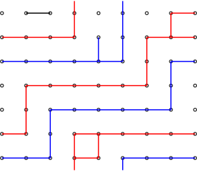
Figure 1: Cluster configuration with $j=2$ non-trivial clusters (NTC), here represented in red and blue colours. Each NTC is characterised by its number of branches, $n_{1}=2$, and by the permutation it realises, $P=(12)$. Within a given configuration, all NTC have the same topology.

Consider therefore first the case of a configuration having a single NTC. For the purpose of studying its topology, we can imagine that is has been shrunk to a line that winds the two periodic directions $(n_{1},n_{2})$ times. In our approach we focus on the the properties of the NTC along the direction of propagation of the transfer matrix ${\rm T}_{L}$, henceforth taken as the horizontal direction. If we imagine cutting the lattice along a vertical line, the NTC will be cut into $n_{1}$ horizontally percolating parts, which we shall call the $n_{1}$ branches of the NTC. Seen horizontally, a given NTC realises a permutation $P$ between the vertical coordinates of its $n_{1}$ branches, as shown in Fig. 1. Up to a trivial relabelling of the vertical coordinate, the permutation $P$ is independent of the horizontal coordinate of the (imaginary) vertical cut, and so, forms part of the topological description of the NTC. We thus describe totally the topology along the horizontal direction of a NTC by $n_{1}$ and the permutation $P\in S_{n_{1}}$.

Note that there are restrictions on the admissible permutations $P$. Firstly, $P$ cannot have any proper invariant subspace, or else the corresponding NTC would in fact correspond to several distinct NTC, each having a smaller value of $n_{1}$. For example, the case $n_{1}=4$ and $P=(13)(24)$ is not admissible, as $P$ corresponds in fact to two distinct NTC with $n_{1}=2$. In general, therefore, the admissible permutations $P$ for a given $n_{1}$ are simply cyclic permutations of $n_{1}$ coordinates. Secondly, planarity implies that the different branches of a NTC cannot intersect, and so not all cyclic permutations are admissible $P$. For example, the case $n_{1}=4$ and $P=(1324)$ is not admissible. In general the admissible cyclic permutations are characterised by having a constant coordinate difference between two consecutive branches, i.e., they are of the form $(k,2k,3k,\ldots)$ for some constant $k$, with all coordinates considered modulo $n_{1}$. For example, for $n_{1}=4$, the only admissible permutations are then finally $(1234)$ and $(1432)$.

Consider now the case of a configuration with several NTC. Recalling that all NTC belong to the same homotopy class, they must all be characterised by the same $n_{1}$ and $P$. Alternatively one can say that the branches of the different NTC are entangled. Henceforth we denote by $j$ the number of NTC with $n_{1}\geq 1$ in a given configuration. Note in particular that, seen along the horizontal direction, configurations with no NTC and configurations with one or more NTC percolating only vertically are topologically equivalent. This is an important limitation of our approach.

Let us denote by $Z_{j,n_{1},P}$ the partition function of the Potts model on an $L\times N$ torus, restricted to configurations with exactly $j$ NTC characterised by the index $n_{1}\geq 1$ and the permutation $P\in S_{n_{1}}$; if $P$ is not admissible, or if $n_{1}j>L$, we set $Z_{j,n_{1},P}=0$. Further, let $Z_{j,n_{1}}$ be the partition function restricted to configurations with $j$ NTC of index $n_{1}$, let $Z_{j}$ be the partition function restricted to configurations with $j$ NTC percolating horizontally, and let $Z$ be the total partition function. Obviously, we have $Z_{j,n_{1}}=\sum_{P\in S_{n_{1}}}Z_{j,n_{1},P}$, and $Z_{j}=\sum_{n_{1}=1}^{L}Z_{j,n_{1}}$, and $Z=\sum_{j=0}^{L}Z_{j}$. In particular, $Z_{0}$ corresponds to the partition function restricted to configurations with no NTC, or with NTC percolating only vertically.

In the case of a generic lattice all the $Z_{j,n_{1},P}$ are non-zero, provided that $P$ is an admissible cyclic permutation of length $n_{1}$, and that $n_{1}j\leq L$. The triangular lattice is a simple example of a generic lattice. Note however that other regular lattices may be unable to realise certain admissible $P$. For example, in the case of a square lattice or a honeycomb lattice, all $Z_{j,n_{1},P}$ with $n_{1}j=L$ and $n_{1}>1$ are zero, since there is not enough “space” on the lattice to permit all NTC branches to percolate horizontally while realising a non-trivial permutation. Such non-generic lattices introduce additional difficulties in the analysis which have to be considered on a case-to-case basis. In the following, we consider therefore the case of a generic lattice.

2.2 Structure of the transfer matrix

The construction and structure of the transfer matrix ${\rm T}$ can be taken over from the cyclic case [2]. In particular, we recall that ${\rm T}$ acts towards the right on states of connectivities between two time slices (left and right) and has a block-trigonal structure with respect to the number of bridges (connectivity components linking left and right) and a block-diagonal structure with respect to the residual connectivity among the non-bridged points on the left time slice. As before, we denote by ${\rm T}_{l}$ the diagonal block with a fixed number of bridges $l$ and a trivial residual connectivity. Each eigenvalue of ${\rm T}$ is also an eigenvalue of one or more ${\rm T}_{l}$. In analogy with [6] we shall sometimes call ${\rm T}_{l}$ the transfer matrix at level $l$. It acts on connectivity states which can be represented graphically as a partition of the $L$ points in the right time slice with a special marking (represented as a black point) of precisely $l$ distinct components of the partition (i.e., the components that are linked to the left time slice via a bridge).

A crucial difference with the cyclic case is that for a given partition of the right time slice, there are more possibilities for attributing the black points (for $0<l<L$). Considering for the moment the black points to be indistinguishable, we denote the corresponding dimension as $n_{\rm tor}(L,l)$. It can be shown [6] that

$$n_{\rm tor}(L,l)=\left\{\begin{array}[]{ll}\frac{1}{L+1}{2L\choose L}&\mbox{for }l=0\\ {2L-1\choose L-1}&\mbox{for }l=1\\ {2L\choose L-l}&\mbox{for }2\leq l\leq L\end{array}\right.$$ (2.1)

and clearly $n_{\rm tor}(L,l)=0$ for $l>L$.

Suppose now that a connectivity state at level $l$ is time evolved by a cluster configuration of index $n_{1}$ and corresponding to a permutation $P$. This can be represented graphically by adjoining the initial connectivity state to the left rim of the cluster configuration, as represented in Fig. 1, and reading off the final connectivity state as seen from the right rim of the cluster configuration. Evidently, the positions of the black points in the final state will be permuted with respect to their positions in the intial state, according to the permutation $P$. As we have seen, not all $P$ are admissible. We will show in the subsection 3.3 that the possible permutations at a given level $l$ (taking into account all the ways of attributing $l$ black points to cluster configurations) are the elements of the cyclic group $C_{l}$.the number of possible connectivity states without taking into account the possible permutations between black points, the dimension of $T_{l}$ is $l\;n_{\rm tor}(L,l)$, as $C_{l}$ has $l$ distinct elements.

Let us denote by $|v_{l,i}\rangle$ (where $1\leq i\leq n_{\rm tor}(L,l)$) the $n_{\rm tor}(L,l)$ standard connectivity states at level $l$. The full space of connectivities at level $l$, i.e., with $l$ distinguishable black points, can then be obtained by subjecting the $|v_{l,i}\rangle$ to permutations of the black points. It is obvious that ${\rm T}_{l}$ commutes with the permutations between black points (the physical reason being that ${\rm T}_{l}$ cannot “see” to which positions on the left time slice each bridge is attached). Therefore ${\rm T}_{l}$ itself has a block structure in a appropriate basis. Indeed, ${\rm T}_{l}$ can be decomposed into ${\rm T}_{l,D}$ where ${\rm T}_{l,D}$ is the restriction of ${\rm T}_{l}$ to the states transforming according to the irreducible representation (irrep) $D$ of $C_{l}$. Note that as $C_{l}$ is a abelian group of $l$ elements, it has $l$ irreps of dimension $1$. One can obtain the corresponding basis by applying the projectors $p_{D}$ on all the connectivity states at level $l$, where $p_{D}$ is given by

$$p_{D}=\frac{1}{l}\sum_{P}\bar{\chi}_{D}(P)\,P\;.$$ (2.2)

Here $\chi_{D}(P)$ is the character of $P$ in the irrep $D$ and $\bar{\chi}_{D}(P)$ is its complex conjugate. The application of all permutations of $C_{l}$ on any given standard vector $|v_{l,i}\rangle$ generates a regular representation of $C_{l}$, which contains therefore once each representation $D$ (of dimension $1$). As there are $n_{\rm tor}(L,l)$ standard vectors, the dimension of ${\rm T}_{l,D}$ is thus simply $n_{\rm tor}(L,l)$.

2.3 Definition of the $K_{l,D}$

We now define, as in the cyclic case [2], $K_{l}$ as the trace of $\left({\rm T}_{l}\right)^{N}$. Since ${\rm T}_{l}$ commutes with $C_{l}$, we can write

$$K_{l}=l\sum_{i=1}^{n_{\rm tor}(L,l)}\langle v_{l,i}|\left({\rm T}_{l}\right)^{N}|v_{l,i}\rangle\;.$$ (2.3)

In distinction with the cyclic case, we cannot decompose the partition function $Z$ over $K_{l}$ because of the possible permutations of black points (see below). We shall therefore resort to more elementary quantities, the $K_{l,D}$, which we define as the trace of $\left({\rm T}_{l,D}\right)^{N}$. Since both ${\rm T}_{l}$ and the projectors $p_{D}$ commute with $C_{l}$, we have

$$K_{l,D}=l\sum_{i=1}^{n_{\rm tor}(L,l)}\langle v_{l,i}|p_{D}\left({\rm T}_{l}\right)^{N}|v_{l,i}\rangle\;.$$ (2.4)

Obviously one has

$$K_{l}=\sum_{D}K_{l,D}\;,$$ (2.5)

the sum being over all the $l$ irreps $D$ of $C_{l}$. Recall that in the cyclic case the amplitudes of the eigenvalues at level $l$ are all identical. This is no longer the case, since the amplitudes depend on $D$ as well. Indeed

$$K_{l,D}=\sum_{k=1}^{n_{\rm tor}(L,l)}\left(\lambda_{l,D,k}\right)^{N}\;.$$ (2.6)

In order to decompose $Z$ over $K_{l,D}$ we will first use auxiliary quantities, the $K_{l,P_{l}}$ defined as:

$$K_{l,P_{l}}=\sum_{i=1}^{n_{\rm tor}(L,l)}\langle v_{l,i}|\left(P_{l}\right)^{-1}\left(T_{l}\right)^{N}|v_{l,i}\rangle\;,$$ (2.7)

$P_{l}$ being an element of the cyclic group $C_{l}$. So $K_{l,P_{l}}$ can be thought of as modified traces in which the final state differs from the initial state by the application of $P_{l}$. Note that $K_{l,{\rm Id}}$ is simply equal to $\frac{K_{l}}{l}$. Because of the possible permutations of the black points, the decomposition of $Z$ will contain not only the $K_{l,{\rm Id}}$ but also all the other $K_{l,P_{l}}$, with $P_{l}\in C_{l}$. We will show that the coefficients before $K_{l,P_{l}}$ coincide for all $P_{l}\in C_{l}$ that belong to the same class with respect to the symmetric group $S_{l}$. We will note these classes $(d_{i},n_{1})$ (corresponding to a level $l=d_{i}n_{1}$) and it is thus natural to define $K_{(d_{i},n_{1})}$ as:

$$K_{(d_{i},n_{1})}=\sum_{P_{l}\in(d_{i},n_{1})}K_{l,P_{l}}\;,$$ (2.8)

the sum being over elements $P_{l}\in C_{l}$ belonging to the class $(d_{i},n_{1})$. This definition will enable us to simplify some formulas, but ultimately we will come back to the $K_{l,P_{l}}$.

Once we will obtain the decomposition of $Z$ into $K_{l,P_{l}}$, we will need to express the $K_{l,P_{l}}$ in terms of the $K_{l,D}$ to obtain the decomposition of $Z$ into $K_{l,D}$, which are the quantities directly linked to the eigenvalues. Eqs. (2.4) and (2.2) yield a relation between $K_{l,D}$ and $K_{l,P_{l}}$:

$$K_{l,D}=\sum_{P_{l}}\chi_{D}(P_{l})K_{l,P_{l}}\;.$$ (2.9)

These relations can be inverted so as to obtain $K_{l,P_{l}}$ in terms of $K_{l,D}$, since the number of elements of $C_{l}$ equals the number of irreps $D$ of $C_{l}$. Multiplying Eq. (2.9) by $\bar{\chi}_{D}(P^{\prime}_{l})$ and summing over $D$, and using the orthogonality relation $\sum_{D}\bar{\chi}_{D}(P_{l})\chi_{D}(P^{\prime}_{l})=l\delta_{P_{l},P^{\prime}_{l}}$ one easily deduces that:

$$K_{l,P_{l}}=\sum_{D}\frac{\bar{\chi}_{D}(P_{l})}{l}K_{l,D}$$ (2.10)

Note that

$$\sum_{D}\bar{\chi}_{D}(P_{l})=l\,\delta_{P_{l},{\rm Id}}$$ (2.11)

2.4 Useful properties of the group $C_{l}$

In the following we will obtain an expression of the amplitudes at the level $l$ which involves sums of characters of the irreps $D$ of $C_{l}$. In order to reobtain Eq. (1.2), we will have to calculate these sums. We give here the results we shall need.

$C_{l}$ is the group generated by the permutation $E_{l}=(12\dots l)$. It is abelian and consists of the $l$ elements $E_{l}^{a}=(E_{l})^{a}$, with $1\leq a\leq l$. The cycle structure of these elements is given by a simple rule. We denote by $d_{i}$ (with $1\leq i\leq q(l)$) the integer divisors of $l$ (in particular $d_{1}=1$ and $d_{q(l)}=l$), and by $A_{d_{i}}$ the set of integers which are a product of $d_{i}$ by an integer $n$ such that $1\leq n\leq\frac{l}{d_{i}}$ and $n\wedge\frac{l}{d_{i}}=1$, If $a\in A_{d_{i}}$ then $E_{l}^{a}$ consists of $d_{i}$ entangled cycles of the same length $\frac{l}{d_{i}}$. We denote the corresponding class $\left(d_{i},\frac{l}{d_{i}}\right)$. The number of elements of $A_{l_{i}}$, and so the number of such $E_{l}^{a}$, is equal to $\phi\left(\frac{l}{d_{i}}\right)$, where $\phi$ is Euler’s totient function whose definition has been recalled in the introduction.

Consider $C_{6}$ as an example. The elements of $C_{6}$ in the class $(1,6)$ are $E_{6}=(123456)$ and $E_{6}^{5}=(165432)$. The elements in $(2,3)$ are $E_{6}^{2}=(135)(246)$ and $E_{6}^{4}=(153)(264)$. There is only one element $E_{6}^{3}=(14)(25)(36)$ in $(3,2)$, and only $E_{6}^{6}={\rm Id}$ in $(6,1)$. Indeed, the integer divisors of $6$ are $1$, $2$, $3$, $6$, and we have $A_{1}=\{1,5\}$, $A_{2}=\{2,4\}$, $A_{3}=\{3\}$, $A_{6}=\{6\}$.

$C_{l}$ has $l$ irreps denoted $D_{k}$, with $1\leq k\leq l$. The corresponding characters are given by $\chi_{D_{k}}\left(E_{l}^{a}\right)=\exp\left(-i2\pi\frac{ka}{l}\right)$. We will have to calculate in the following the sums given by:

$$\sum_{P_{l}\in\left(d_{i},\frac{l}{d_{i}}\right)}\bar{\chi}_{D_{k}}(P_{l})=\sum_{a\in A_{d_{i}}}\exp\left(i2\pi\frac{ka}{l}\right)\;.$$ (2.12)

These sums are slight generalizations of Ramanujan’s sums. Using Theorem $272$ of Ref. [5], we obtain that:

$$\sum_{P_{l}\in\left(d_{i},\frac{l}{d_{i}}\right)}\bar{\chi}_{D_{k}}(P_{l})=\frac{\mu\left(\frac{m}{m\wedge d_{i}}\right)\phi\left(\frac{l}{d_{i}}\right)}{\phi\left(\frac{m}{m\wedge d_{i}}\right)}\;,$$ (2.13)

where $k$ is supposed to be in $A_{d}$ and $m$ is given by $\frac{l}{d}$. The Möbius function $\mu$ has been defined in the Introduction. Note that all $k$ which are in the same $A_{d}$ lead to the same sum; we can therefore restrain ourselves to $k$ equal to an integer divisor of $l$ in order to have the different values of these sums. Indeed, we will label the different amplitudes at level $l$ by $m$.

3 Decomposition of the partition function

3.1 The characters $K_{l}$

By generalising the working for the cyclic case, we can now obtain a decomposition of the $K_{l}$ in terms of the $Z_{j,n_{1}}$. To that end, we first determine the number of states $|v_{l,i}\rangle$ which are compatible with a given configuration of $Z_{j,n_{1}}$, i.e., the number of initial states $|v_{l,i}\rangle$ which are thus that the action by the given configuration produces an identical final state. The notion of compatibility is illustrated in Fig. 2.

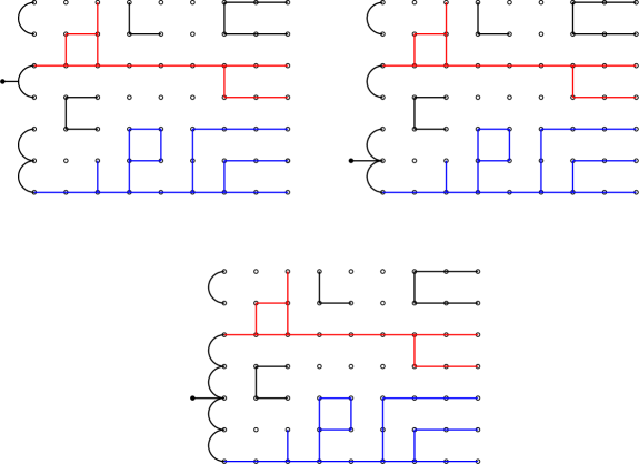
Figure 2: Standard connectivity states at level $l=1$ which are compatible with a given cluster configuration contributing to $Z_{2,1}$.

We consider first the case $n_{1}=1$ and suppose that the $k$’th NTC connects onto the points $\{y_{k}\}$. The rules for constructing the compatible $|v_{l,i}\rangle$ are identical to those of the cyclic case:

1. The points $y\notin\cup_{k=1}^{j}\{y_{k}\}$ must be connected in the same way in $|v_{l,i}\rangle$ as in the cluster configuration.

2. The points $\{y_{k}\}$ within the same bridge must be connected in $|v_{l,i}\rangle$.

3. One can independently choose to associate or not a black point to each of the sets $\{y_{k}\}$. One is free to connect or not two distinct sets $\{y_{k}\}$ and $\{y_{k^{\prime}}\}$.

The choices mentioned in rule 3 leave $n_{\rm tor}(j,l)$ possibilities for constructing a compatible $|v_{l,i}\rangle$. The coefficient of $Z_{j,1}$ in the decomposition of $K_{l}$ is therefore $\frac{l\;n_{\rm tor}(j,l)}{Q^{j}}$, since the allowed permutation of black points in a standard vector $|v_{l,i}\rangle$ allows for the construction of $l$ distinct states, and since the weight of the $j$ NTC in $K_{l}$ is $1$ instead of $Q^{j}$. It follows that

$$K_{l}=\sum_{j=l}^{L}l\,n_{\rm tor}(j,l)\frac{Z_{j,1}}{Q^{j}}\qquad\mbox{for }n_{1}=1.$$ (3.1)

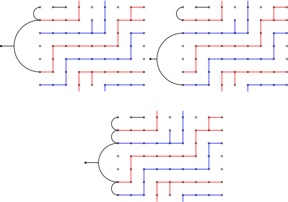
Figure 3: Standard connectivity states at level $l=1$ which are compatible with a given cluster configuration contributing to $Z_{2,2}$.

We next consider the case $n_{1}>1$. Let us denote by $\{y_{k,m}\}$ the points that connect onto the $m$’th branch of the $k$’th NTC (with $1\leq m\leq n_{1}$ and $1\leq k\leq j$), and by $\{y_{k}\}=\cup_{m=1}^{n_{1}}\{y_{k,m}\}$ all the points that connect onto the $k$’th NTC. As shown in Fig. 3, the $|v_{l,i}\rangle$ which are compatible with this configuration are such that

1. The connectivities of the points $y\notin\cup_{k=1}^{j}\{y_{k}\}$ are identical to those appearing in the cluster configuration.

2. All points $\{y_{k,m}\}$ corresponding to the branch of a NTC must be connected.

3. We must now count the number of ways we can link the branches of the $k$ NTC and attribute $l$ black points so that the connection and the position of the black points are unchanged after action of the cluster configuration. For $l\geq 2$, there are no compatible states (indeed it is not possible to respect planarity and to leave the position of the black points unchanged). For $l=1$ and $l=0$ there are respectively ${2j-1\choose j}=\frac{1}{2}\cdot{2j\choose j}$ and ${2j\choose j}$ compatible states. Note that these results do not depend on the precise value of $n_{1}$ (for $n_{1}>1$).

The rule $3$ implies that the decomposition of $K_{l}$ with $l\geq 2$ does not contain any of the $Z_{j,n_{1}}$ with $n_{1}>1$. We therefore have simply

$$K_{l}=\sum_{j=l}^{L}l\,n_{\rm tor}(j,l)\frac{Z_{j,1}}{Q^{j}}\qquad\mbox{for }l\geq 2\;.$$ (3.2)

The decomposition of $K_{1}$ and $K_{0}$ are given by:

$$K_{1}=\sum_{j=1}^{L}n_{\rm tor}(j,1)\frac{Z_{j,1}}{Q^{j}}+\sum_{j=1}^{\left\lfloor\frac{L}{2}\right\rfloor}\frac{{2j\choose j}}{2}\frac{Z_{j,n_{1}>1}}{Q^{j}}$$ (3.3)

$$K_{0}=\sum_{j=0}^{L}n_{\rm tor}(j,0)\frac{Z_{j,1}}{Q^{j}}+\sum_{j=1}^{\left\lfloor\frac{L}{2}\right\rfloor}{2j\choose j}\,\frac{Z_{j,n_{1}>1}}{Q^{j}}\;.$$ (3.4)

Note that the coefficients in front of $Z_{j,n_{1}}$ do not depend on the precise value of $n_{1}$ when $n_{1}>1$. To simplify the notation we have defined $Z_{0,1}=Z_{0}$.

3.2 The coefficients $b^{(l)}$

Since the coefficients in front of $Z_{j,1}$ and $Z_{j,n_{1}>1}$ in Eqs. (3.3)–(3.4) are different, we cannot invert the system of relations (3.2)–(3.4) so as to obtain $Z_{j}\equiv Z_{j,1}+Z_{j,n_{1}>1}$ in terms of the $K_{l}$. It is thus precisely because of NTC with several branches contributing to $Z_{j,n_{1}>1}$ that the problem is more complicated than in the cyclic case.

In order to appreciate this effect, and compare with the precise results that we shall find later, let us for a moment assume that Eq. (3.2) were valid also for $l=0,1$. We would then obtain

$$Z_{j,1}=\sum_{l=j}^{L}b_{j}^{(l)}\frac{K_{l}}{l}\;,$$ (3.5)

where the coefficients $b^{(l)}_{j}$ have already been defined in Eq. (1.5). The coefficients $b^{(l)}$ play a role analogous to those denoted $c^{(l)}$ in the cyclic case [2]; note also that $b^{(l)}=c^{(l)}$ for $l\leq 2$. Chang and Schrock have developed a diagrammatic technique for obtaining the $b^{(l)}$ [6].

Supposing still the unconditional validity of Eq. (3.2), one would obtain for the full partition function

$$Z=\sum_{l=0}^{L}b^{(l)}\frac{K_{l}}{l}\;.$$ (3.6)

This relation will be modified due to the terms $Z_{j,n_{1}>1}$ realising permutations of the black points, which we have here disregarded. To get things right we shall introduce irrep dependent coefficients $b^{(l,D)}$ and write $Z=\sum_{l=0}^{L}\sum_{D}b^{(l,D)}K_{l,D}$. Neglecting $Z_{j,n_{1}>1}$ terms would lead, according to Eq. (3.6), to $b^{(l,D)}=\frac{b^{(l)}}{l}$ independently of $D$. We shall see that the $Z_{j,n_{1}>1}$ will lift this degeneracy of amplitudes in a particular way, since there exist certain relations between the $b^{(l,D)}$ and the $b^{(l)}$.

In order to simplify the formulas we will obtain later, we define the coefficients $\tilde{b}^{(l)}$ for $l\geq 1$ by:

$$\tilde{b}^{(l)}=\sum_{j=0}^{l}(-1)^{l-j}\frac{2l}{l+j}{l+j\choose l-j}Q^{j}+(-1)^{l}(Q-1)\;.$$ (3.7)

For $l\geq 2$, $\tilde{b}^{(l)}$ is simply equal to $b^{(l)}$, they are different only for $l=1$, as we have $b^{(1)}=Q-1$ but $\tilde{b}^{(1)}=-1$. In order to reobtain the expression (1.2) of Read and Saleur for the amplitudes we will use that:

$$\tilde{b}^{(l)}=2\cos(2\pi le_{0})+(-1)^{l}(Q-1)\;,$$ (3.8)

where $e_{0}$ has been defined in Eq. (1.4).

3.3 Decomposition of the $K_{l,P_{l}}$

The relations (3.2)–(3.4) were not invertible due to an insufficient number of elementary quantities $K_{l}$. Let us now show how to produce a development in terms of $K_{l,P_{l}}$, i.e., taking into account the possible permutations of black points. This development turns out to be invertible.

A standard connectivity state with $l$ black points is said to be $P_{l}$-compatible with a given cluster configuration if the action of that cluster configuration on the connectivity state produces a final state that differs from the initial one just by a permutation $P_{l}$ of the black points. This generalises the notion of compatibility used in Sec. 3.1 to take into account the permutations of black points.

Let us first count the number of standard connectivities $|v_{l,i}\rangle$ which are $P_{l}$-compatible with a cluster configuration contributing to $Z_{j,n_{1},P}$. For $n_{1}=1$, $S_{n_{1}}$ contains only the identity element ${\rm Id}$, and so the results of Sec. 3.1 apply: the $Z_{j,1}$ contribute only to $K_{l,{\rm Id}}$. We consider next a configuration contributing to $Z_{j,n_{1},P}$ with $n_{1}>1$. The $|v_{l,i}\rangle$ which are $P_{l}$-compatible with this configuration satisfy the same three rules as given in Sec. 3.1 for the case $n_{1}>1$, with the slight modification of rule 3 that the black points must be attributed in such a way that the final state differs from the initial one by a permutation $P_{l}$.

This modification makes the attribution of black points considerably more involved than was the case in Sec. 3.1. First note that not all the $P_{l}$ are admissible. To be precise, the cycle decomposition of the allowed permutations can only contain $P$, as $P$ is the permutation between the branches realised by a single NTC. Therefore the admissible permutations contain only $P$ and are such that $l=d_{i}n_{1}$, denoting by $d_{i}$ the number of times $P$ is contained. We note $(d_{i},n_{1})$ the corresponding classes of permutations and $K_{(d_{i},n_{1})}$ the corresponding $K$, see Eq. (2.8). Note that the number of classes of admissible permutations at a given level $l$ is equal to the number of integers $d_{i}$ dividing $l$, i.e. $q(l)$. Furthermore, inside these classes, not all permutations are admissible. Indeed, the entanglement of the NTC imply the entanglement of the structure of the allowed permutations. We deduce from all this rules that, as announced, the admissible permutations at level $l$ are simply the elements of the cyclic group $C_{l}$.

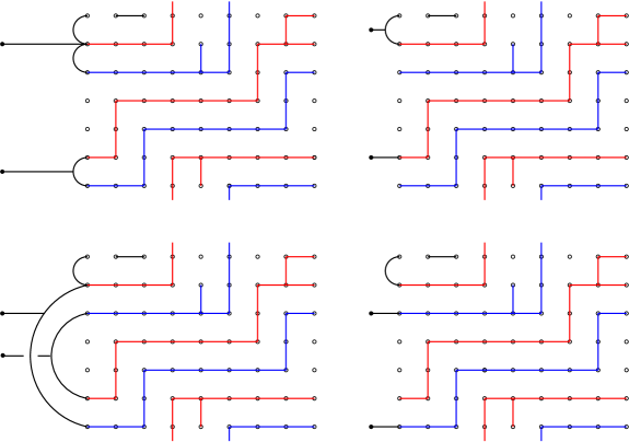
Figure 4: Standard connectivity states at level $l=2$ which are $(12)$-compatible with a given cluster configuration contributing to $Z_{2,2}$. The action of the cluster configuration on these connectivity states permutes the positions of the two black points.

Let us now consider the decomposition of $K_{l,P_{l}}$, which is depicted in Fig. 4, $P_{l}$ being an authorized permutation different from identity and containing $d_{i}$ times the permutation $P$ of length $n_{1}$. Then, only the $Z_{j,n_{1},P}$, with $j\geq d_{i}$, contribute to the decomposition of $K_{l,P_{l}}$. We find that the number of $|v_{l,i}\rangle$ which are $P_{l}$-compatible with a given clusters configuration of $Z_{j,n_{1},P}$ is ${2j\choose j-d_{i}}$. Therefore we have:

$$K_{l,P_{l}}=\sum_{j=d_{i}}^{\left\lfloor\frac{L}{n_{1}}\right\rfloor}{2j\choose j-d_{i}}\frac{Z_{j,n_{1},P}}{Q^{j}}\;.$$ (3.9)

From this we infer the decomposition of $K_{(d_{i},n_{1})}$:

$$K_{(d_{i},n_{1})}=\sum_{j=d_{i}}^{\left\lfloor\frac{L}{n_{1}}\right\rfloor}{2j\choose j-d_{i}}\frac{Z_{j,n_{1}}}{Q^{j}}\;.$$ (3.10)

We will use the decomposition of $K_{(d_{i},n_{1})}$ in the following as it is simplier to work with $Z_{j,n_{1}}$ than with $Z_{j,n_{1},P}$ (but one could consider the $Z_{j,n_{1},P}$ too).

It remains to study the special case of $P_{l}={\rm Id}$. This is in fact trivial. Indeed, in that case, the value of $n_{1}$ in $Z_{j,n_{1}}$ is no longer fixed, and one must sum over all possible values of $n_{1}$, taking into account that the case of $n_{1}=1$ is particular. Since $K_{l,{\rm Id}}=\frac{K_{l}}{l}$, one obtains simply Eqs. (3.2)–(3.4) of Sec. 3.1 up to a global factor.

3.4 Decomposition of $Z_{j}$ over the $K_{l,P_{l}}$

To obtain the decomposition of $Z_{j,n_{1}}$ in terms of the $K_{l,P_{l}}$, we invert Eq. (3.10) for varying $d_{i}$ and fixed $n_{1}>1$ and we obtain:

$$Z_{j,n_{1}}=Q^{j}\sum_{d_{i}=j}^{\left\lfloor\frac{L}{n_{1}}\right\rfloor}(-1)^{d_{i}-j}\frac{2d_{i}}{d_{i}+j}{d_{i}+j\choose d_{i}-j}K_{(d_{i},n_{1})}\qquad\mbox{for }n_{1}>1\;.$$ (3.11)

Since the coefficients in this sum do not depend on $n_{1}$ (provided that $n_{1}>1$), we can sum this relation over $n_{1}$ and write it as

$$Z_{j,n_{1}>1}=Q^{j}\sum_{d_{i}=j}^{\left\lfloor\frac{L}{2}\right\rfloor}(-1)^{d_{i}-j}\frac{2d_{i}}{d_{i}+j}{d_{i}+j\choose d_{i}-j}K_{(d_{i},n_{1}>1)}$$ (3.12)

where we recall the notations $Z_{j,n_{1}>1}=\sum_{n_{1}=2}^{L}Z_{j,n_{1}}$ and $K_{(d_{i},n_{1}>1)}=\sum_{n_{1}=2}^{L}K_{(d_{i},n_{1})}$, corresponding to permutations consisting of $d_{i}$ cycles of the same length $>1$.

Consider next the case $n_{1}=1$. For $j\geq 2$ one has simply

$$Z_{j,1}=\sum_{l=j}^{L}\frac{b^{(l)}_{j}}{l}K_{l}\;,$$ (3.13)

recalling Eq. (3.5) and the fact that for $l\geq 2$ the $Z_{j,n_{1}>1}$ do not appear in the decomposition of $K_{l}$. However, according to Eqs. (3.3)–(3.4), the $Z_{j,n_{1}>1}$ do appear for $l=0$ and $l=1$, and one obtains

$$Z_{1,1}=\sum_{l=1}^{L}\frac{b^{(l)}_{1}}{l}K_{l}-\frac{Q}{2}\sum_{j=1}^{\left\lfloor\frac{L}{2}\right\rfloor}{2j\choose j}\frac{Z_{j,n_{1}>1}}{Q^{j}}\;.$$ (3.14)

Inserting the decomposition (3.12) of $Z_{j,n_{1}>1}$ into Eq. (3.14) one obtains the decomposition of $Z_{1,1}$ over $K_{l}$ and $K_{(d_{i},n_{1})}$:

$$Z_{1,1}=\sum_{l=1}^{L}\frac{b^{(l)}_{1}}{l}K_{l}+Q\sum_{d_{i}=1}^{\left\lfloor\frac{L}{2}\right\rfloor}(-1)^{d_{i}}K_{(d_{i},n_{1}>1)}\;.$$ (3.15)

We proceed in the same fashion for the decomposition of $Z_{0}\equiv Z_{0,1}$, finding

$$Z_{0}=\sum_{l=0}^{L}\frac{b^{(l)}_{0}}{l}K_{l}-\frac{1}{2}\sum_{j=1}^{\left\lfloor\frac{L}{2}\right\rfloor}{2j\choose j}\frac{Z_{j,n_{1}>1}}{Q^{j}}\;.$$ (3.16)

Upon insertion of the decomposition (3.12) of $Z_{j,n_{1}>1}$, one arrives at

$$Z_{0}=\sum_{l=0}^{L}\frac{b^{(l)}_{0}}{l}K_{l}+\sum_{d_{i}=1}^{\left\lfloor\frac{L}{2}\right\rfloor}(-1)^{d_{i}}K_{(d_{i},n_{1}>1)}\;.$$ (3.17)

Since $Z_{j}=Z_{j,1}+Z_{j,n_{1}>1}$, we conclude from Eqs. (3.13)–(3.12) and from Eq. (3.7) that, for any $j$,

$$Z_{j}=\sum_{l=j}^{L}\frac{b^{(l)}_{j}}{l}K_{l}+\sum_{d_{i}=j}^{\left\lfloor\frac{L}{2}\right\rfloor}\tilde{b}^{(d_{i})}_{j}K_{(d_{i},n_{1}>1)}\;.$$ (3.18)

The decomposition of $Z\equiv\sum_{0\leq j\leq L}Z_{j}$ is therefore

$$Z=\sum_{l=0}^{L}\frac{b^{(l)}}{l}K_{l}+\sum_{d_{i}=1}^{\left\lfloor\frac{L}{2}\right\rfloor}\tilde{b}^{(d_{i})}K_{(d_{i},n_{1}>1)}\;.$$ (3.19)

4 Amplitudes of the eigenvalues

4.1 Decomposition of $Z$ over the $K_{l,D}$

The culmination of the preceeding section was the decomposition (3.18) of $Z_{j}$ in terms of $K_{l,P_{l}}$ (as $K_{(d_{i},n_{1})}$ is the sum of the $K_{l,P_{l}}$ with $P_{l}$ being an element of $C_{l}$ belonging to the class $(d_{i},n_{1})$). However, it is the $K_{l,D}$ which are directly related to the eigenvalues of the transfer matrix ${\rm T}$. For that reason, we now use the relation (2.10) between the $K_{l,P_{l}}$ and the $K_{l,D_{k}}$ to obtain the decomposition of $Z_{j}$ in terms of $K_{l,D_{k}}$. The result is:

$$Z_{j}=\sum_{l,D_{k}}b^{(l,D_{k})}_{j}K_{l,D_{k}}$$ (4.1)

where the coefficients $b^{(l,D_{k})}_{j}$ are given by

$$b^{(l,D_{k})}_{j}=\frac{b^{(l)}_{j}}{l}+\sum_{(d_{i}<l)|l}\frac{\tilde{b}^{(d_{i})}_{j}}{l}\;\sum_{P_{l}\in\left(d_{i},\frac{l}{d_{i}}\right)}\bar{\chi}_{D_{k}}(P_{l})\;.$$ (4.2)

Indeed, $K_{l}=\sum_{D_{k}}K_{l,D_{k}}$, and since $K_{(d_{i},n_{1})}$ corresponds to the level $l=d_{i}n_{1}$, we have $K_{(d_{i},n_{1})}=\sum_{D_{k}\in C_{d_{i}n_{1}}}\frac{\bar{\chi}_{D_{k}}((d_{i},n_{1}))}{l}K_{d_{i}n_{1},D_{k}}$. (Recall that $(d_{i},n_{1})$ is the class of permutations consisting of $d_{i}$ cycles of the same length $n_{1}=\frac{l}{d_{i}}$.) As explained in Sec. 3.2, the $b^{(l,D_{k})}_{j}$ are not simply equal to $\frac{b^{(l)}_{j}}{l}$ because of the $n_{1}>1$ terms. Using Eq. (2.11) we find that they nevertheless obey the following relation

$$\sum_{D_{k}\in C_{l}}b^{(l,D_{k})}_{j}=b^{(l)}_{j}\;.$$ (4.3)

But from Eq. (4.2) the $b^{(l,D_{k})}_{j}$ with $l<2j$ are trivial, i.e., equal to $\frac{b^{(l)}_{j}}{l}$ independently of $D$. This could have been shown directly by considering the decomposition (3.2) of $K_{l}$.

The decomposition of $Z$ over $K_{l,D_{k}}$ is obviously given by

$$Z=\sum_{l,D_{k}}b^{(l,D_{k})}K_{l,D_{k}}$$ (4.4)

where

$$b^{(l,D_{k})}=\sum_{j=1}^{l}b^{(l,D_{k})}_{j}\;,$$ (4.5)

i.e.

$$b^{(l,D_{k})}=\frac{b^{(l)}}{l}+\sum_{(d_{i}<l)|l}\frac{\tilde{b}^{(d_{i})}}{l}\;\sum_{P_{l}\in\left(d_{i},\frac{l}{d_{i}}\right)}\bar{\chi}_{D_{k}}(P_{l})\;.$$ (4.6)

This is the central result of our article: we have obtained a rather simple expression of the amplitudes $b^{(l,D)}$ in terms of the characters of the irrep $D$. A priori, for a given level $l$, there should be $l$ distinct amplitudes $b^{(l,D)}$ because $C_{l}$ has $l$ distinct irreps $D$. However, because of the fact that two different permutations in the same class $\left(d_{i},\frac{l}{d_{i}}\right)$ correspond to the same coefficient $b^{(d_{i})}$, there are less distinct amplitudes: some $b^{(l,D)}$ are the same. Indeed, the Eq. (4.6) giving the amplitudes of the eigenvalues contains generalized Ramanujan’s sum, so using the subsection 2.4, the $D_{k}$ whose $k$ are in the same $A_{d}$ correspond to the same amplitude $b^{(l,D_{d})}$. For example, at level $6$, there are only four distinct amplitudes: $b^{(6,D_{1})}$, $b^{(6,D_{2})}$, $b^{(6,D_{3})}$ and $b^{(6,D_{6})}$, since we have $b^{(6,D_{1})}=b^{(6,D_{5})}$ and $b^{(6,D_{2})}=b^{(6,D_{4})}$.

An important consequence of the expression of the $b^{(l,D_{k})}$ is that they satisfy

$$\sum_{D_{k}\in C_{l}}b^{(l,D_{k})}=b^{(l)}\;,$$ (4.7)

i.e., the sum of the $l$ (not necessarily distinct) amplitudes $b^{(l,D_{k})}$ at level $l$ is equal to $b^{(l)}$. This has been previously noted by Chang and Shrock [6], except that they stated it was the sum of $l!$ amplitudes, not $l$, as they did not notice that only permutations in the cyclic group $C_{l}$ were admissible.

Note also that for $l\geq 2$, Eq. (4.6) can be written more simply as:

$$b^{(l,D_{k})}=\sum_{d_{i}|l}\frac{\tilde{b}^{(d_{i})}}{l}\;\sum_{P_{l}\in\left(d_{i},\frac{l}{d_{i}}\right)}\bar{\chi}_{D_{k}}(P_{l})\;,$$ (4.8)

since $b^{(l)}=\tilde{b}^{(l)}$ for $l\geq 2$. We now restrict ourselves to this case, as the amplitudes at levels $0$ and $1$ are simply $b^{(0)}=1$ and $b^{(1)}=Q-1$.

4.2 Compact formula for the amplitudes

We now calculate the Ramanujan’s sums appearing in Eq. (4.8). Using Eq. (2.13), we obtain:

$$b^{(l,m)}=\sum_{d_{i}|l}\frac{\mu\left(\frac{m}{m\wedge d_{i}}\right)\phi\left(\frac{l}{d_{i}}\right)}{l\phi\left(\frac{m}{m\wedge d_{i}}\right)}\;\tilde{b}^{(d_{i})}$$ (4.9)

Remember that $m$ is given by $\frac{l}{d}$ for $k$ in the set $A_{d}$, and so is an integer divisor of $l$. Using the expression of the $\tilde{b}^{(d_{i})}$ given in Eq. (3.8), we finally recover the formula (1.2) of Read and Saleur. In particular, the term $(-1)^{l}(Q-1)$ in the definition (3.7) of $\tilde{b}^{(l)}$ corresponds to degenerate cluster configurations.

Note that the number of different amplitudes at level $l$ is simply equal to the number of integer divisors of $l$. In particular, when $l$ is prime, there are only two different amplitudes: $b^{(l,1)}$ which corresponds to $b^{(l,D_{l})}$ ($D_{l}$ is the identity representation) and $b^{(l,l)}$ which corresponds to the $l-1$ other $b^{(l,D_{k})}$ (as they are all equal). Using that $b^{(1)}=-1$, we find:

$$b^{(l,1)} = \frac{b^{(l)}-l+1}{l}$$ (4.10)

$$b^{(l,l)} = \frac{b^{(l)}+1}{l}$$ (4.11)

This could have been simply directly showed using Eq. (4.8). Indeed, for $l$ prime, $C_{l}$ contains ${\rm Id}$ and $l-1$ cycles of length $l$. As $b^{(1)}=-1$, we deduce that $b^{(l,1)}=\frac{b^{(l)}-l+1}{l}$. For $b^{(l,l)}$, one needs just use that $\sum_{k=1}^{l-1}\exp\left(\frac{i2\pi k}{l}\right)=-1$.

5 Conclusion

To summarise, we have generalised the combinatorial approach developed in Ref. [2] for cyclic boundary conditions to the case of toroidal boundary conditions. In particular, we have obtained the decomposition of the partition function for the Potts model on finite tori in terms of the generalised characters $K_{l,D}$. We proved that the formula (1.2) of Read and Saleur is valid for any finite lattice, and for any inhomogeneous choice of the coupling constants. Furthermore, our physical interpretation of this formula is new and is based on the cyclic group $C_{l}$.

The eigenvalue amplitudes are instrumental in determining the physics of the Potts model, in particular in the antiferromagnetic regime [11, 12]. Generically, this regime belongs to a so-called Berker-Kadanoff (BK) phase in which the temperature variable is irrelevant in the renormalisation group sense, and whose properties can be obtained by analytic continuation of the well-known ferromagnetic phase transition [11]. Due to the Beraha-Kahane-Weiss (BKW) theorem [13], partition function zeros accumulate at the values of $Q$ where either the amplitude of the dominant eigenvalue vanishes, or where the two dominant eigenvalues become equimodular. When this happens, the BK phase disappears, and the system undergoes a phase transition with control parameter $Q$. Determining analytically the eigenvalue amplitudes is thus directly relevant for the first of the hypotheses in the BKW theorem.

For the cyclic geometry, the amplitudes are very simple, and the real values of $Q$ satisfying the hypothesis of the BKW theorem are simply the so-called Beraha numbers, $Q=B_{n}=(2\cos(\pi/n))^{2}$ with $n=2,3,\ldots$, independently of the width $L$. For the toroidal case, the formula is more complicated, and there can be degeneracies of eigenvalues between different levels which depend on the width $L$ of the lattice, as shown by Chang and Shrock [6]. The role of the Beraha numbers will therefore be considered in a future work.

Acknowledgments.

The authors are grateful to H. Saleur, J.-B. Zuber and P. Zinn-Justin for some useful discussions. We also thank J. Salas for collaboration on closely related projects.

References

- [1] P.W. Kasteleyn and C.M. Fortuin, J. Phys. Soc. Jap. Suppl. 26, 11 (1969); C.M. Fortuin and P.W. Kasteleyn, Physica 57, 536 (1972).
- [2] J.-F. Richard and J.L. Jacobsen, Nucl. Phys. B 750, 250–264 (2006); math-ph/0605016.
- [3] N. Read and H. Saleur, Nucl. Phys. B 613, 409 (2001); hep-th/0106124.
- [4] P. Di Francesco, H. Saleur and J.B. Zuber, J. Stat. Phys. 49, 57 (1987).
- [5] G. H. Hardy and E. M. Wright An Introduction to the Theory of Numbers (Oxford Science Publications, New York, 1979).
- [6] S.-C. Chang and R. Shrock, Physica A 364, 231–262 (2006); cond-mat/0506274.
- [7] A. Nichols, J. Stat. Mech. 0601, 3 (2006); hep-th/0509069.
- [8] J.-F. Richard and J.L. Jacobsen, Nucl. Phys. B 750, 229–249 (2006); math-ph/0605015.
- [9] V. Pasquier, J. Phys. A 20, L1229 (1987).
- [10] J.-F. Richard and J.L. Jacobsen, Nucl. Phys. B 731, 335 (2005); math-ph/0507048.
- [11] H. Saleur, Commun. Math. Phys. 132, 657 (1990); Nucl. Phys. B 360, 219 (1991).
- [12] J.L. Jacobsen and H. Saleur, Nucl. Phys. B 743, 207 (2006); cond-mat/0512056.
- [13] S. Beraha, J. Kahane and N.J. Weiss, Proc. Natl. Acad. Sci. USA 72, 4209 (1975).