Numerical Calculation of a Minimal Surface Using Bilinear Interpolations and
Chebyshev Polynomials.

Abstract

We calculate the minimal surface bounded by four-sided figures whose projection on a plane is a rectangle, starting with the bilinear interpolation and using, for smoothness, the Chebyshev polynomial expansion in our discretized numerical algorithm to get closer to satisfying the zero mean curvature condition. We report values for both the bilinear and improved areas, suggesting a quantitative evaluation of the bilinear interpolation. An analytical expression of the Schwarz minimal surface with polygonal boundaries and its 3-dimensional plot is also given.

1 Introduction

In mathematical modeling it is not uncommon to need a surface that spans a known boundary and has the least value of a related quantity, say, area. If the least area is desired, the problem is termed in the mathematical literature as the Plateau problem, namely minimizing the area functional

$$A(X)=\int\int_{\Omega}|X_{u}\times X_{v}|\,du\,dv.$$ (1)

Here $\Omega\subset R^{2}$ is a domain over which the surface $X$ is defined as a map, with the boundary condition $X(\partial\Omega)=\Gamma$. It is known [1] that the first variation of $A(X)$ vanishes if and only if the mean curvature $H$ of $X$ is zero everywhere in it. Thus to get a minimal (or, more precisely, a stationary) surface, we have to solve the differential equation obtained by setting the mean curvature $H$ equal to zero for each value of the two parameters, say, $u$ and $v$ parameterizing a surface spanning the fixed boundary. In a numerical work, the problem has to be discretized by choosing a selection of the numerical values of the two parameters and finding the minimal- surface-position for each pair of the values. If the given boundary is a four-sided figure whose projection on a plane is a rectangle, the surface positions become simply the heights above the $uv$-plane. Such ‘numerical heights’ and resulting ‘numerical minimal surfaces’ have been computed in ref. [8] for a variety of closed curve boundaries.

In this paper, we report, in the section 4 below, a modification to their algorithm that uses linear combinations of the Chebyshev polynomials as heights at the discretized $uv$-positions. In this way, we replace in the algorithm arbitrary heights by linear combinations of convenient polynomials with arbitrary coefficients.

The immediate advantage of this use of polynomials has been a reduction in the discretization error and a better convergence. Polynomials are (smooth) analytic functions having simply calculable derivatives. We have also carried further our efforts to find analytic surfaces that can be taken as ‘approximate minimal surfaces’:

1) We read initial heights from a ruled analytic surface spanning our fixed boundary, namely the bilinear interpolation introduced in the section 3. And for knowing how much heights changed through our numerical minimization

2) we compared the areas of the numerically found points (or ‘numerical minimal surface’ explained in section 4.2 with those of the bilinear interpolation for each of the selected boundaries.

Through this quantitative comparison, something missing in the previous works, we suggest to a user of a minimal surface bounded by four straight lines a prescription that may well save almost all the computer programming and CPU time spent in implementation, say, the algorithm of refs. [8]: the approximate equality of the areas of the bilinear interpolation and numerical minimal surface strongly suggests that the simple bilinear interpolation itself may work as a ‘minimal surface’ for many mathematical models that need minimal surfaces bounded by four straight lines.

The only ruled surface, other than the plane, which is a minimal surface is a helicoid [1]. As one boundary of a helicoid must be part of a helix, which is not a straight line, the boundary of a helicoid cannot be composed of four straight lines. In this way there cannot be at least a ruled surface which is a minimal surface bounded by four straight lines.

Since the calculation of the area given by the surface coordinates would be possible only numerically, it is technically important how to evaluate the minimal surface area accurately, and evaluate deviation from the ruled surface whose area can be evaluated analytically. An area of bilinear interpolation is to be compared only with the numerically calculated ‘minimal surfaces’. (See the section 4.2 below for a description of the algorithms we used to calculate areas of the ‘numerical minimal surfaces’ along with the resulting numerical area values.)

2 Plateau problem

For a locally parameterized surface $\mathbf{X=X}(x,y,z(x,y))$, the mean curvature $H$ is defined as

$$H=\frac{g_{11}h_{22}-2g_{12}h_{12}+g_{22}h_{11}}{g_{11}g_{22}-g_{12}^{2}},$$ (2)

where

$$g_{11}=\langle{\mbox{\boldmath$X$}}_{u},{\mbox{\boldmath$X$}}_{u}\rangle,\hskip 36.135ptg_{12}=\langle{\mbox{\boldmath$X$}}_{u},{\mbox{\boldmath$X$}}_{v}\rangle\hskip 36.135pt{\rm and}\hskip 36.135ptg_{22}=\langle{\mbox{\boldmath$X$}}_{v},{\mbox{\boldmath$X$}}_{v}\rangle$$ (3)

are the 1st fundamental form and

$$h_{11}=\langle N,{\mbox{\boldmath$X$}}_{uu}\rangle,\hskip 36.135pth_{12}=\langle N,{\mbox{\boldmath$X$}}_{uv}\rangle\hskip 36.135pt{\rm and}\hskip 36.135pth_{22}=\langle N,{\mbox{\boldmath$X$}}_{vv}\rangle$$ (4)

are the second fundamental form. Here

$$N=\frac{{\mbox{\boldmath$X$}}_{u}\times{\mbox{\boldmath$X$}}_{v}}{|{\mbox{\boldmath$X$}}_{u}\times{\mbox{\boldmath$X$}}_{v}|}$$ (5)

is the unit normal of the surface.

The vanishing condition of the numerator of $H$ becomes

$$F(z)=\frac{\partial^{2}z}{\partial y^{2}}\left(1+\left(\frac{\partial z}{\partial x}\right)^{2}\right)-2\frac{\partial z}{\partial x}\frac{\partial z}{\partial y}\frac{\partial^{2}z}{\partial x\partial y}+\frac{\partial^{2}z}{\partial x^{2}}\left(1+\left(\frac{\partial z}{\partial y}\right)^{2}\right)=0$$ (6)

We are interested in evaluating the area bounded by skew quadrilateral[10] whose boundary is composed of four non-planar straight lines connecting four corners $\mathbf{x}_{00},\mathbf{x}_{01},\mathbf{x}_{10}\hskip 7.22743pt\rm{and}\hskip 7.22743pt\mathbf{x}_{11}$.

The Plateau problem for polygonal boundaries was studied by Schwarz, Weierstrass and Riemann [5, 7, 12].

The minimal surface whose bounding contour is the skew quadrilateral consisting of four edges $A(\frac{1}{2},0,\frac{1}{2\sqrt{2}})$, $B(0,-\frac{1}{2},-\frac{1}{2\sqrt{2}})$, $C(-\frac{1}{2},0,\frac{1}{2\sqrt{2}})$ and $D(0,\frac{1}{2},-\frac{1}{2\sqrt{2}})$ was calculated by Schwarz[7] using the Weierstrass-Enneper representation. An extensive derivation of the minimal surface is given in [5, 4].

In this theory, every simply connected, open minimal surface with normal domain $\Pi$ is shown to be expressed in the form

$$\mbox{\boldmath$r$}=\mbox{\boldmath$r$}(\alpha,\beta)=\mbox{\boldmath$r$}_{0}+Re\int_{0}^{\gamma}\mbox{\boldmath$F$}(\gamma)d\gamma;\gamma\subset\Pi\$$ (7)

where $\mbox{\boldmath$F$}(\gamma)$ is a non-vanishing analytic vector in $\Pi$ satisfying ${\mbox{\boldmath$F$}}^{2}=\phi_{1}^{2}(\gamma)+\phi_{2}^{2}(\gamma)+\phi_{3}^{2}(\gamma)=0$

One works with $\Phi(\gamma)=\sqrt{(\phi_{1}(\gamma)-i\phi_{2}(\gamma))/2}$ and $\Psi(\gamma)=\sqrt{(\phi_{1}(\gamma)+i\phi_{2}(\gamma))/2}$ and $2\Phi\Psi=\phi_{3}$

When $\Phi$ and $\Psi$ do not have the common zero, the following expression was obtained:

$$x = x_{0}+Re\int_{0}^{\gamma}(\Phi^{2}-\Psi^{2})d\gamma$$

$$y = y_{0}+Re\int_{0}^{\gamma}i(\Phi^{2}+\Psi^{2})d\gamma$$

$$z = z_{0}+Re\int_{0}^{\gamma}2\Phi\Psi d\gamma$$ (8)

Using the mapping $\omega(\gamma)=\Psi(\gamma)/\Phi(\gamma)$, and defining $\Phi(\gamma)^{2}d\gamma=R(\omega)d\omega$, Schwarz obtained the expression

$$x = Re\int^{\omega}(1-\omega^{2})R(\omega)d\omega$$

$$y = -Im\int^{\omega}(1+\omega^{2})R(\omega)d\omega$$

$$z = Re\int^{\omega}2\omega R(\omega)d\omega$$ (9)

where

$$R(\omega)=-\frac{2}{\sqrt{1+14\omega^{4}+\omega^{8}}}$$

The integral can be done analytically, whose detail is given in the Appendix.

3 The Bilinear Interpolation:

We try to approach the minimal surface for the boundary composed of four non-planar straight lines connecting four corners $\mathbf{x}_{00},\mathbf{x}_{01},\mathbf{x}_{10}\hskip 7.22743pt\rm{and}\hskip 7.22743pt\mathbf{x}_{11}$ by improving upon a surface that spans this boundary, namely a hyperbolic paraboloid [3]

$$\mathbf{x}(u,v)=[1-u\ \ \ \ \ \ u]\left[\begin{array}[]{cc}\mathbf{x}_{00}&\mathbf{x}_{01}\\ \mathbf{x}_{10}&\mathbf{x}_{11}\end{array}\right]\left[\begin{array}[]{c}1-v\\ v\end{array}\right]$$ (10)

(Hyperbolic paraboloid is a bilinear interpolation; it might interest the reader that this is a special case of the general bilinear interpolation, termed the Coons Patch [3].) For the corners we chose, for a selection of integer values of $d$ and $r$:

$$\mathbf{x}_{00}=\mathbf{r}_{1}\hskip 36.135pt\mathbf{x}_{10}=\mathbf{r}_{4}\hskip 36.135pt\mathbf{x}_{01}=\mathbf{r}_{3}\hskip 36.135pt\mathbf{x}_{11}=\mathbf{r}_{2}$$ (11)

We consider two types of configurations of the four corners: ruled₁ and ruled₂. In the case of ruled₁ we choose

$$\mathbf{r}_{1}=(0,0,0)\hskip 28.90755pt\mathbf{r}_{2}=(r,d,0)\hskip 28.90755pt\mathbf{r}_{3}=(0,d,d)\hskip 28.90755pt\mathbf{r}_{4}=(r,0,d).$$ (12)

The mapping from $(u,v)$ to $(x,y,z)$ in this case is

$$x(u,v) = ur$$

$$y(u,v) = vr$$

$$z(u,v) = ud+vd(1-2u)$$ (13)

In the case of ruled₂ we choose

$$\mathbf{r}_{1}=(0,0,0)\hskip 28.90755pt\mathbf{r}_{2}=(r,r,0)\hskip 28.90755pt\mathbf{r}_{3}=(0,r,d)\hskip 28.90755pt\mathbf{r}_{4}=(r,0,d).$$ (14)

The mapping from $(u,v)$ to $(x,y,z)$ in this case is

$$x(u,v) = ur$$

$$y(u,v) = vd$$

$$z(u,v) = ud+vd(1-2u)$$ (15)

These definitions are such that for $r=d$ the four position vectors lie at the corners of a regular tetrahedron. The Fig. 1 and Fig.2 below are 3D graphs of the hyperbolic paraboloid for a choice of corners mentioned in eqs.(12)and (14).

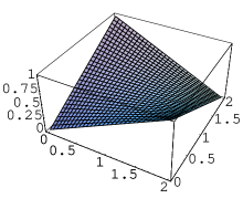
Figure 1: The ruled₁ surface (r=1,d=2). The horizontal plane is expanded by $y,z$ and the height is $x$.

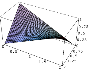
Figure 2: The ruled₂ surface (r=2,d=1). The horizontal plane is expanded by $x,y$ and the height is $z$.

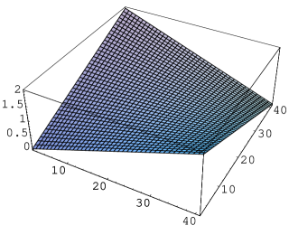
Figure 3: The numerically fitted ruled₁ surface (r=1,d=2).

For a surface to be minimal, its mean curvature vanishes everywhere [1]. The expression for the mean curvature, calculated using eq.(2) of our bilinear interpolation is

$$\frac{-2dr(1-2u)(1-2v)}{[r^{2}+r^{2}(1-2u)^{2}+d^{2}(1-2v)^{2}]^{3/2}}.$$ (16)

for the ruled₁ and

$$\frac{-2r^{3}(1-2u)(1-2v)}{d[d^{2}+r^{2}(1-2u)^{2}+r^{2}(1-2v)^{2}]^{3/2}}.$$ (17)

for the ruled₂.

The mean curvature for the surface is zero only for the $u=\frac{1}{2}$ line and the $v=\frac{1}{2}$ line, whereas for a minimal surface this should be zero for all values of $u$ and $v$.

4 The Numerical Work:

The solution of the Plateau problem was formulated by Courant[2] as minimization of the Dirichlet integral

$$E_{D}(u)=\frac{1}{2}\int_{\Omega}|\nabla u|^{2}$$

where $|\nabla u|^{2}={\rm tr}(^{t}\partial u\partial u)$, where $\partial u$ is the matrix of partial derivatives of u in an orthonormal basis. In [13], a mapping to the conjugate minimal surface was considered in the minimization process. In [9], a diffeomorphism $u_{0}:\Omega\to{\bf R}^{3}$, where $\Omega\subset{\bf R}^{2}$, $u_{0}(\Omega)\subset S(0)$ and maps $u(\cdot,t):\Omega\to{\bf R}^{3},(t>0)$, which satisfies

$$\frac{\partial u}{\partial t}-\Delta_{S(t)}u=0\quad{\rm in}\Omega\times(0,T)$$

with appropriate Dirichlet boundary condition was considered.

In [8], more direct minimization of the numerator of the mean curvature $H$ using parallel computer was performed. In the generalized Newton’s method, the minimization of $F(z)$ of eq.(6) is achieved by the iteration

$$z^{k+1}=z^{k}-DF(z^{k})^{-1}[F(z^{k})],$$ (18)

where $DF(z^{k})^{-1}$ is the inverse of the functional derivative that satisfies

$$DF(z^{k})[z^{k+1}-z^{k}]=-F(z^{k}).$$ (19)

We consider $(N+1)\times(N+1)$ lattice grid points $(u_{i},v_{j})$, $(0\leq i\leq N,0\leq j\leq N)$ and corresponding $z(u_{i},v_{j})$. We keep same number of grid points independent of $r$ and $d$. In the discretized system $z^{k+1}(u_{i},v_{j})$ is defined from $z^{k}(u_{i},v_{j})$ by adding $dz^{k+1}(u_{i},v_{j})$ which can be calculated by solving the linear equation expressed by a matrix $C$ defined by the first and the second fundamental form as

$$Cadz^{k+1}(u,v)=-F(z^{k}(u,v))$$ (20)

Businger et. al. [8] gave a Mathematica code to define the matrix $C$. In our problem of improving the surface starting from the bilinear area, the discretization error in the replacement like

$$\frac{\partial z}{\partial u}=\frac{z(u_{i+1},v_{j})-z(u_{i},v_{j})}{du}$$ (21)

is large and the convergence was poor.

The reason would be lack of explicit third order polynomial term in the evaluation of $dz^{k+1}$ in the numerical methods which manifests itself in the fact that $C_{(i-1,j)}$ and $C_{(i+1,j)}$ are identical. Thus we evaluate the first and second fundamental form on the discretized system by using the Chebyshev polynomial expansion [6].

4.1 Chebyshev Polynomial Expansion

The Chebyshev polynomial of degree $n$ is denoted $T_{n}(x)$ and is given by

$$T_{n}(x)=\cos(n\cos^{-1}x)$$ (22)

where the range of $x$ is $[-1,1]$ and their explicit expressions are given by the recursion

$$T_{0}(x)=1,\quad T_{n+1}(x)=2xT_{n}(x)-T_{n-1}(x)\quad(n\geq 1)$$ (23)

The zeros of $T_{n}(x)$ are located at

$$x_{k}=\cos(\frac{\pi(k+1/2)}{n}),\quad(k=0,1,\cdots,n-1)$$ (24)

If $x_{k}$ $(k=0,1,\cdots,m-1)$ are the $m$ zeros of $T_{m}(x)$, the Chebyshev polynomial satisfies the discrete orthogonality relation for $i,j<m$,

$$\sum_{k=0}^{m-1}T_{i}(x_{k})T_{j}(x_{k})=\left\{\begin{array}[]{ll}0&i\neq j\\ m/2&i=j\neq 0\\ m&i=j=0\end{array}\right.$$ (25)

We first map $z(u_{i},v_{j}),(0\leq u_{i}\leq 1,0\leq v_{j}\leq 1)$ onto $z(x_{i},y_{j}),(-1\leq x_{i}\leq 1,-1\leq y_{j}\leq 1)$ and interpolate values at zeros of the $T_{N+1}(x)$ defined as $x_{l}$ $(l=0,1,\cdots,N)$ and $T_{N+1}(y)$ defined as $y_{m}$, $(m=0,1,\cdots,N)$, i.e. $z(x_{l},y_{m})$.

We define $c(x_{l},n)$ $(n=0,\cdots,N)$ as

$$c(x_{l},n)=\frac{2}{N+1}\sum_{m=1}^{N+1}z(x_{l},y_{m})T_{n}(y_{m})$$ (26)

and interpolate at $y=y_{j}$ via

$$\hat{z}(x_{l},y_{j})=\sum_{n}c(x_{l},n)T_{n}(y_{j})-\frac{1}{2}c(x_{l},0)$$ (27)

Partial derivative in $y$ is performed by replacing $T_{n}(y)$ by

$$\frac{dT_{n}(y)}{dy}=T_{n}^{\prime}(y)\partial_{y}\hat{z}(x_{l},y_{j})=\sum_{n}c(x_{l},n)T_{n}^{\prime}(y_{j}).$$ (28)

So far the $x$-coordinate is restricted to zero points $x^{l}$. Now, interpolation to $x=x_{i}$ is performed by

$$\tilde{c}(n,y_{j})=\frac{2}{N+1}\sum_{l=1}^{N+1}\hat{z}(x_{l},y_{j})T_{n}(x_{l})$$ (29)

We define also $\partial_{y}\tilde{c}(n,y_{j})$ as

$$\partial_{y}\tilde{c}(n,y_{j})=\frac{2}{N+1}\sum_{l=1}^{N+1}\partial_{y}\hat{z}(x_{l},y_{j})T_{n}^{\prime}(x_{l})$$ (30)

The values on the mesh points $\tilde{z}(x_{i},y_{j})$ are

$$\tilde{z}(x_{i},y_{j})=\sum_{n}\tilde{c}(n,y_{j})T_{n}(x_{i})-\frac{1}{2}\tilde{c}(0,y_{j})$$ (31)

and the derivatives $\partial_{x}\tilde{z}(x_{i},y_{j})$ and $\partial_{x}^{2}\tilde{z}(x_{i},y_{j})$ are

$$\partial_{x}\tilde{z}(x_{i},y_{j})=\sum_{n}\tilde{c}(n,y_{j})T_{n}^{\prime}(x_{i})$$ (32)

$$\partial_{x}^{2}\tilde{z}(x_{i},y_{j})=\sum_{n}\tilde{c}(n,y_{j})T_{n}^{\prime\prime}(x_{i})$$ (33)

$$\partial_{x}\partial_{y}\tilde{z}(x_{i},y_{j})=\sum_{n}\partial_{y}\tilde{c}(n,y_{j})T_{n}^{\prime}(x_{i})$$ (34)

In the linear equation

$${Cdz^{k+1}}_{(i,j)}=b_{(i,j)}$$ (35)

the matrix $C$ in the left-hand side(lhs) is a sparse matrix that contains at least nine non-vanishing elements in each row. Around the position ${(i,j)}$ $(0\leq i\leq N,0\leq j\leq N)$ the elements for the nine nearest neighbors of $(i,j)$ are

$$C_{(i-1,j-1)} = -\partial_{y}\tilde{z}(x_{i},y_{j})\cdot\partial_{x}\tilde{z}(x_{i},y_{j})/(2.\cdot du\cdot dv)$$

$$C_{(i-1,j)} = (1+\partial_{y}\tilde{z}(x_{i},y_{j})^{2})/du^{2}-\partial_{y}^{2}\tilde{z}(x_{i},y_{j})\cdot\partial_{x}\tilde{z}(x_{i},y_{j})/du$$

$$C_{(i-1,j+1)} = \partial_{y}\tilde{z}(x_{i},y_{j})\cdot\partial_{x}\tilde{z}(x_{i},y_{j})/(2\cdot du\cdot dv)$$

$$C_{(i,j-1)} = (1+\partial_{x}\tilde{z}(x_{i},y_{j})^{2})/dv^{2}+\partial_{x}\tilde{z}(x_{i},y_{j})\cdot\partial_{x}\partial_{y}\tilde{z}(x_{i},y_{j})/dv$$

$$-\partial_{y}\tilde{z}(x_{i},y_{j})\cdot\partial_{x}^{2}\tilde{z}(x_{i},y_{j})/dv$$

$$C_{(i,j)} = -2\cdot(1+\partial_{y}\tilde{z}(x_{i},y_{j})^{2})/du^{2}-2\cdot(1+\partial_{x}\tilde{z}(x_{i},y_{j})^{2})/dv^{2}$$

$$C_{(i,j+1)} = (1+\partial_{x}\tilde{z}(x_{i},y_{j})^{2})/dv^{2}-\partial_{x}\tilde{z}(x_{i},y_{j})\cdot\partial_{x}\partial_{y}\tilde{z}(x_{i},y_{j})/dv$$

$$+\partial_{y}\tilde{z}(x_{i},y_{j})\cdot\partial_{x}^{2}\tilde{z}(x_{i},y_{j})/dv$$

$$C_{(i+1,j-1)} = \partial_{y}\tilde{z}(x_{i},y_{j})\cdot\partial_{x}\tilde{z}(x_{i},y_{j})/(2\cdot du\cdot dv)$$

$$C_{(i+1,j)} = (1+\partial_{y}\tilde{z}(x_{i},y_{j})^{2})/du^{2}+\partial_{y}^{2}\tilde{z}(x_{i},y_{j})\cdot\partial_{x}\tilde{z}(x_{i},y_{j})/du$$

$$-\partial_{y}\tilde{z}(x_{i},y_{j})\cdot\partial_{x}\partial_{y}\tilde{z}(x_{i},y_{j})/du$$

$$C_{(i+1,j+1)} = -\partial_{y}\tilde{z}(x_{i},y_{j})\cdot\partial_{x}\tilde{z}(x_{i},y_{j})/(2\cdot du\cdot dv)$$ (36)

The right hand side is

$$b_{(i,j)} = 2\cdot\partial_{x}\tilde{z}(x_{i},y_{j})\cdot\partial_{x}\partial_{y}\tilde{z}(x_{i},y_{j})\cdot\partial_{y}\tilde{z}(x_{i},y_{j})-\partial_{x}^{2}\tilde{z}(x_{i},y_{j})\cdot(1+\partial_{y}\tilde{z}(x_{i},y_{j})^{2})$$ (37)

$$- (1+\partial_{x}\tilde{z}(x_{i},y_{j})^{2})\cdot\partial_{y}^{2}\tilde{z}(x_{i},y_{j})$$

The linear equation

$${Cdz^{k+1}}_{(i,j)}=b_{(i,j)}$$ (38)

for $(N-1)\times(N-1)$ length’s vector corresponding to the points inside the boundary can be solved by using standard computer library.

In the actual numerical calculation we multiply a reduction factor to the solution $dz^{k+1}$ in each step to control the convergence.

4.2 Evaluation of the Area

The standard expression [1] in the differential geometry for the area of a regular surface x$(u,v)$ parameterized in terms of two scalar parameters $u$ and $v$ is

$$\rm{area}=\int\limits du\int\limits dv\,|{\mathbf{x}}_{u}\times{\mathbf{x}}_{v}|,$$ (39)

with

$\displaystyle{\mathbf{x}}_{u}\equiv\frac{\partial\mathbf{x}}{\partial u}$ and $\displaystyle{\mathbf{x}}_{v}\equiv\frac{\partial\mathbf{x}}{\partial v}.$ For $\mathbf{x=x}(x,y,z(x,y)),$ this becomes [1]

$$\rm{area}=\int_{Q}\sqrt{1+z_{x}^{2}+z_{y}^{2}}\,dx\,dy,$$ (40)

where $Q$ is the normal projection of the surface onto the $xy$ plane. Accordingly, we calculated the area formed by the above mentioned discrete points as

$$\sum_{(i,j)}\sqrt{1+\partial_{x}\tilde{z}(x_{i},y_{j})^{2}+\partial_{y}\tilde{z}(x_{i},y_{j})^{2}}du\cdot dv.$$ (41)

This expression contains discretization errors. To estimate that, we discretized the bilinear interpolation for $r=d=1$ in eq.(12) as a $31\times 31$ grid, and calculated the area obtained (of the discrete points) by this eq. (41). This gave 1.2717 i.e. 0.7% underestimation of the exact value 1.280789 obtained by eq.(39).

In Fig.4, we show difference of the numerically calculated (N=40) minimal surface and the ruled₁ surface for $r=d=1$. The corresponding difference of $r=2,d=1$ is shown in Fig.5.

That indicated that before reporting our ‘numerical areas’ we should compare different algorithms for calculating area out of a given set of points. Thus, we calculated the area by the sum of triangle $S_{1}$ spanned by

${\mbox{\boldmath$v$}}_{(i,j)}^{1}=(0,dv,z(u_{i},v_{j})-z(u_{i},v_{j-1}))$ and ${\mbox{\boldmath$v$}}_{(i,j)}^{2}=(du,0,z(u_{i},v_{j})-z(u_{i-1},v_{j}))$, and $S_{2}$ spanned by ${\mbox{\boldmath$v$}}_{(i,j)}^{2}$ and ${\mbox{\boldmath$v$}}_{(i,j)}^{3}=(du,dv,z(u_{i},v_{j})-z(u_{i-1},v_{j-1}))$

$$\sum_{(i,j)}(|{\mbox{\boldmath$v$}}^{1}_{(i,j)}\times{\mbox{\boldmath$v$}}^{2}_{(i,j)}|+|{\mbox{\boldmath$v$}}^{2}_{(i,j)}\times{\mbox{\boldmath$v$}}^{3}_{(i,j)}|)/2$$ (42)

The sum of triangles evaluated by the cross products is 1.281277037,i.e. 0.038% overestimation.

The sum of triangles in the case of N=41 is 1.2811 i.e. 0.02% overestimation and in the case of N=21 is 1.2819 i.e. 0.09%.

We also used a computer algebra system [14] to find the two-dimensional interpolation surface working by fitting polynomial curves between successive data points followed by finding areas of the analytical interpolation surface $\mathbf{x}$ by an exact double integral of eq.(39). The order 2 interpolation gave the above area as 1.280789195, the same up to 7 decimal places as the area without any discretization.

Guided by this check, for areas formed by points we report both the areas calculated by triangulation as well by the interpolation-followed-by-the-double-integral; the numerical values strongly suggest these as better algorithms than the one used in eq.(41).

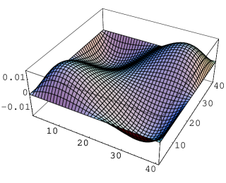
Figure 4: The difference of the numerical minimum and the ruled surface (r=1,d=1).

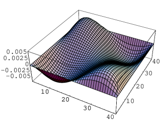
Figure 5: The difference of the numerical minimum and the ruled surface (r=2,d=1).

The area of the ruled surface can be calculated analytically[10]. In the Appendix, we give formulae of the area of the ruled₁ surface and the ruled₂ surface. Numerically calculated area of the minimal surfaces( corresponding to the ruled₂ surface) and analytically calculated area of the ruled surfaces for given $r$ and $d$ are compared in Table.1. The error bars are estimated from the convergence of the iteration. Numerical minimal surfaces corresponding to the ruled₁ are also slightly smaller than the analytical results. In the numerical calculation, approach to the absolute minimum is not guaranteed. In a variational calculation we could obtain slightly smaller area.

$r,d$	numerical area	ruled2 area	ruled1 area
1, 1	1.2793(5)	1.280789275	1.280789275
2, 1	2.3665(5)	2.366974371	1.861564196
1, 2	3.1753(5)	3.180414498	4.316148066
3, 1	3.4916(5)	3.491711893	2.595828045
1, 3	5.9310(5)	5.936348433	9.325179471
3, 2	7.2582(5)	7.259880701	6.208799631
2, 3	8.5226(5)	8.527786411	10.22064879

Table 1: The numerical area (calculated using the order 2 interpolation) and the analytical area of the ruled₂ surface for the hyperbolic paraboloid of given $r$ and $d$. Analytical area of the ruled₁ surface is added for comparison.

An explicit analytical calculation of the minimal surface in ${\bf R}^{3}$ is given in Appendix 2. By constructing the conjugate minimal surface, Karcher[11] transformed the plateau problem in ${\bf R}^{3}$ into that in ${\bf S}^{3}$ and showed that the global Weierstrass representation of triply periodic minimal surfaces is possible. We do not know whether the analytical calculation of the amount of the exact minimal surface area is possible through this method.

We showed in the Appendix B that the exact minimal surface of Schwarz can be visualized. In order to evaluate the area, however, we need to interpolate the analytically obtained coordinates of the surface and perform numerial integration. We leave this task as a future study. Accurate numerical evaluation of the amount of the area is important for physical application and the Chebyschev polynomial expansion is a practical method for performing this process since the area is parametrized as $(x,y,z(x,y)$ instead of $(x(r,\theta),y(r,\theta),z(r,\theta))$.

Appendix A Appendix 1: Area of the ruled surface

In this Appendix, we present the analytical formulae of the area of ruled surfaces[10].

A.1 Ruled₁ surface

In the case of ruled₁ surface we define ${\mbox{\boldmath$r$}}_{12}=(r,d,0)$, ${\mbox{\boldmath$r$}}_{43}=(-r,d,0)$, ${\mbox{\boldmath$r$}}_{23}=(-r,0,d)$, ${\mbox{\boldmath$r$}}_{14}=(r,0,d)$. The area is given by

$$\int_{0}^{1}du\int_{0}^{1}dv|[u{\mbox{\boldmath$r$}}_{12}+(1-u){\mbox{\boldmath$r$}}_{43}]\times[v{\mbox{\boldmath$r$}}_{23}+(1-v){\mbox{\boldmath$r$}}_{14}]|$$ (43)

which becomes

$$\int_{0}^{1}du\int_{0}^{1}dvd\sqrt{d^{2}+2r^{2}(1-2u+2u^{2})-4r^{2}v(1-v)}$$

$$=d[\sqrt{d^{2}+2r^{2}}/3$$

$$-2d^{3}\tan^{-1}\left[\frac{dr(6d^{4}+2d^{2}r^{2}-(4d^{2}+r^{2})r\sqrt{d^{2}+2r^{2}})}{-4d^{6}+4d^{2}r^{4}+r^{6}}\right]/(12r^{2})$$

$$+2d^{3}\tan^{-1}\left[\frac{dr(6d^{4}+2d^{2}r^{2}+(4d^{2}+r^{2})r\sqrt{d^{2}+2r^{2}})}{-4d^{6}+4d^{2}r^{4}+r^{6}}\right]/(12r^{2})$$

$$-\frac{3d^{2}+r^{2}}{6r}\log\left|\frac{-r+\sqrt{d^{2}+2r^{2}}}{r+\sqrt{d^{2}+2r^{2}}}\right|]$$

$$=d\left[\sqrt{d^{2}+2r^{2}}/3+d^{3}\tan^{-1}[\frac{2r^{2}d\sqrt{d^{2}+2r^{2}}}{r^{4}-2r^{2}d^{2}-d^{4}}]/(6r^{2})\right.$$

$$\left.-\frac{3d^{2}+r^{2}}{6r}\log\left|\frac{-r+\sqrt{d^{2}+2r^{2}}}{r+\sqrt{d^{2}+2r^{2}}}\right|\right].$$ (44)

A.2 Ruled₂ surface

The ruled₂ surface is characterized by ${\mbox{\boldmath$r$}}_{13}=(0,d,d)$, ${\mbox{\boldmath$r$}}_{42}=(0,d,-d)$, ${\mbox{\boldmath$r$}}_{23}=(-r,0,d)$, ${\mbox{\boldmath$r$}}_{41}=(-r,0,-d)$. The area is given by

$$\int_{0}^{1}du\int_{0}^{1}dv|[u{\mbox{\boldmath$r$}}_{13}+(1-u){\mbox{\boldmath$r$}}_{42}]\times[v{\mbox{\boldmath$r$}}_{23}+(1-v){\mbox{\boldmath$r$}}_{41}]|$$ (45)

which becomes

$$\int_{0}^{1}du\int_{0}^{1}dvd\sqrt{d^{2}+2r^{2}(1-2u+2u^{2})+d^{2}(1-2v)^{2}}$$

$$=d\sqrt{d^{2}+2r^{2}}/3+\frac{r^{2}}{6}\tan^{-1}[\frac{d\sqrt{d^{2}+2r^{2}}}{r^{2}}]$$

$$+\frac{r^{2}}{3}\log\left|\frac{d+\sqrt{d^{2}+2r^{2}}}{-d+\sqrt{d^{2}+2r^{2}}}\right|+\frac{dr}{4}(1+\frac{d^{2}}{3r^{2}})\log\left|\frac{r+\sqrt{d^{2}+2r^{2}}}{-r+\sqrt{d^{2}+2r^{2}}}\right|.$$ (46)

Appendix B Appendix 2: Visualization of the exact minimal surface

In this Appendix, we construct conformal mapping from a complex $\omega$ plane to the skew quadrilateral of Schwarz, and visualize the surface using Mathematica[14].

The domain of the conformal mapping consists of an area bounded by four singular points $a,b,c$ and $d$, where $\displaystyle a=\frac{-1+\sqrt{3}}{\sqrt{2}}$, $\displaystyle b=\frac{-1+\sqrt{3}}{\sqrt{2}}i$, $\displaystyle c=\frac{1-\sqrt{3}}{\sqrt{2}}$ and $\displaystyle d=\frac{1-\sqrt{3}}{\sqrt{2}}i$[4]. The Schwarz-Christoffel transformation corresponding to the four singular points would be expressed as

$$R(\omega)=f(\omega)[(\omega-a)(\omega-b)(\omega-c)(\omega-d)]^{-1/2}.$$

The Schwarz reflection principle implies, however, rotation of 180^∘ about the boundary straight line is a symmetry of the mapping and the minimal surface area inside the boundary arc can be reflected to outside the boundary arc. Taking into account the presence of conjugate singular points, the actual $R(\omega)$ is expressed as

$$R(\omega)=f(\omega)[(\omega-a)(\omega-b)(\omega-c)(\omega-d)(\omega-a^{\prime})(\omega-b^{\prime})(\omega-c^{\prime})(\omega-d^{\prime})]^{-1/2},$$

where $a^{\prime}=1/b,b^{\prime}=1/c,c^{\prime}=1/d$ and $d^{\prime}=1/a$. The position of the poles in the complex $\omega$ plane are given in Fig.7.

Figure 6: Domains of the area in the complex $\omega$ plane which are mapped to the Schwarz’s minimal surface [4].

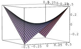
Figure 7: A ruled surface with the same boundary as that of Schwarz’s minimal surface defined in [4].

We transform $\omega$ to $i\rho$, introduce a scaling parameter $\kappa$ and define

$$R(i\rho)=\frac{2i\kappa}{\sqrt{1+14\rho^{4}+\rho^{8}}}.$$

The coordinates of the minimal surface corresponding to the eq.(2) scaled by $\kappa$ become

$$\frac{x}{\kappa}=Re\int^{\rho}\frac{2(1+\rho^{2})}{\sqrt{1+14\rho^{4}+\rho^{8}}}d\rho$$

$$\frac{y}{\kappa}=-Im\int^{\rho}\frac{2(1-\rho^{2})}{\sqrt{1+14\rho^{4}+\rho^{8}}}d\rho$$

$$\frac{z}{\kappa}=Re\int^{\rho}\frac{4\rho}{\sqrt{1+14\rho^{4}+\rho^{8}}}d\rho$$ (47)

The scaling parameter $\kappa$ is defined at the end of the calculation.

The boundary of the domain of the conformal mapping is bounded by four circles like

$$\omega=-\frac{1+i}{\sqrt{2}}+\sqrt{2}e^{i\theta},\quad\frac{\pi}{6}\leq\theta\leq\frac{\pi}{3}.$$

When $\theta$ varies $\frac{\pi}{6}\to\frac{\pi}{3}$, $\omega$ varies from $\frac{-1+\sqrt{3}}{\sqrt{2}}\to\frac{-1+\sqrt{3}}{\sqrt{2}}i$, i.e. $a$ to $b$.

The integral of $x,y,z$ in the Weierstrass-Enneper representation given in sect.2 can be obtained by using the Mathematica,

$$\frac{x}{\kappa}=[2\rho\sqrt{\rho^{4}-4\sqrt{3}+7}\sqrt{\rho^{4}+4\sqrt{3}+7}\left(F_{1}\left(\frac{3}{4};\frac{1}{2},\frac{1}{2};\frac{7}{4};-\frac{\rho^{4}}{7+4\sqrt{3}},\frac{\rho^{4}}{-7+4\sqrt{3}}\right)\rho^{2}\right.$$

$$+\left.3F_{1}\left(\frac{1}{4};\frac{1}{2},\frac{1}{2};\frac{5}{4};-\frac{\rho^{4}}{7+4\sqrt{3}},\frac{\rho^{4}}{-7+4\sqrt{3}}\right)\right)]/{3\sqrt{\rho^{8}+14\rho^{4}+1}}$$ (48)

$$\frac{y}{\kappa}=[-2\rho\sqrt{\rho^{4}-4\sqrt{3}+7}\sqrt{\rho^{4}+4\sqrt{3}+7}\left(\rho^{2}F_{1}\left(\frac{3}{4};\frac{1}{2},\frac{1}{2};\frac{7}{4};-\frac{\rho^{4}}{7+4\sqrt{3}},\frac{\rho^{4}}{-7+4\sqrt{3}}\right)\right.$$

$$-\left.3F_{1}\left(\frac{1}{4};\frac{1}{2},\frac{1}{2};\frac{5}{4};-\frac{\rho^{4}}{7+4\sqrt{3}},\frac{\rho^{4}}{-7+4\sqrt{3}}\right)\right)]/{3\sqrt{\rho^{8}+14\rho^{4}+1}}$$ (49)

$$\frac{z}{\kappa}=-\frac{2i\sqrt{(\rho^{4}+4\sqrt{3}+7)(\rho^{4}-4\sqrt{3}+7)}F\left(i\sinh^{-1}\left(\frac{\rho^{2}}{\sqrt{7+4\sqrt{3}}}\right)|\frac{7+4\sqrt{3}}{7-4\sqrt{3}}\right)}{\sqrt{(\rho^{8}+14\rho^{4}+1)(7-4\sqrt{3})}}.$$

where $F_{1}(a;b_{1},b_{2};c;x,y)$ is the Appell’s 1st hypergeometric function, $F(\phi,m)$ is the elliptic integral of the first kind.

B.1 The case of mapping inside the circle $\displaystyle\omega=\frac{1-i}{\sqrt{2}}+\sqrt{2}e^{i\theta}$

The boundary of a circle whose center is at $\displaystyle\frac{1-i}{\sqrt{2}}$ in the $\omega$ plane ($\omega=re^{i\alpha}$) is given by

$$\frac{1-i}{\sqrt{2}}+\sqrt{2}(\cos\theta+i\sin\theta)=r(\cos\alpha+i\sin\alpha)$$ (51)

We consider an area where $\alpha$ satisfies $0\leq\alpha\leq\pi/2$. The equation

$$\cot\alpha=\frac{1+2\cos\theta}{-1+2\sin\theta},\quad r=\sqrt{3+2\cos\theta-2\sin\theta}$$ (52)

gives a solution of $\theta$ as

$$\theta(\cot\alpha)=\pm\cos^{-1}\frac{1}{2}[(-1-\cot\alpha+\frac{\cot^{2}\alpha+\cot^{3}\alpha}{1+\cot^{2}\alpha}\mp\frac{\cot\alpha\sqrt{3-2\cot\alpha+3\cot^{2}\alpha}}{1+\cot^{2}\alpha})]$$ (53)

Here we choose the first sign + and the second sign - in the eq.(53). Then the $r_{max}^{2}(\cot\alpha)={3+2\cos[\theta(\cot\alpha)]-2\sin[\theta(\cot\alpha)]}$ as a function of $\cot\alpha$ behaves as Fig.9. There is a branch point at $\cot\alpha=1$, i.e.$\alpha=\pi/4$.

A mapping of a region $0\leq\theta\leq\pi/2$ and $0\leq r\leq\sqrt{3+2\cos\theta-2\sin\theta}$ via

$$\frac{x}{\kappa}=-Re\int^{\rho}\frac{2(1+\rho^{2})}{\sqrt{1+14\rho^{4}+\rho^{8}}}d\rho$$

$$\frac{y}{\kappa}=-Im\int^{\rho}\frac{2(1-\rho^{2})}{\sqrt{1+14\rho^{4}+\rho^{8}}}d\rho$$

$$\frac{z}{\kappa}=Re\int^{\rho}\frac{4\rho}{\sqrt{1+14\rho^{4}+\rho^{8}}}d\rho$$ (54)

is shown in Fig.9. Due to the branch point near $\alpha=\pi/4$, there appears numerical errors represented by thorns emanating from the saddle point. The blank area between the thorn going from the saddle point downwards and the left border of the minimal surface is due to numerical difficulties that inhibit simple extension of $\theta$ and $r$ to their boundaries.

Figure 8: The maximal radius $r_{max}$ squared as a function of ${\cot}\alpha$. In the calculation of the area, the region $0\leq{\cot}\alpha$ is used.

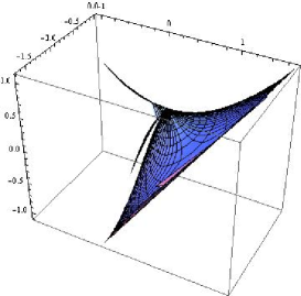
Figure 9: A piece of the Schwarz’s minimal surface. (The front right piece of the minimal surface of Fig. B.2.)

B.2 The case of mapping inside the circle $\displaystyle\omega=\frac{1-i}{\sqrt{2}}+\sqrt{2}e^{i(\theta+\pi/2)}$

The boundary of the area of a circle whose center is at $\displaystyle\frac{1-i}{\sqrt{2}}$ is given by

$$\frac{1-i}{\sqrt{2}}+\sqrt{2}(\cos(\theta+\pi/2)+i\sin(\theta+\pi/2))=r(\cos\alpha+i\sin\alpha)$$ (55)

The equation

$$\tan\alpha=\frac{1+2\cos(\theta+\pi/2)}{-1+\sin(\theta+\pi/2)}=\frac{1-2\sin\theta}{-1+2\cos\theta},r=\sqrt{3-2\cos\theta-2\sin\theta}$$ (56)

gives a solution of $\theta$ as

$$\theta(\tan\alpha)=\pm\cos^{-1}\frac{1}{2}[(1-\tan\alpha-\frac{\tan^{2}\alpha-\tan^{3}\alpha}{1+\tan^{2}\alpha}\mp\frac{\tan\alpha\sqrt{3+2\tan\alpha+3\tan^{2}\alpha}}{1+\tan^{2}\alpha})]$$ (57)

Here we choose both the first and the second sign + in the eq.(57). The $r_{max}(\tan\alpha)$ squared as a function of $\tan\alpha$ is shown in Fig.11.

A mapping of a region $-\pi/2\leq\theta\leq 0$ and $0\leq r\leq\sqrt{3-2\cos\theta-2\sin\theta}$ via

$$\frac{x}{\kappa}=-Re\int^{\rho}\frac{2(1+\rho^{2})}{\sqrt{1+14\rho^{4}+\rho^{8}}}d\rho$$

$$\frac{y}{\kappa}=-Im\int^{\rho}\frac{2(1-\rho^{2})}{\sqrt{1+14\rho^{4}+\rho^{8}}}d\rho$$

$$\frac{z}{\kappa}=Re\int^{\rho}\frac{4\rho}{\sqrt{1+14\rho^{4}+\rho^{8}}}d\rho$$ (58)

is shown in Fig.11, which gives a part of the minimal surface. There appears a missing region in upper left corner due to the singularity of $\tan\alpha$ near $\alpha=90^{\circ}$. The small missing region is mapped in a place rotated by $90^{\circ}$ and $z<-2\times 0.47196$ region as shown in Fig.13.

To evaluate the area of the minimal surface, we use data of the right half of the triangle of Fig.13.

Figure 10: The maximal radius $r_{max}$ squared as a function of $\tan\alpha$. In the calulation of the area, the region $\tan\alpha<0$ is used.

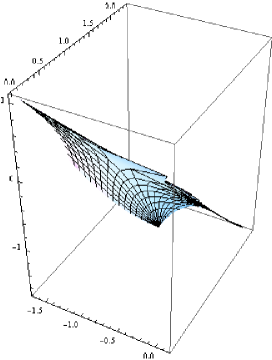
Figure 11: A piece of the Schwarz’s minimal surface (The front left piece of the minimal surface of Fig. B.2. )

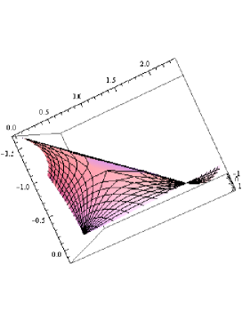
Figure 12: The bird’s eye view of the minimal surface of Fig.11. The missing corner region in that figure appears in the $90^{\circ}$ rotated region.

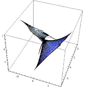
Figure 13: A combination of the two pieces of the Schwarz’s minimal surface.

A combination of the Figs.9 and 11 are shown in Fig.13. The scale parameter $\kappa$ is defined by the height of the $z-$coordinate of the edge of the tetrahedron

$$\int_{0}^{(\sqrt{3}-1)i/\sqrt{2}}\frac{4\rho}{\sqrt{1+14\rho^{4}+\rho^{8}}}d\rho$$

$$=-2i\left(2+\sqrt{3}\right)F\left(-i\sinh^{-1}\left(7-4\sqrt{3}\right)|97+56\sqrt{3}\right)=-0.47196$$ (59)

The Fig.13 indicates that the actual height of the $z-$ coordinate is twice of this value and since this height should be $\displaystyle\frac{1}{2\sqrt{2}}$, $\displaystyle\kappa=\frac{1}{2\sqrt{2}}/(2\times 0.47196)=0.37456$.

We observe that the scale factor given in Ref.[4] does not agree with ours. To the best of our knowledge, it is the first explicit calculation of the exact minimal surface whose bounding contour is the skew quadrilateral.

References

• [1] M. Do Carmo, Differential Geometry of Curves and Surfaces, Prentice Hall, 1976.
• [2] R. Courant, Dirichlet’s Principle, Conformal Mapping, and Minimal Surfaces, Springer, New York, Reprint (1977).
• [3] G. Farin, Curves and Surfaces for Computer Aided Geometric Design 4th ed., Academic Press, 1996.
• [4] J.C.C. Nitche, Lectures on Minimal Surfaces, Cambridge University Press, 1989.
• [5] R. Osserman, A Survey of Minimal Surfaces, Dover Phoenix Editions, Mineola, New York, 1969.
• [6] W.H. Press et al., in Numerical Recipes in C++, Cambridge Univ. Press, 2002
• [7] H.A. Schwarz, Gesammelte mathematische Abhandlungen, 2 vols, Springer, Berlin, 1890.
• [8] W. Businger, P.-A. Chevalier, N. Droux and W. Hett, Mathematica Journal, 4(1994) 70.
• [9] G. Dziuk, An algorithm for evolutionary surfaces, Numer. Math. 58(1991) 603.
• [10] S. Furui, A.M. Green and B. Masud, An Analysis of Four-quark Energies in SU(2) Lattice Monte Carlo based on the Cubic Symmetry, Nucl. Phys. A582 682 (1995).
• [11] H. Karcher, The Triply Periodic Minimal Surfaces of A. Schoen and their Constant Mean Curvature Compagnions, Man. Math. 64, 291 (1989).
• [12] F. J. Lopez and F. Marin, Complete minimal surfaces in $R^{3}$, Publicacions Matemàtiques, Vol. 43 (1999) 341-449.
• [13] U. Pinkall and K. Polthier, Computing Discrete Minimal Surfaces and their Conjugates, Experim. Math., 2(1993) 15.
• [14] The software ”Mathematica” ver. 5.2 & 6(Prerelease), developed by the Wolfram research.