Exact Results for the Ionization of a Model Quantum System

Abstract

We prove that a model atom having one bound state will be fully ionized by a time periodic potential of arbitrary strength $r$ and frequency $\omega$. Starting with the system in the bound state, the survival probability is for small $r$ given by $e^{-\Gamma t}$ for times of order $\Gamma^{-1}$ $\sim r^{-2n}$, where $n$ is the minimum number of “photons” required for ionization (with large modifications at resonances). For late times the decay is like $t^{-3}$ with the power law modulated by oscillations. As $r$ increases the time over which there is exponential decay becomes shorter and the power law behavior starts earlier. Results are for a parametrically excited one dimensional system with zero range potential but comparison with analytical works and with experiments indicate that many features are general.

PACS: 32.80 Rm, 03.65 Bz, 32.80 Wr.

*******

1 Introduction

The solution of the Schrödinger equation with a time dependent potential leading to transitions between bound and free states of a quantum system is clearly of great theoretical and practical interest. Fermi’s golden rule (based on a deep physical interpretation of first order perturbation theory) gives the decay exponent of the survival probability for a system in a bound state subjected to a weak external oscillating potential, with frequency $\omega>\omega_{0}=-u_{b}/\hbar$, $u_{b}$ the energy of the bound state [1]. The approaches used to go beyond the golden rule include higher order perturbation theory, semi-classical phase-space analysis, Floquet theory, complex dilation, exact results for small fields, and numerical integration of the time dependent Schrödinger equation [1]-[16]. These works have yielded both theoretical understanding and good agreement with dissociation experiments in strong laser fields. In particular they have been very successful in elucidating much of the rich structure found in the experiments on the multiphoton ionization of Rydberg atoms by microwave fields [2]–[6]. Explicit results for realistic systems require, of course, the use of some approximations whose reliability is not easy to establish a priori.

It would clearly be desirable to have examples for which one could compute the time evolution of an initially bound state and thus the ionization probability for all values of the frequency and strength of the oscillating potential to as high accuracy as desired without any uncontrolled approximations. This is the motivation for the present work which describes new exact results relating to ionization of a very simple model atom by an oscillating field (potential) of arbitrary strength and frequency. While our results hold for arbitrary strength perturbations, the predictions are particularly explicit and sharp in the case where the strength of the oscillating field is small relative to the binding potential—a situation commonly encountered in practice. Going beyond perturbation theory we rigorously prove the existence of a well defined exponential decay regime which is followed, for late times when the survival probability is already very low, by a power law decay. This is true no matter how small the frequency. The times required for ionization are however very dependent on the perturbing frequency. For a harmonic perturbation with frequency $\omega$ the logarithm of the ionization time grows like $r^{-2n}$, where $r$ is the normalized strength of the perturbation and $n$ is the number of “photons” required for ionization. This is consistent with conclusions drawn from perturbation theory and other methods (the approach in [8] being the closest to ours), but is, as far as we know, the first exact result in this direction. We also obtain, via controlled schemes, such as continued fractions and convergent series expansions, results for strong perturbing potentials.

Quite surprisingly our results reproduce many features of the experimental curves for the multiphoton ionization of excited hydrogen atoms by a microwave field [3]. These features include both the general dependence of the ionization probabilities on field strength as well as the increase in the life time of the bound state when $-n\hbar\omega$, $n$ integer, is very close to the binding energy. Such “resonance stabilization” is a striking feature of the Rydberg level ionization curves [3]. These successes and comparisons with analytical results [1]-[11] suggest that the simple model we shall now describe contains many of the essential ingredients of the ionization process in real systems.

1.1 Description of the model

The unperturbed Hamiltonian in our model is,

$$H_{0}=-{\frac{\hbar^{2}}{2m}}{\frac{d^{2}}{dy^{2}}}-g\delta(y),\ g>0,\ \ -\infty<y<\infty.$$ (1)

$H_{0}$ has a single bound state $u_{b}(y)=\sqrt{p_{0}}e^{-p_{0}|y|},\ p_{0}=\frac{m}{\hbar^{2}}g$ with energy $-\hbar\omega_{0}=-\hbar^{2}p_{0}^{2}/2m$ and a continuous uniform spectrum on the positive real line, with generalized eigenfunctions

$$u(k,y)=\frac{1}{\sqrt{2\pi}}\left(e^{iky}-\frac{p_{0}}{p_{0}+i|k|}e^{i|ky|}\right),\ \ -\infty<k<\infty$$

and energies $\hbar^{2}k^{2}/2m$.

Beginning at some initial time, say $t=0$, we apply a parametric perturbing potential $-g\eta(t)\delta(y)$, i.e.  we change the parameter $g$ in $H_{0}$ to $g(1+\eta(t))$ and solve the time dependent Schrödinger equation for $\psi(y,t)$,

$$\psi(y,t)=\theta(t)u_{b}(y)e^{i\omega_{0}t}+\int_{-\infty}^{\infty}\Theta(k,t)u(k,y)e^{-i\frac{\hbar k^{2}}{2m}t}dk\ \ (t\geq 0)$$ (2)

with initial values $\theta(0)=1,\ \Theta(k,0)=0$. This gives the survival probability $|\theta(t)|^{2}$, as well as the fraction of ejected electrons $|\Theta(k,t)|^{2}dk$ with (quasi-) momentum in the interval $dk$.

This problem can be reduced to the solution of an integral equation [17]. Setting

$$\displaystyle\theta(t)=1+2i\int_{0}^{t}Y(s)ds$$ (3)

$$\displaystyle\Theta(k,t)=\frac{2|k|}{\sqrt{2\pi}(1-i|k|)}\int_{0}^{t}Y(s)e^{i(1+k^{2})s}ds$$ (4)

$Y(t)$ satisfies the integral equation

$$Y(t)=\eta(t)\left\{1+\int_{0}^{t}[2i+M(t-t^{\prime})]Y(t^{\prime})dt^{\prime}\right\}$$ (5)

where we have set $p_{0}=\omega_{0}=\hbar=2m=\frac{g}{2}=1$ and

$$M(s)=\frac{2i}{\pi}\int_{0}^{\infty}\frac{u^{2}e^{-is(1+u^{2})}}{1+u^{2}}du=\frac{1}{2}\sqrt{\frac{i}{\pi}}\int_{s}^{\infty}\frac{e^{-iu}}{u^{3/2}}du.$$

2 Results

Our first exact result is the following: When $\eta(t)$ is a trigonometric polynomial,

$$\eta(t)=\sum_{j=1}^{n}[A_{j}\sin(j\omega t)+B_{j}\cos(j\omega t)],$$ (6)

the survival probability $|\theta(t)|^{2}$ tends to zero as $t\rightarrow\infty$, for all $\omega>0$. That is there will be full ionization for arbitrary strength and frequency of the oscillating field.

Since the main features of the argument are already present in the simplest case $\eta=r\sin(\omega t)$ we now specialize to this case. The asymptotics of $Y(t)$ are obtained from its Laplace transform $y(p)=\int^{\infty}_{0}e^{-pt}Y(t)dt$, which satisfies the functional equation (cf. (5))

$$y(p)=\frac{ir}{2}\left\{{\frac{y(p+i\omega)}{\sqrt{1-ip+\omega}-1}}-{\frac{y(p-i\omega)}{\sqrt{1-ip-\omega}-1}}\right\}+{\frac{r\omega}{\omega^{2}+p^{2}}}$$ (7)

with the boundary condition $y(p)\rightarrow 0$ as $\Im(p)\rightarrow\pm\infty$ (the relevant branch of the square root is $(1-ip-\omega)^{1/2}=-i(\omega-1+ip)^{1/2}$ for $\omega>1$). We show that the solution of (7) with the given boundary conditions is unique and analytic for $\Re(p)>0$, and its only singularities on the imaginary axis are square-root branch points. This in turn implies that $|Y(t)|$ does indeed decay in an integrable way.

The ideas of the proof carry through directly to the more general periodic potential (6) and we have obtained analogous results for a two delta functions reference potential [18].

Full ionization is in fact expected (for entropic reasons) to hold generically, but has, as far as we know, only been proven before for small amplitude of the oscillating potential with $\omega>1$ ([10], [11]), or for sufficiently random perturbations ([10]).

The detailed behavior of the system as a function of $t$, $\omega$, and $r$ is obtained from a precise study of the singularities of $y(p)$ in the whole complex $p$-plane. Here we discuss them for small $r$; below, the symbol $\varepsilon$ describes error bounds of order $O(r^{2-\delta}),\frac{1}{2}<\delta<1$. At $p=\{in\omega-i:n\in\bf{Z}\}$, $y$ has square root branch points and $y$ is analytic in the right half plane and also in an open neighborhood ${\cal{N}}$ of the imaginary axis with cuts through the branch points. As $|\Im(p)|\rightarrow\infty$ in ${\cal{N}}$ we have $|y(p)|=O(r\omega|p|^{-2})$. If $|\omega-\frac{1}{n}|>C_{n}\varepsilon,\,n\in\bf{Z}^{+}$, for some constants $C_{n}$, then for small $r$ the function $y$ has a unique pole $p_{m}$ in each of the strips $-m\omega>\Im(p)+1\pm\varepsilon>-m\omega-\omega,\,\ m\in\bf{Z}$. $\Re(p_{m})$ is strictly independent of $m$ and gives the exponential decay of $\theta$.

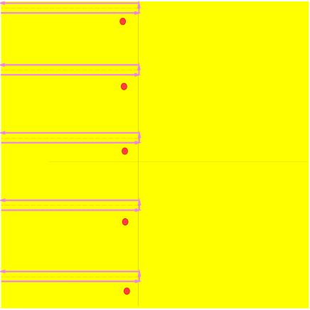
Figure 1: Singularities of $y$ and relevant inverse Laplace contours.

The analytic structure of $y$ is indicated in Figure 1 where the dotted lines represent (the square root) branch cuts and the dark circles are simple poles. The function $Y$ is the inverse Laplace transform of $y$

$$Y(t)=\frac{1}{{2\pi i}}~{}\int_{{\mathcal{C}}}e^{pt}y(p)~{}dp$$ (8)

where the contour of integration ${\mathcal{C}}$ can be initially taken to be the imaginary axis $i\bf{R}$, since $y$ is continuous there and decays like $p^{-2}$ for large $p$.

We then show that $\mathcal{C}$ can be pushed through the poles, collecting the appropriate residues, and along the branch cuts as shown in Figure 1. The residue at the pole $p_{m}$ is proportional to $e^{(p_{0}+im\omega)t}$ while the (rapidly convergent) integral along the $m-$th branch cut is (as seen by standard Laplace integral techniques), a function whose large $t$ behavior is $K_{m}e^{im\omega t}t^{-3/2}$ (the $-3/2$ power comes from the fact that $y$ has square root branch points; $K_{m}$ is some constant).

A detailed analysis along these lines yields ([18], [19]),

$$\theta(t)=e^{-\gamma(r;\omega)t}F_{\omega}(t)+\sum_{m=-\infty}^{\infty}e^{(mi\omega-i)t}h_{m}(t)$$ (9)

where $F_{\omega}$ is periodic of period $2\pi\omega^{-1}$ and $h_{m}(t)\sim\sum_{j=0}^{\infty}c_{m,j}t^{-3/2-j}$ for large $t$ in more than a half plane centered on the positive real half-line. Not too close to resonances, i.e. when $|\omega-n^{-1}|>\varepsilon$, for all integer $n$, $|F_{\omega}(t)|=1+O(r^{2})$ and its Fourier coefficients decay faster than $r^{|2m|}|m|^{-|m|/2}$. Also, the sum in (9) does not exceed $O(r^{2}t^{-3/2})$ for large $t$, and the $h_{m}$ decrease with $m$ faster than $r^{|m|}$.

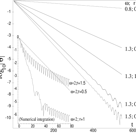
Figure 2: Plot of $\log_{10}|\theta(t)|^{2}$ vs. time in units of $\omega_{0}^{-1}$ for several values of $\omega$ and $r$. The main graph was calculated from (8) and the inset used numerical integration of (5).

By (9), for times of order $1/\Gamma$ where $\Gamma=2\Re(\gamma)$, the survival probability for $\omega$ not close to a resonance decays as $\exp(-\Gamma t)$. This is illustrated in Figure 2 where it is seen that for $r^{<}\hskip-6.45831pt_{\sim}0.5$ the exponential decay holds up to times at which the survival probability is extremely small. Note also the slow decay for $\omega=.8$, when ionization requires the absorption of two photons. For even larger $r$ one can note in the figure oscillatory behavior. This is expected from equation (9).

When $r$ is larger (inset in Fig. 2) the ripples of $|F_{\omega}(t)|$ are visible and the polynomial-oscillatory behavior starts sooner. Since the amplitude of the late asymptotic terms is $O(r^{2})$ for small $r$, increased $r$ can yield a higher late time survival probability. This phenomenon, sometimes referred to as “adiabatic stabilization” [14], [20], can be associated with the perturbation-induced probability of back-transitions to the well.

Using continued fractions $\Gamma$ can be calculated convergently for any $\omega$ and $r$. For small $r$ we have

$$\Gamma\sim\left\{\begin{array}[]{lllllll}\displaystyle\sqrt{\omega-1}\frac{r^{2}}{\omega};&\mbox{\rm if }{\omega}\in(1+\varepsilon,\infty)\\ &\\ \displaystyle\frac{\sqrt{2\omega-1}}{(1-\sqrt{1-\omega})^{2}}\frac{r^{4}}{8\omega};&\mbox{\rm if }{\omega}\in(\frac{1}{2}+\varepsilon,1-\varepsilon)\\ \ldots&\ldots\\ \displaystyle\frac{2^{-2n+2}\sqrt{n\omega-1}}{\displaystyle\prod_{m<n}(1-\sqrt{1-m\omega})^{2}}\frac{r^{2n}}{n\omega};&\mbox{\rm if }{\omega}\in(\frac{1}{n}+\varepsilon,\frac{1}{n-1}-\varepsilon)\end{array}\right.$$ (10)

Eq. (10) agrees with results of perturbation theory. Thus, for $\omega>1$, $\Gamma$ is given by Fermi’s golden rule [1] since the transition matrix element between the bound state with energy $-1$ and the continuum state with energy $k^{2}$ is

$$\big{|}<u_{b}(y)|\delta(y)u(k,y)>\big{|}^{2}=\frac{1}{2\pi}\frac{k^{2}}{1+k^{2}}$$ (11)

while the density of states is ${\frac{2\pi}{k}}$.

The behavior of $\Gamma$ is different at the resonances $\omega^{-1}\in\bf{N}$. For instance, whereas if $\omega$ is not close to $1$, the scaling of $\Gamma$ implied by (10) is $r^{2}$ when $\omega>1$ and $r^{4}$ when $\frac{1}{2}<\omega<1$, when $\omega-1=r^{2}/\sqrt{2}$ we find

$$\Gamma\sim\Big{(}\frac{2^{1/4}}{8}-\frac{2^{3/4}}{16}\Big{)}r^{3}$$

In Figure 3 we plot the behavior of $\Gamma^{-1}$, as a function of $\omega$, for a small value of $r$. The curve is made up of smooth (roughly self-similar) pieces for $\omega$ in the intervals $(n^{-1},(n-1)^{-1})$ corresponding to ionization by $n$ photons.

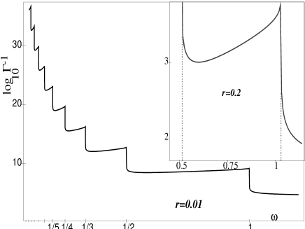
Figure 3: $\log_{10}\Gamma^{-1}$ as a function of $\omega/\omega_{0}$ at $r=0.01$. At $r=0.2$ (inset) shift of the resonance is visible. In the inset the continued fraction was used, while for the main figure the data was extrapolated from (10).

At resonances (for small $r$ these occur for $\omega^{-1}$ close to an integer), the coefficient of $r^{2n}$, the leading term in $\Gamma$, goes to zero. This yields an enhanced stability of the bound state against ionization by perturbations with such frequencies. The origin of this behavior is, in our $d=1$ model, the vanishing of the matrix element in (11) at $k=0$. This behavior should hold quite generally in $d=3$ where there is a factor $k$ in $\Gamma$ coming from the energy density of states near $k=0$. As $r$ increases these resonances shift in the direction of increased frequency. For small $r$ and $\omega=1$ the shift in the position of the resonance, sometimes called the dynamic Stark effect [1], is about $\frac{r^{2}}{\sqrt{2}}$.

In Figure 4 we plot the strength of the perturbation $r$, required to make $|\theta(t)|^{2}={\frac{1}{2}}$ for a time of about 700 oscillations of the perturbing field, i.e. time is measured in units of $\omega^{-1}$, as a function of $\omega$. Also included in this figure are experimental results taken from Table 1 in [3], see also Figures 13 and 18 there for the ionization of a hydrogen atom by a microwave field for approximately the same number of oscillations. In these still ongoing beautiful series of experiments, [3]–[5], the atom is initially in an excited state with principal quantum number $n_{0}$ ranging from 32 to 90. The “natural frequency” $\omega_{0}$ is there taken to be that of an average transition from $n_{0}$ to $n_{0}\pm 1$, so $\omega_{0}\sim n^{-3}_{0}$. The strength of the microwave field $F$ is then normalized to the strength of the nuclear field in the initial state, which scales like $n^{-4}_{0}$. The plot there is thus of $n^{4}_{0}F$ vs. $n^{3}_{0}\omega$. To compare the results of our model with the experimental ones we had to relate $r$ to $n_{0}^{4}F$, and given the difference between the hydrogen atom perturbed by a polarized electric field $V_{1}=xF\sin(\omega t)$, and our model, this is clearly not something that can be done in a unique way. We therefore simply tried to find a correspondence between $n_{0}^{4}F$ and $r$ which would give the best visual fit. Somewhat to our surprise these fits for different values of $\omega/\omega_{0}$ all turned out to have values of $r$ close to $3n_{0}^{4}F$.

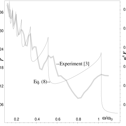
Figure 4: Threshold amplitudes for $50\%$ ionization vs. $\omega/\omega_{0}$, calculated from eq. (10), and in the experiment [3]. In the calculation, the dynamic Stark effect was approximated using an averaged $r$ over the range.

A correspondence of the same order of magnitude is obtained by comparing the perturbation-induced shifts of bound state energies in our model and in hydrogen. We note that the maximal values of $r$ in Figure 4 are still within the regime where only a few terms in (9) are sufficient.

In Figure 5 we plot $|\theta(t)|^{2}$ vs. $r$ for a fixed $t$ and two different values of $\omega$. These frequencies are chosen to correspond to the values of $\omega/\omega_{0}$ in the experimental curves, Figure 1 in [5] and Figure 1b in [3]. The agreement is very good for $\omega/\omega_{0}\approx.1116$ and reasonable for the larger ratio. Our model essentially predicts that when the fields are not too strong, the experimental survival curves for a fixed $n_{0}^{3}\omega$ (away from the resonances) should behave essentially like $\displaystyle\exp\left(-C[n^{4}_{0}F]^{\scriptstyle\frac{\scriptstyle 2}{\scriptstyle n_{0}^{3}\omega}}\,\omega\,t\right)$ with $C$ depending on $n_{0}^{3}\omega$ but, to first approximation, independent of $n_{0}^{4}F$.

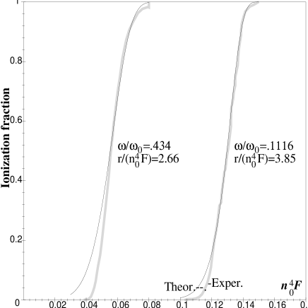
Figure 5: Ionization fraction at fixed $t$ (corresponding to 300 oscillations) as a function of amplitude.

3 Concluding remarks

Given the simplicity of our model, the similarity (using a minimal numbers of adjustable parameters) with the experiments on hydrogen atoms was surprising to us. As already noted these experimental results and in particular the resonances can be understood quite well, including some details, by doing calculations on the full hydrogen atom or a one dimensional version of it [2]-[6]. Still, it is interesting to see that similar structures arise also in very simple models. It suggests that various features of the ionization process have a certain universal character. To really pin down the reason for this universality will require much further work.

We note that for $\omega>\omega_{0}$, in the limit of small amplitudes $r$, a predominantly exponential decay of the survival probability followed by a power-law decay was proved in [11] for three dimensional models with quite general local binding potentials having one bound state, perturbed by $r\cos(\omega t)V(y)$, where $V$ is a local potential. Our results for general $\omega$ and $r$ can be thought of as coming from a rigorous Borel summation of the formal (exponential) asymptotic expansion of $Y$ for $t\rightarrow\infty$. These methods can be extended to other systems [17] including, we hope, realistic ones.

Acknowledgments. We thank A. Soffer, M. Weinstein and P. M. Koch for valuable discussions and for providing us with their papers. We also thank R. Barker, S. Guerin and H. Jauslin for introducing us to the subject. Work of O. C. was supported by NSF Grant 9704968, that of J. L. L. and A. R. by AFOSR Grant F49620-98-1-0207.

costin@math.rutgers.edu lebowitz@sakharov.rutgers.edu rokhlenk@math.rutgers.edu.

References

- [1] Atom-Photon Interactions, by C. Cohen-Tannoudji, J. Duport-Roc and G. Arynberg, Wiley (1992); Multiphoton Ionization of Atoms, S. L. Chin and P.Lambropoulus, editors, Academic Press (1984).
- [2] R. Blümel and U. Similansky, Z. Phys. D6, 83 (1987); G. Casatti and L. Molinari, Prog. Theor. Phys. (Suppl) 98, 286 (1989).
- [3] P. M. Koch and K.A.H. van Leeuwen, Physics Reports 255, 289 (1995).
- [4] J. E. Bayfield et al., Phys. Rev. A53, R12 (1996); P. M. Koch, E. J. Galvez and S. A. Zelazny, Physica D 131, 90 (1999).
- [5] P. M. Koch, Acta Physica Polonica A 93 No. 1, 105–133 (1998).
- [6] A Buchleitner, D. Delande and J.-C. Gay, J. Opt. Soc. B 12, 505 (1995).
- [7] Zero Range Potentials and Their Application in Atomic Physics, Yu. N. Demkov and V. N. Ostrovskii, Plenum (1988).
- [8] S. M. Susskind, S. C. Cowley, and E. J. Valeo, Phys.Rev. A 42, 3090 (1994).
- [9] G. Scharf, K.Sonnenmoser, and W. F. Wreszinski, Phys.Rev. A 44, 3250 (1991); S. Geltman, J. Phys. B: Atom. Molec. Phys. 5, 831 (1977).
- [10] C.-A. Pillet, Comm. Math. Phys. 102, 237 (1985) and 105, 259 (1986); K. Yajima, Comm. Math.Phys. 89, 331 (1982); I. Siegel, Comm. Math. Phys. 153, 297 (1993); W. van Dyk and Y. Nogami, Phys. Rev. Lett. 83, 2867 (1999).
- [11] A. Soffer and M. I. Weinstein, Jour. Stat. Phys. 93, 359–391 (1998).
- [12] A. Maquet, S.-I. Chu and W. P. Reinhardt, Phys. Rev. A 27, 2946 (1983); C. Holt, M. Raymer, and W. P. Reinhardt, Phys. Rev. A 27, 2971 (1983); S.-I. Chu, Adv. Chem. Phys. 73, 2799 (1988); R. M. Potvliege and R. Shakeshaft, Phys. Rev. A 40, 3061 (1989).
- [13] M. Holthaus and B. Just, Phys. Rev. A 49, 1950 (1994); S. Guerin et al., J. Phys. A 30, 7193 (1997); S. Guerin and H.-R. Jauslin, Phys. Rev. A 55, 1262 (1997) and references there.
- [14] A. Fring, V. Kostrykin and R. Schrader, Jour. of Physics B29 (1996 5651; C. Figueira de Morisson Faria, A. Fring and R. Schrader, Jour. of Physics B31 (1998) 449; A. Fring, V. Kostrykin and R. Schrader, Jour. of Physics A30 (1997) 8559; C. Figueira de Morisson Faria, A. Fring and R. Schrader, Analytical treatment of stabilization preprint physics/9808047 v2.
- [15] C. Lefarestier et al., J. Comput. Phys. 94, 59 (1991); C. Ceyan and K. C. Kulander, Comp. Phys. Comm. 63, 529 (1991).
- [16] S. Guerin, Phys. Rev. A 56, 1458 (1997); G. N. Gibson et al., Phys. Rev. Lett. 81, 2663 (1998).
- [17] A. Rokhlenko and J. L. Lebowitz, to appear in JMP, July 2000; Texas 99-187, Los Alamos 9905015.
- [18] O. Costin, J. L. Lebowitz and A. Rokhlenko (in preparation).
- [19] O. Costin, J. L. Lebowitz, A. Rokhlenko, to appear in Proceedings of the CRM meeting “Nonlinear Analysis and Renormalization Group”, American Mathematical Society publications (2000).
- [20] J. R. Vos and M. Gavrila, Phys. Rev. Lett. 68, 170 (1992).