On the self-similar asymptotics for generalized non-linear kinetic Maxwell models

Abstract.

Maxwell models for nonlinear kinetic equations have many applications in physics, dynamics of granular gases, economy, etc. In the present manuscript we consider such models from a very general point of view, including those with arbitrary polynomial non-linearities and in any dimension space. It is shown that the whole class of generalized Maxwell models satisfies properties which one of them can be interpreted as an operator generalization of usual Lipschitz conditions. This property allows to describe in detail a behavior of solutions to the corresponding initial value problem. In particular, we prove in the most general case an existence of self similar solutions and study the convergence, in the sense of probability measures, of dynamically scaled solutions to the Cauchy problem to those self-similar solutions, as time goes to infinity. The properties of these self-similar solutions, leading to non classical equilibrium stable states, are studied in detail. We apply the results to three different specific problems related to the Boltzmann equation (with elastic and inelastic interactions) and show that all physically relevant properties of solutions follow directly from the general theory developed in this paper.

1. Introduction

The classical (elastic) Boltzmann equation with the Maxwell-type interactions is well-studied in literature (see [4, 14] and references therein). Roughly speaking, this is a mathematical model of a rarefied gas with binary collisions such that the collision frequency is independent of the velocities of colliding particles.

Maxwell models of granular gases were introduced relatively recently in [6] (see also [2] for the one dimensional case). Soon after, these models became very popular among people studying granular gases (see, for example, the book [13] and references therein). There are two obvious reasons for this fact. First, the inelastic Maxwell-Boltzmann equation can be essentially simplified by the Fourier transform similarly to the elastic one [5, 6] and second, solutions to the spatially homogeneous inelastic Maxwell-Boltzmann equation have a non-trivial self-similar asymptotics, and, in addition, the corresponding self-similar solution has a power-like tail for large velocities. The latter property was conjectured in [16] and later proved in [8, 9] (see also [3]). It is remarkable that such an asymptotics is absent in the elastic case (roughly speaking, the elastic Boltzmann equation has too many conservation laws). On the other hand, the self-similar asymptotics was proved in the elastic case for initial data with infinite energy [7] by using other mathematical tools compared to [8]. The recently published exact self-similar solutions [10] for elastic Maxwell mixtures (also with power-like tails) definitely suggest the self-similar asymptotics for such elastic systems. Finally we mention recent publications [1, 15, 22] , where one dimensional Maxwell-type models were introduced for applications to economy models and again the self-similar asymptotics and power-like tail were found.

Thus all the above discussed models describe qualitatively different processes in physics or economy, however their solutions have a lot in common from the mathematical point of view. It is also clear that some further generalizations are possible: one can, for example, include in the model multiple (not just binary) interactions still assuming the constant (Maxwell-type) rate of interactions. Will the multi-linear models have similar properties? The answer to this question is affirmative, as we shall see below. It becomes clear that there must be some general mathematical properties of Maxwell models, which, in turn, can explain properties of any particular model. Essentially, there must be just one main theorem, from which one can deduce all the above discussed facts and their possible generalizations. The goal of this paper is to consider Maxwell models from a very general point of view and to establish their key properties that lead to the self-similar asymptotics.

The paper is organized as follows. We introduce in Section 2 three specific Maxwell models of the Boltzmann equation: (A) classical (elastic) Boltzmann equation; (B) the model (A) in the presence of a thermostat; (C) inelastic Boltzmann equation. Then, in Section 3, we perform the Fourier transform and introduce an equation that includes all the three models as particular cases. A further generalization is done in Section 4, where the concept of generalized multi-linear Maxwell model (in the Fourier space) is introduced. Such models and their generalizations are studied in detail in Sections 5-10. The concept of an $L$-Lipschitz nonlinear operator, one of the most important for our approach, is explained in Section 4 (Definition 4.1). It is proved (Theorem 4.2) that all multi-linear Maxwell models satisfy the $L$-Lipschitz condition. This property of the models constitutes a basis for the general theory.

The existence and uniqueness of solutions to the initial value problem is proved in Section 5 (Theorem 5.2). Then we study in Section 6 the large time asymptotics under very general conditions that are fulfilled, in particular, for all our models. It is shown that the $L$-Lipschitz condition leads to self-similar asymptotics provided the corresponding self-similar solution does exist. The existence and uniqueness of self-similar solutions is proved in Section 7 (Theorem 7.1). This result can be considered, to some extent, as the main theorem for general Maxwell-type models. Then, in Section 8, we go back to the multi-linear models of Section 4 and study more specific properties of their self-similar solution. We explain in Section 9 how to use our theory for applications to any specific model: it is shown that the results can be expressed in terms of just one function $\mu(p),p>0,$ that depends on the spectral properties of the specific model.

General properties (positivity, power-like tails, weak convergence of probability measures, etc.) of the self-similar solutions are studied in Section 10. This study also includes the case of one dimensional models, where the Laplace (instead of Fourier) transform is used.

Finally, in Section 11, we establish in the unified statement (Theorem 11.1) the main properties of Maxwell models (A),(B) and (C) of the Boltzmann equation. This result is, in particular, an essential improvement of earlier results of [7] for the model (A) and quite new for the model (B). Applications to one dimensional models are also briefly discussed at the end of Section 11.

2. Maxwell models of the Boltzmann equation

We consider a spatially homogeneous rarefied $d$-dimensional gas $(d=2,3,\ldots)$ of particles having a unit mass. Let $f(v,t)$, where $v\in{\mathbb{R}}^{d}$ and $t\in{\mathbb{R}}_{+}$ denote respectively the velocity and time variables, be a one-particle distribution function with the usual normalization

$$\int_{{\mathbb{R}}^{d}}dv\,f(v,t)=1\ .$$ (2.1)

Then $f(v,t)$ has an obvious meaning of a time-dependent probability density in ${\mathbb{R}}^{d}$. We assume that the collision frequency is independent of the velocities of colliding particles (Maxwell-type interactions) and consider three different physical models (A), (B) and (C) described below.

(A) Classical Maxwell gas (elastic collisions). In this case $f(v,t)$ satisfies the usual Boltzmann equation

$$f_{t}=Q(f,f)=\int_{{\mathbb{R}}^{d}\times S^{d-1}}\mkern-32.0mudw\,d\omega\,g\left(\frac{u\cdot\omega}{|u|}\right)\Big{[}f(v^{\prime})f(w^{\prime})-f(v)f(w)\Big{]}\ ,$$ (2.2)

where the exchange of the velocities after a collision are given by

$$v^{\prime}=\frac{1}{2}(v+w+|u|\omega)\,,\qquad\ \text{and}\ \ \quad w^{\prime}=\frac{1}{2}(v+w-|u|\omega)$$

where $u=v-w$ is the relative velocity and $\Omega\in S^{d-1}$. For the sake of brevity we shall consider below the model non-negative collision kernels $g(s)$ such that $g(s)$ is integrable on $[-1,1]$. The argument $t$ of $f(v,t)$ and similar functions is often omitted below (as in Eq. (2.2)).

(B) Elastic model with a thermostat This case corresponds to model (A) in the presence of a thermostat that consists of Maxwell particles with mass $m>0$ having the Maxwellian distribution

$$M(v)=\left(\frac{2\pi T}{m}\right)^{-d/2}\exp\left(-\frac{m|v|^{2}}{2T}\right)$$ (2.3)

with a constant temperature $T>0$. Then the evolution equation for $f(v,t)$ becomes

$$f_{t}=Q(f,f)+\theta\int dw\,d\omega\,g\left(\frac{u\cdot\omega}{|u|}\right)\Big{[}f(v^{\prime})M(w^{\prime})-f(v)M(w)\Big{]}\ ,$$ (2.4)

where $\theta>0$ is a coupling constant, and the precollision velocities is now

$$v^{\prime}=\frac{v+m(w+|u|\omega)}{1+m},\qquad\ \text{and}\ \ \quad w^{\prime}=\frac{v+mw-|u|\omega}{1+m},$$

with $u=v-w$ the relative velocity and $\omega\in S^{d-1}$.

Equation (2.4) was derived in [10] as a certain limiting case of a binary mixture of weakly interacting Maxwell gases.

(C) Maxwell model for inelastic particles. We consider this model in the form given in [8]. Then the inelastic Boltzmann equation in the weak form reads

$$\frac{\partial}{\partial t}(f,\psi)=\int_{{\mathbb{R}}^{d}\times{\mathbb{R}}^{d}\times S^{d-1}}\mkern-36.0mudv\,dw\,d\omega\,f(v)f(w)\frac{|u\cdot\omega|}{|u|}[\psi(v^{\prime})-\psi(v)]\ ,$$ (2.5)

where $\psi(v)$ is a bounded and continuous test function,

$$(f,\psi)=\int_{{\mathbb{R}}^{d}}\mkern-12.0mudv\,f(v,t)\psi(v),\ u=v-w,\ \omega\in S^{d-1},\ v^{\prime}=v-\frac{1+e}{2}(u\cdot\omega)\omega\ ,$$ (2.6)

the constant parameter $0<e\leq 1$ denotes the restitution coefficient. Note that the model (C with $e=1$ is equivalent to the model (A) with some kernel $g(s)$.

All three models can be simplified (in the mathematical sense) by taking the Fourier transform. We denote

$$\hat{f}(k,t)={\mathcal{F}}[f]=(f,e^{-ik\cdot v}),\qquad k\in{\mathbb{R}}^{d}\ ,$$ (2.7)

and obtain (by using the same trick as in [5] for the model (A)) for all three models the following equations:

$$\text{\bf(A)}\quad\quad\quad\quad\quad\quad\quad\hat{f}_{t}=\widehat{Q}(\hat{f},\hat{f})=\int_{S^{d-1}}\mkern-20.0mud\omega\,g\Big{(}\frac{k\cdot\omega}{|k|}\Big{)}[\hat{f}(k_{+})\hat{f}(k_{-})-\hat{f}(k)\hat{f}(0)]\ ,\quad\quad\quad\quad$$ (2.8)

where $k_{\pm}=\frac{1}{2}(k\pm|k|\omega)$, $\omega\in S^{d-1}$, $\hat{f}(0)=1$.

$$\text{\bf(B)}\quad\quad\quad\quad\quad\quad\hat{f}_{t}=\widehat{Q}(\hat{f},\hat{f})+\theta\int_{S^{d-1}}\mkern-20.0mud\omega\,g\Big{(}\frac{k\cdot\omega}{|k|}\Big{)}[\hat{f}(k_{+})\widehat{M}(k_{-})-\hat{f}(k)\widehat{M}(0)]\ ,\quad\quad\quad$$ (2.9)

where $\widehat{M}(k)=e^{-\frac{T|k|^{2}}{2m}}$, $k_{+}=\frac{k+m|k|\omega}{1+m}$, $k_{-}=k-k_{+}$, $\omega\in S^{d-1}$, $\hat{f}(0)=1$.

$$\text{\bf(C)}\quad\quad\quad\quad\quad\quad\quad\quad\quad\quad\quad\hat{f}_{t}=\int_{S^{d-1}}\mkern-20.0mud\omega\frac{|k\cdot\omega|}{|k|}[\hat{f}(k_{+})\hat{f}(k_{-})-\hat{f}(k)\hat{f}(0)]\ ,\quad\quad\quad\quad\quad\quad$$ (2.10)

where $k_{+}=\frac{1+e}{2}(k\cdot\omega)\omega$, $k_{-}=k-k_{+}$, $\omega\in S^{d-1}$, $\hat{f}(0)=1$. An equivalent formulation is given for $k_{=}\frac{1+e}{4}(k-|k|\omega),$ and $k_{+}=k-k_{-}$ .

The case (B) can be obviously simplified by the substitution

$$\hat{f}(k,t)=\widetilde{\widehat{f}}(k,t)\exp\left[-\frac{T|k|^{2}}{2}\right]\ .$$ (2.11)

Then we obtain, omitting tildes in the final equation:

$$\text{\bf(B${}^{\prime}$)}\quad\quad\quad\quad\quad\quad\quad\hat{f}_{t}=\widehat{Q}(\hat{f},\hat{f})+\theta\int_{S^{d-1}}\mkern-24.0mud\omega\,g\Big{(}\frac{k\cdot\omega}{|k|}\Big{)}\left[\hat{f}\Big{(}\frac{k+m|k|\omega}{1+m}\Big{)}-\hat{f}(k)\right]\ ,\quad\quad\quad$$ (2.12)

i.e., the case (B) with $T=0$. Therefore, we shall consider below just the case (B^′), assuming nevertheless that $\hat{f}(k,t)$ in Eq. (2.12) is the Fourier transform (2.7) of a probability density $f(v,t)$.

3. Isotropic Maxwell model in the Fourier representation

We shall see that the three models (A), (B) and (C) admit a class of isotropic solutions with distribution functions $f=f(|v|,t)$. Then, according to (2.7) we look for solutions $\hat{f}=\hat{f}(|k|,t)$ to the corresponding isotropic Fourier transformed problem, given by

$$x=|k|^{2}\ ,\quad\varphi(x,t)=\hat{f}(|k|,t)={\mathcal{F}}[f(|v|,t)]\ ,$$ (3.1)

where $\varphi(x,t)$ solves the following initial value problem

$$\begin{split}\varphi_{t}&=\int_{0}^{1}ds\,G(s)\left\{\varphi[a(s)x]\varphi[b(s)x]-\varphi(x)\right\}+\\ &\qquad+\int_{0}^{1}dsH(s)\left\{\varphi[c(s)x]-\varphi(x)\right\}\ ,\\ &\ \text{}\quad\varphi_{{t=0}}=\varphi_{{0}}(x)\,,\ \ \ \text{}\ \ \varphi(0,t)=1\ ,\end{split}$$ (3.2)

where $a(s)$, $b(s)$, $c(s)$ are non-negative continuous functions on $[0,1]$, whereas $G(s)$ and $H(s)$ are generalized non-negative functions such that

$$\int_{0}^{1}ds\,G(s)<\infty\ ,\qquad\int_{0}^{1}ds\,H(s)<\infty\ .$$ (3.3)

Thus, we do not exclude such functions as $G=\delta(s-s_{0})$, $0<s_{0}<1$, etc. We shall see below that, for isotropic solutions (3.1), each of the three equations (2.8), (2.10), (2.12) is a particular case of Eq. (3.2).

Let us first consider Eq. (2.8) with $\hat{f}(k,t)=\varphi(x,t)$ in the notation (3.1). In that case

$$|k_{\pm}|^{2}=|k|^{2}\frac{1\pm(\omega_{0}\cdot\omega)}{2}\ ,\qquad\omega_{0}=\frac{k}{|k|}\in S^{d-1}\ ,\ d=2,\ldots,$$

and the integral in Eq. (2.8) reads

$$\int_{S^{d-1}}d\omega\,g(\omega_{0}\cdot\omega)\varphi\left[x\frac{1+\omega_{0}\cdot\omega}{2}\right]\varphi\left[x\frac{1-\omega_{0}\cdot\omega}{2}\right]\ .$$ (3.4)

It is easy to verify the identity

$$\int_{S^{d-1}}d\omega\,F(\omega\cdot\omega_{0})=|S^{d-2}|\int_{-1}^{1}dz\,F(z)(1-z^{2})^{\frac{d-3}{2}}\ ,$$ (3.5)

where $|S^{d-2}|$ denotes the “area” of the unit sphere in ${\mathbb{R}}^{d-1}$ for $d\geq 3$ and $|S^{0}|=2$. The identity (3.5) holds for any function $F(z)$ provided the integral as defined in the right hand side of (3.5) exists.

The integral (3.4) now reads

$$\begin{split}&|S^{d-2}|\int_{-1}^{1}dz\,g(z)(1-z^{2})^{\frac{d-3}{2}}\varphi\Big{(}x\frac{1+z}{2}\Big{)}\varphi\Big{(}x\frac{1-z}{2}\Big{)}=\\ &\qquad=\int_{0}^{1}ds\,G(s)\varphi(sx)\varphi[(1-s)x]\ ,\end{split}$$

where

$$G(s)=2^{d-2}|S^{d-2}|g(1-2s)[s(1-s)]^{\frac{d-3}{2}}\ ,\qquad d=2,3,\ldots\ .$$ (3.6)

Hence, in this case we obtain Eq. (3.2), where

$$\text{\bf(A)}\qquad\qquad\qquad\qquad a(s)=s\ ,\qquad b(s)=1-s\ ,\qquad H(s)=0\ ,\quad\quad\quad\qquad\quad\quad\quad$$ (3.7)

$G(s)$ is given in Eq. (3.6).

Two other models (B^′) and (C), described by Eqs. (2.12), (2.10) respectively, can be considered quite similarly. In both cases we obtain Eq. (3.2), where

$$\begin{split}\text{\bf(B${}^{\prime}$)}\qquad\qquad\qquad\qquad\qquad&a(s)=s,\quad b(s)=1-s,\quad c(s)=1-\frac{4m}{(1+m)^{2}}s,\qquad\quad\quad\quad\\ &H(s)=\theta G(s)\ ,\end{split}$$ (3.8)

$G(s)$ is given in Eq. (3.6); while for the inelastic collision case

$$\begin{split}\text{{\bf(C)}}\qquad\qquad\qquad\qquad&a(s)=\frac{(1+e)^{2}}{4}s,\quad b(s)=1-\frac{(1+e)(3-e)}{4}\,s,\qquad\qquad\quad\quad\quad\\ \vskip 6.0pt\cr&H(s)=0,\quad G(s)=|S^{d-2}|(1-s)^{\frac{d-3}{2}}\ .\end{split}$$ (3.9)

Hence, all three models are described by Eq. (3.2) where $a(s)\leq 1$, $b(s)\leq 1$, $c(s)\leq 1$ are non-negative linear functions. One can also find in recent publications some other useful equations that can be reduced after Fourier or Laplace transformations to Eq. (3.2) (see, for example, [1], [22] that correspond to the case $G=\delta(s-s_{0})$, $H=0$).

The Eq. (3.2) with $H(s)=0$ first appeared in its general form in the paper [8] in connection with models (A) and (C). The consideration of the problem of self-similar asymptotics for Eq. (3.2) in that paper made it quite clear that the most important properties of “physical” solutions depend very weakly on the specific functions $G(s)$, $a(s)$ and $b(s)$.

4. Models with multiple interactions and
statement of the general problem

We shall present in this section a general framework to study solutions to the type of problems introduced in the previous section.

We assume without loss of generality (scaling transformations $\tilde{t}=\alpha t$, $\alpha=\text{const.}$) that

$$\int_{0}^{1}ds\,[G(s)+H(s)]=1$$ (4.1)

in Eq. (3.2). Then Eq. (3.2) can be considered as a particular case of the following equation for a function $u(x,t)$

$$u_{t}+u=\Gamma(u)\ ,\qquad x\geq 0,\ t\geq 0\ ,$$ (4.2)

where

$$\begin{split}&\Gamma(u)=\sum_{n=1}^{N}\alpha_{n}\Gamma^{(n)}(u)\ ,\quad\sum_{n=1}^{N}\alpha_{n}=1\ ,\ \alpha_{n}\geq 0\ ,\\ &\Gamma^{(n)}(u)=\int_{0}^{\infty}\mkern-20.0muda_{1}\ldots\int_{0}^{\infty}\mkern-20.0muda_{n}\ A_{n}(a_{1},\ldots,a_{n})\prod_{k=1}^{n}u(a_{k}x),\quad n=1,\ldots,N\ .\end{split}$$ (4.3)

We assume that

$$A_{n}(a)=A_{n}(a_{1},\ldots,a_{n})\geq 0\ ,\qquad\int_{0}^{\infty}da_{1}\ldots\int_{0}^{\infty}da_{n}\ A(a_{1},\ldots,a_{n})=1\ ,$$ (4.4)

where $A_{n}(a)=A_{n}(a_{1},\ldots,a_{n})$ is a generalized density of a probability measure in ${\mathbb{R}}_{+}^{n}$ for any $n=1,\ldots,N$. We also assume that all $A_{n}(a)$ have a compact support, i.e.,

$$A_{n}(a_{1},\ldots,a_{n})\equiv 0\ \text{ if }\ \sum_{k=1}^{n}a_{k}^{2}>R^{2}\ ,\qquad n=1,\ldots,N\ ,$$ (4.5)

for sufficiently large $0<R<\infty$.

Eq. (3.2) is a particular case of Eq. (4.2) with

$$\begin{split}&N=2\ ,\quad\alpha_{1}=\int_{0}^{1}ds\,H(s)\ ,\quad\alpha_{2}=\int_{0}^{1}ds\,G(s)\\ &A_{1}(a_{1})=\frac{1}{\alpha_{1}}\int_{0}^{1}ds\,H(s)\delta[a_{1}-c(s)]\\ &A_{2}(a_{1},a_{2})=\frac{1}{\alpha_{2}}\int_{0}^{1}ds\,G(s)\delta[a_{1}-a(s)]\delta[a_{2}-b(s)]\ .\end{split}$$ (4.6)

It is clear that Eq. (4.2) can be considered as a generalized Fourier transformed isotropic Maxwell model with multiple interactions provided $u(0,t)=1$, the case $N=\infty$ in Eqs. (4.3) can be treated in the same way.

The general problem we consider below can be formulated in the following way. We study the initial value problem

$$u_{t}+u=\Gamma(u)\ ,\quad u_{|t=0}=u_{0}(x)\ ,\quad x\geq 0\ ,\quad t\geq 0\ ,$$ (4.7)

in the Banach space $B=C({\mathbb{R}}_{+})$ of continuous functions $u(x)$ with the norm

$$\|u\|=\sup_{x\geq 0}|u(x)|\ .$$ (4.8)

It is usually assumed that $\|u_{0}\|\leq 1$ and that the operator $\Gamma$ is given by Eqs.  (4.3). On the other hand, there are just a few properties of $\Gamma(u)$ that are essential for existence, uniqueness and large time asymptotics of the solution $u(x,t)$ of the problem (4.7). Therefore, in many cases the results can be applied to more general classes of operators $\Gamma$ in Eqs. (4.7) and more general functional space, for example $B=C({\mathbb{R}}^{d})$ (anisotropic models). That is why we study below the class (4.3) of operators $\Gamma$ as the most important example, but simultaneously indicate which properties of $\Gamma$ are relevant in each case. In particular, most of the results of Section 4–7 do not use a specific form (4.3) of $\Gamma$ and, in fact, are valid for a more general class of operators.

Following this way of study, we first consider the problem (4.7) with $\Gamma$ given by Eqs. (4.3) and point out the most important properties of $\Gamma$.

We simplify notations and omit in most of the cases below the argument $x$ of the function $u(x,t)$. The notation $u(t)$ (instead of $u(x,t)$) means then the function of the real variable $t\geq 0$ with values in the space $B=C({\mathbb{R}}_{+})$.

Remark.

We shall omit below the argument $x\in{\mathbb{R}}_{+}$ of functions $u(x)$, $v(x)$, etc., in all cases when this does not cause a misunderstanding. In particular, inequalities of the kind $|u|\leq|v|$ should be understood as a point-wise control in absolute value, i.e. “$|u(x)|\leq|v(x)|$ for any $x\geq 0$” and so on.

We first start by giving the following general definition for operators acting on a unit ball of a Banach space $B$ denoted by

$$U=\{u\in B:\|u\|\leq 1\}$$ (4.9)

Definition 4.1.

The operator $\Gamma=\Gamma(u)$ is called an $L$-Lipschitz operator if there exists a linear bounded operator $L:B\to B$ such that the inequality

$$|\Gamma(u_{1})-\Gamma(u_{2})|\leq L(|u_{1}-u_{2}|)$$ (4.10)

holds for any pair of functions $u_{1,2}$ in $U$.

Remark.

Note that the $L$-Lipschitz condition (4.10) holds, by definition, at any point $x\in{\mathbb{R}}_{+}$ (or $x\in{\mathbb{R}}^{d}$ if $B=C({\mathbb{R}}^{d})$). Thus, condition (4.10) is much stronger than the classical Lipschitz condition

$$\|\Gamma(u_{1})-\Gamma(u_{2})\|<C\|u_{1}-u_{2}\|\ \text{ if }\ \ u_{1,2}\in U$$ (4.11)

which obviously follows from (4.10) with the constant $C=\|L\|_{B}$, the norm of the operator $L$ in the space of bounded operators acting in $B$. In other words, the terminology “$L$-Lipschitz condition” means the point-wise Lipschitz condition with respect to an specific linear operator $L$.

The next lemma shows that the operator $\Gamma(u)$ defined in Eqs. (4.3), which satisfies $\Gamma(1)=1$ (mass conservation) and maps $U$ into itself, satisfies an $L$-Lipschitz condition, where the linear operator $L$ is the one given by the linearization of $\Gamma$ near the unity.

We assume without loss of generality that the kernels $A_{n}(a_{1},\ldots,a_{n})$ in Eqs. (4.3) are symmetric with respect to any permutation of the arguments $(a_{1},\ldots,a_{n})$, $n=2,3,\ldots,N$.

Theorem 4.2.

The operator $\Gamma(u)$ defined in Eqs. (4.3) maps $U$ into itself and satisfies the $L$-Lipschitz condition (4.10), where the linear operator $L$ is given by

$$Lu=\int_{0}^{\infty}da\,K(a)u(ax)\ ,$$ (4.12)

with

$$\begin{split}K(a)=\sum_{n=1}^{N}n\alpha_{n}K_{n}(a)\ ,\\ \text{where}\qquad K_{n}(a)=\int_{0}^{\infty}da_{2}\ldots\int_{0}^{\infty}da_{n}\ A_{n}(a_{1},a_{2},\ldots,a_{n})\ \ \text{and}\ \ \sum_{n=1}^{N}\alpha_{n}=1\,.\end{split}$$ (4.13)

for symmetric kernels $A_{n}(a_{1},a_{2},\ldots,a_{n}),n=2,\ldots$ .

Proof.

First, the operator $\Gamma(u)$ in (4.3)-(4.5) maps $B$ to itself and also satisfies

$$\|\Gamma(u)\|\leq\sum_{n=1}^{N}\alpha_{n}\|u\|^{n}\ ,\qquad\sum_{n=1}^{N}\alpha_{n}=1\ .$$ (4.14)

Hence,

$$\|\Gamma(u)\|\leq 1\ \text{ if }\ \|u\|\leq 1\ ,$$ (4.15)

and then $\Gamma(U)\subset U$, so its maps $U$ into itself.

Since $\Gamma(1)=1$, we introduce the linearized operator $L:B\to B$ such that formally

$$\Gamma(1+\varepsilon u)=1+\varepsilon Lu+O(\varepsilon^{2})\ .$$ (4.16)

By using the symmetry of kernels $A_{n}(a)$, $n=2,3,\ldots,N$, one can easily check that

$$Lu=\int_{0}^{\infty}da\,K(a)u(ax)\ ,$$

where

$$K(a)=\sum_{n=1}^{N}n\alpha_{n}K_{n}(a)\ ,\quad K_{n}(a)=\int_{0}^{\infty}da_{2}\ldots\int_{0}^{\infty}da_{n}\ A_{n}(a,a_{2},\ldots,a_{n})\ .$$

Note that $K(a)\geq 0$ has a compact support and

$$\int_{0}^{\infty}da\,K(a)=\sum_{n=1}^{N}n\alpha_{n}\ ,\qquad\sum_{n=1}^{N}\alpha_{n}=1\ ,$$

because of the conditions (4.3), (4.5). So conditions (4.12)-(4.13) are satisfied.

In addition, in order to proof the $L$-Lipschitz property (4.10) for the operator $\Gamma$ given in Eqs. (4.3), we make use of the multi-linear structure of the integrand associated with the definition of $\Gamma(u)$. Indeed, from the elementary identity

$$ab-cd=\frac{a+c}{2}(b-d)+\frac{b+d}{2}(a-c)\,,$$

we estimate

$$\begin{split}&|u_{1}(a_{1}x)u_{1}(a_{2}x)-u_{2}(a_{1}x)u_{2}(a_{2}x)|\\ &\qquad\leq|u_{1}(a_{1}x)-u_{2}(a_{1}x)|+|u_{1}(a_{2}x)-u_{2}(a_{2}x)|\ ,\qquad x\geq 0\ ,\ a_{1,2}\geq 0\ ,\end{split}$$

provided $\|u_{1,2}\|\leq 1$. Then we obtain

$$|\Gamma^{(2)}(u_{1})-\Gamma^{(2)}(u_{2})|\leq 2\int_{0}^{\infty}da\,K_{2}(a)|u_{1}(ax)-u_{2}(ax)|$$

in the notation of Eqs. (4.3), (4.13). It remains to prove that

$$|\Gamma^{(n)}(u_{1})-\Gamma^{(n)}(u_{2})|\leq n\int_{0}^{\infty}da\,K_{n}(a)|u_{1}(ax)-u_{2}(ax)|$$ (4.17)

for $3\leq n\leq N$ (the case $n=1$ is trivial). This problem can be obviously reduced to an elementary inequality

$$\Big{|}\prod_{k=1}^{n}x_{k}-\prod_{k=1}^{n}y_{k}\Big{|}\leq\sum_{k=1}^{n}|x_{k}-y_{k}|\ ,\qquad n=3,\ldots,$$ (4.18)

provided $|x_{k}|\leq 1$, $|y_{k}|\leq 1$, $k=1,\ldots,n$. Since this is true for $n=2$, we can use the induction. Let

$$a=x_{n+1}\ ,\quad c=y_{n+1}\ ,\quad b=\prod_{k=1}^{n}x_{k}\ ,\quad d=\prod_{k=1}^{n}y_{k}\ ,$$

then

$$\begin{split}\Big{|}\prod_{k=1}^{n+1}x_{k}-\prod_{k=1}^{n+1}y_{k}\Big{|}&=|ab-cd|\leq|a-c|+|b-d|\leq\\ &\leq|x_{n+1}-y_{n+1}|+\sum_{k=1}^{n}|x_{k}-y_{k}|\ ,\end{split}$$

and the inequality (4.18) is proved for any $n\geq 3$. Then we proceed exactly as in case $n=2$ and prove the estimate (4.18) for arbitrary $n\geq 3$. Inequality (4.10) follows directly from the definition of operators $\Gamma$ and $L$. ∎

Corollary.

The Lipschitz condition (4.11) is fulfilled for $\Gamma(u)$ given in Eqs. (4.3) with the constant

$$C=\|L\|=\sum_{n=1}^{N}n\alpha_{n}\ ,\qquad\sum_{n=1}^{\infty}\alpha_{n}=1\ ,$$ (4.19)

where $\|L\|$ is the norm of $L$ in $B$.

Proof.

The proof follows directly from the inequality (4.10) and Eqs. (4.12), (4.13). ∎

It is also easy to prove that the $L$-Lipschitz condition holds in $B=C({\mathbb{R}}^{d})$ for “gain-operators” in the Fourier transformed Boltzmann equations  (2.8), (2.9) and (2.10).

5. Existence and uniqueness of solutions

The aim of this section is to state and prove, with minimal requirements, the existence and uniqueness results associated with the initial value problem (4.7) in the Banach space $(B,\|\cdot\|)$, where the norm associated to B is defined in (4.8) In fact, this existence and uniqueness result is an application of the classical Picard iteration scheme and holds for any operator $\Gamma$ which satisfies the usual Lipschitz condition (4.11) and transforms the unit ball $U$ into itself. We include its proof for the sake of completeness.

Lemma 5.1.

(Picard Iteration scheme) If the conditions in (4.15) and (4.11) are fulfilled then the initial value problem (4.7) with arbitrary $u_{0}\in U$ has a unique solution $u(t)$ such that $u(t)\in U$ for any $t\geq 0$.

Proof.

Consider the integral form of Eq. (4.2)

$$u(t)=u_{0}e^{-t}+\int_{0}^{t}d\tau\,e^{-(t-\tau)}\Gamma[u(\tau)]$$ (5.1)

and apply the standard Picard iteration scheme

$$u^{(n+1)}(t)=u_{0}e^{-t}+\int_{0}^{t}d\tau\,e^{-(t-\tau)}\Gamma[u^{(n)}(\tau)],\quad u^{(0)}=u_{0}\ .$$ (5.2)

Consider a finite interval $0\leq t\leq T$ and denote

$$|\!|\!|u|\!|\!|_{T}=\sup_{0\leq t\leq T}\|u(t)\|\ .$$

Then

$$\|u^{(n+1)}(t)\|\leq\|u_{0}\|e^{-t}+(1-e^{-t})|\!|\!|\Gamma(u^{(n)})|\!|\!|_{t}$$

and therefore, by induction

$$\|u^{(n)}(t)\|\leq 1\ \text{ for all }\ n=1,2,\ldots,\ \text{ and }\ t\in[0,T]\ ,$$

since $\|u_{0}\|\leq 1$ and $\Gamma(u)$ satisfies the inequality (4.15). If, in addition, $\Gamma(u)$ satisfies the Lipschitz condition (4.11), then it is easy to verify that

$$|\!|\!|u_{n+1}-u_{n}|\!|\!|_{T}\leq(1-e^{-T})C|\!|\!|u_{n}-u_{n-1}|\!|\!|_{T}\ ,\qquad n=1,2,\ldots,$$

and therefore, the iteration scheme (5.2) converges uniformly for any $0\leq t\leq T$ provided

$$C(1-e^{-T})<1\Longrightarrow T<\ln\frac{C}{C-1}\ \ \text{ if }\ C>1$$ (5.3)

($T$ can be taken arbitrary large if $C\leq 1$). It is easy to verify that

$$u(t)=\lim_{n\to\infty}u^{(n)}(t)\ ,\qquad 0\leq t\leq T\ ,$$

is a solution of Eqs. (4.7), (5.1), satisfying the inequality

$$\|u(t)\|\leq 1\ ,\qquad 0\leq t\leq T\ .$$ (5.4)

The Lipschitz condition (4.11) is also sufficient to show that this solution is unique in a class of functions satisfying the inequality (5.4) on any interval $0\leq t\leq\varepsilon$.

This proof of existence and uniqueness for the Cauchy problem (4.7)-(4.8) is quite standard (see any textbook on ODEs) and therefore we omit some details.

The important point is that in our case the length $T$ of the initial time-interval does not depend on the initial conditions (see Eq. (5.3)). Therefore, we can proceed by considering the interval $T\leq t\leq 2T$ and so on. Thus we obtain the global in time solution $u(t)\in U$, where $U$ is the closed unit ball in $B$, of the Cauchy problem (4.7). ∎

Theorem 5.2.

Consider the Cauchy problem (4.7) with $\|u_{0}\|\leq 1$ and assume that the operator $\Gamma:B\to B$

• maps the closed unit ball $U\subset B$ to itself, and

• satisfies a $L$-Lipschitz condition (4.10) for some positive bounded linear operator $L:B\to B$.

Then

• there exists a unique solution $u(t)$ of the problem (4.7) such that ${\|u(t)\|\leq 1}$ for any $t\geq 0$;

• any two solutions $u(t)$ and $w(t)$ of problem (4.7) with initial data in the unit ball $U$ satisfy the inequality

  $$|u(t)-w(t)|\leq\exp\{t(L-1)\}(|u_{0}-w_{0}|)\ .$$ (5.5)

Proof.

The proof of i) follows directly from Lemma 5.1 (with the Lipschitz constant $C=\|L\|$). For the proof of ii), let $u(t)$ and $w(t)$ be two solutions of this problem such that

$$u(0)=u_{0}\ ,\quad w(0)=w_{0}\ ,\quad\|u_{0}\|\leq 1\ ,\quad\|w_{0}\|\leq 1\ .$$ (5.6)

Then the function $y(t)=u(t)-w(t)$ satisfies the equation

$$y_{t}+y=g(x,t)=\Gamma(u)-\Gamma(w)\ ,\qquad y|_{t=0}=u_{0}-w_{0}=y_{0}\ .$$

Hence,

$$y(t)=e^{-t}y_{0}+\int_{0}^{t}d\tau\,e^{-(t-\tau)}g(x,t)\ ,$$

and, applying theorem 4.2 for the use of the $L$-Lipschitz condition (4.10) , we obtain

$$|y(t)|\leq|y_{0}|e^{-t}+\int_{0}^{t}d\tau\,e^{-(t-\tau)}L|y(\tau)|\ .$$ (5.7)

Clearly, $|y(t)|\leq y_{*}(t)$, where $y_{*}(t)$ satisfies the equation

$$y_{*}(t)=|y_{0}|e^{-t}+\int_{0}^{t}d\tau\,e^{-(t-\tau)}Ly_{*}(\tau)\ .$$ (5.8)

Since, by (b), the linear operator $L:B\to B$ is positive and bounded, then Eq. (5.8) has a unique solution

$$y_{*}(t)=e^{-t(1-L)}|y_{0}|=e^{-t}\sum_{n=0}^{\infty}\frac{t^{n}}{n!}L^{n}|y_{0}|$$

so the estimate (5.5) follows and the proof of the theorem is completed. ∎

Theorem 4.2 and the inequality (4.14) show that the operator $\Gamma$ given in Eqs. (4.3) satisfies all conditions of the theorem.

Remark.

$1-$ The above consideration is, of course, a simple generalization of the proof of the usual Gronwall inequality for the scalar function $y(t)$. The essential difference is, however, that $y(t)$ is a “vector” $y(x,t)$ with values in the Banach space $B=C({\mathbb{R}}_{+})$ and, consequently, the estimate (5.5) for the functions $u(x,t)$ and $w(x,t)$ holds at any point $x\in{\mathbb{R}}_{+}$.

$2-$ We stress that estimates (5.7)-(5.8) do not depend on specific properties of the operator $L$ beyond that of being positive and bounded. The Banach space $B=C({\mathbb{R}}_{+})$ can be also replaced, for example, by $B=C({\mathbb{R}}^{d})$ (that is the case of non-isotropic models). Therefore we formulated Theorem 5.2 in the most general form (without specifying the particular space $B$ of continuous functions).

We remind the reader that the initial value problem (4.7) appeared as a generalization of the initial value problem (3.2) for a characteristic function $\varphi(x,t)$, i.e., for the Fourier transform of a probability measure (see Eqs. (3.1), (2.1)). It is important therefore to show that the solution $u(x,t)$ of the problem (4.7) is a characteristic function for any $t>0$ provided this is so for $t=0$. The answer to this and similar questions is given in the following statement.

Lemma 5.3.

Let $U^{\prime}\subset U\subset B$ be any closed convex subset of the unit ball $U$ (i.e., $u=(1-\theta)u_{1}+\theta u_{2}\in U^{\prime}$ for any $u_{1,2}\in U^{\prime}$ and $\theta\in[0,1]$). If $u_{0}\in U^{\prime}$ in Eq. (4.7) and $U$ is replaced by $U^{\prime}$ in the condition (1) of Theorem 5.2, the theorem holds and $u(t)\in U^{\prime}$ for any $t\geq 0$.

Proof.

The only important point which should be changed in the proof is the consideration of Eqs. (5.2) in the proof of Lemma 5.1. We need to verify that, for any $u_{0}\in U^{\prime}$ and $v(\tau)\in U^{\prime}$, $0\leq\tau\leq t$,

$$\hat{u}(t)=u_{0}e^{-t}+\int_{0}^{t}d\tau\,e^{-(t-\tau)}v(\tau)\in U^{\prime}\ .$$ (5.9)

In order to see that (5.9) holds, we note that $v(\tau)=\Gamma[u^{(n)}(\tau)]$ in Eqs. (5.2) is, by construction, a continuous function of $\tau\in[0,t]$ and that

$$e^{-t}+\int_{0}^{t}d\tau\,e^{-(t-\tau)}=1\ .$$

Therefore we can approximate $\hat{u}(t)$ by an integral sum

$$\hat{u}_{m}(t)=u_{0}e^{-t}+\sum_{k=1}^{m}\gamma_{k}(t)v_{k}(\tau_{k})\ ,\qquad\sum_{k=1}^{m}\gamma_{k}(t)=1-e^{-t}\ ,$$

Then $u_{m}(t)\in U^{\prime}$ as a convex linear combination of elements of $U^{\prime}$. Taking the limit $m\to\infty$ ($U^{\prime}$ is a closed subset of $U$) it follows that $\hat{u}(t)\in U^{\prime}$ so (5.9) holds. Hence, the corresponding sequence as in Eqs. (5.2) also satisfies $u^{(n)}(t)\in U^{\prime}$ for all $n\geq 0$. The rest of the proof continues as the one of Lemma 5.1, so that the result remains true for any closed convex subset $U^{\prime}\subset U$ and so does Theorem 5.2. Thus the proof of Lemma 5.3 is completed. ∎

Remark.

It is well-known (see, for example, the textbook [17]) that the set $U^{\prime}\subset U$ of Fourier transforms of probability measures in ${\mathbb{R}}^{d}$ (Laplace transforms in the case of ${\mathbb{R}}_{+}$) is convex and closed with respect to uniform convergence. On the other hand, it is easy to verify that the inclusion $\Gamma(U^{\prime})\subset U^{\prime}$, where $\Gamma$ is given in Eqs. (4.3), holds in both cases of Fourier and Laplace transforms. Hence, all results obtained for Eqs. (4.2), (4.3) can be interpreted in terms of “physical” (positive and satisfying the condition (2.1)) solutions of corresponding Boltzmann-like equations with multi-linear structure of any order.

We also note that all results of this section remain valid for operators $\Gamma$ satisfying conditions (4.3) with a more general condition such as

$$\sum_{n=1}^{N}\alpha_{n}\leq 1\ ,\qquad\alpha_{n}\geq 0\ ,$$ (5.10)

so that $\Gamma(1)<1$ and so the mass may not be conserved. The only difference in this case is that the operator $L$ satisfying conditions (4.12), (4.13) is not a linearization of $\Gamma(u)$ near the unity. Nevertheless Theorem 4.2 remains true. The inequality (5.10) is typical for Fourier (Laplace) transformed Smoluchowski-type equations where the total number of particles is decreasing in time (see [20, 21] for related work).

6. Large time asymptotics and self-similar solutions

In this section we study in more detail the solutions to the initial value problem (4.7)-(4.8) constructed in Theorem 5.2 and, in particular, their long time behavior.

We point out that the long time asymptotics results are just a consequence of some very general properties of operators $\Gamma$ and its corresponding $L$, namely, that $\Gamma$ maps the unit ball $U$ of the Banach space $B=C({\mathbb{R}}_{+})$ into itself, $\Gamma$ is an $L$-Lipschitz operator (i.e. satisfies (4.10)) and that $\Gamma$ is invariant under dilations.

These three properties are sufficient to study self-similar solutions and large time asymptotic behavior for the solution to the Cauchy problem (4.7) in the unit ball $U$ of the Banach space $C({\mathbb{R}}_{+})$.

First of all, we show that the operator $\Gamma$ given in Eqs. (4.3) has these properties.

Main properties of the operator $\Gamma$:

• $\Gamma$ maps the unit ball $U$ of the Banach space $B=C({\mathbb{R}}_{+})$ into itself, that is

  $$\qquad\|\Gamma(u)\|\leq 1\ \text{ for any }\ \ u\in C({\mathbb{R}}_{+})\ \ \text{ such that}\ \ \|u\|\leq 1.$$ (6.1)

• $\Gamma$ is an $L$-Lipschitz operator (i.e. satisfies (4.10)) with $L$ from (4.12), i.e.

  $$\qquad\ |\Gamma(u_{1})-\Gamma(u_{2})|(x)\leq L(|u_{1}-u_{2}|)(x)=\int_{0}^{\infty}daK(a)|u_{1}(ax)-u_{2}(ax)|\ ,\qquad$$ (6.2)

  for $K(a)\geq 0$, for all $x\geq 0$ and for any two functions $u_{1,2}\in C({\mathbb{R}}_{+})$ such that $\|u_{1,2}\|\leq 1$.

• $\Gamma$ is invariant under dilations:

  $$e^{\tau{\mathcal{D}}}\Gamma(u)=\Gamma(e^{\tau{\mathcal{D}}}u)\ ,\quad{\mathcal{D}}=x\frac{\partial}{\partial x}\ ,\quad e^{\tau{\mathcal{D}}}u(x)=u(xe^{\tau}),\quad\tau\in{\mathbb{R}}\ .$$ (6.3)

No specific information about $\Gamma$ beyond these three conditions will be used in sections 6 and 7.

It was already shown in Theorem 5.2 that the conditions a) and b) guarantee existence and uniqueness of the solution $u(x,t)$ to the initial value problem (4.7)-(4.8). The property b) yields the estimate (5.5) that is very important for large time asymptotics, as we shall see below. The property c) suggests a special class of self-similar solutions to Eq. (4.7).

Next, we recall the usual meaning of the notation $y=O(x^{p})$ (often used below): $y=O(x^{p})$ if and only if there exists a positive constant $C$ such that

$$|y(x)|\leq Cx^{p}\ \ \ \ \text{for \ any}\ \ \ x\geq 0.$$ (6.4)

In order to study long time stability properties to solutions whose initial data differs in terms of $O(x^{p})$, we will need some spectral properties of the linear operator $L$.

Definition 6.1.

Let $L$ be the positive linear operator given in Eqs. (4.12), (4.13),then

$$Lx^{p}=\lambda(p)x^{p}\ ,\qquad\ \ \ \ 0<\lambda(p)=\int_{0}^{\infty}da\,K(a)a^{p}<\infty\ ,\quad\ p\geq 0\,,$$ (6.5)

and the spectral function $\mu(p)$ is defined by

$$\mu(p)=\frac{\lambda(p)-1}{p}\ .$$ (6.6)

An immediate consequence of properties a) and b), as stated in (6.2), is that one can obtain a criterion for a point-wise in $x$ estimate of the difference of two solutions to the initial value problem (4.7) yielding decay properties depending on the spectrum of $L$.

Lemma 6.2.

Let $u_{1,2}(x,t)$ be any two classical solutions of the problem (4.7) with initial data satisfying the conditions

$$|u_{1,2}(x,0)|\leq 1,\ \ \ \ \ |u_{1}(x,0)-u_{2}(x,0)|\leq C\,x^{p}\,,\ \ x\geq 0$$ (6.7)

for some positive constant $C$ and $p$. Then

$$|u_{1}(x,t)-u_{2}(x,t)|\leq C{x^{p}}\,e^{-t(1-\lambda(p))}\,,\qquad\text{for\ all}\ \ t\geq 0$$ (6.8)

Proof.

The existence and uniqueness of $u_{1,2}(x,t)$ follow from Theorem 5.2. Estimate  (5.5) (a consequence from the $L$-Lipschitz condition!) yields

$$|u_{1}(x,t)-u_{2}(x)|\leq e^{-t}e^{Lt}w(x)\,,\ \ \text{with}\ \ w(x)=|u_{1}(x,0)-u_{2}(x,0)|\ .$$ (6.9)

The operator $L$ from  (4.12) is positive, and therefore monotone. Hence we obtain

$$e^{tL}w(x)=\sum_{n}\frac{t^{n}}{n!}\,L^{n}\,w(x)\leq C\,e^{tL}\,x^{p}=Ce^{\lambda(p)\,t}x^{p},$$

that completes the proof. ∎

Corollary 1.

The minimal constant $C$ for which condition (6.7) is satisfied is

$$C_{0}=\sup_{x\geq 0}\frac{|u_{1}(x,0)-u_{2}(x,0)|}{x^{p}}=\left\|\frac{u_{1}(x,0)-u_{2}(x,0)|}{x^{p}}\right\|\,,$$ (6.10)

and the following estimate holds

$$\left\|\frac{u_{1}(x,t)-u_{2}(x,t)|}{x^{p}}\right\|\leq e^{-t(1-\lambda(p))}\left\|\frac{u_{1}(x,0)-u_{2}(x,0)|}{x^{p}}\right\|$$ (6.11)

for any $p>0$.

Proof.

It follows directly from Lemma 6.2. ∎

We note that the result similar to Lemma 6.2 was first obtained in [8] for the inelastic Boltzmann equation whose Fourier transform is given in example (C), Eq. (2.10). Its corollary in the form similar to (6.11) for equation  (2.10) was stated later in [9] and was interpreted there as “the contraction property of the Boltzmann operator” (note that the left hand side of Eq.(6.11) can be understood as a non-expansive distance any between two solutions).

However, independently of the terminology, the key reason for estimates (6.8)-(6.11) is the L-Lipschitz property of the operator $\Gamma$ as defined in (6.3). It is actually remarkable that the large time asymptotics of $u(x,t)$, satisfying the problem (4.7) with such $\Gamma$, can be explicitly expressed through spectral characteristics of the linear operator $L$.

Hence, in order to study the large time asymptotics of $u(x,t)$ in more detail, we distinguish two different kinds of asymptotic behavior:

• convergence to stationary solutions,

• convergence to self-similar solutions provided the condition (c), of the main properties on $\Gamma$, is satisfied.

The case 1) is relatively simple. Any stationary solution $\bar{u}(x)$ of the problem (4.7) satisfies the equation

$$\Gamma(\bar{u})=\bar{u}\,,\qquad\bar{u}\in C({\mathbb{R}}_{+})\,,\ \ \|\bar{u}\|\leq 1\,.$$ (6.12)

If the stationary solution $\bar{u}(x)$ does exists (note, for example, that $\Gamma(0)=0$ and $\Gamma(1)=1$ for $\Gamma$ given in Eqs. (4.3)) then the large time asymptotics of some classes of initial data $u_{0}(x)$ in (4.7) can be studied directly on the basis of Lemma 6.2. It is enough to assume that ${|u_{0}(x)-\bar{u}(x)|}$ satisfies (6.7) with $p$ such that $\lambda(p)<1$. Then $u(x,t)\to\bar{u}(x)$ as $t\to\infty$, for any $x\geq 0$.

This simple consideration, however, does not answer at least two questions:

• What happens with $u(x,t)$ if the inequality (6.7) for ${|u_{0}(x)-\bar{u}(x)|}$ is satisfied with such $p$ that $\lambda(p)>1$?

• What happens with $u(x,t)$ for large $x$ (note that the estimate (6.8) becomes trivial if $x\to\infty$).

In order to address these questions we consider a special class of solutions of Eq. (4.7), the so-called self-similar solutions. Indeed the property c) of $\Gamma$ shows that Eq. (4.7) admits a class of formal solutions $u_{s}(x,t)=w(x\,e^{{\mu_{*}}t})$ with some real $\mu_{*}$. It is convenient for our goals to use a terminology that slightly differs from the usual one.

Definition 6.3.

The function $w(x)$ is called a self-similar solution associated with the initial value problem (4.7) if it satisfies the problem

$$\mu_{*}{\mathcal{D}}w+w=\Gamma(w)\ ,\qquad\|w\|\leq 1\ ,$$ (6.13)

in the notation of Eqs. (6.3), (4.3).

Note that the convergence of solutions $u(x,t)$ of the initial value problem (4.7) to a stationary solution $\bar{u}(x)$ can be considered as a special case of the self-similar asymptotics with $\mu_{*}=0$.

Under the assumption that self-similar solutions exists (the existence is proved in the next section), we prove the fundamental result on the convergence of solutions $u(x,t)$ of the initial value problem (4.7) to self-similar ones (sometimes called in the literature self-similar stability).

Lemma 6.4.

We assume that

• for some $\mu_{*}\in{\mathbb{R}}$, there exists a classical (continuously differentiable if $\mu_{*}\neq 0$) solution $w(x)$ of Eq. (6.13) such that $\|w\|\leq 1$;

• the initial data $u(x,0)=u_{0}$ in the problem (4.7) satisfies

  $$u_{0}=w+O(x^{p})\ ,\qquad\|u_{0}\|\leq 1\ ,\text{ for }\ p>0\ \text{ such that }\mu(p)<\mu_{*},$$ (6.14)

  where $\mu(p)$ defined in (6.6) is the spectral function associated to the operator $L$.

Then

$$|u(xe^{-\mu_{*}t},t)-w(x)|=O({x^{p}})e^{-pt(\mu_{*}-\mu(p))}\,$$ (6.15)

and therefore

$$\lim_{t\to\infty}u(xe^{-\mu t},t)=w(x)\ ,\qquad x\geq 0\ .$$ (6.16)

Proof.

By assumption, the function $u_{2}(x,t)=w(x\,e^{{\mu_{*}}t})$ satisfies Eq. (4.7). Let $u_{1}(x,t)$ be a solution of the problem (4.7) such that $u_{1}(x,0)=u_{0}(x)$. Then, by Lemma 6.2 and by assumption ii) we obtain

$$|u_{1}(x,t)-w(xe^{{\mu_{*}}t})|=C\,x^{p}e^{-(1-\lambda(p))\,t}\ ,$$

for some constant $C>0$ and all $x\geq 0\,,t\geq 0\,.$

We can change in this inequality $x$ to $\tilde{x}\,e^{-{\mu_{*}}t}$, then

$$|u_{1}(xe^{-{\mu_{*}}t},t)-w(x)|=C\,x^{p}e^{-(p\mu_{*}+1-\lambda(p))\,t}\ ,$$

where the tildes are omitted. Note that $u_{1}(x,t)=u(x,t)$ in the formulation of the lemma and that $p\mu_{*}+1-\lambda(p)=p(\mu_{*}-\mu(p))$ in the notation (6.6).

Hence, the estimate (6.15) is proved. Eq. (6.16) follows from (6.15) since $\mu_{*}<\mu(p)$. So the proof is completed. ∎

Remark.

Lemma 6.4 shows how to find a domain of attraction of any self-similar solution provided the self-similar solution is itself known. It is remarkable that the domain of attraction can be expressed in terms of just the spectral function $\mu(p),\ p>0$, defined in (6.6), associated with the linear operator $L$ for which the operator $\Gamma$ satisfies the $L$-Lipschitz condition.

Generally speaking, the equality (6.16) can be also fulfilled for some other values of $p$ with $\mu(p)>\mu_{*}$ in Eq. (6.14), but, at least, it always holds if $\mu(p)<\mu_{*}$.

We shall need some properties of the spectral function $\mu(p)$. Having in mind further applications, we formulate these properties in terms of the operator $\Gamma$ given in Eqs. (4.3), though they depend only on $K(a)$ in Eqs. (6.5).

Lemma 6.5.

The spectral function $\mu(p)$ has the following properties:

• It is positive and unbounded as $p\to 0^{+}$, with asymptotic behavior given by

  $$\mu(p)\approx\frac{\lambda(0)-1}{p}\ ,\qquad p\to 0\ ,$$ (6.17)

  where, for $\Gamma$ from (4.3)

  $$\lambda(0)=\int_{0}^{\infty}da\,K(a)=\sum_{n=1}^{N}\alpha_{n}n\geq 1\ ,\qquad\sum_{n=1}^{N}\alpha_{n}=1\ ,\ \alpha_{n}\geq 0\ ,$$ (6.18)

  and therefore $\lambda(0)=1$ if and only if the operator $\Gamma$ (4.3) is linear $(N=1)$;

• In the case of a multi-linear $\Gamma$ operator, there is not more than one point $0<p_{0}<\infty$, where the spectral function $\mu(p)$ achieves its minimum, that is, $\mu^{\prime}(p_{0})=\frac{d\,\mu}{d\,p}(p_{0})=0$, with $\mu(p_{0})\leq\mu(p)$ for any $p>0$, provided $N\geq 2$ and $\alpha_{N}>0$.

Proof.

Eqs.  (6.17), (6.18) follow directly from the definition (6.6) of $\mu(p)$ and from Eqs. (4.13), (6.5).

The statement ii) follows, first, from the convexity of $\lambda(p)$ since

$$\lambda^{\prime\prime}(p)=\int_{0}^{\infty}da\,K(a)a^{p}(\ln a)^{2}\geq 0\ ,$$ (6.19)

and from the identity

$$\mu^{\prime}(p)=\frac{\psi(p)}{p^{2}}\ ,\qquad\psi(p)=p\lambda^{\prime}(p)-\lambda(p)+1\ .$$ (6.20)

We note that $\psi(p)$ in (6.20) is a monotone increasing function of $p$,$(\psi^{\prime}=p\lambda^{\prime\prime}\geq 0)$ and therefore it has not more than one zero, at say, $p=p_{0}>0$. Now, if $N\geq 2,\alpha_{N}>0$ (i.e. $\Gamma$ is non-linear), then $p=p_{0}$ is also a minimum point for $\mu(p)$ since from Eq. (6.17) $\mu(p)\to+\infty$ as $p\to 0$ and thus $\mu^{\prime}(p)<0$ for $p\to 0$. This completes the proof. ∎

Remark.

From now on, we shall always assume below that the operator $\Gamma$ from (4.3) is multi-linear. Otherwise it is easy to see that the problem (6.13) has no solutions (the condition $\|w\|\leq 1$ is important!) except for the trivial ones $w=0,1$.

The following corollaries are readily obtained from lemma 6.5.

Corollary 2.

For the case of a non-linear $\Gamma$ operator, i.e. $N\geq 2$, the spectral function $\mu(p)$ is always monotone decreasing in the interval $(0,p_{0})$, and $\mu(p)\geq\mu(p_{0})$ for $0<p<p_{0}$. This implies that there exists a unique inverse function $\mathrm{p}(\mu):(\mu(p_{0}),+\infty)\to(0,p_{0})$, monotone decreasing in its domain of definition.

Proof.

It follows immediately from Lemma 6.5, part ii) and its proof. ∎

Corollary 3.

There are precisely four different kinds of qualitative behavior of $\mu(p)$ shown on Fig.1.

Proof.

There are two options: $\mu(p)$ is a monotone decreasing function (Fig.1 (a)) or $\mu(p)$ has a minimum at $p=p_{0}$ (Fig.1 (b,c,d)). In case Fig.1 (a) $\mu(p)>0$ for all $p>0$ since $\mu(p)>1/p$. The asymptotics of $\lambda(p)$ (6.5) is clear:

(1) $$\lambda(p)\xrightarrow[p\to\infty]{}\lambda_{\infty}\in{\mathbb{R}}_{+}\ \text{ if }\ \int_{1^{+}}^{\infty}da\,K(a)=0\ ;$$ (6.21)

(2) $$\lambda(p)\xrightarrow[p\to\infty]{}\ \infty\text{ if }\ \int_{1^{+}}^{\infty}da\,K(a)>0\ .$$ (6.22)

In the case (1) when $\mu(p)\to\infty$ as $p\to 0$, two possible pictures (with and without minimum) are shown on Fig.1 (b) and Fig.1 (a) respectively. In case (2), from Eq. (6.5) it is clear that $\lambda(p)$ grows exponentially for large $p$, therefore $\mu(p)\to\infty$ as $p\to\infty$. Then the minimum always exists and we can distinguish two cases: $\mu(p_{0})<0$ (Fig.1 (d) and $\mu(p_{0})>0$ (Fig.1 (c)) ∎

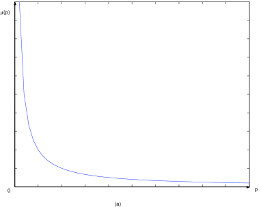
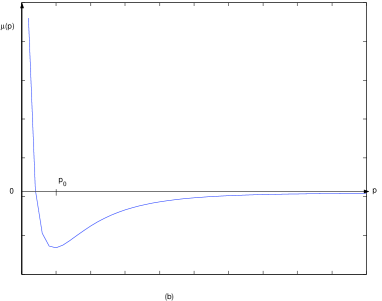
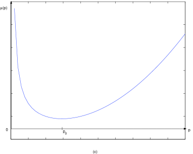
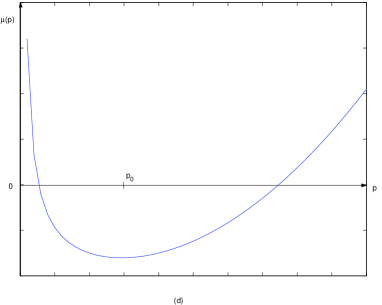
Figure 1. Possible profiles of the spectral function $\mu(p)$

We note that, for Maxwell models (A), (B), (C) of Boltzmann equation (Sections 2 and 3), only cases (a) and (b) of Fig.1 can be possible (actually this is the case (b)) since the condition (6.21) holds. Fig.1 gives a clear graphic representation of the domains of attraction of self-similar solutions (Lemma 6.4): it is sufficient to draw the line $\mu(p)=\mu_{*}={constant}$, and to consider a $p$ such that the graph of $\mu(p)$ lies below this line.

Therefore, the following corollary follows directly from the properties of the spectral function $\mu(p)$, as characterized by the behaviors in Fig.1, where we assume that $\mu(p_{0})=0$ for $p_{0}=\infty$, for the case shown on Fig.1 (a).

Corollary 4.

Any self-similar solution $u_{s}(x,t)=w(xe^{\mu_{*}t})$ with $\mu(p_{0})<\mu_{*}<\infty$ has a non-empty domain of attraction, where $p_{0}$ is the unique (minimum) critical point of the spectral function $\mu(p)$.

Proof.

We use Lemma 6.4 part ii) on any initial state $u_{0}=w+O(x^{p})$ with $p>0$ such that $\mu(p_{0})\leq\mu(p)<\mu_{*}$. In particular, Eqs. (6.15) and (6.16) show that the domain of attraction of $w(xe^{\mu_{*}t})$ contains any solution to the initial value problem (4.7) with the initial state as above. ∎

The inequalities of the kind $u_{1}-u_{2}=O(x^{p})$ for any $p>0$ such that $\mu(p)<\mu_{*}$, for any fixed $\mu_{*}\geq\mu(p_{0})$ play an important role for the self-similar stability. We can use specific properties of $\mu(p)$ in order to express such inequalities in a more convenient form.

Lemma 6.6.

For any given $\mu_{*}\in(\mu(p_{0}),\infty)$ and $u_{1,2}(x)$ such that $\|u_{1,2}\|<\infty$, the following two statements are equivalent:

• there exists $p>0$ such that

  $$u_{1}-u_{2}=O(x^{p})\ ,\qquad\text{with}\ \ \mu(p)<\mu_{*}\,.$$ (6.23)

• There exists $\varepsilon>0$ such that

  $$u_{1}-u_{2}=O(x^{{\mathrm{p}}(\mu_{*})+\varepsilon})\ ,\quad\ \text{ with}\ \ \mathrm{p}(\mu_{*})<p_{0}\ ,$$ (6.24)

  where $\mathrm{p}(\mu)$ is the inverse to $\mu(p)$ function, as defined in Corollary 2.

Proof.

Let property i) holds, then recall from Corollary 2 that $\mu(p)$ is monotone on the interval $0<p\leq p_{0}$, so its inverse function $\mathrm{p}(\mu)$ is defined uniquely.

It is clear, as it can be seen in from Fig.1, that the condition $\mu(p)<\mu_{*}$ are satisfied only for some $p>\mathrm{p}(\mu_{*})$, therefore inequality (6.24) with $\varepsilon=p-\mathrm{p}(\mu_{*})$ follows directly from (6.23).

Conversely, if ii) holds, first note that for any pair of uniformly bounded functions (note that $\|u_{1,2}\|<\infty$ by assumption) which satisfy inequality

$$|u_{1}(x)-u_{2}(x)|<C\,x^{q}\ ,\qquad C={const.}\ ,$$

for some $q>0$, then the same inequality holds with any $p$ such that $0<p<q$ and perhaps another constant. Therefore, if the condition (6.24) is satisfied, then one can always find a sufficiently small $0<\varepsilon_{1}\leq\varepsilon$ such that taking $p=\mathrm{p}(\mu_{*})+\varepsilon_{1}$ condition (6.23) is fulfilled. This completes the proof. ∎

Finally, to conclude this section, we show a general property of the initial value problem (4.7) for any non-linear $\Gamma$ operator satisfying conditions a) and b) given in Eqs. (6.1) and (6.2) respectively. This property gives the control to the point-wise difference of any two rescaled solutions to (4.7) in the unit sphere of B , whose initial states differ by $O(x^{p})$. It is formulated as follows.

Lemma 6.7.

Consider the problem (4.7), where $\Gamma$ satisfies the conditions (a) and (b). Let $u_{1,2}(x,t)$ are two solutions satisfying the initial conditions $u_{1,2}(x,0)=u_{0}^{1,2}(x)$ such that

$$\|u_{0}^{1,2}\|\leq 1\ ,\quad u_{0}^{1}-u_{0}^{2}=O(x^{p})\ ,\quad p>0\ .$$ (6.25)

then, for any real $\mu_{*}$,

$$\Delta_{\mu_{*}}(x,t)=u_{1}(xe^{-\mu_{*}t},t)-u_{2}(xe^{-\mu_{*}t},t)=O(x^{p})e^{-pt[\mu_{*}-\mu(p)]}$$ (6.26)

and therefore

$$\lim_{t\to\infty}\Delta_{\mu_{*}}(x,t)=0\ ,\qquad x\geq 0\ ,$$ (6.27)

for any $\mu_{*}>\mu(p)$.

Proof.

The proof is a repetition of arguments that led to Eq. (6.15)). In particular, we obtain from Eqs. (5.5), (6.8) the estimate

$$|u_{1}(x,t)-u_{2}(x,t)|=x^{p}\,e^{t[\lambda(p)-1]}\,\|\frac{u_{0}^{1}-u_{0}^{2}}{x^{p}}\|$$

and then change $x$ to $xe^{-\mu_{*}t}$. This leads to Eq. (6.26) in the notation (6.6) and this completes the proof. ∎

Remark.

There is an important point to understand here: Lemmas 6.2 and 6.4 hold for any operator $\Gamma$ that satisfies just the two properties (a) and (b) stated in (6.1) and (6.2). It says that, in some sense, a distance between any two solutions with initial conditions satisfying Eqs. (6.25) tends to zero as $t\to\infty$, i.e. non-expansive distance. Such terminology and corresponding distances were introduced in [18] for the elastic Maxwell-Boltzmann with finite initial energy, and for specific forms of Maxwell-Boltzmann models in [3, 22]. It should be pointed out, however, that this contraction property may not say much about large time asymptotics of $u(x,t)$, unless the corresponding self-similar solutions are known, for which the operator $\Gamma$ must be invariant under dilations (so it satisfies also property (c) as well, as stated in (6.3)). In such case one can use estimate (6.27) to deduce the pointwise convergence of characteristic functions $u(x,t)$ (Fourier or Laplace transforms of positive distributions, or equivalently, probability measures) in the form (6.15), (6.16) and the corresponding weak convergence in the space of probability measures [17]. We shall discuss these issues, in Sections 10  and 11 below, in more detail.

Therefore one must study the problem of existence of self-similar solutions, which is considered in the next Section.

7. Existence of self-similar solutions

The goal of this Section is to develop a criterion for existence, uniqueness and self-similar asymptotics to the problem Eq. (6.13) for any operator $\Gamma$ that satisfies conditions (a), (b) and (c) from Section 6, with the corresponding spectral function $\mu(p)$ defined in (6.6).

Theorem 7.1 below shows the criterion for existence and uniqueness of self-similar solutions for any operator $\Gamma$ that satisfies just conditions (a) and (b). Then Theorem 7.2 follows, showing a general criteria to self-similar asymptotics for the problem (4.7) for any operator $\Gamma$ that satisfying conditions (a), (b) and (c) and that $p_{0}>1$, for $\mu(p_{0})=\min_{P>0}\mu(p)$, in order to study the initial value problem with finite energy.

We consider Eq. (6.13) written in the form

$$\mu_{*}xw^{\prime}(x)+w(x)=g(x)\ ,\qquad g=\Gamma(w)\ ,\ \mu_{*}\in{\mathbb{R}}\ ,$$ (7.1)

and, assuming that $\|w\|<\infty$, transform this equation to the integral form. It is easy to verify that the resulting integral equation reads

$$w(x)=\int_{0}^{1}d\tau\,g(x\tau^{\mu_{*}})$$ (7.2)

We prove the following result.

Theorem 7.1.

Consider Eq. (7.1) with arbitrary $\mu_{*}\in{\mathbb{R}}$ and the operator $\Gamma$ satisfying the conditions (a) and (b) from Section 6. Assume that there exists a continuous function $w_{0}(x)$, $x\geq 0$, such that

• $\|w_{0}\|\leq 1$ and

• $$\int_{0}^{1}dt\,g_{0}(xt^{\mu_{*}})=w_{0}(x)+O(x^{p})\ ,\qquad\qquad g_{0}=\Gamma(w_{0})\ ,\hfill$$ (7.3)

  
  

  with some $p>0$ and $p\,\mu_{*}>-1$ satisfying the inequality

  $$\mu(p)=\frac{1}{p}\Big{[}\int_{0}^{\infty}da\,K(a)a^{p}-1\Big{]}<\mu_{*}\ .$$ (7.4)

• Then, there exists a classical solution $w(x)$ of Eq. (7.1).

• The solution is unique in the class of continuous functions satisfying conditions

  $$\|w\|\leq 1\ ,\qquad w(x)=w_{0}(x)+O(x^{p_{1}})\ ,$$ (7.5)

  with any $p_{1}$ such that $\mu(p_{1})<\mu_{*}$.

Proof.

The existence is proven by the following iteration procedure. We choose an initial approximation $w_{0}\in U$ such that $\|w_{0}\|\leq 1$ and consider the iteration scheme

$$w_{n+1}(x)=\int_{0}^{1}d\tau\,g_{n}(x\tau^{\mu_{*}})\ ,\qquad\qquad g_{n}=\Gamma(w_{n})\ ,\ n=0,1,\ldots\ .$$ (7.6)

Then, property (a) of $\Gamma$, $\|w_{n}\|\leq 1$ for all $n\geq 1$ and

$$|w_{n+1}(x)-w_{n}(x)|\leq\int_{0}^{1}d\tau\,|g_{n}(x\tau^{\mu_{*}})-g_{n-1}(x\tau^{\mu_{*}})|\ ,\qquad n\geq 1\,.$$

By using the inequality (6.2) (i.e. property (b) of $\Gamma$), we control the right hand side of the above inequality by, recalling the definition of the linear operator $L$ from (4.12)

$$|w_{n+1}(x)-w_{n}(x)|\leq\int_{0}^{1}d\tau\,L(|w_{n}-w_{n-1}|)(x\tau^{\mu_{*}})\\ =\int_{0}^{1}d\tau\,\int_{0}^{\infty}da\,K(a)|w_{n}-w_{n-1}|(ax\tau^{\mu_{*}})\ .$$ (7.7)

Next, by assumption ii), initially

$$w_{1}=w_{0}+O(x^{p})\ ,\qquad\mbox{with }\qquad p{\mu_{*}}>-1\ ,\ p>0\ ,$$ (7.8)

or, equivalently,

$$|w_{1}(x)-w_{0}(x)|\leq Cx^{p}\ ,\qquad x\geq 0\ ,\ C={const.}\ ,$$

then, recalling the definition for $\lambda(p)$ given in (6.5), we can control the right hand side of (7.7) by

$$x^{p}\,\int_{0}^{\infty}da\,K(a)a^{p}\int_{0}^{1}\tau^{p{\mu_{*}})}d\tau=x^{p}\frac{\lambda(p)}{1+p{\mu_{*}}}\ .$$

Therefore, we estimate the left hand side of (7.7) by

$$|w_{n+1}(x)-w_{n}(x)|\leq C\gamma^{n}(p,{\mu_{*}})x^{p}\ ,\qquad\gamma(p,{\mu_{*}})=\frac{\lambda(p)}{1+p{\mu_{*}}}\ .$$ (7.9)

Then, from condition ii) $\gamma(p,\mu_{*})>0$ since $p\mu_{*}>-1$. Also, from condition ii), (7.4), $\mu(p)=\frac{\lambda(p)-1}{p}<{\mu_{*}}$ implies $0<\gamma(p,\mu_{*})<1$.

Therefore, there exists a point-wise limit

$$w(x)=\lim_{n\to\infty}w_{n}(x)$$ (7.10)

satisfying the inequality

$$|w(x)-w_{0}(x)|\leq\sum_{n=0}^{\infty}|w_{n+1}-w_{n}(x)|\leq\frac{C}{1-\gamma(p,{\mu_{*}})}\ x^{p}\ .$$ (7.11)

Estimate (7.9) with $\gamma<1$ shows that the convergence $w_{n}(x)\to w(x)$ is uniform on any interval $0\leq x\leq R$, for any $R>0$. Therefore $w(x)$ is a continuous function, moreover $\|w\|\leq 1$ since $\|w_{n}\|\leq 1$ for all $n=0,1,\ldots$.

The next step is to prove that the limit function $w(x)$ from (7.10) satisfies Eqs. (7.1), or equivalently, (7.2). We note that

$$\begin{split}|g_{n+1}(x)-g_{n}(x)|&\leq\int_{0}^{\infty}da\,K(a)|w_{n+1}(ax)-w_{n}(ax)|\leq\\ &\leq C\,\lambda(p)\gamma^{n}(p,{\mu_{*}})x^{p}\ .\end{split}$$ (7.12)

Therefore $g_{n}(x)\to g(x)$, where $g(x)\in C({\mathbb{R}}_{+})$ and $\|g\|\leq 1$, since $\|g_{n}\|\leq 1$ for all $n$. In addition, from the continuity of the operator $\Gamma(u)$ for $\|u\|\leq 1$ follows that $g=\Gamma(w)$, and the transition to the limit in the right hand side of Eq. (7.2) is justified since $\|g_{n}\|\leq 1$. Hence, $w(x)$ satisfies Eq. (7.2).

When ${\mu_{*}}\neq 0$ one also needs to check that Eq. (7.1) is satisfied. We note that, for any continuous and bounded $w_{0}(x)$, all functions $w_{n}(x)$, $n\geq 1$, are differentiable for $x>0$ and their derivatives $w^{\prime}_{n}(x)$ satisfy the equations (see Eqs. (7.1), (7.6))

$${\mu_{*}}\,x\,w^{\prime}_{n}(x)=w_{n}(x)+g_{n-1}(x)\ ,\qquad n=1,2,\ldots\ .$$

Hence,

$${\mu_{*}}\,x\,(w^{\prime}_{n+1}-w^{\prime}_{n})=(w_{n}-w_{n+1})+(g_{n}-g_{n-1})\ ,$$

and, by using inequalities (7.9), (7.12), we obtain

$$|{\mu_{*}}|\,|w^{\prime}_{n+1}-w^{\prime}_{n}|\leq C\,\gamma^{p-1}(p,{\mu_{*}})\,(\gamma(p,{\mu_{*}})+\lambda(p))\,x^{p}\ ,\qquad n\geq 1\ .$$

Therefore the sequence of derivatives $\{w^{\prime}_{n}(x),\,n=1,\ldots\}$ converges uniformly on any interval $\varepsilon\leq x\leq R$. Hence, the limit function $w(x)$ from (7.10) is differentiable for $x>0$,

$$w^{\prime}(x)=O(x^{p-1})\ ,\qquad p>0\ ,$$ (7.13)

and the equality (7.1) is also satisfied for ${\mu_{*}}\neq 0$.

Finally we note that the condition of convergence $0<\gamma(p,{\mu_{*}})<1$, which is equivalent to the condition $\mu(p)<{\mu_{*}}$, (see Eq. (6.6)) that has already appeared in Lemma 6.4.

It remains to prove the statement concerning the uniqueness of the limit function $w(x)$ from (7.10). If there are two solutions $w^{{}_{1,2}}$ satisfying (7.1), then the integral equation (7.2) yields

$$|w^{{}_{1}}(x)-w^{{}_{2}}(x)|\leq\int_{0}^{1}d\tau\,|g^{{}_{1}}(x\tau^{\mu_{*}})-g^{{}_{2}}(x\tau^{\mu_{*}})|\ ,\qquad g^{{}_{1,2}}=\Gamma(w^{{}_{1,2}})\ .$$ (7.14)

Since $\|w^{{}_{1,2}}\|\leq 1$, we obtain

$$|w^{{}_{1}}(x)-w^{{}_{2}}(x)|\leq C\,x^{q}\ ,\qquad q=\min(p,p_{1})\ ,$$

where obviously $\mu(q)<{\mu_{*}}$. Then we again apply the inequality (6.2) to the integral in Eq. (7.2) and get the new estimate

$$|w^{{}_{1}}(x)-w^{{}_{2}}(x)|\leq C_{1}x^{q}\ ,\qquad C_{1}=\gamma(q,{\mu_{*}})C<C\ .$$

By repeating the same considerations as in the existence argument, it follows that

$$|w^{{}_{1}}(x)-w^{{}_{2}}(x)|\leq C\gamma^{n}(q,{\mu_{*}})x^{q}\ ,\qquad\text{ with }\ \ \gamma(q,{\mu_{*}})<1\ ,$$

for any integer $n\geq 0$. Therefore $w^{{}_{1}}(x)\equiv w^{{}_{2}}(x)$ and the proof is complete. ∎

Now we can combine Lemma 5.1 with Lemma 6.4 and prove the general statement related to the self-similar asymptotics for the problem (4.7).

Theorem 7.2.

Let $u(x,t)$ be a solution of the problem (4.7) with $\|u_{0}\|\leq 1$ and $\Gamma$ satisfying the conditions (a), (b), (c) from Section 6. Let $\mu(p)$ denote the spectral function (7.4) having its minimum (infimum) at $p=p_{0}$ (see Fig.1), the case $p_{0}=\infty$ is also included. We assume that there exists $p\in(0,p_{0})$ and $0<\varepsilon<p_{0}-p$ such that

$$\int_{0}^{1}d\tau\,g_{0}(x\tau^{\mu(p)})=u_{0}(x)+O(x^{p+\varepsilon})\ ,\qquad g_{0}=\Gamma(u_{0}),\quad\varepsilon>0\ .$$ (7.15)

Then

• there exists a unique solution $w(x)$ of the equation (7.1) with $\mu_{*}=\mu(p)$ such that

  $$\|w\|\leq 1\ ,\qquad w(x)=u_{0}(x)+O(x^{p+\varepsilon})\ ,$$ (7.16)

• $$\lim_{t\to\infty}u(x\,e^{-\mu(p)t},t)=w(x)\ ,\qquad x\geq 0\ ,$$ (7.17)

  where the convergence is uniform on any bounded interval in ${\mathbb{R}}_{+}$ and

  $$u(x\,e^{-\mu(p)t},t)-w(x)=O(x^{p+\varepsilon}e^{-\beta(p,\varepsilon)t})\,,$$ (7.18)

  with $\beta(p,\varepsilon)=(p+\varepsilon)(\,\mu(p)-\mu(p+\varepsilon)\,)>0$.

Proof.

If the condition (7.15) is satisfied, we can take $w_{0}=u_{0}(x)$ in the assumption ii) of Theorem 7.1. Indeed, the function $\mu(p)$ is monotone decreasing for $p\in(0,p_{0})$ and therefore invertible. We denote the inverse function by $p(\mu)$ and apply Lemma 6.6 to the condition ii) of Theorem 7.1. Thus we obtain for any $\mu_{*}\in(\mu(p_{0}),\infty)$ and $w_{0}=u_{0}$

$$\int_{0}^{1}d\tau\,g_{0}(x\tau^{\mu_{*}})=u_{0}+O(x^{p(\mu_{*})+\varepsilon})\ ,\qquad\varepsilon>0\ .$$ (7.19)

We note that the condition ii) cannot be fulfilled for any $\mu_{*}\leq\mu(p_{0})$ since the set $\mu(p)<\mu_{*}$ is empty in such case. Rewriting Eq. (7.19) in the equivalent form with $\mu_{*}=\mu(p)$ we obtain the condition (7.16). Then the statement i) follows from Theorem 7.1. Therefore we can apply Lemma 6.4 and obtain the limiting equality (7.17) and the estimate (7.18). This completes the proof. ∎

Thus we obtain a general criterion (7.16) of the self-similar asymptotics of $u(x,t)$ for a given initial condition $u_{0}(x)$. The criterion can be applied to the problem (4.7) with any operator $\Gamma$ satisfying conditions (a), (b), (c) from Section 6. The specific class (4.3) of operators $\Gamma$ is studied in Section 8. We shall see below that the condition (7.16) can be essentially simplified for such operators.

Remark.

One may expect a probabilistic connection between Theorems 7.1 and 7.2 on the relation of rates of convergence between rates of relaxation to these selfsimilar states and the convergence of the corresponding Wild convolution sums formulation for a non-conservative Maxwell model type. Such consideration may give place to results of a central limit theorem type for non classical statistical equilibrium stationary states. In the classical case of Maxwell Molecules models for energy conservation (that is for $\mu(1)=0$) with bounded initial energy, these connections has been fully established recently by [11, 12], where in this case the asymptotic states are Maxwellian equilibrium distributions.

8. Properties of self-similar solutions

The goal of this Section is to apply the general theory (in particular, Theorem 7.2) to the particular case of the multi-linear operators $\Gamma$ considered in Section 4, where their corresponding spectral function $\mu(p)$ satisfies (7.4), (4.13) and its behavior corresponds to Fig.1. We also show that $p_{0}>1$ is a necessary condition for self-similar asymptotics, for $p_{0}$ being the unique minimum of the spectral function, that is $\mu(p_{0})=\min_{p>0}\mu(p)$.

In addition, Theorem 8.3 establishes sufficient conditions for which self-similar solutions of problem (7.1) will lead to well defined self-similar solutions (distribution functions) of the original problem after taking the inverse Fourier transform.

We consider the integral equation (7.2) written as

$$w=\Gamma_{\mu}(w)=\int_{0}^{1}d\tau\,g(x\tau^{\mu})\ ,\qquad g=\Gamma(w)\ ,\ \mu\in{\mathbb{R}}\ .$$ (8.1)

First we establish two properties of $w(x)$ that are independent of the specific form (4.3) of $\Gamma$.

Lemma 8.1.

   

• If there exist a closed subset $U^{\prime}\subset U$ of the unit ball $U$ in $B$, as given in (4.15), such that $\Gamma_{\mu_{*}}(U^{\prime})\subset U^{\prime}$ for any $\mu_{*}\in{\mathbb{R}}$, and for some function $w_{0}\in U^{\prime}$ the conditions of Theorem 7.1 are satisfied, then $w\in U^{\prime}$, where $w$ is constructed by the iterative scheme as defined in (7.6).

• If the conditions of Theorem 7.1 for $\Gamma$ are satisfied and, in addition, $\Gamma(1)=1$,

then the solution $w_{*}=1$ of Eq. (8.1) is unique in the class of functions $w(x)$ satisfying the condition

$$w(x)=1+O(x^{p})\ ,\qquad\mu(p)<\mu_{*}\ .$$ (8.2)

Proof.

The first statement follows from the iteration scheme (7.6) with $w_{0}\in U^{\prime}$. Then, by assumption i, $w_{0}\in U^{\prime}$ for all integer $n\geq 1$, and $w_{n}\to w\in U^{\prime}$. The second statement follows from the obvious fact that $w_{*}=1$ satisfies Eq. (8.1) with any $\mu_{*}\in{\mathbb{R}}$ provided $\Gamma(1)=1$ and from the uniqueness of $w(x)$ stated in Theorem 7.1. This completes the proof. ∎

The statement ii can be interpreted as a necessary condition for existence of non-trivial ($w\neq\text{const.}$) solutions of Eq. (8.1):

if there exists a non-trivial solution $w(x)$ of Eq. (8.1) for any $\mu_{*}$, where $\Gamma(1)=1$, such that

$$\|w\|=1\ ,\qquad w=1+O(x^{p})\ ,\quad p>0\,,\ \ \ \ \ \text{{\it then}}\ \ \ \ \ \ \ \ \ \ \mu_{*}\leq\mu(p)\,.$$ (8.3)

We recall that $\mu(p)$ satisfies the inequality $\mu(p)\geq\mu(p_{0})=\min_{p>0}\mu(p)$ (see Fig.1).

Moreover, if $p\geq p_{0}$ (provided $p_{0}<\infty$) in Eqs. (8.3), then all solutions of Eq. (8.1) are trivial, for any $\mu_{*}>\mu(p_{0})$, since $\mu(p)$ is increasing in $(p_{0},\infty)$ .

On the other hand, possible solutions with $\mu\leq\mu(p_{0})$ (even if they exist) are irrelevant for the problem (4.7) since they have an empty domain of attraction (Lemma 6.4).

Therefore we always assume below that $\mu>\mu(p_{0})$ and, consequently, $p\in(0,p_{0})$ in Eq. (8.3).

Let us consider now the specific class (4.3)–(4.4) of operators $\Gamma$, with functions $u(x)$ satisfying the condition $u(0)=1$. That is, $u(0,t)=1$ for the solution $u(x,t)$ of the problem (4.7).

Since the operators (4.3) are invariant under dilation transformations (6.3) (property (c), Section 6), the problem (4.7) with the initial condition $u_{0}(x)$ satisfying

$$u(0)=1\ ,\quad\|u_{0}\|=1\ ;\qquad u_{0}(x)=1-\beta x^{p}+\cdots,\quad x\to 0\ ,$$ (8.4)

can be always reduced to the case $\beta=1$ by the transformation $x^{\prime}=x\beta^{1/p}$.

Moreover, the whole class of operators (4.3), with different kernels $A_{n}(a_{1},\ldots,a_{n})$, $n=1,2,\ldots$, is invariant under transformations $\tilde{x}=x^{p}$, $p>0$. The result of such transformation acting on $\Gamma$ is another operator $\widetilde{\Gamma}$ of the same class (4.3) with kernels $\tilde{A}_{n}(a_{1},\ldots,a_{n})$.

Therefore, we fix the initial condition (8.4) with $\beta=1$ and transform the function (8.4) and the Eq. (4.7) to new variables $\tilde{x}=x^{p}$. Then, we omit the tildes and reduce the problem (4.7), with initial condition (8.4) to the case $\beta=1$, $p=1$. We study this case, which correspond to finite energy, in detail and formulate afterward the results in terms of initial variables.

Next, our goal now is to apply the general theory (in particular, Theorem 7.2 and criterion (7.15)) to the particular case where the initial data $u_{0}(x)$ satisfies, for small $x$

$$\|u_{0}\|=1\ ,\quad u_{0}(x)=1-x+O(x^{1+\varepsilon})\ ,\quad x\to 0\ ,$$ (8.5)

with some $\varepsilon>0$.

We also assume that the spectral function $\mu(p)$ given by (7.4), (4.13), which corresponds to one of the four cases shown on Fig.1 with a unique minimum achieved at $p_{0}>1$.

We shall prove that any solution constructed by the iteration scheme of theorem (7.1) with ${\mu_{*}}=\mu(1)$, satisfying also the asymptotics from theorem (7.2) is controlled from below by $e^{-x}$ and that $\lim_{x\to\infty}w(x)=0$, as well as other properties with a significant meaning.

To this end, let us take a typical function $u_{0}=e^{-x}$ satisfying (8.5) and apply the criterion (7.15), from Theorem 7.2 or, equivalently, look for such $p>0$ for which (7.15) is satisfied. That is, find possible values of $p>0$ such that

$$\Gamma_{\mu(p)}(e^{-x})-e^{-x}=0(x^{p+\varepsilon})\,,$$ (8.6)

in the notation of Eq. (8.1).

It is important to observe that now the spectral function $\mu(p)$ is closely connected with the operator $\Gamma$ (see Eqs. (7.4) and (4.13)), since this was not assumed in the general theory of Sections 4–7. This connection leads to much more specific results, than, for example, the general Theorems 7.1, 7.2.

Then, in order to study the properties of self-similar solutions and its asymptotics to problem (7.1) for $p_{0}>1$, and consequently, for

$$\mu(p)\geq\mu(p_{0})>-\frac{1}{p_{0}}>-1\,,$$ (8.7)

we first investigate the structure of $\Gamma_{\mu}(e^{-x})$ for any $\mu>-1$. Its explicit formula reads

$$\Gamma_{\mu}(e^{-x})=\sum_{n=1}^{N}\alpha_{n}\int_{{\mathbb{R}}_{+}^{n}}da_{1}\ldots da_{n}A_{n}(a_{1},\ldots,a_{n})I_{\mu}\Big{[}x\sum_{k=1}^{n}a_{k}\Big{]}\ ,$$ (8.8)

where

$$I_{\mu}(y)=\int_{0}^{1}d\tau\,e^{-y\tau^{\mu}}\ ,\ \ \quad\mu\in{\mathbb{R}}\,,\ y>0\,,\qquad\qquad\sum_{n=1}^{N}\alpha_{n}=1\,.$$ (8.9)

Hence, in order to find some properties of $\Gamma_{\mu}(y)$, for any $\mu>-1$, we prove the following lemma.

Lemma 8.2.

If $\mu>-1$, $y\geq 0$, then $0<I_{\mu}(y)\leq 1$, and

$$I_{\mu}(y)=e^{-y}\left(1+\frac{\mu y}{1+\mu}\right)+\frac{\mu^{2}}{1+\mu}\,r_{\mu}(y)\ ,$$ (8.10)

where $0\leq r_{\mu}(y)\leq B(y,\mu)$ with

$$B(y,\mu)=\begin{cases}{y^{2}}{(2\mu+1)}^{-1}\ \qquad&\text{ if }\ \mu>-\frac{1}{2}\,,\\ 2y^{2}\left(-\ln y+y\right)\qquad&\text{ if }\ \mu=-\frac{1}{2}\,;\\ \frac{\Gamma(2-|\mu|^{-1})}{|\mu|}\ y^{\frac{1}{|\mu|}}\ &\text{ if }\ \mu\in\left(-1,-\frac{1}{2}\right)\ .\end{cases}$$ (8.11)

Proof.

We consider the integral $I_{\mu}(y)$, integrate twice by parts and obtain Eq. (8.10) with

$$r_{\mu}(y)=y^{2}\int_{0}^{1}\,e^{-y\tau^{\mu}}\tau^{2\mu}\,d\tau\ .$$

If $\mu>-1/2$ then the estimate (8.11) is obvious. Otherwise we transform $r_{y}(y)$ into the form

$$r_{\mu}(y)=\frac{1}{|\mu|}y^{\frac{1}{|\mu|}}\int_{y}^{\infty}e^{-\tau}\tau^{1-\frac{1}{|\mu|}}\,d\tau\ ,\qquad\mu\leq-\frac{1}{2}\ ,$$

so that the estimate (8.11) with $\mu\in(-1,-\frac{1}{2})$ is also clear.

Finally, in the case $\mu=-\frac{1}{2}$ we obtain

$$r_{-1/2}(y)=2y^{2}E(y)\ ,\qquad\text{with}\ \ E(y)=\int_{y}^{\infty}\frac{e^{-\tau}}{\tau}\,d\tau\ .$$

Hence, rewriting

$$\begin{split}E(y)&=\int_{1}^{\infty}\frac{e^{-\tau}}{\tau}\,d\tau+\int_{y}^{1}\,\frac{d\tau}{\tau}+\int_{y}^{1}(e^{-\tau}-1)\,\frac{d\tau}{\tau}\\ \vskip 6.0pt\cr&=-\ln y+\int_{0}^{y}(1-e^{-\tau})\,\frac{d\tau}{\tau}+C\ ,\end{split}$$

where $C$ is the well-known integral

$$C=\int_{1}^{\infty}\frac{e^{-\tau}}{\tau}\,d\tau+\int_{0}^{1}(e^{-\tau}-1)\,\frac{d\tau}{\tau}=\int_{0}^{\infty}e^{-\tau}\ln\tau\,d\tau=-\gamma\ ,$$

with $\gamma=\Gamma^{\prime}(1)\simeq 0.577$ is the Euler constant. Therefore, since $C<0$, and the function $(1-e^{-\tau})\tau^{-1}$ takes the value $1$ at the origin and is positive decreasing in $(0,y)$ for any $y>0$, then the term $E(y)$ is estimated by

$$E(y)\leq-\ln y+y\ .$$

Hence, we obtain the estimate (8.11) for $\mu=-1/2$ and the proof is completed. ∎

Hence, we can characterize now the possible values of $p>0$ for which criterion (7.15) holds, so Theorem 7.2 yields the self-similar asymptotics. We state and prove this characterization in the following corollary.

Corollary 5.

Whenever $p_{0}>1$ for $\mu(p_{0})=\min_{{}_{p>0}}\mu(p)$, the condition (8.6) is fulfilled if and only if $p\leq 1$ and, therefore, $\mu(p)\geq\mu(1)$ .

Proof.

From the previous Lemma we obtain

$$I_{\mu}(y)=1-\frac{y}{1+\mu}+O(y^{1+\varepsilon})\ ,\qquad\varepsilon>0\ ,\ y\to 0\ ,$$

provided $\mu>-1$. Therefore

$$\Gamma_{\mu}(e^{-x})-e^{-x}=\theta(\mu)x+O(x^{1+\varepsilon})\ ,$$

where

$$\theta(\mu)=1-\frac{1}{1+\mu}\sum_{n=1}^{N}\alpha_{n}\int_{{\mathbb{R}}_{+}^{n}}da_{1}\ldots da_{n}A_{n}(a_{1},\ldots,a_{n})\sum_{k=1}^{n}a_{k}\ .$$

We recall that kernels $A_{n}(a_{1},\ldots,a_{n})$, $n=1,\ldots,N$, are assumed to be symmetric functions of their arguments. Then

$$\theta(\mu)=1-\frac{1}{1+\mu}\lambda(1)\ ,\qquad\lambda(p)=\int_{0}^{\infty}da\,K(a)a^{p}\ ,$$ (8.12)

where $K(a)$ is given in Eqs. (4.13). Recalling the definition of $\mu(p)$ in (6.6), we obtain

$$\Gamma_{\mu(p)}(e^{-x})-e^{-x}=\theta[\mu(p)]x+O(x^{1+\varepsilon})\ ,$$ (8.13)

where

$$\theta[\mu(p)]=\frac{\mu(p)-\mu(1)}{1+\mu(p)}\ ,\qquad 0<p<p_{0}\ .$$ (8.14)

It follows from Eqs. (8.13), (8.14) that the condition (8.6) is fulfilled if and only if $p\leq 1$. On the other hand, it was assumed above that $p_{0}>1$, therefore $\mu(p)\geq\mu(1)$ for such values of $p$. Thus, Corollary 5 is proved.

∎

In addition, by Lemma 8.1 [ii], if ${\mu_{*}}>\mu(1)$ then the iteration scheme

$$w_{n+1}=\Gamma_{{\mu_{*}}}(w_{n})\ ,\qquad w_{0}=e^{-x}\ ,\ n=0,1,\ldots,$$ (8.15)

converges to the trivial solution $w=1$. Hence, the only nontrivial case corresponds to ${\mu_{*}}=\mu(1)$ in Eqs. (8.15).

Hence, according to Theorem 7.1, $w_{n}(x)\to w(x)$, where $w(x)$ is continuously differentiable function on $[0,\infty)$.

On the other hand,

$$w(x)=w_{0}(x)+O(x^{1+\varepsilon})$$ (8.16)

and therefore $w^{\prime}(0)=w^{\prime}_{0}(0)=-1$. Since this condition is not fulfilled for $w(x)=1$, we indeed obtain a non-trivial solution of Eq. (8.1) with ${\mu_{*}}=\mu(1)$.

Even though we would obtain the same result starting the iterations (8.15) from any initial function satisfying Eqs. (8.5), the specific function $w_{0}=e^{-x}$ has, however, some advantages since it gives some additional information about the properties of $w(x)$.

From now on we assume that ${\mu_{*}}=\mu(1)$ in Eqs. (8.15) and denote

$$w(x)=\lim_{n\to\infty}w_{n}(x)\ ,\qquad x\geq 0\ .$$ (8.17)

Then, by Theorem 7.1, $w\in C_{1}({\mathbb{R}}_{+})$ and satisfies the equation

$${\mu_{*}}\,x\,w^{\prime}(x)+w(x)=\Gamma(x)\ ,\qquad{\mu_{*}}=\mu(1)\ .$$ (8.18)

The differentiability of $w(x)$ was proved in Theorem 7.1 only for $\mu\neq 0$, but the proof can be easily extended to the case $\mu=0$ since $w_{0}=e^{-x}$ in Eqs. (8.15) has a bounded and continuous derivative.

From (8.15) and (8.16) it is clear that the limit function $w$ satisfies

$$0\leq w(x)\leq 1\ ,\qquad w(0)=1\ ,\ w^{\prime}(0)=-1\ ;$$ (8.19)

and, by considering a sequence of derivatives in Eqs. (8.15), it is easy to see that

$$w^{\prime}(x)\leq 0\ ,\qquad|w^{\prime}(x)|\leq 1\ .$$ (8.20)

Then, estimates from Theorem 7.1 and Lemma 8.2 yield that

$$w(x)=e^{-x}+O(x^{\pi({\mu_{*}})})\ ,$$ (8.21)

where

$$\pi({\mu_{*}})=\begin{cases}2\qquad\ \ &\text{ for }\ {\mu_{*}}>-\frac{1}{2}\ ,\\ 2-\varepsilon\text{ with any }\varepsilon>0\ &\text{ for }\ {\mu_{*}}=-\frac{1}{2}\ ,\\ \frac{1}{|{\mu_{*}}|}\ \ \ &\text{ for }\ -1<{\mu_{*}}<-\frac{1}{2}\ .\end{cases}$$ (8.22)

Hence, we collect all essential properties of $w(x)$ in the following statement.

Theorem 8.3.

The limiting function $w(x)$ constructed in (8.15) satisfies Eq. (8.1) with $\mu=\mu(1)$ and Eqs. (8.18), where $\Gamma$ is given in Eqs. (4.3), $\mu(p)$ is defined in Eqs. (7.4), (4.13). The conditions (8.19), (8.20), (8.21) are fulfilled for $w(x)$. Moreover

$$1\geq w(x)\geq e^{-x}\ ,\qquad\lim_{x\to\infty}w(x)=0\ ,$$ (8.23)

and there exists a generalized non-negative function $R(\tau)$, $\tau\geq 0$, such that

$$w(x)=\int_{0}^{\infty}d\tau\,R(\tau)e^{-\tau x}\ ,\qquad\int_{0}^{\infty}d\tau\,R(\tau)=\int_{0}^{\infty}d\tau\,R(\tau)\tau=1\ .$$ (8.24)

Proof.

It remains to prove (8.23) and (8.24). In fact condition (8.23) means that $e^{-x}$ is a barrier function to the solutions of problem (8.1) with $\mu=\mu(1)$.

First we note that Eq. (8.1) is obtained as the integral form of Eq. (7.1). Then, the identity

$$\mu\,x\,v^{\prime}(x)+v(x)=\Gamma(v)+\Delta(x)\,,$$

where

$$\Delta(x)=\mu\,x\,v^{\prime}(x)+v(x)-\Gamma(v)\,,$$ (8.25)

is fulfilled for any function $v(x)$, and the integral form of this identity reads

$$v(x)=\Gamma_{\mu}(v)+\int_{0}^{1}\Delta(x\tau^{\mu})\,d\tau\ .$$

Hence, if $\Delta(x)\leq 0$ then $v\leq\Gamma_{\mu}(v)$ and vice-versa.

We intend to prove that $\Delta(x)\leq 0$ for $v=e^{-x}$. If so, then $w_{n+1}(x)\geq w_{n}(x)$ at any $x\geq 0$ in the sequence (8.15) generated by the corresponding iteration scheme with $w_{0}=e^{-x}$, and obviously $w(x)\geq e^{-x}$.

Indeed, by substituting $v=e^{-x}$ in Eqs. (8.25) we obtain, for $\mu=\mu(1)$,

$$\Delta(x)=\sum_{n=1}^{\infty}\alpha_{n}\Delta_{n}(x)\ ,$$

where using (8.9),

$$\Delta_{n}(x)=\int_{{\mathbb{R}}_{+}^{n}}da_{1},\ldots,da_{n}A_{n}(a_{1},\ldots,a_{n})P\bigg{(}x,\sum_{k=1}^{n}a_{k}\bigg{)}\ ,\text{\ \ \ with}$$

$$P(x,s)=e^{-x}[1-(s-1)x]-e^{-sx}\leq 0\ .$$

We note that $P(x,s)\leq 0$ for any real $s$ and $x$, since $e^{y}\leq 1+y$ for any real $y$. Then $\Delta_{n}(x)\leq 0$, and so also $\Delta(x)\leq 0$. Hence, the inequality in (8.23) is proved.

In order to prove the limiting identity (8.23) we denote

$$w_{\infty}=\lim_{x\to\infty}w(x)\ .$$

Such limit exists since $w(x)$ is a monotone function. From theorem 8.3, the nice properties of $w(x)$ allow to take the limit in both sides of Eq. (8.1). Then

$$w_{\infty}=\sum_{n=1}^{N}\alpha_{n}w_{\infty}^{n}\ ,\qquad\sum_{n=1}^{N}\alpha_{n}=1\ ,\quad\alpha_{n}\geq 0\ ,$$

and therefore we obtain

$$\sum_{n=2}^{\infty}\alpha_{n}w_{\infty}(1-w_{\infty}^{n-1})=0\ .$$

This equation has just two non-negative roots: $w_{\infty}=0$ and $w_{\infty}=1$. The root $w_{\infty}=1$ is possible only if $w(x)=1$ for all real $x$. Since by (8.16) this is not the case, then $w_{\infty}=0$.

It remains to prove the integral representation (8.24). In order to do this we denote by $U^{\prime}$ the set of Laplace transforms of probability measures in ${\mathbb{R}}_{+}$, i.e., $u\in U^{\prime}$ if there exists a generalized function $F(\tau)\geq 0$ such that

$$u(x)=\int_{0}^{\infty}d\tau\,F(\tau)e^{-x{\tau}}\ ,\qquad\int_{0}^{\infty}d\tau\,F(\tau)=1\ .$$

Then $e^{-x}\in U^{\prime}$ (with $F=\delta(\tau-1)$) and it is easy to check that $\Gamma_{\mu}(U^{\prime})\subset U^{\prime}$ for any real $\mu$. On the other hand, the set $U^{\prime}$ is closed with respect to uniform convergence in ${\mathbb{R}}_{+}$ (see, for example, [17]). Thus, according to Lemma 8.1 [i], $w\in U^{\prime}$. On the other hand, it is already known from (8.19) that $w^{\prime}(0)=-1$. Hence, the corresponding function $R(\tau)$ has a unit first moment [17]. This completes the proof of Theorem 8.3. ∎

The integral representation (8.24) is important for the properties of the corresponding distribution functions satisfying Boltzmann-type equations. Now it is easy to return to initial variables with $u_{0}$ given in Eq. (8.4) and to describe the complete picture of the self-similar relaxation for the problem (4.7).

9. Main results for Fourier transformed Maxwell models
with multiple interactions

We consider the Cauchy problem (4.7) with a fixed operator $\Gamma$ (4.3) and study the time evolution of $u_{0}(x)$ satisfying the conditions

$$\|u_{0}\|=1\ ;\quad u_{0}=1-x^{p}+O(x^{p+\varepsilon})\ ,\ x\to 0\ ,$$ (9.1)

with some positive $p$ and $\varepsilon$. Then there exists a unique classical solution $u(x,t)$ of the problem (4.7), (9.1) such that, for all $t\geq 0$,

$$\|u(\cdot,t)\|=1\ ;\qquad u(x,t)=1+O(x^{p})\ ,\ x\to 0\ .$$ (9.2)

We explain below the simplest way to analyze this solution, in particular in the case of self-similar asymptotics.

Step 1. Consider the linearized operator $L$ given in Eqs. (4.12)–(4.13) and construct the spectral function $\mu(p)$ given in Eq. (7.4). The resulting $\mu(p)$ will be of one of four kinds described qualitatively on Fig.1.

Step 2. Find the value $p_{0}>0$ where the minimum (infimum) of $\mu(p)$ is achieved. Note that $p_{0}=\infty$ just for the case described on Fig.1 (a), otherwise $0<p_{0}<\infty$. Compare $p_{0}$ with the value $p$ from Eqs. (9.1).

If $p<p_{0}$ then the problem (4.7), (9.1) has a self-similar asymptotics (see below).

The above consideration shows that two different cases are possible:

• $p\geq p_{0}$ provided $p_{0}<\infty$;

• $0<p<p_{0}$, that is the spectral function $\mu(p)$ in monotone decreasing for all $0<p<p_{0}$.

In case (1) a behavior of $u(x,t)$ for large $t$ may depend strictly on initial conditions. The only general conclusion that can be drawn for the initial data (9.1) with $p\geq p_{0}$ is the following:

$$\lim_{t\to\infty}u(xe^{-\mu t},t)=1\ ,\qquad x\geq 0\ ,$$ (9.3)

for any $\mu>\mu(p_{0})$. This follows from Lemma 6.7 with $u^{(1)}=u$, $u^{(2)}=1$ and from the fact that any such function $u_{0}(x)$ satisfies the condition

$$u_{0}=1+O(x^{p_{0}})$$

Case (2) with $0<p<p_{0}$ in Eqs. (9.1) is more interesting. In this case (assume that $p\in(0,p_{0})$ is fixed) there exists a unique self-similar solution

$$u_{s}(x,t)=\psi(xe^{\mu(p)t})$$ (9.4)

satisfying Eqs. (8.1) at $t=0$. We again use Lemma 6.7 with $u_{1}=u$ and $u_{2}=u_{s}$ and obtain for the solution $u(x,t)$ of the problem (4.7), (9.1):

$$\lim_{t\to\infty}u(xe^{-\mu t},t)=\begin{cases}1&\text{if }\ \mu>\mu(p)\\ \psi(x)&\text{if }\ \mu=\mu(p)\\ 0&\text{if }\ \mu(p)>\mu>\mu(p+\delta)\ ,\end{cases}$$ (9.5)

with sufficiently small $\delta>0$. The third equality follows from the fact that

$$u_{0}(x)-\psi(x)=O(x^{p+\varepsilon})$$

and from the equality (see Eqs. (8.23))

$$\lim_{x\to\infty}\psi(x)=0\ .$$

We note that $\psi(x)=w(x^{p})$, where $w(x)$ has all properties described in Theorem 8.3. The equalities (9.5) explain the exact meaning of the approximate identity,

$$u(x,t)\approx\psi(xe^{\mu(p)t})\ ,\qquad t\to\infty\ ,\ xe^{\mu(p)t}=\text{const.}\ ,$$ (9.6)

that we call self-similar asymptotics. We collect the results in the following statement.

Proposition 9.1.

The solution $u(x,t)$ of the problem (4.7), (9.1), with $\Gamma$ given in Eqs. (4.3), satisfies either one of the following limiting identities:

• Eq. (9.3) if $p\geq p_{0}$ for the initial data (9.1)  ,

• Eqs. (9.5) provided $0<p<p_{0}$.

The convergence in Eqs. (9.3), (9.5) is uniform on any bounded interval $0\leq x\leq R$, and

$$u(xe^{\mu(p)t},t)-\psi(x)=O(x^{p+\varepsilon})e^{-\beta(p,\varepsilon)t}\,,\qquad\beta(p,\varepsilon)=(p+\varepsilon)\,(\mu(p)-\mu(p+\varepsilon)\,),$$

for $0<p<p_{0}$ and $0<\varepsilon<p_{0}-p$.

Proof.

It remains to prove the last statement. It follows in both cases from the estimate (6.26) for the remainder term in Lemma (6.7). This completes the proof. ∎

It is interesting that our considerations are the same for both positive and negative values of $\mu(p)$. There are, however, certain differences if we want to consider the “pure” large time asymptotics, i.e., the limits (9.3), (9.5) with $\mu=0$. Then we can conclude that

$$\begin{split}\text{\bf(1)}\quad&\lim_{t\to\infty}u(x,t)=1\ \ \ \ \ \ \ \ \text{if}\ \ p\geq p_{0}\text{ and }\mu(p_{0})<0\,,\ \text{ or }0<p<p_{0}\text{ and }\mu(p)<0\ ;\\ \text{\bf(2)}\quad&\lim_{t\to\infty}u(x,t)=\psi(x)\ \ \text{ if }\ \ 0<p<p_{0}\text{ and }\mu(p)=0\ .\end{split}$$

It seems probable that $u(x,t)\to 0$ for large $t$ in all other cases, but our results, obtained on the basis of Lemma 6.7, are not sufficient to prove this.

Remark.

We mention that the self-similar asymptotics becomes more transparent in logarithmic variables

$$y=\ln x\ ,\quad u(x,t)=\hat{u}(y,t)\ ,\quad\psi(x,t)=\hat{\psi}(y,t)$$

Then Eq. (9.6) reads

$$\hat{u}(y,t)\approx\hat{\psi}(y+\mu(p)t)\ ,\qquad t\to\infty\ ,\quad y+\mu(p)t=\text{const. },$$ (9.7)

i.e., the self-similar solutions are simply nonlinear waves (note that $\psi(-\infty)=1$, $\psi(+\infty)=0$) propagating with constant velocities $c_{p}=-\mu(p)$ to the right if $c_{p}>0$ or to the left if $c_{p}<0$. If $c_{p}>0$ then the value $u(-\infty,t)=1$ is transported to any given point $y\in{\mathbb{R}}$ when $t\to\infty$. If $c_{p}<0$ then the profile of the wave looks more natural for the functions $\tilde{u}=1-\hat{u}$, $\tilde{\psi}=1-\psi$.

Thus, Eq. (4.7) can be considered in some sense as the equation for nonlinear waves. The self-similar asymptotics (9.7) means a formation of the traveling wave with a universal profile for a broad class of initial conditions. This is a purely non-linear phenomenon, it is easy to see that such asymptotics cannot occur in the particular case ($N=1$ in Eqs. (4.3)) of the linear operator $\Gamma$.

10. Distribution functions, moments and power-like tails

We have described above the general picture of the behavior of the solutions $u(x,t)$ to the problem (4.7), (9.1). On the other hand, Eq. (4.7) (in particular, its special case (3.2)) was obtained as the Fourier transform of the kinetic equation. Therefore we need to study in more detail the corresponding distribution functions.

We assume in this section that $u_{0}(x)$ in the problem (4.7) is an isotropic characteristic function of a probability measure in ${\mathbb{R}}^{d}$, i.e.,

$$u_{0}(x)={\mathcal{F}}[f_{0}]=\int_{{\mathbb{R}}^{d}}dv\,f_{0}(|v|)e^{-ik\cdot v}\ ,\qquad k\in{\mathbb{R}}^{d}\ ,\ x=|k|^{2}\ ,$$ (10.1)

where $f_{0}$ is a generalized positive function normalized such that $u_{0}(0)=1$ (distribution function). Let $U$ be a closed unit ball in the $B=C({\mathbb{R}}_{+})$ as defined in (4.9). Then, as was already mentioned at the end of Section 5, the set $U^{\prime}\subset U$ of isotropic characteristic functions is a closed convex subset of $U$. Moreover, $\Gamma(U^{\prime})\subset U^{\prime}$ if $\Gamma$ is defined in Eqs. (4.3). Hence, we can apply Lemma 5.3 and conclude that there exists a distribution function $f(v,t)$, $v\in{\mathbb{R}}^{d}$, satisfying Eq. (2.1), such that

$$u(x,t)={\mathcal{F}}[f(\cdot,t)]\ ,\qquad x=|k|^{2}\ ,$$ (10.2)

for any $t\geq 0$.

A similar conclusion can be obtain if we assume the Laplace (instead of Fourier) transform in Eqs. (10.1). Then there exists a distribution function $f(v,t)$, $v>0$, such that

$$u(x,t)={\mathcal{L}}[f(\cdot,t)]=\int_{0}^{\infty}dv\,f(v,t)e^{-xv}\ ,\qquad u(0,t)=1\ ,\ \ x\geq 0\,,\ \ t\geq 0\ ,$$ (10.3)

where $u(x,t)$ is the solution of the problem (4.7) constructed in Theorem 5.2 and Lemma 5.3.

We remind the reader that the point-wise convergence $u_{n}(x)\to u(x)$, $x\geq 0$, where $\{u_{n},\,n=1,2,\ldots\}$ and $u$ are characteristic functions (or Laplace transforms) is sufficient for the weak convergence of the corresponding probability measures [17]. Hence, all results of pointwise convergence related to self-similar asymptotics can be easily re-formulated in corresponding terms for the related distribution functions (or, equivalently, probability measures).

The approximate equation (9.6) in terms of distribution functions (10.2) reads

$$f(|v|,t)\simeq e^{-\frac{d}{2}\mu(p)\,t}F_{p}(|v|e^{-\frac{1}{2}\mu(p)\,t})\ ,\quad t\to\infty\ ,\ |v|e^{-\frac{1}{2}\mu(p)\,t}=\text{const.}\ ,$$ (10.4)

where $F_{p}(|v|)$ is a distribution function such that for $x=|k|^{2}$

$$\psi_{p}(x)={\mathcal{F}}[F_{p}]\ \ ,$$ (10.5)

with $\psi_{p}$ given in Eq. (9.4) (the notation $\psi_{p}$ is used in order to stress that $\psi$ defined in (9.4), depends on $p$). The factor $1/2$ in Eqs. (10.4) is due to the notation $x=|k|^{2}$. Similarly, for the Laplace transform (10.3), we obtain

$$f(v,t)\simeq e^{-\mu(p)t}\Phi_{p}(ve^{-\mu(p)t})\ ,\qquad t\to\infty\ ,\ ve^{-\mu(p)t}=\text{const.}\ ,$$ (10.6)

where

$$\psi_{p}(x)={\mathcal{L}}[\Phi_{p}]\ .$$ (10.7)

In the space of distributions, the approximate relation $\simeq$ is weak in the sense of distributions, i.e. the classical approximation concept of real valued expression obtained after integrating by test functions.

The positivity and some other properties of $F_{p}(|v|)$ follow from the fact that $\psi_{p}(x)=w_{p}(x^{p})$, where $w_{p}(x)$ satisfies Theorem 8.3. Hence

$$\psi_{p}(x)=\int_{0}^{\infty}d\tau\,R_{p}(\tau)e^{-\tau x^{p}}\ ,\qquad\int_{0}^{\infty}d\tau\,R_{p}(\tau)=\int_{0}^{\infty}d\tau\,R_{p}(\tau)\tau=1\ ,$$ (10.8)

where $R_{p}(\tau)$, $\tau\geq 0$, is a non-negative generalized function (of course, both $\psi_{p}$ and $R_{p}$ depend on $p$).

We stress here that if $u_{0}(x)$ is a characteristic function given in Eq. (10.1), and condition (9.1) is fulfilled, then $p\leq 1$ in Eqs. (9.1). In addition, the case $p>1$ is impossible for the non-negative initial distribution $f_{0}$ in Eqs. (10.1) since

$$u^{\prime}(0)=-C_{d}\int_{{\mathbb{R}}^{d}}dv\,f_{0}(|v|)|v|^{2}\ ,$$ (10.9)

where $C_{d}>0$ is a constant factor that depends only on the space dimension for the problem.

Hence, the self-similar asymptotics (10.4) for any initial data $f_{0}\geq 0$ occurs if $p_{0}>1$ (see Step 2 at the beginning of Section 9). Otherwise it occurs for $p\in(0,p_{0})\subset(0,1)$. Therefore, for any spectral function $\mu(p)$ (Fig.1), the approximate relation (10.4) holds for sufficiently small $0<p\leq 1$. It follows from Eq. (10.9) that

$$m_{2}=\int_{{\mathbb{R}}^{d}}dv\,f_{0}(|v|)|v|^{2}<\infty\ \text{ if }\ p=1$$

and $m_{2}=\infty$ if $p<1$.

Similar conclusions can be made for the Laplace transforms (10.3) since in that case

$$u^{\prime}(0,t)=-\int_{0}^{\infty}dv\,f(v,t)v\ ,$$

therefore the first moment of $f$ plays the same role as the second moment in case of Fourier transforms.

The positivity of $F(|v|)$ in Eqs. (10.5) and (10.7) follows from the integral representation (10.8) with $p\leq 1$. It is well-known that

$${\mathcal{F}}^{-1}(e^{-|k|^{2p}})>0\ ,\qquad{\mathcal{L}}^{-1}(e^{-x^{2p}})>0$$

for any $0<p\leq 1$ (the so-called infinitely divisible distributions [17]). Thus, Eqs. (10.8) explains the connection of the self-similar solutions of generalized Maxwell models with infinitely divisible distributions. We can use standard formulas for the inverse Fourier (Laplace) transforms and denote ($d=1,2,\ldots$ is fixed)

$$\begin{split}M_{p}(|v|)&=\frac{1}{(2\pi)^{d}}\int_{{\mathbb{R}}^{d}}dke^{-|k|^{2p}+ik\cdot v}\ ,\\ \vskip 6.0pt\cr N_{p}(v)&=\frac{1}{2\pi i}\int_{a-i\infty}^{a+i\infty}dx\,e^{-x^{p}+xv}\ ,\qquad 0<p\leq 1\ .\end{split}$$ (10.10)

Then the self-similar solutions $F_{p}$ and $\Phi_{p}$ (distribution functions) given in the right hand sides of Eqs. (10.6) and (10.8) respectively, satisfy

$$\begin{split}F_{p}(|v|)&=\int_{0}^{\infty}d\tau\,R_{p}(\tau)\tau^{-\frac{d}{2p}}M_{p}(|v|\tau^{-\frac{1}{2p}})\ ,\\ \vskip 6.0pt\cr\Phi_{p}(v)&=\int_{0}^{\infty}d\tau\,R_{p}(\tau)\tau^{-\frac{1}{p}}N_{p}(v\tau^{-\frac{1}{p}})\ ,\qquad v\geq 0\ ,\ 0<p\leq 1\ .\end{split}$$ (10.11)

That is, they admit an integral representation through infinitely divisible distributions. Note that $M_{1}(|v|)$ is the standard Maxwellian in ${\mathbb{R}}^{d}$. The functions $N_{p}(v)$ (10.10) are studied in detail in the literature [17, 19].

Thus, for given $0<p\leq 1$, the kernel $R_{p}(\tau)$, $\tau\geq 0$, is the only unknown function that is needed to describe the distribution functions $F_{p}(|v|)$ and $\Phi_{p}(v)$. Therefore we study $R_{p}(\tau)$ in more detail.

It was already noted in Section 8 that the general problem (8.1), (8.3), with given $0<p<p_{0}$, can be reduced to the case $p=1$ by the transformation of variables $\tilde{x}=x^{p}$. We assume therefore that such transformation is already made and consider the case $p=1$. Then the equation for $R(\tau)=R_{1}(\tau)$ can be obtained (see Eqs. (8.24)) by applying the inverse Laplace transform to Eq. (8.18). Then we obtain, with ${\mu_{*}}=\mu(1)$,

$$-\mu(1)\frac{\partial}{\partial\tau}\tau R(\tau)+R(\tau)=Z(R)={\mathcal{L}}^{-1}[\Gamma(w)]\ ,$$ (10.12)

where (see Eqs. (4.3))

$$\begin{split}&Z(R)=\sum_{n=1}^{N}\alpha_{n}Z_{n}(R)\ ,\qquad\sum_{n=1}^{N}\alpha_{n}=1\ ,\ \alpha_{n}\geq 0\ ,\\ \vskip 6.0pt\cr&Z_{n}(R)=\int_{{\mathbb{R}}_{+}^{n}}da_{1},\ldots,da_{n}\frac{A_{n}(a_{1},\ldots,a_{n})}{a_{1}a_{2}\ldots a_{n}}\prod_{k=1}^{n}{\!\vphantom{\sum}}^{*}R\Big{(}\frac{\tau}{a_{k}}\Big{)}\ ,\\ \vskip 6.0pt\cr&\prod_{k=1}^{n}{\!\vphantom{\sum}}^{*}R_{k}(\tau)=R_{1}*R_{2}*\ldots*R_{n}\ ,\qquad R_{1}*R_{2}=\int_{0}^{\tau}d\tau^{\prime}\,R_{1}(\tau^{\prime})R_{2}(\tau-\tau^{\prime})\ .\end{split}$$

Let us denote

$$m_{s}=\int_{0}^{\infty}d\tau\,R(\tau)\tau^{s}\ ,\qquad s>0\ ,$$ (10.13)

then multiply Eq. (10.12) by $\tau^{s}$ and obtain after integration the following equality

$$\begin{split}&(\mu(1)s+1)m_{s}=\\ &=\sum_{n=1}^{N}\alpha_{n}\int_{{\mathbb{R}}_{+}^{n}}\mkern-18.0muda_{1}\ldots da_{n}A_{n}(a_{1},\ldots,a_{n})\int_{{\mathbb{R}}_{+}^{n}}\mkern-18.0mud\tau_{1}\ldots,d\tau_{n}\bigg{(}\sum_{k=1}^{n}a_{k}\tau_{k}\bigg{)}^{s}\prod_{j=1}^{n}R(\tau_{j})\ .\end{split}$$ (10.14)

Next, we recall the notations (4.13), (6.5), (6.6)

$$\begin{split}\lambda(p)&=\int_{0}^{\infty}da\,K(a)a^{p}=\sum_{n=1}^{N}\alpha_{n}\int_{{\mathbb{R}}_{+}^{n}}da_{1}\ldots da_{n}A_{n}(a_{1},\ldots,a_{n})\bigg{(}\sum_{k=1}^{n}a_{k}^{p}\bigg{)}\ ,\end{split}$$

and

$$\begin{split}\mu(p)&=\frac{\lambda(p)-1}{p}\ ,\end{split}$$

then Eq. (10.12) equation can be written in the form

$$(s\mu(1)+\lambda(s)-1)m_{s}=\sum_{n=2}^{N}\alpha_{n}I_{n}(s)\ ,$$ (10.15)

where

$$\begin{split}&I_{n}(s)=\int_{{\mathbb{R}}_{+}^{n}}\mkern-18.0muda_{1}\ldots da_{n}A(a_{1},\ldots,a_{n})\int_{{\mathbb{R}}_{+}^{n}}\mkern-18.0mud\tau_{1}\ldots,d\tau_{n}\;g_{n}^{(s)}(a_{1}\tau_{1},\ldots,a_{n}\tau_{n})\prod_{j=1}^{n}R(\tau_{j})\\ \vskip 6.0pt\cr&g_{n}^{(s)}(y_{1},\ldots,y_{n})=\bigg{(}\sum_{k=1}^{n}y_{k}\bigg{)}^{s}-\sum_{k=1}^{n}y_{k}^{s}\ ,\qquad n=1,2,\ldots\ .\end{split}$$ (10.16)

We note that $g_{1}^{(s)}=0$ for any $s\geq 0$ and that $m_{0}=m_{1}=1$ (see Eqs. (10.8)). Our aim is to study the moments $m_{s}$ (10.13), $s>1$, on the basis of Eq. (10.15). The approach is related to the one used in [22] for a simplified version of Eq. (10.15) with $N=2$. The main results are formulated below in terms of the spectral function $\mu(p)$ (see Fig.1) under the assumption that $p_{0}>1$.

Proposition 10.1.

   

• If the equation $\mu(s)=\mu(1)$ has the only solution $s=1$, then $m_{s}<\infty$ for any $s>0$.

• If this equation has two solutions $s=1$ and $s=s_{*}>1$, then $m_{s}<\infty$ for $s<s_{*}$ and $m_{s}=\infty$ for $s>s_{*}$.

• $m_{s_{*}}<\infty$ only if $I_{n}(s_{*})=0$ in Eq. (10.15) for all $n=2,\ldots,N$.

Proof.

The proof is based on the inequality

$$0\leq\sum_{n=2}^{N}\alpha_{n}I_{n}(s)\leq C_{N}(s)m_{1}m_{s-1}$$ (10.17)

with $s>1$ and some positive constant $C_{N}(s)$. Then we obtain

$$m_{s}\leq\frac{C_{N}(s)}{s[\mu(1)-\mu(s)]}\ m_{s-1}\ ,\qquad m_{0}=m_{1}=1\ .$$

In the case [i] $\mu(1)>\mu(s)$ (see Fig.1) for all $s$. The same is true in the case [ii] for $s<s_{*}$. It is clear from Eq. (10.13) that $m_{s}>0$ since $R(\tau)\geq 0$ and $m_{1}=1$. This means that the inequality (10.17) cannot be satisfied for $s>s_{*}$, therefore moments of orders $s>s_{*}$ cannot exist. The statement [iii] follows directly from Eq. (10.15). ∎

Hence, it remains to prove the inequality (10.17). The proof is based on the following elementary inequality.

Lemma 10.2.

In the notation of Eqs. (10.16),

$$0\leq g_{n}^{(s)}(y_{1},\ldots,y_{n})\leq 2^{s-1}s\bigg{\{}\psi(y_{1},y_{2})+\sum_{k=2}^{n-1}\gamma_{k}\psi(y_{k+1},Y_{k})\bigg{\}}\ ,\qquad s>1\ ,$$ (10.18)

where the second term (sum) is absent for $n=2$ and

$$\begin{split}&\psi(y_{1},y_{2})=y_{1}^{s-1}y_{2}+y_{2}^{s-1}y_{1}\ ,\qquad Y_{k}=\max(y_{1},\ldots,y_{k})\ ,\\ \vskip 6.0pt\cr&\gamma_{k}=\max(k,k^{s-1})\ ,\qquad k=1,\ldots,n\ ;\ n=2,3,\ldots\end{split}$$

Proof.

If $n=2$, we assume without loss of generality that $y_{1}\leq y_{2}$ and reduce the problem (upper estimate) to the inequality

$$\Delta(x)=(1+s)^{s}-1-x^{s}-2^{s-1}s(x+x^{s-1})\leq 0\ ,\qquad x=\frac{y_{1}}{y_{2}}\leq 1\ .$$

Its proof is obvious since, $\Delta(0)=0$, $\Delta^{\prime}(x)\leq 0$. The lower estimate in Eqs. (10.18) is similarly reduced for $n=2$ to the inequality

$$g(\theta)=1-\theta^{s}-(1-\theta)^{s}\geq 0\ ,\qquad\theta=\frac{x}{x+y}\leq 1\ .$$

Then, its proof follows from the fact that $g(0)=g(1)=0$, $g^{\prime\prime}(\theta)\leq 0$.

We proceed by induction. It is easy to see that

$$g_{n+1}^{(s)}(y_{1},\ldots,y_{n+1})=g_{n}^{(s)}(y_{1},\ldots,y_{n})+g_{2}^{(s)}\bigg{(}y_{n+1},\sum_{k=1}^{n}y_{k}\bigg{)}\ ,\qquad n=3,\ldots\ .$$

Then the lower estimate (10.18) becomes obvious for any $n\geq 2$. By applying the upper estimate (10.18) for $g_{2}(s)$ we obtain

$$g_{n+1}^{(s)}(y_{1},\ldots,y_{n+1})\leq g_{n}^{(s)}+2^{s}s\psi\bigg{(}y_{n+1},\sum_{k=1}^{n}y_{k}\bigg{)}$$

and note that $\psi(x,y)$ is an increasing function of $y$. Obviously

$$\sum_{k=1}^{n}y_{k}\leq nY_{n}\ ,\qquad Y_{n}=\max(y_{1},\ldots,y_{n})\ ,$$

and therefore

$$g_{n+1}^{(s)}(y_{1},\ldots,y_{n+1})\leq g_{n}^{(s)}(y_{1},\ldots,y_{n})+2^{s}s\gamma_{n}\psi(y_{n+1},Y_{n})\ .$$

This is precisely what is needed to get the upper estimate (10.18) by induction. This completes the proof of the lemma.∎

In order to complete the proof of the inequality (10.17) we substitute the estimates (10.18) into the right hand side of Eq. (10.15). Then the lower estimate (10.17) becomes obvious. The upper estimate (10.17) also becomes obvious if we note that

$$\max(a_{1}\tau_{1},\ldots,a_{k}\tau_{k})\leq\bar{a}_{n}\max(\tau_{1},\ldots,\tau_{k})\ ,\quad\bar{a}_{n}=\max(a_{1},\ldots,a_{n})\ ,\ k=1,\ldots,n\ ;$$

and

$$\begin{split}&\int_{{\mathbb{R}}_{+}^{k}}d\tau_{1}\ldots d\tau_{k}\bigg{(}\prod_{j=1}^{k}R(\tau_{j})\bigg{)}[\max(\tau_{1},\ldots,\tau_{k})]^{s}a=\\ \vskip 6.0pt\cr&\qquad=n!\int_{0\leq\tau_{1}\leq\cdots\leq\tau_{k}<\infty}\mkern-64.0mud\tau_{1}\ldots d\tau_{k}\bigg{(}\prod_{j=1}^{k}R(\tau_{j})\bigg{)}\tau_{k}^{s}\leq n!m_{s}\ ,\qquad s>0\ .\end{split}$$

Then it is trivial to show that the upper estimate (10.17) holds. This completes the proof of Proposition 10.1 ∎

Now we can draw some conclusions concerning the moments of the distribution functions (10.11). We denote

$$\begin{split}m_{s}(\Phi_{p})&=\int_{0}^{\infty}dv\,\Phi_{p}(v)v^{s}\ ,\qquad m_{s}(R_{p})=\int_{0}^{\infty}d\tau\,R_{p}(\tau)\tau^{s}\ ,\\ \vskip 6.0pt\cr m_{2s}(F_{p})&=\int_{{\mathbb{R}}^{d}}dv\,F_{p}(|v|)|v|^{2s}\ ,\qquad s>0\ ,\ 0<p\leq 1\ ,\end{split}$$

and use similar notations for $N_{p}(v)$ and $M_{p}(|v|)$ in Eqs. (10.11). Then, by formal integration of Eqs. (10.11), we obtain

$$\begin{split}m_{s}(\Phi_{p})&=m_{s}(N_{p})m_{s/p}(R_{p})\\ \vskip 6.0pt\cr m_{2s}(F_{p})&=m_{2s}(M_{p})m_{s/p}(R_{p})\ ,\end{split}$$

where $M_{p}$ and $N_{p}$ are given in Eqs. (10.10).

First we consider the case $0<p<1$. It follows from general properties of infinitely divisible distributions that the moments $m_{s}(N_{p})$ and $m_{2s}(M_{p})$, $0<p<1$, are finite if and only if $s<p$ (see [17]). On the other hand, $m_{0}(R_{p})=m_{1}(R_{p})=1$, therefore $m_{s}(R_{p})$ is finite for any $0\leq s\leq 1$. Hence, in this case $m_{s}(\Phi_{p})$ and $m_{2s}(F_{p})$ are finite only for $s<p$.

The remaining case $p=1$ is less trivial since all moments of functions

$$M_{1}(|v|)=(4\pi)^{-d/2}\exp\Big{[}-\frac{|v|^{2}}{4}\Big{]}\ ,\qquad v\in{\mathbb{R}}^{d}\ ;$$

$$N_{1}(v)=\delta(v-1)\ ,\qquad v\in{\mathbb{R}}_{+}\ ,$$

are finite. Therefore everything depends on moments of $R_{1}$ in Eqs. (10.12) with $p=1$. It remains to apply Proposition 10.1. Hence, the following statement is proved for the moments of the distribution functions (10.4), (10.6).

Proposition 10.3.

   

• If $0<p<1$, then $m_{2s}(F_{p})$ and $m_{s}(\Phi_{p})$ are finite if and only if $0<s<p$.

• If $p=1$, then Proposition 10.1 holds for $m_{s}=m_{2s}(F_{1})$ and for $m_{s}=m_{s}(\Phi_{1})$.

Remark.

Proposition 10.3 can be interpreted in other words: the distribution functions $F_{p}(|v|)$ and $\Phi_{p}(v)$, $0<p\leq 1$, can have finite moments of all orders in the only case when two conditions are satisfied

• $p=1$, and

• the equation $\mu(s)=\mu(1)$ (see Fig.1) has the unique solution $s=1$.

In all other cases, the maximal order $s$ of finite moments $m_{2s}(F_{p})$ and $m_{s}(\Phi_{p})$ is bounded.

This fact means that the distribution functions $F_{p}$ and $\Phi_{p}$ have power-like tails.

11. Applications to the Boltzmann equation

We recall the three specific Maxwell models (A), (B), (C) of the Boltzmann equation from section 2. Our goal in this section is to study isotropic solutions $f(|v|,t),v\in{\mathbb{R}}^{d}$, of Eqs. (2.2), (2.4), and (2.5) respectively. All three cases are considered below from a unified point of view. First we perform the Fourier transform and denote

$$\begin{split}u(x,t)={\mathcal{F}}[f(|v|,t)]=\int_{{\mathbb{R}}^{d}}dv\,f(|v|,t)e^{-ik\cdot v},\quad x=|k|^{2},\ \ u(0,t)=1.\end{split}$$ (11.1)

It was already said at the beginning of section 4 that $u(x,t)$ satisfies (in all three cases) Eq. (4.2), where $N=2$ and all notations are given in Eqs.(4.6), (3.2), (3.6)-(3.9). Hence, all results of our general theory are applicable to these specific models. In all three cases (A), (B), (C) we assume that the initial distribution function

$$f(|v|,0)=f_{0}(|v|)\geq 0\,,\qquad\int_{{\mathbb{R}}^{d}}dv\,f_{0}(|v|)=1\,,$$ (11.2)

and the corresponding characteristic function

$$u(0,t)=u_{0}(x)={\mathcal{F}}[f_{0}(|v|)]\,,\quad x=|k|^{2}\,,$$ (11.3)

are given. Moreover, let $u_{0}(x)$ be such that

$$u_{0}(x)=1-\alpha x^{p}+O(x^{p+\varepsilon}),\qquad x\to 0,\qquad 0<p\leq 1,$$ (11.4)

with some $\alpha>0$ and $\varepsilon>0$. We distinguish below the initial data with finite energy (second moment)

$$E_{0}=\int_{{\mathbb{R}}^{d}}dv\,|v|^{2}f_{0}(|v|)<\infty$$ (11.5)

implies $p=1$ in Eqs. (11.4), as follows from Eq. (10.9), and the in-data with infinite energy $E_{0}=\infty$.

Then $p<1$ in Eqs. (11.4) and therefore

$$m_{q}^{(0)}=\int_{{\mathbb{R}}^{d}}dv\,f_{0}(|v|)|v|^{2q}<\infty$$ (11.6)

only for $q\leq p<1$ (see [17, 19]). The case $p>1$ in Eqs. (11.4) is impossible for $f_{0}(|v|)\geq 0$. Note that the coefficient $\alpha>0$ in Eqs. (11.4) can always be changed to $\alpha=1$ by the scaling transformation $\tilde{x}=\alpha^{1/p}x$. Then, without loss of generality, we set $\alpha=1$ in (11.4).

Since it is known that the operator $\Gamma(u)$ in all three cases belongs to the class (4.3), we can apply Theorem 8.3 and state that the self-similar solutions of Eq. (4.2) are given by

$$u_{s}(x,t)=\Psi(x\,e^{\mu(p)t}),\ \ \ \Psi(x)=w(x^{p})\,,$$ (11.7)

where $w(x)$ is given in theorem 8.3 and $0<p<p_{0}$ (the spectral function $\mu(p)$, defined in (6.6), and its critical point $p_{0}$ depends on the specific model.)

According to Sections 9-10, we just need to find the spectral function $\mu(p)$. In order to do this we first define the linearized operator $L=\Gamma^{\prime}(1)$ for $\Gamma(u)$ given in Eqs. (4.3), (4.6). One should be careful at this point since $A_{2}(a_{1},a_{2})$ in Eqs. (4.6) is not symmetric and therefore Eqs. (4.11) cannot be used. A straight-forward computation leads to

$$\begin{split}L\,u(x)&=\int_{0}^{1}ds\,G(s)(\,u(a(s)x)+u(b(s)x)\,)+\int_{0}^{1}dsH(s)u(c(s)x)\ ,\end{split}$$ (11.8)

in the notation (3.6) - (3.9). Then, the eigenvalue $\lambda(p)$ is given by

$$\begin{split}L\,x^{p}&=\lambda(p)\,x^{p}\ \ \ \text{which implies}\\ \lambda(p)&=\int_{0}^{1}ds\,G(s)\left\{(a(s))^{p}+(b(s))^{p}\right\}+\int_{0}^{1}dsH(s)(c(s))^{p}\ ,\end{split}$$ (11.9)

and the spectral function (6.6) reads

$$\begin{split}\mu(p)=\frac{\lambda(p)-1}{p}\,.\end{split}$$ (11.10)

Note that the normalization (4.1) is assumed.

At this point we consider the three models (A), (B), (C) separately and apply Eqs. (11.9) and (11.10) to each case.

(A) Elastic Boltzmann Equation (2.2) in ${\mathbb{R}}^{d},d\geq 2$. By using Eqs. (3.6), (3.7), and (4.1) we obtain

$$\begin{split}\lambda(p)=\int_{0}^{1}ds\,G(s)(s^{p}+(1-s)^{p})\,,\qquad G(s)=A_{d}\,g(1-2s)[s(1-s)]^{\frac{d-3}{2}}\,,\end{split}$$ (11.11)

where the normalization constant $A_{d}$ is such that Eq. (4.1) is satisfied with $H=0$. Then

$$\begin{split}\mu(p)=\frac{1}{p}\int_{0}^{1}ds\,G(s)(s^{p}+(1-s)^{p}-1)\,,p>0.\end{split}$$ (11.12)

It is easy to verify that

$$\begin{split}&\mu(p)>0\ \ \text{if}\ p<1\,;\qquad\qquad\mu(p)<0\ \ \text{if}\ p>1\,;\\ &\mu(1)=0\,,\ \ \ \ \ \ \ \qquad\qquad\mu(2)=\mu(3)=-\int_{0}^{1}ds\,G(s)\,s(1-s)\,,\\ &p\,\mu(p)\to 1\ \ \text{if}\ p\to 0\,,\qquad\qquad\mu(p)\to 0\ \ \text{if}\ p\to\infty\,.\end{split}$$ (11.13)

Hence, $\mu(p)$ in this case is similar to the function shown on Fig.1 b) with $2<p_{0}<3$ and such that $\mu(1)=0$. The self-similar asymptotics holds, therefore for all $0<p<1$.

(B) Elastic Boltzmann Equation in the presence of a thermostat (2.4) in ${\mathbb{R}}^{d},d\geq 2$. We consider just the case of a cold thermostat with $T=0$ in Eq. (3.2), since the general case $T>0$ can be considered after that with the help of (2.11). Again, by using Eqs. (3.6), (3.7), and (4.1) we obtain

$$\begin{split}\lambda(p)&=\int_{0}^{1}ds\,G(s)(s^{p}+(1-s)^{p})+\theta\,\int_{0}^{1}ds\,G(s)\big{(}1-\frac{4m}{(1+m)^{2}}\big{)}^{p},\\ G(s)&=\frac{1}{1+\theta}\,A_{d}\,g(1-2s)[s(1-s)]^{\frac{d-3}{2}}\,,\end{split}$$ (11.14)

with the same constant $A_{d}$ as in Eq. (11.11). Then

$$\begin{split}\mu(p)&=\frac{1}{p}\int_{0}^{1}ds\,G(s)(\,s^{p}+(1-s)^{p}-\theta(1-\beta s)^{p}-(1+\theta)\,)\,,\\ \beta&=\frac{4m}{(1+m)^{2}}\,,\ \ p>0,\end{split}$$ (11.15)

and therefore

$$\begin{split}\ &\mu(1)=-\theta\,\beta\,\int_{0}^{1}ds\,G(s)\,s\,,\\ \ &p\,\mu(p)\to 1\ \ \text{if}\ p\to 0\,\qquad\qquad\mu(p)\to 0\ \ \text{if}\ p\to\infty\,,\end{split}$$ (11.16)

which again verifies that $\mu(p)$ is of the same kind as in the elastic case A) and shown on Fig.1 (b). A position of the critical point $p_{0}$ such that $\mu^{\prime}(p_{0})=0$ (see Fig.1 (b)) depends on $\theta$. It is important to distinguish two cases: 1) $p_{0}>1$ and 2) $p_{0}<1$. In case 1) any non-negative initial data (11.2) has the self-similar asymptotics. In case 2) such asymptotics holds just for in-data with infinity energy satisfying Eqs. (11.4) with some $p<p_{0}<1$. A simple criterion to separate the two cases follows directly from Fig.1 (b): it is enough to check the sign of $\mu^{\prime}(1)$. If

$$\mu^{\prime}(1)=\lambda^{\prime}(1)-\lambda(1)+1<0$$ (11.17)

in the notation of Eqs. (11.14), then $p_{0}>1$ and the self-similar asymptotics holds for any non-negative initial data.

The inequality (11.17) is equivalent to the following condition on the positive coupling constant $\theta$

$$\begin{split}0<\theta<\theta_{*}=-\frac{\int_{0}^{1}ds\,G(s)\ (\,s\log s+(1-s)\log(1-s)\,)}{\int_{0}^{1}ds\,G(s)\ (\,\beta\,s+(1-\beta s)\log(1-\beta s)\,)}\,.\end{split}$$ (11.18)

The right hand side of this inequality is positive and independent on the normalization of $G(s)$, therefore it does not depend on $\theta$ (see Eq. (11.15). We note that a new class of exact self-similar solutions to Eq. (2.4) with finite energy was recently found in [10] for $\beta=1,\theta=4/3$ and $G(s)=const.$ A simple calculation of the integrals in (11.18) shows that $\theta_{*}=2$ in that case, therefore the criterion (11.17) is fulfilled for the exact solutions from [10] and they are asymptotic for a wide class of initial data with finite energy. Similar conclusions can be made in the same way about exact positive self-similar solutions with infinite energy constructed in [10]. Note that the inequality (11.18) shows the non-linear character of the self-similar asymptotics: it holds unless the linear term in Eq. (2.4) is ‘too large’.

(C) Inelastic Boltzmann Equation (2.5) in ${\mathbb{R}}^{d}$. Then Eqs. (3.9) and (4.1) lead to

$$\begin{split}&\qquad\lambda(p)=\int_{0}^{1}ds\,G(s)((a\,s)^{p}+(1-b\,s)^{p})\,,\\ &\text{where}\\ &\qquad G(s)=C_{d}\,(1-s)^{\frac{d-3}{2}}\,,\qquad a=\frac{(1+e)^{2}}{4}\,,\ \ \ \ b=\frac{(1+e)(3-e)}{4}\,,\end{split}$$

with such constant $C_{d}$ that Eq. (4.1) with $H=0$ is fulfilled. Hence

$$\begin{split}\mu(p)=\frac{1}{p}\int_{0}^{1}ds\,G(s)(\,(a\,s)^{p}+(1-b\,s)^{p}-1)\,,\qquad p>0\,,\end{split}$$ (11.19)

and therefore

$$\begin{split}&\mu(1)=-\frac{1-e^{2}}{4}\int_{0}^{1}ds\,G(s)\,s\,,\ \ \ \ \ \ \ \\ &p\,\mu(p)\to 1\ \ \text{if}\ p\to 0\,,\qquad\qquad\mu(p)\to 0\ \ \text{if}\ p\to\infty\,.\end{split}$$

Thus, the same considerations lead to the shape of $\mu(p)$ shown in Fig.1 (b). The inequality (11.6) with $\lambda(p)$ given in Eqs. (11.19) was proved in [9] (see Eqs. (4.26) of [9], where the notation is slightly different from ours). Hence, the inelastic Boltzmann equation (2.5) has self-similar asymptotics for any restitution coefficient $0<e<1$ and any non-negative initial data.

Hence, the spectral function $\mu(p)$ in all three cases above is such that $p_{0}>1$ provided the inequality (11.18) holds for the model (B).

Therefore, according to our general theory, all ‘physical’ initial conditions (11.2) satisfying Eqs. (11.4) with any $0<p\leq 1$ lead to self-similar asymptotics. Hence, the main properties of the solutions $f(v,t)$ are qualitatively similar for all three models (A), (B) and (C), and can be described in one unified statement: Theorem 11.1 below.

Before we formulate such general statement, it is worth to clarify one point related to a special value $0<p_{1}\leq 1$ such that $\mu(p_{1})=0$. The reader can see from Fig.1 (b) that the unique root of this equation exists for all models (A), (B),(C) since $\mu(1)=0$ in the case (A) (energy conservation) , and $\mu(1)<0$ in cases (B) and (C) (energy dissipation). If $p=p_{1}$ in Eqs. (11.4) then the self-similar solution (11.7) is simply a stationary solution of Eq. (4.2). Thus, the time relaxation to the non-trivial ($u\neq 0,1$) stationary solution is automatically included in Theorem 11.1 as a particular case of self-similar asymptotics.

Thus we consider simultaneously Eqs. (2.2), (2.4), (2.5), with the initial condition (11.2) such that Eq. (11.4) is satisfied with some $0<p\leq 1$, $\varepsilon>0$ and $\alpha=1$. We also assume that $T=0$ in Eq. (2.4) and the coupling parameter $\theta>0$ satisfies the condition (11.18).

In the following Theorem 11.1, the solution $f(|v|,t)$ is understood in each case as a generalized probability density in ${\mathbb{R}}^{d}$ and the convergence $f_{n}\to f$ in the sense of weak convergence of probability measures.

Theorem 11.1.

The following two statements hold

• There exists a unique (in the class of probability measures) solution $f(|v|,t)$ to each of Eqs. (2.2), (2.4), (2.5) satisfying the initial condition (11.2). The solution $f(|v|,t)$ has self-similar asymptotics in the following sense:

  For any given $0<p\leq 1$ in Eqs. (11.4) there exits a unique non-negative self-similar solution

  $$\begin{split}f_{s}^{(p)}(|v|,t)=e^{-\frac{d}{2}\mu(p)\,t}F_{p}(|v|e^{-\frac{1}{2}{\mu(p)}\,t})\ ,\end{split}$$ (11.20)

  such that

  $$\begin{split}e^{\frac{d}{2}\mu(p)\,t}f(|v|e^{-\frac{1}{2}\mu(p)\,t},t)\ \to_{t\to\infty}F_{p}(|v|)\ ,\end{split}$$ (11.21)

  where $\mu(p)$ is given in Eqs. (11.12), (11.15), (11.19), respectively, for each of the three models.

• Except for the special case of the Maxwellian

  $$\begin{split}F_{1}(|v|)=M(|v|)=(4\pi)^{-d/2}e^{-\frac{|v|^{2}}{4}}\end{split}$$ (11.22)

  for Eq. (2.2) with $p=1$ in Eq. (11.4) (note that $\mu(1)=0$ in this case), the function $F_{p}(|v|)$ does not have finite moments of all orders. If $0<p<1$, then

  $$m_{q}=\int_{{\mathbb{R}}^{d}}dv\,F_{p}(|v|)|v|^{2q}<\infty\qquad\text{only for }0<q<p\,.$$ (11.23)

  If $p=1$ in the case of Eqs. (2.4), (2.5), then $m_{q}<\infty$ only for $0<q<p_{*}$, where $p_{*}>1$ is the unique maximal root of the equation $\mu(p_{*})=\mu(1)$, with $\mu(p)$ given in Eqs. (11.4), (11.19) respectively.

Proof.

It is well known [17] that there exists a one-to-one correspondence between probability measures and their characteristics functions (11.1). Moreover, the point-wise convergence of characteristic functions is equivalent to the weak convergence of probability measures. Therefore, the problem for $f(|v|,t)$ can be reduced to study the problem (4.7) for $u(x,t)$ with the corresponding operator $\Gamma$ as in (4.3). Then, the statement [i] of the theorem follows from the corresponding results for the initial value problem (4.7) (see, in particular, Proposition 9.1). We just need to express these results in terms of the distribution functions $f(|v|,t)$ (see Eqs.(10.4), (10.6)).

Concerning the statement [ii] of the theorem, the exceptional case of the Maxwellian (11.23) is clear since $p_{*}=1$ is the only root of the equation $\mu(p_{*})=\mu(1)=0$ with $\mu(p)$ given in Eq. (11.12). The rest of the statement [ii] follows from Proposition 10.3. So the theorem is proved. ∎

In fact we also have some additional information (not included in the formulation of Theorem 11.1) about solutions $f(|v|,t)$. We can express this information in the following way.

Corollary 6.

Under the same conditions of Theorem 11.1, the following two statements hold.

• The rate of convergence in Eq. (11.21) is characterized in terms of the corresponding characteristic functions in Proposition 9.1.

• The function $F_{p}(|v|)$ admits the integral representation (10.11) through infinitely divisible distributions (10.10).

Proof.

It is enough to note that all results of section 9 and 10 are valid, in particular, for Eqs. (2.2), (2.4), (2.5). ∎

Remark.

To complete our presentation, we mention that a statement similar to theorem 11.1, can be easily derived from general results of sections 9 and 10 in the case of $1-d$ Maxwell models introduced in [15], [22], [1] for applications to economy models (Pareto tails, etc.). The only difference in that case is that the ‘kinetic’ equation can be transformed to its canonical form (4.2)-(4.3) by the Laplace transform as discussed in section 10, and that the corresponding spectral function $\mu(p)$ can have any of the four kind of behaviors shown in Fig.1. Therefore, the only remaining problem for any such $1\,d$ models is to study them for their specific function $\mu(p)$, and then to apply Propositions 9.1, 10.1 and 10.3. Thus, the general theory developed in the present paper is applicable to all existing multi-dimensional isotropic Maxwell models and to $1\,d$ models as well.

References

- [1] Ben-Abraham D., Ben-Naim E., Lindenberg K., Rosas A., Self-similarity in random collision processes, Phys.Review E, 68, R050103 (2003)
- [2] Ben-Naim E., Krapivski P., Multiscaling in inelastic collisions, Phys.Rev. E, R5-R8 (2000)
- [3] Bisi M., Carrillo J.A.. Toscani G., Decay rates towards self-similarity for the Ernst-Brito conjecture on large time asymptotics of the inelastic Maxwell model, preprint.
- [4] A.V. Bobylev, The theory of the nonlinear spatially uniform Boltzmann equation for Maxwell molecules. Mathematical Physics Reviews, Vol. 7, 111–233, Soviet Sci. Rev. Sect. C Math. Phys. Rev., 7, Harwood Academic Publ., Chur, 1988
- [5] A.V.Bobylev, The Fourier transform method for the Boltzmann equation for Maxwell molecules, Sov.Phys.Dokl. 20: 820-822 (1976).
- [6] A.V. Bobylev, J.A. Carrillo and I.M. Gamba; On some properties of kinetic and hydrodynamic equations for inelastic interactions. J. Statist. Phys. 98 (2000), no. 3-4, 743–773.
- [7] A.V. Bobylev and C. Cercignani; Self-similar solutions of the Boltzmann equation and their applications, J. Statist. Phys. 106 (2002) 1039-1071.
- [8] A.V. Bobylev and C. Cercignani; Self-similar asymptotics for the Boltzmann equation with inelastic and elastic interactions, J. Statist. Phys. 110 (2003), 333-375.
- [9] A.V. Bobylev, C. Cercignani and G. Toscani; Proof of an asymptotic property of self-similar solutions of the Boltzmann equation for granular materials, J. Statist. Phys. 111 (2003) 403-417
- [10] A.V. Bobylev and I. M. Gamba, Boltzmann equations for mixtures of Maxwell gases: exact solutions and power like tails. To appear in Journal of Statistical Physics (2006)
- [11] E.A. Carlen, M.C. Carvalho, E. Gabetta, Central limit theorem for Maxwellian molecules and truncation of the wild expansion, Comm. Pure Appl. Math. LIII (2000) 370–397.
- [12] E.A. Carlen, M.C. Carvalho and E. Gabetta, On the relation between rates of relaxation and convergence of Wild sums for solutions of the Kac equation. J. Funct. Anal. 220 (2005), no. 2, 362–387.
- [13] T.Poschel and N.Brilliantov (Eds.); Granular Gas Dynamics, Springer, Berlin, 2003.
- [14] Cercignani C. The Boltzmann Equation and Its Applications, Springer-Verlag, N.Y., 1988
- [15] Cordier S., Pareschi L., Toscani G. On a kinetic model for a simple market economy, J.Stat. Phys., 2006.
- [16] M.H.Ernst and R.Brito; Scaling solutions of inelastic Boltzmann equations with overpopulated high energy tails; J.Stat.Phys. 109, (2002), 407–432.
- [17] W. Feller; An Introduction to Probability Theory and Applications, Vol.2, Wiley, N.-Y., 1971.
- [18] E. Gabetta, G. Toscani, and W. Wennberg; Metrics for probability distributions and the trend to equilibrium for solutions of the Boltzmann equation, J. Stat. Phys. 81:901 (1995).
- [19] Lukacs E. Characteristic Functions, Griffin, London 1970
- [20] G. Menon and R. Pego, Approach to self-similarity in Smoluchowski’s coagulation equations. Comm. Pure Appl. Math. 57 (2004), no. 9, 1197–1232.
- [21] G. Menon and R. Pego, Dynamical scaling in Smoluchowski’s coagulation equations: uniform convergence, no. 5, 1629–1651, SIAM Applied Math, 2005
- [22] Pareschi L., Toscani G. Self-similarity and power-like tails in non-conservative kinetic models, Preprint, 2005.