Abstract

Theoretical background of continuous contractions of finite-dimensional Lie algebras is rigorously formulated and developed. In particular, known necessary criteria of contractions are collected and new criteria are proposed. A number of requisite invariant and semiinvariant quantities are calculated for wide classes of Lie algebras including all low-dimensional Lie algebras.

An algorithm that allows one to handle one-parametric contractions is presented and applied to low-dimensional Lie algebras. As a result, all one-parametric continuous contractions for both the complex and real Lie algebras of dimensions not greater than four are constructed with intensive usage of necessary criteria of contractions and with studying correspondence between real and complex cases.

Levels and colevels of low-dimensional Lie algebras are discussed in detail. Properties of multi-parametric and repeated contractions are also investigated.

1 Introduction

Limiting processes between Lie algebras were first investigated by Segal [69]. The most known example concerning these processes is given by connection between relativistic and classical mechanics with their underling Poincaré and Galilean symmetry groups. If the velocity of light is assumed to go to infinity, relativistic mechanics ‘transforms’ into classical mechanics. This also induces a singular transition from the Poincaré algebra to the Galilean one. The other well-known example is a limit process from quantum mechanics to classical mechanics under $\hbar\to 0$, which corresponds to the contraction of the Heisenberg algebras to the Abelian ones of the same dimensions.

Existing works on contractions can be conditionally divided into two main streams which are scarcely connected with each other. One of them is more ‘physical’ and is mainly oriented to applications of contractions. The other one is more ‘algebraic’ and usually have better mathematical background. Let us simultaneously survey works on the main types of contractions existing in the frameworks of both approaches.

After Segal, the concept of limiting processes between physical theories in terms of contractions of the underling symmetry groups was also formulated by Inönü and Wigner [41, 42]. They introduced so-called Inönü–Wigner contractions (IW-contractions) which, in spite of their simplicity, were effectively applied to a wide range of physical and mathematical problems. Later Saletan [67] studied the most general class of one-parametric contractions for which the elements of the corresponding matrices are first-order polynomials with respect to the contraction parameter. Inönü–Wigner contractions obviously form a special subclass in the class of Saletan contractions.

Another extension of the class of Inönü–Wigner contractions is given by generalized Inönü–Wigner contractions. They are generated by matrices which become diagonal after suitable choices of bases of initial and contracted algebras, and, moreover, diagonal elements should be integer powers of the contraction parameters. Contractions of this kind were introduced by Doebner and Melsheimer [20]. At the best of our knowledge, the name ‘generalized Inönü–Wigner contractions’ first appears in [34]. The other names (p-contractions, Doebner–Melsheimer contractions and singular IW-contractions [51]) are also used. Similar contractions are applied in the ‘purely mathematical’ framework and called one-parametric subgroup degenerations [9, 7, 8, 31, 71]. The last name came from the algebraic invariant theory [46]. Generalized IW-contractions are very useful for applications and were revisited many times. In particular, it was incorrectly conjectured that any continuous one-parametric contraction is equivalent to a generalized Inönü–Wigner contraction.

A general definition of contractions was first formulated by Segal [69] in terms of limiting processes of bases. It is used as an operational definition for calculations up to now. Saletan [67] gave a more rigorous general definition of contractions, which is based on limiting processes of Lie brackets and allows one to avoid a confusion with limit state of bases, existing in the Segal approach. Saletan’s definition was generalized for the case of arbitrary field in terms of Lie algebra orbit closures with respect to the Zariski topology. The generalization is a basis of modern investigation on contractions and was used by a number of authors, e.g., [7, 8, 9, 13, 31, 45, 47, 57, 68, 71]. The name ‘degeneration’ is often used instead of the name ‘contraction’ in the generalized context.

A still more general notion of degenerations, which works in case of algebras of different dimensions, was proposed in [27, 28, 29]. The algebra $\mathfrak{g}$ degenerates to the algebra $\mathfrak{g}_{0}$ according to Gorbatsevich if $\mathfrak{g}\oplus pA_{1}$ is contracted to $\mathfrak{g}_{0}\oplus qA_{1}$ in the usual sense for some $p,q\in{\mathbb{N}}\cup\{0\}$, where $pA_{1}$ and $qA_{1}$ are the $p$- and $q$-dimensional Abelian algebras.

The other type of contractions is given by the purely algebraic notion of graded contractions [16, 33, 38, 18, 59, 77]. The graded contraction procedure is the following. Structure constants of a graded Lie algebra are multiplied by numbers which are chosen in such a way that the multiplied structure constants give a Lie algebra with the same grading. Graded contractions include discrete contractions as a subcase but do not cover all continuous ones.

Different kinds of contractions and their properties were reviewed and compared in [51]. The interrelations between contractions and deformations or expansions were widely investigated [25, 50, 51, 23, 32]. The related but principally different problem is given by contractions of Lie groups, which are also widely studied and applied. Notions of such contractions were introduced in [6, 35, 53, 67] with different levels of generality.

Problems concerning contractions of Lie algebra (or group) representations and simultaneous contractions of Lie algebras or Lie groups and their representations are also important and demand a special technique which differs from the techniques associated with pure contractions of Lie algebras and Lie groups. In spite of existing works on the subject and a range of applications, these problems are not studied enough although a number of interesting results have been obtained. For example, the contractions of representations of de Sitter groups were described in [53]. Contractions of matrix representations of concrete physically significant Lie algebras were investigated, e.g., in [19, 58, 76]. Related theoretical inventions and different examples of application can also be found in [14, 41, 40, 36, 48, 49, 51, 54, 59] and in the references therein.

Intensive investigation of real and complex low-dimensional Lie algebras in last decades is motivated by a number of causes. As subalgebras of important higher-dimensional Lie algebras, these algebras are widely applied in the theory of induced representations (representations of subalgebras/subgroups are used to construct representations of the whole algebra/group), in the representation theory (chains of subalgebras can provide sets of commuting operators, eigenfunctions of which form bases of representation spaces for the corresponding Lie group) and in study of broken symmetries. Low-dimensional Lie algebras are also interesting per se and supply theoretical consideration with substantial examples. In this connection classifications, subalgebras, realizations, invariants, contractions, deformations and other objects concerning low-dimensional Lie algebras were studied [5, 22, 24, 50, 55, 62, 66].

Contractions of low-dimensional Lie algebras naturally appeared as illustrating examples in a number of papers. Thus, in the pioneer paper on contractions [69] Segal adduced two such contractions, namely, the contractions from $so(3)$ and $sl(2,{\mathbb{R}})$ to the Weyl–Heisenberg algebra $\mathfrak{h}_{3}=A_{3.1}$. Some examples are contained also in the known paper by Saletan [67]. Afterwards contractions of low-dimensional Lie algebras became independent subject of investigation. Inönü–Wigner contractions of real three-dimensional Lie algebras were considered [70] but some cases were missed. These results were partially amended in [51]. First Inönü–Wigner contractions of real three-dimensional Lie algebras were exhaustively described by Conatser [15]. Using the known classification of subalgebras of real low-dimensional Lie algebras [62], Huddleston [39] constructed Inönü–Wigner contractions of the four-dimensional real Lie algebras. All inequivalent continuous one-parametric contractions of real three-dimensional Lie algebras were obtained in [75] but contractions inside parameterized series of algebras were not discussed. The same problem was nicely solved by Lauret [47] in terms of orbit closures using a non-evident connection between algebraic characterization of Lie groups having metrics with special curvature properties and existence of degenerations for Lie algebras. Orbit closures of complex three- and four-dimensional Lie algebras were studied in [9, 8, 71]. It is the works from which we adopted the fruitful idea on usage of a wide set of necessary contraction criteria. The same subject was also investigated in [1, 2]. In these papers obtained results were presented in a very simple and clear form due to special improvement of classification of complex three- and four-dimensional Lie algebras.

Complexity of description of algebra orbit closures is exponentially increased under growing dimension of the underlying vector space. A possible ways of simplification is to consider a closed subclass of Lie algebras (e.g., nilpotent algebras) instead of the whole class of Lie algebras of a fixed dimension. Degenerations of nilpotent algebras were studied in [31], [68] and [7, 8] in the case of dimensions five, six and seven correspondingly.

Deformations of low-dimensional Lie algebras are also treated intensively. Thus, deformations of three-dimensional real Lie algebras were described in [50]. The four-dimensional case was completely studied over the complex field [24]. There also exist a number of papers on contractions and deformations of higher- or even infinite-dimensional Lie algebras (see, e.g., [17]). Since this subject is out of the scope of our paper, we do not review it here in detail.

Investigation of contractions is motivated by numerous applications in different fields of physics and mathematics, e.g., in study of representations, invariants and special functions [54, 19, 10]. It is one of the tools to recognize structure of Lie algebra varieties [8]. The Wigner coefficients of the Euclidean group $E(3)$ were constructed with contracting the Wigner coefficients of the special orthogonal group $SO(4)$ [37]. Contractions were used to establish connection between various kinematical groups and to shed a light on their physical meaning. In this way relationship between the conformal and Schrödinger groups was elucidated [3] and various Lie algebras including a relativistic position operator were interrelated. Under dynamical group description of interacting systems, contractions corresponding to the coupling constant going to zero give noninteracting systems [21]. Application of contractions allows to derive interesting results in the special function theory and on the variable separation method [43, 64, 36].

Contractions of low-dimensional Lie algebras also play an important role from the physical point of view. It is illustrated by the following simple examples which are related to physics. We use the standard physical notations and numeration by Mubarakzyanov [55] simultaneously. Hereafter, describing a Lie algebra, we adduce only the nonzero commutators of fixed basis elements. See Section 8 for notations and more examples.

The four-dimensional Lie algebra $u(2)=sl(2,{\mathbb{R}})\oplus A_{1}$ has the nonzero commutation relations $[e_{1},e_{2}]=e_{1}$, $[e_{2},e_{3}]=e_{3}$ and $[e_{1},e_{3}]=2e_{2}$. The matrix $U_{1}(\varepsilon)=I_{10}\mathop{\rm diag}\nolimits(\varepsilon,\varepsilon,1,1)$ provides a contraction of $u(2)$ to the algebra $e(2)\oplus A_{1}=A_{3.5}^{0}\oplus A_{1}$ ($[e_{1},e_{3}]=-e_{2}$, $[e_{2},e_{3}]=e_{1}$), i.e., to the direct sum of the three-dimensional Euclidean algebra and the one-dimensional Abelian algebra.

The other example is the contraction of $u(2)$ to the harmonic oscillator algebra $\mathfrak{h}_{4}=A_{4.8}^{-1}$ ($[e_{2},e_{3}]=e_{1}$, $[e_{2},e_{4}]=e_{2}$, $[e_{3},e_{4}]=-e_{3}$) which frequently occurs in physics. The ‘physical’ name of $\mathfrak{h}_{4}$ is justified since the set consisting of the creation ($a^{+}$), annihilation ($a^{-}$), identity ($I$) and single-mode photon number ($N=a^{+}a^{-}$) operators is closed under commutation and generates a Lie algebra isomorphic to $\mathfrak{h}_{4}$ with $e_{1}=I$, $e_{2}=a^{-}$, $e_{3}=a^{+}$, $e_{4}=N$. The algebra $u(2)$ is contracted to $\mathfrak{h}_{4}$ with the matrix $U_{2}(\varepsilon)=I_{19}\mathop{\rm diag}\nolimits(\varepsilon,1,\varepsilon,1)$

The subalgebra $\mathfrak{h}_{3}=\langle e_{1},\,e_{2},\,e_{3}\rangle$ ($[e_{2},e_{3}]=e_{1}$) of $\mathfrak{h}_{4}$ is also widely applied since it is isomorphic to the algebra formed by the quantum mechanical position operator $Q$, the momentum operator $P$ and the identity operator $I$ via designation

$$e_{1}=I,\quad e_{2}=\frac{Q+iP}{\sqrt{2\hslash}},\quad e_{3}=\frac{Q-iP}{\sqrt{2\hslash}}.$$

The main purpose of our paper is to classify contractions of the real and complex Lie algebras of dimensions not greater than four. We rigorously formulate and develop a theoretical background to do this. Effectiveness of the applied algorithm for handling of contractions is based on using a wide set of necessary contraction criteria. A number of known necessary contraction criteria are collected and new criteria are proposed. Requisite invariant and semiinvariant quantities are calculated for classes of Lie algebras including all low-dimensional Lie algebras. Multi-parametric and repeated contractions are also investigated since they give a tool for finding contraction matrices in complicated cases. An important by-effect of the present investigation is that the contractions under consideration supply with a number of model examples and contrary instances for statements and conjectures of the contraction theory. Availability of exhaustive information about them also allows us to describe levels and colevels of low-dimensional Lie algebras completely.

This paper is arranged in the following way.

In Section 2 different definitions of general contractions of Lie algebras and contraction equivalence are given and discussed. We also construct a contrary instance on a conjecture on equivalence of contractions. Simplest types of contractions (Inönü–Wigner contractions, Saletan contractions and generalized Inönü–Wigner contractions) are described in Section 3. Necessary contraction criteria are listed and proved in Section 4. Calculation of invariant quantities for wide classes of Lie algebras is adduced in Section 5. Section 6 collects algebraic quantities and objects concerning real three- and four-dimensional Lie algebras. These quantities are used in Section 8 as a base for application of necessary contraction criteria in order to conclude whether there is a contraction in an arbitrary pair of the algebras of the same dimension. An algorithm for handling of contractions of low-dimensional Lie algebras is precisely formulated in Section 7 and illustrated by examples. All inequivalent one-parametric contractions of the real low-dimensional Lie algebras are arranged in Section 8 and supplied with diagrams and explicit forms of the contraction matrices. All cases where contractions are equivalent to simple or generalized Inönü–Wigner contractions are separated. Levels and colevels of low-dimensional Lie algebras are also investigated. Using known correspondence between lists of nonisomorphic real and complex low-dimensional Lie algebras, we construct all inequivalent contractions over the complex field in Section 9. They are compared with the degenerations of four-dimensional Lie algebras, which were found in [2, 9]. Multi-parametric and repeated contractions are studied in Section 10 and used for construction of contraction matrices in the most complicated cases which are not covered by generalized Inönü–Wigner contractions. Some problems arising under analysis of obtained results are formulated in the Conclusion.

2 Definitions of contractions and their equivalence

Consider an $n$-dimensional Lie algebra ${\mathfrak{g}}=(V,[\cdot,\cdot])$ with an underlying $n$-dimensional vector space $V$ over ${\mathbb{R}}$ or ${\mathbb{C}}$ and a Lie bracket $[\cdot,\cdot]$. Usually the Lie algebra ${\mathfrak{g}}$ is defined by means of commutation relations in a fixed basis $\{e_{1},\ldots,e_{n}\}$ of $V$. More precisely, it is sufficient to write down only the nonzero commutators $[e_{i},e_{j}]=c^{k}_{ij}e_{k}$, where $c^{k}_{ij}$ are components of the structure constant tensor of ${\mathfrak{g}}$. Hereafter the indices $i$, $j$, $k$, $i^{\prime}\!$, $j^{\prime}\!$, $k^{\prime}\!$, $i^{\prime\prime}\!$, $j^{\prime\prime}\!$ and $k^{\prime\prime}$ run from 1 to $n$ and the summation over the repeated indices is implied.

Consider a continuous function $U\colon(0,\varepsilon_{1}]\to GL(V)$, where $\varepsilon_{1}>0$. In other words, $U_{\varepsilon}=U(\varepsilon)$ is a nonsingular linear operator on $V$ for all $\varepsilon\in(0,\varepsilon_{1}]$. Without loss of generality we can put $\varepsilon_{1}=1$. A parameterized family of new Lie brackets on $V$ is determined via the old one by the following way:

$$\forall\;\varepsilon\in(0,1],\ \forall\;x,y\in V\colon\quad[x,y]_{\varepsilon}=U_{\varepsilon}{}^{-1}[U_{\varepsilon}x,U_{\varepsilon}y].$$

It is reasonable that for any $\varepsilon\in(0,1]$ the Lie algebra ${\mathfrak{g}}_{\varepsilon}=(V,[\cdot,\cdot]_{\varepsilon})$ is isomorphic to ${\mathfrak{g}}$.

Definition 1.

If the limit $\lim\limits_{\varepsilon\to+0}[x,y]_{\varepsilon}=\lim\limits_{\varepsilon\to+0}U_{\varepsilon}{}^{-1}[U_{\varepsilon}x,U_{\varepsilon}y]=:[x,y]_{0}$ exists for any $x,y\in V$ then $[\cdot,\cdot]_{0}$ is a well-defined Lie bracket. The Lie algebra ${\mathfrak{g}}_{0}=(V,[\cdot,\cdot]_{0})$ is called a one-parametric continuous contraction (or simply a contraction) of the Lie algebra ${\mathfrak{g}}$.

If a basis of $V$ is fixed, the operator $U_{\varepsilon}$ is defined by the corresponding matrix. Definition 1 can be reformulated in terms of structure constants.

Definition 1^′.

Let ${c}^{k}_{ij}$ be the structure constants of the algebra ${\mathfrak{g}}$ in the fixed basis $\{e_{1},\ldots,e_{n}\}$. If the limit

$$\lim\limits_{\varepsilon\to+0}(U_{\varepsilon})_{i^{\prime}}^{i}(U_{\varepsilon})_{j^{\prime}}^{j}(U_{\varepsilon}{}^{-1})_{k}^{k^{\prime}}c^{k}_{ij}=:\tilde{c}^{k^{\prime}}_{i^{\prime}\!j^{\prime}}$$

exists for all values of $i^{\prime}$, $j^{\prime}$ and $k^{\prime}$ then $\tilde{c}^{k^{\prime}}_{i^{\prime}\!j^{\prime}}$ are components of the well-defined structure constant tensor of a Lie algebra ${\mathfrak{g}}_{0}$. In this case the Lie algebra ${\mathfrak{g}}_{0}$ is called a one-parametric continuous contraction (or simply contraction) of the Lie algebra ${\mathfrak{g}}$. The parameter $\varepsilon$ and the matrix-function $U=U(\varepsilon)$ are called a contraction parameter and a contraction matrix correspondingly. The procedure that provides the Lie algebra ${\mathfrak{g}}_{0}$ from the algebra ${\mathfrak{g}}$ is also called a contraction.

Definitions 1 and 1^′ are equivalent. The first definition is basis-free and convenient for theoretical consideration. The second one is more usable for calculations of concrete contractions. In this paper we mainly use Definition 1^′.

The well-known Inönü–Wigner [41], Saletan [67] and generalized Inönü–Wigner [20] contractions are particular cases of the above one-parametric continuous contractions.

Definition 2.

We call a contraction from the Lie algebra ${\mathfrak{g}}$ to the Lie algebra ${\mathfrak{g}}_{0}$ trivial if ${\mathfrak{g}}_{0}$ is Abelian and improper if ${\mathfrak{g}}_{0}$ is isomorphic to ${\mathfrak{g}}$.

If there exists a componentwise limit $\lim\limits_{\varepsilon\to+0}U_{\varepsilon}=:U_{0}$ and $U_{0}\in GL(V)$ then it is obvious that the contraction is improper. Therefore, in order to generate a proper contraction, the matrix-function $U$ have to satisfy one of the conditions: 1) there is no limit of $U$ at $\varepsilon\to+0$, i.e., at least one of the elements of $U$ is singular under $\varepsilon\to+0$, or 2) there exists $\lim\limits_{\varepsilon\to+0}U_{\varepsilon}=:U_{0}$ but the matrix $U_{0}$ is singular. Both the conditions are not sufficient for the contraction to be proper.

The trivial and improper contractions exist for any Lie algebra. The trivial contraction is easily provided, e.g., by the matrix $U_{\varepsilon}={\rm diag}(\varepsilon,\varepsilon,\dots,\varepsilon)$. As a contraction matrix of the improper contraction, the identity matrix $U_{\varepsilon}={\rm diag}(1,1,\dots,1)$ can be always used. Sometimes the trivial and improper contractions are united in the common class of trivial contractions [78].

The Abelian algebra is contracted only to itself. It is a special case when the contraction is trivial and improper at the same time.

Definition 3.

Let the Lie algebras ${\mathfrak{g}}$ and $\tilde{\mathfrak{g}}$ be contracted to the algebras ${\mathfrak{g}}_{0}$ and $\tilde{\mathfrak{g}}_{0}$, correspondingly. If $\tilde{\mathfrak{g}}$ is isomorphic to ${\mathfrak{g}}$ and $\tilde{\mathfrak{g}}_{0}$ is isomorphic to ${\mathfrak{g}}_{0}$ then the contractions are called weakly equivalent.

Roughly speaking, all contractions in the same pairs of Lie algebras are weakly equivalent. Under usage of weak equivalence, attention is concentrated on possibility and results of contractions. Difference in ways of contractions is neglected by this approach. For parametric contractions we can also introduce different notions of stronger equivalence, which take into account ways of contractions. Hereafter $\mathop{\rm Aut}(\mathfrak{g})$ denotes the automorphism group of the Lie algebra $\mathfrak{g}$ and $\mathop{\rm Iso}(\mathfrak{g},\tilde{\mathfrak{g}})$ denotes the set of isomorphisms from the Lie algebra $\mathfrak{g}$ to the Lie algebra $\tilde{\mathfrak{g}}$. Additionally we identify isomorphisms with the corresponding matrices in a fixed basis.

Definition 4.

Two one-parametric contractions in the same pair of Lie algebras $(\mathfrak{g},\mathfrak{g}_{0})$ with the contraction matrices $U(\varepsilon)$ and $\tilde{U}(\varepsilon)$ are called strictly equivalent if there exists $\delta\in(0,1]$, there exist functions $\hat{U}\colon(0,\delta]\to\mathop{\rm Aut}(\mathfrak{g})$ and $\check{U}\colon(0,\delta]\to\mathop{\rm Aut}(\mathfrak{g}_{0})$ and a continuous monotonic function $\varphi\colon(0,\delta]\to(0,1]$, $\displaystyle\lim_{\varepsilon\to+0}\varphi(\varepsilon)=0$, such that

$$\tilde{U}_{\varepsilon}=\hat{U}_{\varepsilon}U_{\varphi(\varepsilon)}\check{U}_{\varepsilon},\quad\varepsilon\in(0,\delta].$$

The latter definition can be reformulated for different pairs of algebras, which are term-by-term isomorphic.

Definition 4^′.

Let the isomorphic Lie algebras $\mathfrak{g}$ and $\tilde{\mathfrak{g}}$ be contracted to the isomorphic algebras $\mathfrak{g}_{0}$ and $\tilde{\mathfrak{g}}_{0}$ with the contraction matrices $U(\varepsilon)$ and $\tilde{U}(\varepsilon)$ correspondingly. These contractions are called strictly equivalent if there exists $\delta\in(0,1]$, there exist functions $\hat{U}\colon(0,\delta]\to\mathop{\rm Iso}(\mathfrak{g},\tilde{\mathfrak{g}})$ and $\check{U}\colon(0,\delta]\to\mathop{\rm Iso}(\mathfrak{g}_{0},\tilde{\mathfrak{g}}_{0})$ and a continuous monotonic function $\varphi\colon(0,\delta]\to(0,1]$, $\displaystyle\lim_{\varepsilon\to+0}\varphi(\varepsilon)=0$, such that

$$\tilde{U}_{\varepsilon}=\hat{U}_{\varepsilon}^{-1}U_{\varphi(\varepsilon)}\check{U}_{\varepsilon},\quad\varepsilon\in(0,\delta].$$

Strictly equivalent contractions obviously are weakly equivalent. In our consideration we use only the notion of weak equivalence hence weakly equivalent contractions will be called equivalent ones for simplicity.

Remark 1.

The restriction that $\hat{U}$ and $\check{U}$ should be isomorphism matrices cannot be omitted with preserving correctness.

The contractions of a Lie algebra, which are defined by the matrices $U_{\varepsilon}$ and $W_{0}U_{\varepsilon}\tilde{W}_{0}$, where $U\colon(0,1]\to GL(V)$, $W_{0},\tilde{W}_{0}\in GL(V)$, are weakly inequivalent in the general case. For example, the algebra $sl(2,{\mathbb{R}})$ ($[e_{1},e_{2}]=e_{1}$, $[e_{2},e_{3}]=e_{3}$, $[e_{1},e_{3}]=2e_{2}$) is contracted to the Heisenberg algebra $A_{3.1}$ ($[e_{2},e_{3}]=e_{1}$) with the matrix $I_{3}\mathop{\rm diag}\nolimits(\varepsilon,\varepsilon,1)$ and to the algebra $A_{3.5}^{0}$ ($[e_{1},e_{3}]=-e_{2}$, $[e_{2},e_{3}]=e_{1}$) with the matrix $I_{5}\mathop{\rm diag}\nolimits(\varepsilon,\varepsilon,1)$. Here $I_{3}$ and $I_{5}$ are nonsingular matrices defined in Section 8.1.

Moreover, let $W,U,\tilde{W}\colon(0,1]\to GL(V)$ and

$$\exists\lim_{\varepsilon\to+0}W_{\varepsilon}=:W_{0}\in GL(V),\quad\exists\lim_{\varepsilon\to+0}\tilde{W}_{\varepsilon}=:\tilde{W}_{0}\in GL(V).$$

Generally speaking, the matrices $W_{\varepsilon}U_{\varepsilon}\tilde{W}_{\varepsilon}$ and $W_{0}U_{\varepsilon}\tilde{W}_{0}$ can also give weakly inequivalent contractions. This statement is illustrated by the below example. Therefore, Lemma 2.2 of [78] is incorrect.

Example 1.

Consider the one-parametric continuous contraction of the four-dimensional real Lie algebras $so(3)\oplus A_{1}\to A_{4.1}$ given by the matrix

$$U_{\varepsilon}=\left(\begin{array}[]{cccc}0&0&\varepsilon^{2}&0\\ 0&-\varepsilon^{3}&0&0\\ 0&0&0&\varepsilon\\ -\varepsilon^{2}&0&-1&0\end{array}\right)\quad\text{with}\quad U_{\varepsilon}^{-1}=\left(\begin{array}[]{cccc}-\varepsilon^{-4}&0&0&-\varepsilon^{-2}\\ 0&-\varepsilon^{-3}&0&0\\ \varepsilon^{-2}&0&0&0\\ 0&0&\varepsilon^{-1}&0\end{array}\right).$$

Taking the canonical commutation relations $[e_{1},e_{2}]=e_{3}$, $[e_{2},e_{3}]=e_{1}$, $[e_{3},e_{1}]=e_{2}$ of the algebra $so(3)\oplus A_{1}$ (the commutators with $e_{4}$ vanish), we calculate the transformed commutators up to antisymmetry:

$$[e_{1},e_{2}]_{\varepsilon}=0,\quad[e_{1},e_{3}]_{\varepsilon}=0,\quad[e_{1},e_{4}]_{\varepsilon}=0,\quad[e_{2},e_{3}]_{\varepsilon}=\varepsilon^{4}e_{4},$$

$$[e_{2},e_{4}]_{\varepsilon}=e_{1}-\varepsilon^{2}e_{3},\quad[e_{3},e_{4}]_{\varepsilon}=e_{2}.$$

After the limiting process $\varepsilon\to+0$ we obtain the canonical commutation relations $[e_{2},e_{4}]_{0}=e_{1}$, $[e_{3},e_{4}]_{0}=e_{3}$ of the algebra $A_{4.1}$.

Let us fix an arbitrary $\varepsilon\in(0,1]$. Since the matrix $U_{\varepsilon}$ is nonsingular, its polar decomposition has the form $U_{\varepsilon}=P_{\varepsilon}T_{\varepsilon}$, where $P_{\varepsilon}:=(U_{\varepsilon}U_{\varepsilon}{}^{\text{T}})^{1/2}$ is a real symmetric matrix with positive eigenvalues and $T_{\varepsilon}:=P_{\varepsilon}{}^{-1}U_{\varepsilon}$ is a real orthogonal matrix. Denote a real orthogonal matrix which reduces $P_{\varepsilon}$ to a diagonal matrix $D_{\varepsilon}$ by $W_{\varepsilon}$, i.e., $P_{\varepsilon}=W_{\varepsilon}D_{\varepsilon}W_{\varepsilon}{}^{\text{T}}$. As a result, we derive the representation $U_{\varepsilon}=W_{\varepsilon}D_{\varepsilon}\tilde{W}_{\varepsilon}$, where $\tilde{W}_{\varepsilon}=W_{\varepsilon}{}^{\text{T}}T_{\varepsilon}=D_{\varepsilon}{}^{-1}W_{\varepsilon}{}^{\text{T}}U_{\varepsilon}$ is an orthogonal matrix. The explicit form of the matrices $W_{\varepsilon}$, $D_{\varepsilon}$ and $\tilde{W}_{\varepsilon}$ is

$$W_{\varepsilon}=\left(\begin{array}[]{cccc}-\theta_{-}&0&0&\theta_{+}\\ 0&1&0&0\\ 0&0&1&0\\ \theta_{+}&0&0&\theta_{-}\end{array}\right),\quad\tilde{W}_{\varepsilon}=\left(\begin{array}[]{cccc}-\theta_{-}&0&-\theta_{+}&0\\ 0&-1&0&0\\ 0&0&0&1\\ -\theta_{+}&0&\theta_{-}&0\end{array}\right),$$

$$D_{\varepsilon}=\mathop{\rm diag}\nolimits\Bigl{(}K+\frac{1}{2},0,0,K-\frac{1}{2}\Bigr{)},$$

where

$$K=\frac{1}{2}\sqrt{4\varepsilon^{4}+1},\quad\theta_{+}=\sqrt{\frac{2K+1}{4K}},\quad\theta_{-}=\sqrt{\frac{2K-1}{4K}}.$$

The matrices $W_{\varepsilon}$ and $\tilde{W}_{\varepsilon}$ converge under $\varepsilon\to+0$ to the constant nonsingular matrices

$$W_{0}=\left(\begin{array}[]{cccc}0&0&0&1\\ 0&1&0&0\\ 0&0&1&0\\ 1&0&0&0\end{array}\right)\quad\mbox{and}\quad\tilde{W}_{0}=\left(\begin{array}[]{cccc}0&0&-1&0\\ 0&-1&0&0\\ 0&0&0&1\\ -1&0&0&0\end{array}\right).$$

Consider the matrix $\tilde{U}_{\varepsilon}=W_{0}D_{\varepsilon}\tilde{W}_{0}$ constructed from the representation $U_{\varepsilon}=W_{\varepsilon}D_{\varepsilon}\tilde{W}_{\varepsilon}$ with replacement of the matrices $W_{\varepsilon}$ and $\tilde{W}_{\varepsilon}$ by their regular limits. We transform the canonical commutation relations of the algebra $so(3)\oplus A_{1}$ with the matrix $\tilde{U}_{\varepsilon}$ and limit $\varepsilon\to+0$:

$$[e_{1},e_{2}]_{\varepsilon}=\frac{1}{2}(\sqrt{4\varepsilon^{4}+1}-1)e_{4}\to 0,\quad[e_{1},e_{3}]_{\varepsilon}=0,$$

$$[e_{1},e_{4}]_{\varepsilon}=-\frac{\sqrt{4\varepsilon^{4}+1}-1}{2\varepsilon^{2}}e_{2}\to 0,\quad[e_{2},e_{3}]_{\varepsilon}=0,$$

$$[e_{2},e_{4}]_{\varepsilon}=\frac{2\varepsilon^{4}}{\sqrt{4\varepsilon^{4}+1}-1}e_{1}\to e_{1},\quad[e_{3},e_{4}]_{\varepsilon}=0.$$

As a result, we obtain commutation relations of the algebra $A_{3.1}\oplus A_{1}$. Therefore, the matrices $U_{\varepsilon}$ and $\tilde{U}_{\varepsilon}$ lead to weakly inequivalent contractions.

The notion of sequential contractions is introduced similar to continuous contractions. See, e.g., [39, 78].

Consider a sequence of $U_{p}\in GL(V)$, $p\in{\mathbb{N}}$. The corresponding sequence of new Lie brackets on $V$ is determined via the old one by the condition $[x,y]_{p}=U_{p}{}^{-1}[U_{p}x,U_{p}y]$ $\forall\;p\in{\mathbb{N}}$, $\forall\;x,y\in V$. For any $p\in{\mathbb{N}}$ the Lie algebra ${\mathfrak{g}}_{p}=(V,[\cdot,\cdot]_{p})$ is isomorphic to ${\mathfrak{g}}$.

Definition 5.

If the limit $\lim\limits_{p\to\infty}[x,y]_{p}=\lim\limits_{p\to\infty}U_{p}{}^{-1}[U_{p}x,U_{p}y]=:[x,y]_{0}$ exists for any $x,y\in V$ then the Lie bracket $[\cdot,\cdot]_{0}$ is well-defined. The Lie algebra ${\mathfrak{g}}_{0}=(V,[\cdot,\cdot]_{0})$ is called a sequential contraction of the Lie algebra ${\mathfrak{g}}$.

Any continuous contraction from $\mathfrak{g}$ to $\mathfrak{g}_{0}$ gives an infinite family of matrix sequences resulting in the sequential contraction from $\mathfrak{g}$ to $\mathfrak{g}_{0}$. More precisely, if $U_{\varepsilon}$ is the matrix of the continuous contraction and the sequence $\{\varepsilon_{p},\,p\in{\mathbb{N}}\}$ satisfies the conditions $\varepsilon_{p}\in(0,1]$, $\varepsilon_{p}\to+0$, $p\to\infty$, then $\{U_{\varepsilon_{p}},\,p\in{\mathbb{N}}\}$ is a suitable matrix sequence.

The notion of contraction is generalized to arbitrary fields in terms of orbit closures in the variety of Lie algebras [9, 7, 8, 27, 29, 31, 47].

Let $V$ be an $n$-dimensional vector space over a field $\mathbb{K}$ and $\mathcal{L}_{n}=\mathcal{L}_{n}(\mathbb{K})$ denote the set of all possible Lie brackets on $V$. We identify $\mu\in\mathcal{L}_{n}$ with the corresponding Lie algebra $\mathfrak{g}=(V,\mu)$. $\mathcal{L}_{n}$ is an algebraic subset of the variety $V^{*}\otimes V^{*}\otimes V$ of bilinear maps from $V\times V$ to $V$. Indeed, under setting a basis $\{e_{1},\dots,e_{n}\}$ of $V$ there is the one-to-one correspondence between $\mathcal{L}_{n}$ and

$$\mathcal{C}_{n}=\{(c_{ij}^{k})\in\mathbb{K}^{n^{3}}\mid c_{ij}^{k}+c_{ji}^{k}=0,\,c_{ij}^{i^{\prime}\!}c_{i^{\prime}\!k}^{k^{\prime}\!}+c_{ki}^{i^{\prime}\!}c_{i^{\prime}\!j}^{k^{\prime}\!}+c_{jk}^{i^{\prime}\!}c_{i^{\prime}\!i}^{k^{\prime}\!}=0\},$$

which is determined for any Lie bracket $\mu\in\mathcal{L}_{n}$ and any structure constant tuple $(c_{ij}^{k})\in\mathcal{C}_{n}$ by the formula $\mu(e_{i},e_{j})=c_{ij}^{k}e_{k}$. $\mathcal{L}_{n}$ is called the variety of $n$-dimensional Lie algebras (over the field $\mathbb{K}$) or, more precisely, the variety of possible Lie brackets on $V$. The group $GL(V)$ acts on $\mathcal{L}_{n}$ in the following way:

$$(U\cdot\mu)(x,y)=U\bigl{(}\mu(U^{-1}x,U^{-1}y)\bigr{)}\quad\forall U\in GL(V),\forall\mu\in\mathcal{L}_{n},\forall x,y\in V.$$

(It is a left action in contrast to the right action which is more usual for the ‘physical’ contraction tradition and defined by the formula $(U\cdot\mu)(x,y)=U^{-1}\bigl{(}\mu(Ux,Uy)\bigr{)}$ that is not of fundamental importance. We use the right action all over the paper except this paragraph.) Denote the orbit of $\mu\in\mathcal{L}_{n}$ under the action of $GL(V)$ by $\mathcal{O}(\mu)$ and the closure of it with respect to the Zariski topology on $\mathcal{L}_{n}$ by $\overline{\mathcal{O}(\mu)}$.

Definition 6.

The Lie algebra ${\mathfrak{g}}_{0}=(V,\mu_{0})$ is called a contraction (or degeneration) of the Lie algebra ${\mathfrak{g}}=(V,\mu)$ if $\mu_{0}\in\overline{\mathcal{O}(\mu)}$. The contraction is proper if $\mu_{0}\in\overline{\mathcal{O}(\mu)}\backslash\mathcal{O}(\mu)$. The contraction is nontrivial if $\mu_{0}\not\equiv 0$.

In the case of $\mathbb{K}={\mathbb{C}}$ or $\mathbb{K}={\mathbb{R}}$ the orbit closures with respect to the Zariski topology coincide with the orbit closures with respect to the Euclidean topology and Definition 6 is reduced to the usual definition of contractions.

3 Simplest types of contractions

Inönü–Wigner contractions present limit processes between Lie algebras with contraction matrices of simplest types. Most of contractions of low-dimensional Lie algebras are equivalent to such contractions. We discuss their properties which are essential for further consideration.

Simple Inönü–Wigner contractions or shortly IW-contractions first proposed in [41] are generated by matrices of the form $U_{\varepsilon}=U_{0}+\varepsilon U^{\prime}_{0}$, where $U_{0}$ and $U^{\prime}_{0}$ are constant $n\times n$ matrices. The matrix $U_{\varepsilon}$ is additionally assumed to be transformable to the special diagonal form $\hat{W}U_{\varepsilon}\check{W}^{-1}=\mathop{\rm diag}\nolimits(1+\varepsilon v,\dots,1+\varepsilon v,\varepsilon,\dots,\varepsilon)=:D_{\varepsilon}$ by means of the regular constant matrices $\hat{W}$ and $\check{W}$. The assumption was investigated by Inönü and Wigner themselves [42]. Without loss of generality we can put $v=0$. The matrix $D_{\varepsilon}$ provides the contractions from $\tilde{\mathfrak{g}}$ to $\tilde{\mathfrak{g}}_{0}$. Here $\tilde{\mathfrak{g}}$ and $\tilde{\mathfrak{g}}_{0}$ are Lie algebras with the Lie brackets $[x,y]\,\tilde{}=\hat{W}[\hat{W}^{-1}x,\hat{W}^{-1}y]$ and $[x,y]_{0}\!\tilde{}=\check{W}[\check{W}^{-1}x,\check{W}^{-1}y]_{0}$, which are obviously isomorphic to $\mathfrak{g}$ and $\mathfrak{g}_{0}$. Therefore, it can be assumed at once that $U_{\varepsilon}=D_{\varepsilon}$, i.e.

$$U_{\varepsilon}=\mathop{\rm diag}\nolimits(1,\dots,1,\varepsilon,\dots,\varepsilon).$$

Denote the number of diagonal elements equal to $1$ by $s$. Then, the dimension of $\varepsilon$-block is $n-s$. It is convenient to divide the set of basis elements $\{e_{1},\dots,e_{n}\}$ of $V$ into two subsets $\{e_{1},\dots,e_{s}\}$ and $\{e_{s+1},\dots,e_{n}\}$ according to the values of diagonal elements. Since

$$[e_{i_{1}},e_{j_{1}}]_{\varepsilon}=c_{i_{1}j_{1}}^{k_{1}}e_{k_{1}}+\frac{1}{\varepsilon}c_{i_{1}j_{1}}^{k_{2}}e_{k_{2}}+O(\varepsilon)\to\tilde{c}_{i_{1}j_{1}}^{k_{1}}e_{k_{1}}+\tilde{c}_{i_{1}j_{1}}^{k_{2}}e_{k_{2}},\quad\varepsilon\to+0,$$

where the indices $i_{1}$, $j_{1}$ and $k_{1}$ run from 1 to $s$ and the indices $i_{2}$, $j_{2}$ and $k_{2}$ run from $s+1$ to $n$, then $c_{i_{1}j_{1}}^{k_{2}}=0$. Therefore, the basis elements $e_{1},\dots,e_{s}$ generate a subalgebra $\mathfrak{h}$ of the initial algebra $\mathfrak{g}$. It is the unique condition for the contraction to exist. All structure constants of the resulting algebra $\mathfrak{g}_{0}$ are easily calculated:

$$\tilde{c}_{i_{1}j_{1}}^{k_{1}}=c_{i_{1}j_{1}}^{k_{1}},\quad\tilde{c}_{i_{1}j_{1}}^{k_{2}}=c_{i_{1}j_{1}}^{k_{2}}=0,\quad\tilde{c}_{i_{1}j_{2}}^{k_{1}}=0,\quad\tilde{c}_{i_{1}j_{2}}^{k_{2}}=c_{i_{1}j_{2}}^{k_{2}},\quad\tilde{c}_{i_{2}j_{2}}^{k_{1}}=\tilde{c}_{i_{2}j_{2}}^{k_{2}}=0.$$

Let us make a summary of properties of the IW-contractions (see, e.g., [67, 51] for some properties). Each subalgebra $\mathfrak{h}$ of the Lie algebra $\mathfrak{g}$ can be used to obtain an IW-contraction of $\mathfrak{g}$. Improper subalgebras correspond to improper ($\mathfrak{h}=\mathfrak{g}$) or trivial ($\mathfrak{h}=\{0\}$) IW-contractions. Different choices of basis complement to a basis of $\mathfrak{h}$ or replacement of $\mathfrak{h}$ by an equivalent subalgebra of $\mathfrak{g}$ give the same contracted algebra up to isomorphism. The contracted algebra $\mathfrak{g}_{0}$ has the structure of semidirect sum $\mathfrak{h}\mathbin{\mbox{$\hbox to0.0pt{$\displaystyle\hskip 2.79857pt\rule{0.4pt}{5.16663pt}$\hss}{\ni}$}}\mathfrak{a}$, where $\mathfrak{a}$ is the Abelian ideal spanned on the chosen basis complement to a basis of $\mathfrak{h}$. The subalgebra $\mathfrak{h}$ is isomorphic to the quotient algebra $\mathfrak{g}_{0}/\mathfrak{a}$. And vice versa, the Lie algebra $\mathfrak{g}_{0}$ is an IW-contraction of the algebra $\mathfrak{g}$ with the subalgebra $\mathfrak{h}$ iff there exists an Abelian ideal $\mathfrak{a}\subset\mathfrak{g}_{0}$ for which the quotient algebra $\mathfrak{g}_{0}/\mathfrak{a}$ is isomorphic to $\mathfrak{h}$. The repeated IW-contraction with the same subalgebra $\mathfrak{h}$ again results in the algebra $\mathfrak{g}_{0}$.

Any IW-contraction satisfies two assumptions: 1) the contraction matrix is linear with respect to the contraction parameter; 2) there exist constant regular matrices $\hat{W}$ and $\check{W}$ diagonalizing the contraction matrix. It is well known that IW-contractions do not exhaust all possible contractions even in the case of three-dimensional Lie algebras. IW-contractions of the three-dimensional rotation algebra $so(3)$ result in only one nontrivial and proper contraction to the Lie algebra $A^{0}_{3.5}$. At the same time, there also exists the proper contraction from $so(3)$ to the Heisenberg algebra $\mathfrak{h}_{3}=A_{3.1}$ and it is not provided by IW-contractions (see Sections 6 and 8 for details).

Saletan [67] studied the whole class of contractions linear with respect to the contraction parameter, i.e., contractions generated by the matrices of the form $U(\varepsilon)=U_{0}+\varepsilon U^{\prime}_{0}$, where $U_{0}$ and $U^{\prime}_{0}$ are constant matrices. Now such contractions are called Saletan contractions or, shortly, S-contractions. The assumption $U(1)=E$, where $E$ is the unit matrix, can be imposed with basis change and reparameterization without loss of generality. Then the contraction matrix takes the form $U(\varepsilon)=\varepsilon E+(1-\varepsilon)\tilde{U}$, where $\tilde{U}$ is a constant matrix. Conditions on the matrix $\tilde{U}$ of a well-defined S-contraction were formulated in [67]. Iterations of S-contractions with the same contraction matrix result in a finite chain of nonisomorphic algebras. The repeated contraction from the first algebra to the last algebra of the chain is an IW-contraction [67, 51]. Any IW-contraction obviously is an S-contraction and there exist S-contractions which are inequivalent to IW-contractions. Thus, Saletan proved that the contraction $so(3)\oplus A_{1}\to A_{4.9}^{0}$ is realized via an S-contraction and is equivalent to no IW-contraction. At the same time, S-contractions do not also exhaust all possible contractions of Lie algebras. An illustrative example is again given by the contraction $so(3)\to\mathfrak{h}_{3}=A_{3.1}$, which is not provided even by S-contractions [67].

Another generalization of the class of IW-contractions is given by generalized IW-contractions (or Doebner–Melsheimer contractions) [20, 34, 51] for which the linearity condition is replaced by the condition that the elements of the diagonalized contraction matrix are (integer) powers of the contraction parameter. Namely, the contraction matrix of a generalized IW-contraction has the form $U(\varepsilon)=\hat{W}^{-1}\mathop{\rm diag}\nolimits(\varepsilon^{\alpha_{1}},\varepsilon^{\alpha_{2}},\dots,\varepsilon^{\alpha_{n}})\check{W},$ where $\hat{W}$ and $\check{W}$ are nonsingular constant matrices and $\alpha_{1},\alpha_{2},\dots,\alpha_{n}\in{\mathbb{Z}}$. As in the case of simple IW-contractions, due to possibility of replacement of Lie algebras by isomorphic ones we can assume that $\hat{W}=\check{W}=E$, i.e.

$$U(\varepsilon)=\mathop{\rm diag}\nolimits(\varepsilon^{\alpha_{1}},\varepsilon^{\alpha_{2}},\dots,\varepsilon^{\alpha_{n}}).$$

Then the structure constants of the resulting algebra $\mathfrak{g}_{0}$ are calculated by the formula

$$\tilde{c}_{ij}^{k}=\lim_{\varepsilon\to+0}\varepsilon^{\alpha_{i}+\alpha_{j}-\alpha_{k}}c_{ij}^{k}$$

with no summation with respect to the repeated indices. Therefore, the constraints

$$\alpha_{i}+\alpha_{j}\geqslant\alpha_{k},\quad i,j,k=1,\dots,n\quad\mbox{if}\quad c_{ij}^{k}\neq 0$$

are necessary and sufficient for the existence of the well-defined generalized IW-contraction with the contraction matrix $U(\varepsilon)$ and

$$\tilde{c}_{ij}^{k}=c_{ij}^{k}\quad\mbox{if}\quad\alpha_{i}+\alpha_{j}=\alpha_{k}\qquad\mbox{and}\qquad\tilde{c}_{ij}^{k}=0\quad\mbox{otherwise}.$$

The conditions on contraction existence and the resulting algebra can be reformulated in the basis-independent terms of filtrations on the initial algebra and of associated graded Lie algebras [31].

IW-contractions clearly form subclass of generalized IW-contractions with $\alpha_{i}\in\{0,1\}$. A natural question is whether any generalized IW-contraction can be decomposed to a sequence of successive IW-contractions. The unique nontrivial generalized IW-contraction between three-dimensional algebras is given by two successive IW-contractions $so(3)\to A_{3.5}^{0}\to A_{3.1}$. Inönü [40] and Sharp [70] formulated the proposition that the decomposition is not always possible. It was shown [51] that decomposability of a generalized IW-contraction implies additional constraints on structure constants of the initial Lie algebra. We construct a number of generalized IW-contractions of four-dimensional algebras, which are not decomposed to a sequence of simple IW-contractions. For example, the algebra $A_{4.4}$ having the nonzero commutation relations $[e_{1},e_{4}]=e_{1}$, $[e_{2},e_{4}]=e_{1}+e_{2}$, $[e_{3},e_{4}]=e_{2}+e_{3}$ is contracted to the algebra $A_{4.1}$ ($[e_{2},e_{4}]=e_{1}$, $[e_{3},e_{4}]=e_{2}$) by the generalized IW-contraction with the matrix $\mathop{\rm diag}\nolimits(\varepsilon^{2},\varepsilon,1,\varepsilon)$. This contraction obviously illustrates the above statement since it is direct, i.e., there are no Lie algebra $\mathfrak{g}$ such that the contractions $A_{4.4}\to\mathfrak{g}$ and $\mathfrak{g}\to A_{4.1}$ are proper. See Remark 10 for more examples.

Remark 2.

If some of the powers $\alpha_{1},\alpha_{2},\dots,\alpha_{n}$ in the contraction matrix $U(\varepsilon)$ are negative, the limit of $U(\varepsilon)$ under $\varepsilon\to+0$ does not exist. It is not precisely known up to now in what situations it is sufficient to consider only nonnegative powers of $\varepsilon$. Results of this paper imply that all contractions of the three- and four-dimensional Lie algebras are weakly equivalent to the ones for which the limit of the contraction matrices exists.

4 Necessary contraction criteria

An optimal way of exhaustive investigation of contractions in a set of Lie algebras includes intensive usage of necessary criteria based on quantities which are invariant or semiinvariant under contractions. The invariant quantities are preserved under contractions. Semiinvariance means existence of inequalities between the corresponding quantities of initial and contracted algebras. Since contractions are limit processes, the terms of continuity and semicontinuity can be used instead of invariance and semiinvariance.

For convenience we collect the relations between invariant or semiinvariant quantities as necessary criteria of contractions in Theorem 1.

Below we use the following notations of quantities and objects connected with the algebra ${\mathfrak{g}}$: the differentiation algebra $\mathop{\rm Der}\nolimits{\mathfrak{g}}$, the orbit $\mathcal{O}({\mathfrak{g}})$ under action of $GL(V)$ in the variety $\mathcal{L}_{n}$ of $n$-dimensional Lie algebras, the center $Z({\mathfrak{g}})$, the radical $R({\mathfrak{g}})$, the nilradical $N({\mathfrak{g}})$, the maximal dimension $n_{\rm A}({\mathfrak{g}})$ of Abelian subalgebras, the maximal dimension $n_{\rm Ai}({\mathfrak{g}})$ of Abelian ideals, the Killing form $\kappa$, the rank $r_{\mathfrak{g}}$, i.e., the dimension of the Cartan subalgebras, the adjoint and coadjoint representations $\mathop{\rm ad}\nolimits\mathfrak{g}$ and $\mathop{\rm ad}\nolimits^{*}\mathfrak{g}$, the adjoint representation $\mathop{\rm ad}\nolimits_{x}$ of the element $x\in\mathfrak{g}$ and the ranks of adjoint and coadjoint representations which are calculated in a fixed basis by the formulas

$$\mathop{\rm rank}\nolimits(\mathop{\rm ad}\nolimits\mathfrak{g})=\max\limits_{x\in V}\mathop{\rm rank}\nolimits(c_{ij}^{k}x^{j})\quad\mbox{and}\quad\mathop{\rm rank}\nolimits(\mathop{\rm ad}\nolimits^{*}\mathfrak{g})=\max\limits_{u\in V^{*}}\mathop{\rm rank}\nolimits(c_{ij}^{k}u_{k}).$$

Let us also define three standard series of characteristic ideals of ${\mathfrak{g}}$, namely,

$$\mbox{the lower central series:}\quad\mathfrak{g}^{0}\supset\mathfrak{g}^{1}\supset\dots\supset\mathfrak{g}^{l}\supset\cdots,$$

$$\mbox{the derived series:}\quad\mathfrak{g}^{(0)}\supset\mathfrak{g}^{(1)}\supset\dots\supset\mathfrak{g}^{(l)}\supset\cdots,$$

$$\mbox{the upper central series:}\quad\mathfrak{g}_{(0)}^{\phantom{1}}\subset\mathfrak{g}_{(1)}\subset\dots\subset\mathfrak{g}_{(l)}\subset\cdots,$$

where $\mathfrak{g}^{0}=\mathfrak{g}$, $\mathfrak{g}^{l}=[\mathfrak{g},\mathfrak{g}^{l-1}]$, $\mathfrak{g}^{(0)}=\mathfrak{g}$, $\mathfrak{g}^{(l)}=[\mathfrak{g}^{(l-1)},\mathfrak{g}^{(l-1)}]$, $\mathfrak{g}_{(0)}=\{0\}$, $\mathfrak{g}_{(l)}/\mathfrak{g}_{(l-1)}$ is the center of $\mathfrak{g}/\mathfrak{g}_{(l-1)}$, $l\in{\mathbb{N}}$. In particular, $\mathfrak{g}^{1}=\mathfrak{g}^{(1)}=[\mathfrak{g},\mathfrak{g}]$, $\mathfrak{g}_{(1)}=Z(\mathfrak{g})$. If ${\mathfrak{g}}$ is a solvable (nilpotent) Lie algebra, $r_{\rm s}=r_{\rm s}(\mathfrak{g})$ ($r_{\rm n}=r_{\rm n}(\mathfrak{g})$) denotes the solvability (nilpotency) rank of ${\mathfrak{g}}$, i.e., the minimal number $l$ such that ${\mathfrak{g}}^{(l)}=\{0\}$ (${\mathfrak{g}}^{l}=\{0\}$).

Suppose that $\mathop{\rm tr}\nolimits(\mathop{\rm ad}\nolimits_{u}\!{}^{p})\not=0$, $\mathop{\rm tr}\nolimits(\mathop{\rm ad}\nolimits_{u}\!{}^{q})\not=0$ and $\mathop{\rm tr}\nolimits(\mathop{\rm ad}\nolimits_{u}\!{}^{p}\mathop{\rm ad}\nolimits_{v}\!{}^{q})\not=0$ for some $p,q\in{\mathbb{N}}$ and $u,v\in\mathfrak{g}$ and the value

$$\mathfrak{C}_{pq}=\frac{\mathop{\rm tr}\nolimits(\mathop{\rm ad}\nolimits_{u}\!{}^{p})\mathop{\rm tr}\nolimits(\mathop{\rm ad}\nolimits_{v}\!{}^{q})}{\mathop{\rm tr}\nolimits(\mathop{\rm ad}\nolimits_{u}\!{}^{p}\mathop{\rm ad}\nolimits_{v}\!{}^{q})},\quad p,q\in{\mathbb{N}}$$

does not depend on $u$ and $v$. Then $\mathfrak{C}_{pq}=\mathfrak{C}_{pq}(\mathfrak{g})$ is a well-defined invariant characteristic of the algebra $\mathfrak{g}$, i.e., it is a constant on the orbit $\mathcal{O}(\mathfrak{g})$.

Denote the rank of positive (negative) part of the Killing form $\kappa_{\mathfrak{g}}$, i.e., the number of positive (negative) diagonal elements of a diagonal form of its matrix, by $\mathop{\rm rank}\nolimits_{+}\kappa_{\mathfrak{g}}$ ($\mathop{\rm rank}\nolimits_{-}\kappa_{\mathfrak{g}}$). In view of the law of inertia of quadratic forms, $\mathop{\rm rank}\nolimits_{+}\kappa_{\mathfrak{g}}$ and $\mathop{\rm rank}\nolimits_{-}\kappa_{\mathfrak{g}}$ are invariant under basis transformations over ${\mathbb{R}}$. For any $\alpha\in{\mathbb{R}}$ we introduce the modified Killing form

$$\tilde{\kappa}^{\alpha}_{\mathfrak{g}}=\mathop{\rm tr}\nolimits(\mathop{\rm ad}\nolimits_{u}\mathop{\rm ad}\nolimits_{v})+\alpha\mathop{\rm tr}\nolimits(\mathop{\rm ad}\nolimits_{u})\mathop{\rm tr}\nolimits(\mathop{\rm ad}\nolimits_{v})$$

and the corresponding values $\mathop{\rm rank}\nolimits_{+}\tilde{\kappa}^{\alpha}_{\mathfrak{g}}$ and $\mathop{\rm rank}\nolimits_{-}\tilde{\kappa}^{\alpha}_{\mathfrak{g}}$. The Killing form is the special case of the modified Killing form with $\alpha=0$.

The following technical lemma is very useful for further considerations.

Lemma 1.

Let $A_{p}$, $p\in{\mathbb{N}}$, be a sequence of real or complex matrices of the same dimensions and there exists componentwise limit of $A_{p}$, $p\to\infty$, denoted by $A_{0}$. If $\mathop{\rm rank}\nolimits A_{p}=r$ $\forall p\in{\mathbb{N}}$ then $\mathop{\rm rank}\nolimits A_{0}\leqslant r$.

Theorem 1.

If the Lie algebra ${\mathfrak{g}}_{0}$ is a proper (continuous or sequential) contraction of the Lie algebra ${\mathfrak{g}}$, then the following set of relations holds true:

1. $\dim\mathop{\rm Der}\nolimits\mathfrak{g}_{0}>\dim\mathop{\rm Der}\nolimits\mathfrak{g}$ (and $\dim\mathcal{O}({\mathfrak{g}}_{0})<\dim\mathcal{O}({\mathfrak{g}}))$;

2. $n_{\rm A}(\mathfrak{g}_{0})\geqslant n_{\rm A}(\mathfrak{g})$;

3. $\dim Z(\mathfrak{g}_{0})\geqslant\dim Z(\mathfrak{g})$; moreover, $\dim{\mathfrak{g}}_{0(l)}\geqslant\dim{\mathfrak{g}}_{(l)}$, $l\in{\mathbb{N}}$;

4. $\dim{\mathfrak{g}}_{0}^{(l)}\leqslant\dim{\mathfrak{g}}^{(l)},$ $l\in{\mathbb{N}}$;

5. $\dim{\mathfrak{g}}_{0}^{l}\leqslant\dim{\mathfrak{g}}^{l},$ $l\in{\mathbb{N}}$;

6. $\dim R(\mathfrak{g}_{0})\geqslant\dim R(\mathfrak{g})$;

7. $\dim N(\mathfrak{g}_{0})\geqslant\dim N(\mathfrak{g})$;

8. $n_{\rm Ai}(\mathfrak{g}_{0})\geqslant n_{\rm Ai}(\mathfrak{g})$;

9. $r_{\mathfrak{g}_{0}}\geqslant r_{\mathfrak{g}}$;

10. $\mathop{\rm rank}\nolimits\mathop{\rm ad}\nolimits\mathfrak{g}_{0}\leqslant\mathop{\rm rank}\nolimits\mathop{\rm ad}\nolimits\mathfrak{g}$, $\mathop{\rm rank}\nolimits\mathop{\rm ad}\nolimits^{*}\mathfrak{g}_{0}\leqslant\mathop{\rm rank}\nolimits\mathop{\rm ad}\nolimits^{*}\mathfrak{g}$;

11. $\mathop{\rm rank}\kappa_{\mathfrak{g}_{0}}\leqslant\mathop{\rm rank}\kappa_{\mathfrak{g}}$;

12. ${\mathfrak{g}}_{0}$ is unimodular if $\mathfrak{g}$ is unimodular, i.e., $\mathop{\rm tr}\nolimits(\mathop{\rm ad}\nolimits_{u})=0$ for any $u$ in $\mathfrak{g}$ implies the same condition in $\mathfrak{g}_{0}$;

13. moreover, for any fixed $l\in{\mathbb{N}}$ ${\mathfrak{g}}_{0}$ is $l$-unimodular if $\mathfrak{g}$ is $l$-unimodular, i.e., $\mathop{\rm tr}\nolimits(\mathop{\rm ad}\nolimits_{u}{}^{l})=0$ for any $u$ in $\mathfrak{g}$ implies the same condition in $\mathfrak{g}_{0}$;

14. if ${\mathfrak{g}}$ is solvable Lie algebra then ${\mathfrak{g}}_{0}$ is also solvable and $r_{\rm s}({\mathfrak{g}}_{0})\leqslant r_{\rm s}({\mathfrak{g}})$;

15. if ${\mathfrak{g}}$ is nilpotent Lie algebra then ${\mathfrak{g}}_{0}$ is also nilpotent and $r_{\rm n}({\mathfrak{g}}_{0})\leqslant r_{\rm n}({\mathfrak{g}})$;

16. $\mathfrak{C}_{pq}(\mathfrak{g}_{0})=\mathfrak{C}_{pq}(\mathfrak{g})$ for all values $p,q\in{\mathbb{N}}$, where the invariants $\mathfrak{C}_{pq}(\mathfrak{g}_{0})$ and $\mathfrak{C}_{pq}(\mathfrak{g})$ are well-defined;

17. (only over ${\mathbb{R}}$!) $\mathop{\rm rank}\nolimits_{+}\kappa_{\mathfrak{g}_{0}}\leqslant\mathop{\rm rank}\nolimits_{+}\kappa_{\mathfrak{g}}$ and $\mathop{\rm rank}\nolimits_{-}\kappa_{\mathfrak{g}_{0}}\leqslant\mathop{\rm rank}\nolimits_{-}\kappa_{\mathfrak{g}}$; moreover for any $\alpha\in{\mathbb{R}}$ $\mathop{\rm rank}\nolimits_{+}\tilde{\kappa}^{\alpha}_{\mathfrak{g}_{0}}\leqslant\mathop{\rm rank}\nolimits_{+}\tilde{\kappa}^{\alpha}_{\mathfrak{g}}$ and $\mathop{\rm rank}\nolimits_{-}\tilde{\kappa}^{\alpha}_{\mathfrak{g}_{0}}\leqslant\mathop{\rm rank}\nolimits_{-}\tilde{\kappa}^{\alpha}_{\mathfrak{g}}$;

18. if the algebra ${\mathfrak{g}}_{0}$ is rigid then it is not a contraction of any ${\mathfrak{g}}$ and if there is no deformation from ${\mathfrak{g}}_{0}$ to ${\mathfrak{g}}$, then there is no contraction from ${\mathfrak{g}}$ to ${\mathfrak{g}}_{0}$.

Proof.

It is sufficient to prove the theorem in the case of sequential contractions. The statement on continuous contractions directly follows from the one on sequential contractions. We use the notations introduced at the beginning of the section.

At first, Criteria 4 and 5 are proved in detail. The statements are true if $\dim[\mathfrak{g},\mathfrak{g}]=\dim\mathfrak{g}=:n$. Indeed, in this case $\dim{\mathfrak{g}}^{(l)}=\dim{\mathfrak{g}}^{l}=n$ for all $l\in{\mathbb{N}}$ that results in Criteria 4 and 5 in view of the obvious conditions $\dim{\mathfrak{g}}_{0}^{(l)}\leqslant\dim\mathfrak{g}_{0}$, $\dim{\mathfrak{g}}_{0}^{l}\leqslant\dim\mathfrak{g}_{0}$ and $\dim\mathfrak{g}_{0}=\dim\mathfrak{g}=n$.

Suppose that $\dim[\mathfrak{g},\mathfrak{g}]<n$. Let $\{e^{1},\ldots,e^{n}\}$ be the basis in the dual space $V^{*}$, which is dual to the basis $\{e_{1},\ldots,e_{n}\}$, i.e., $\langle e^{i},e_{j}\rangle=\delta^{i}_{j}$. Here $\delta^{i}_{j}$ is the Kronecker delta. We define $A$ as the $n\times n^{2}$ matrix consisting of the elements $c^{k}_{ij}=\langle e^{k},[e_{i},e_{j}]\rangle$, where the index $k$ runs the row range and the index pair $(i,j)$ runs the column range:

$$A=\left(\begin{array}[]{ccccccccccc}c_{11}^{1}&\cdots&c_{1n}^{1}&c_{21}^{1}&\cdots&c_{2n}^{1}&\cdots&c_{n1}^{1}&\cdots&c_{nn}^{1}\\[4.30554pt] c_{11}^{2}&\cdots&c_{1n}^{2}&c_{21}^{2}&\cdots&c_{2n}^{2}&\cdots&c_{n1}^{2}&\cdots&c_{nn}^{2}\\ \vdots&\ddots&\vdots&\vdots&\ddots&\vdots&\ddots&\vdots&\ddots&\vdots\\ c_{11}^{n}&\cdots&c_{1n}^{n}&c_{21}^{3}&\cdots&c_{2n}^{n}&\cdots&c_{n1}^{n}&\cdots&c_{nn}^{n}\end{array}\right).$$

Due to antisymmetry of $c^{k}_{ij}$ in subscripts, we can take only columns with $i<j$ into account. Analogously we introduce the matrices $A_{p}$ and $A_{0}$ for the algebras $\mathfrak{g}_{p}$ and $\mathfrak{g}_{0}$.

The dimensions of $[\mathfrak{g},\mathfrak{g}]$ and $[\mathfrak{g},\mathfrak{g}]_{p}$ coincide. Denote the common value of dimensions as $n_{1}$. These statements are reformulated in terms of the introduced matrices $A$ and $A_{p}$:

$$\mathop{\rm rank}\nolimits A=\mathop{\rm rank}\nolimits A_{p}=n_{1}.$$

Therefore, all $(n_{1}+1)$-dimensional minors of any matrix $A_{p},\,p\in{\mathbb{N}}$ equal to zero. Moreover, we have

$$c_{p,ij}^{k}=\langle e^{k},[e_{i},e_{j}]_{p}\rangle\to c_{0,ij}^{k}=\langle e^{k},[e_{i},e_{j}]_{0}\rangle,\quad p\to\infty,$$

i.e., the elements of the matrix $A_{p}$ go to the corresponding elements of the matrix $A_{0}$. It leads to the convergency of minors. Consequently, any $(n_{1}+1)$-dimensional minor of the matrix $A_{0}$ vanishes. It implies that $\mathop{\rm rank}\nolimits A_{0}\leqslant n_{1}$, i.e., $[\mathfrak{g}_{0},\mathfrak{g}_{0}]\leqslant n_{1}$, Criteria 4 and 5 for $l=1$ have been proved.

Criteria 4 and 5 for the other values of $l$ are proved analogously. The requisite matrices are defined in the similar way as the matrices $A$, $A_{p}$ and $A_{0}$ in the case $l=1$ with replacement of the usual commutators $[e_{i},e_{j}]$ by the corresponding repeated commutators of basis elements.

Criteria 9, 10 and 11 are proved in a similar and simpler way via the limit process $p\to\infty$ in the formulas

$$r_{\mathfrak{g}}=n-\max\limits_{x\in V}\mathop{\rm rank}\nolimits(c_{ij}^{k}x^{j})^{n}=r_{\mathfrak{g}_{p}}=n-\max\limits_{x\in V}\mathop{\rm rank}\nolimits(c_{p,ij}^{k}x^{j})^{n},$$

$$\mathop{\rm rank}\nolimits(\mathop{\rm ad}\nolimits\mathfrak{g})=\max\limits_{x\in V}\mathop{\rm rank}\nolimits(c_{ij}^{k}x^{j})=\mathop{\rm rank}\nolimits(\mathop{\rm ad}\nolimits\mathfrak{g}_{p})=\max\limits_{x\in V}\mathop{\rm rank}\nolimits(c_{p,ij}^{k}x^{j}),$$

$$\mathop{\rm rank}\nolimits(\mathop{\rm ad}\nolimits^{*}\mathfrak{g})=\max\limits_{u\in V^{*}}\mathop{\rm rank}\nolimits(c_{ij}^{k}u_{k})=\mathop{\rm rank}\nolimits(\mathop{\rm ad}\nolimits^{*}\mathfrak{g}_{p})=\max\limits_{u\in V^{*}}\mathop{\rm rank}\nolimits(c_{p,ij}^{k}u_{k}),$$

$$\mathop{\rm rank}\nolimits(\kappa_{\mathfrak{g}})=\mathop{\rm rank}\nolimits(c_{ij}^{k}c_{i^{\prime}\!k}^{j})=\mathop{\rm rank}\nolimits(\kappa_{\mathfrak{g}_{p}})=\mathop{\rm rank}\nolimits(c_{p,ij}^{k}c_{p,i^{\prime}\!k}^{j}),\quad p\in{\mathbb{N}}.$$

Criteria 12 and 12^′ are obvious since $\mathop{\rm tr}\nolimits(\mathop{\rm ad}\nolimits_{u}{\!}^{l})=0$ for any $u$ in $\mathfrak{g}$ implies the same condition in $\mathfrak{g}_{p}$ and $\mathop{\rm tr}\nolimits(\mathop{\rm ad}\nolimits_{\mathfrak{g}_{p},u}{\!}^{l})\to\mathop{\rm tr}\nolimits(\mathop{\rm ad}\nolimits_{\mathfrak{g}_{0},u}{\!}^{l})$, $p\to\infty$.

Criteria 13 and 14 directly follow from Criteria 4 and 5.

Since the radical $R(\mathfrak{g})$ is the orthogonal complement of the derivative $[\mathfrak{g},\mathfrak{g}]$ with respect to the Killing form $\kappa_{\mathfrak{g}}$ [44] then $\dim R(\mathfrak{g})=\dim R(\mathfrak{g}_{p})$ coincides with the value

$$n-\mathop{\rm rank}\nolimits(c_{ij}^{k}c_{i^{\prime}\!k}^{j}c_{i^{\prime\prime}\!j^{\prime\prime}\!}^{i^{\prime}\!})=n-\mathop{\rm rank}\nolimits(c_{p,ij}^{k}c_{p,i^{\prime}\!k}^{j}c_{p,i^{\prime\prime}\!j^{\prime\prime}\!}^{i^{\prime}\!}),\quad p\in{\mathbb{N}}.$$

In the matrices the index pair $(i^{\prime\prime},j^{\prime\prime})$ runs the row range and the index $i$ runs the column range. The limit process $p\to\infty$ in the latter formula results in Criterion 6.

The center $Z(\mathfrak{g})$ coincides with the set of solutions of the system $[e_{i},x]=0$, or $c_{ij}^{k}x^{j}=0$ in the coordinate form. Therefore, $\dim Z(\mathfrak{g})=\dim Z(\mathfrak{g}_{p})$ equals to

$$n-\mathop{\rm rank}\nolimits(c_{ij}^{k})=n-\mathop{\rm rank}\nolimits(c_{p,ij}^{k}),\quad p\in{\mathbb{N}},$$

where the index pair $(k,j)$ runs the row range and the index $i$ runs the column range. The limit process $p\to\infty$ in the latter formula implies Criterion 3 for $l=1$. Proof for the other values of $l$ is similar. Instead of $(c^{k}_{ij})=(\langle e^{k},[e_{i},e_{j}]\rangle)$, the matrix $(\langle e^{k},[\dots[e_{i},e_{j_{1}}],\dots,e_{j_{l}}]\rangle)$ should be used, where the index tuple $(k,j_{1},\dots,j_{l})$ runs the row range and the index $i$ runs the column range.

Criterion 15 is true in view of invariance property of $\mathfrak{C}_{pq}$.

Proof of Criterion 2 is also adduced in detail since it presents another typical trick which is used in deriving necessary contraction criteria. Let $n_{\rm A}(\mathfrak{g})=l$. Then $n_{\rm A}(\mathfrak{g}_{p})=l$ too. We change the basis of $\mathfrak{g}_{p}$ with a nonsingular matrix $W_{p}$ that

$$\tilde{c}_{p,ij}^{k}=0\quad\mbox{if}\quad i,j\leqslant l.$$

Here $\tilde{c}_{p,ij}^{k}=(W_{p})_{i^{\prime}}^{i}(W_{p})_{j^{\prime}}^{j}(W_{p}{}^{-1})_{k}^{k^{\prime}}c_{p,i^{\prime}\!j^{\prime}}^{k^{\prime}\!}$ are the structure constants of $\mathfrak{g}_{p}$ in the new basis. Due to possibility of ‘orthogonalization’ of the basis, we can assume without loss generality that $W_{p}$ is an orthogonal (unitary) matrix in the case of the real (complex) field. The set of orthogonal (or unitary) matrices is compact in the induced ‘Euclidean’ matrix norm. Therefore, there exists a convergent subsequence $\{W_{p_{q}},\,q\in{\mathbb{N}}\}$. Denote the orthogonal (unitary) matrix being the limit of this subsequence by $W_{0}$. Then

$$\tilde{c}_{p_{q},ij}^{k}=(W_{p_{q}})_{i^{\prime}}^{i}(W_{p_{q}})_{j^{\prime}}^{j}(W_{p_{q}}{}^{-1})_{k}^{k^{\prime}}c_{p_{q},i^{\prime}\!j^{\prime}}^{k^{\prime}\!}\to(W_{0})_{i^{\prime}}^{i}(W_{0})_{j^{\prime}}^{j}(W_{0}{}^{-1})_{k}^{k^{\prime}}c_{0,i^{\prime}\!j^{\prime}}^{k^{\prime}\!}=\tilde{c}_{0,ij}^{k},\quad q\to\infty.$$

Hence $\tilde{c}_{p,ij}^{k}=0\quad\mbox{if}\quad i,j\leqslant l$ in view of the same condition for $c_{p,ij}^{k}$, i.e., $\mathfrak{g}_{0}$ contains an $l$-dimensional Abelian subalgebra that implies Criterion 2.

Criteria 6, 7 and 8 are proved in a similar way with replacement of the Abelian subalgebra condition by the ideal condition

$$\tilde{c}_{p,ij}^{k}=0\quad\mbox{if}\quad(i\leqslant l\ \mbox{or}\ j\leqslant l)\ \mbox{and}\ k>l$$

completed with the conditions

$$\tilde{c}_{p,ij}^{k}=0\quad\mbox{if}\quad i,j\leqslant l\ \mbox{and}\ k>\max(i,j),\quad l=\dim R(\mathfrak{g}),$$

$$\tilde{c}_{p,ij}^{k}=0\quad\mbox{if}\quad i,j\leqslant l\ \mbox{and}\ k\geqslant\max(i,j),\quad l=\dim N(\mathfrak{g}),$$

$$\tilde{c}_{p,ij}^{k}=0\quad\mbox{if}\quad i,j\leqslant l,\quad l=n_{\rm Ai}(\mathfrak{g})$$

of solvability for the radical, nilpotency for the nilradical and commutativity for an Abelian ideal of the maximal dimension correspondingly. Other conditions of solvability and nilpotency can also be used. Let us note that we derive the second proof of Criterion 6.

Similar technique based on compactness of the set of orthogonal matrices is used in proof of Criterion 16. Denote the number of positive (negative) diagonal elements of a diagonal form of a symmetric matrix $K$ by $\mathop{\rm rank}\nolimits_{+}K$ ($\mathop{\rm rank}\nolimits_{-}K$).

It is sufficient to prove that for any convergent sequence of symmetric matrices $K_{p}\to K_{0}$, $p\to\infty$, with $\mathop{\rm rank}\nolimits_{+}K_{p}=r_{+}$ and $\mathop{\rm rank}\nolimits_{-}K_{p}=r_{-}$, $p\in{\mathbb{N}}$, the inequalities $\mathop{\rm rank}\nolimits_{+}K_{0}\leqslant r_{+}$ and $\mathop{\rm rank}\nolimits_{-}K_{0}\leqslant r_{-}$ are true. Then this statement is applied to the sequence of the matrices of the (modified) Killing forms of the algebras $\mathfrak{g}_{p}$, which have the same values of $\mathop{\rm rank}\nolimits_{+}$ and $\mathop{\rm rank}\nolimits_{-}$ in view of the inertia law of quadratic forms and converge to the matrix of the (modified) Killing form of the resulting algebra $\mathfrak{g}_{0}$.

Let $W_{p}$ be the orthogonal matrix which reduces $K_{p}$ to the matrix $D_{p}=\mathop{\rm diag}\nolimits(d_{p,1},\ldots,d_{p,n})$, where $d_{p,i_{1}}>0$ for $i_{1}=1,\ldots,r_{+}$, $d_{p,i_{2}}<0$ for $i_{2}=r_{+}+1,\ldots,r_{+}+r_{-}$ and $d_{p,i_{3}}=0$ for $i_{3}=r_{+}+r_{-}+1,\ldots,n$ ($r_{+}+r_{-}\leqslant n$). So, $K_{p}=W_{p}D_{p}W_{p}{}^{\text{T}}$. We choose a convergent subsequence $\{W_{p_{q}},\,q\in{\mathbb{N}}\}$ and denote the orthogonal matrix being the limit of this subsequence by $W_{0}$. Then

$$D_{p_{q}}=W_{p_{q}}{}^{\text{T}}K_{p_{q}}W_{p_{q}}\to W_{0}{}^{\text{T}}K_{0}W_{0}=:D_{0},\quad q\to\infty.$$

$D_{0}$ is a diagonal matrix $\mathop{\rm diag}\nolimits(d_{0,1},\ldots,d_{0,n})$ as the limit of the sequence of the diagonal matrices $D_{p_{q}}$, $q\in{\mathbb{N}}$. Moreover, $d_{0,i_{1}}\geqslant 0$ for $i_{1}=1,\ldots,r_{+}$, $d_{0,i_{2}}\leqslant 0$ for $i_{2}=r_{+}+1,\ldots,r_{+}+r_{-}$ and $d_{0,i_{3}}=0$ for $i_{3}=r_{+}+r_{-}+1,\ldots,n$ that implies the requisite statement.

Criteria 1 and 17 were proved, e.g., in [4, 31, 71]. ∎

Remark 3.

The criteria can be reformulated in terms of closed subsets of the variety $\mathcal{A}_{n}$ of $n$-dimensional Lie algebras. Thus, the sets of nilpotent, solvable and unimodular algebras are closed. The sets $\{\mathfrak{g}\in\mathcal{A}_{n}\mid\dim\mathfrak{g}^{l}\leqslant r\}$, $\{\mathfrak{g}\in\mathcal{A}_{n}\mid\dim\mathfrak{g}^{(l)}\leqslant r\}$, $\{\mathfrak{g}\in\mathcal{A}_{n}\mid\dim\mathfrak{g}_{(l)}\geqslant r\}$ and similar ones are closed for each $l$ and $r=0,\dots,n$.

Remark 4.

Necessary criteria already appeared in early papers on contractions of Lie algebras. Thus, in his pioneer paper [69] Segal used the criterion based on the law of inertia of the Killing forms (the first part of Criterion 16) in the case of compact semisimple Lie algebras. The inequality on dimensions of the derived algebras $\dim[\mathfrak{g}_{0},\mathfrak{g}_{0}]\leqslant\dim[\mathfrak{g},\mathfrak{g}]$ was proved in [67] in the practically same way as above. Criteria 3 and 5 on upper and lower central series arise under studying varieties of nilpotent algebras [73]. Very important Criterion 1 is a direct consequence of the lemma on orbit closures, which is adduced, e.g., in [4]. Criterion 2 was proved in [31] with usage of the Iwasawa decomposition. It was pointed out in [68] that the same technique can be used to prove other necessary contraction criteria. Restricting ourself with real and complex cases, we simplify this technique and use it also to prove Criteria 6, 7 and 8. Criteria 3, 4 and 5 were applied simultaneously in [45], see also discussion in [29]. All the above criteria are based on semiinvariant values. Criterion 15 on the invariant algebra characteristic $\mathfrak{C}_{pq}$ was first proposed and effectively used in [9, 71]. A number of criteria are collected ibid and key ideas on proof of them were also formulated. In particular, Criterion 9 was adopted by us from there. Let us note that $\mathfrak{C}_{pq}$ is a generalization of the invariant $J=\mathop{\rm tr}\nolimits(\mathop{\rm ad}\nolimits_{u}\!{}^{2})/(\mathop{\rm tr}\nolimits\mathop{\rm ad}\nolimits_{u})^{2}$ introduced in [45]. The part of Criterion 10 on rank of coadjoint representations arises in investigation of connections between invariants of initial and contracted algebras [10, 11]. Criterion 17 was discussed, e.g., in [51]. There exist also other criteria, e.g., ones connected with cohomologies of Lie algebras [8].

Remark 5.

The list of criteria can be extended with other quantities which concern algebras and are semiinvariant under contractions [9]. The criteria used in this paper are simple from the computing point of view.

The set (or even a subset) of the adduced criteria is complete for the three- and four-dimensional Lie algebras in the sense that they precisely separate all pairs of algebras, which do not admit contractions. The question on completeness of the adduced criteria in the case of Lie algebras of higher dimensions is still open.

The set of criteria is not minimal. Some criteria are induced by others. For example, Criteria 4 and 5 imply Criteria 13 and 14.

Criteria differ from each other in effectiveness. Criteria 1 and 12 are most powerful since they exclude possibility of contractions in most pairs of low-dimensional Lie algebras. This fact is illustrated by examples of Section 7.

Criterion 16 is the unique criterion which is special for the real field. Only it works for pairs of algebras having a contraction over ${\mathbb{C}}$ and no contractions over ${\mathbb{R}}$. See Remark 12 additionally.

Remark 6.

Criterion 1 is singular and particularly powerful due to appearance of strict inequality in it. It is the unique criterion which enables investigation of contractions in series of Lie algebras in a simple way. Since the dimensions of the differentiation algebras for the nonsingular values of the parameters in series of Lie algebras coincide, Criterion 1 implies the absence of contractions between these cases.

The weakened version of Criterion 1 with unstrict inequality is proved analogous to a number of other criteria. Indeed, in a fixed basis of $V$ the coefficients $d^{i}_{j}$ of the matrix of any operator from $\mathop{\rm Der}\nolimits\mathfrak{g}$ satisfy the homogenous system of linear equations

$$c_{ij}^{k^{\prime}\!}d^{k}_{k^{\prime}\!}=c_{i^{\prime}\!j}^{k}d^{i^{\prime}\!}_{i}+c_{ij^{\prime}\!}^{k}d^{j^{\prime}\!}_{j}.$$

Let $A$ be the matrix of this system and $A_{p}$ and $A_{0}$ be the similar matrices for the algebras $\mathfrak{g}_{p}$ and $\mathfrak{g}_{0}$. Then $\dim\mathop{\rm Der}\nolimits\mathfrak{g}=n^{2}-\mathop{\rm rank}\nolimits A=\dim\mathop{\rm Der}\nolimits\mathfrak{g}_{p}=n^{2}-\mathop{\rm rank}\nolimits A_{p}$ and $\dim\mathop{\rm Der}\nolimits\mathfrak{g}_{0}=n^{2}-\mathop{\rm rank}\nolimits A_{0}$. Therefore, the inequality $\dim\mathop{\rm Der}\nolimits\mathfrak{g}_{0}\geqslant\dim\mathop{\rm Der}\nolimits\mathfrak{g}$ obviously follows from Lemma 1. (Note that $\dim\mathcal{O}(\mathfrak{g})=\mathop{\rm rank}\nolimits A$.)

Can other criteria or their combinations be strengthened with replacement of unstrict inequalities by strict ones? The answer to this question is unknown up to now. There existed the conjecture that dimension of an element of the upper or lower central series or the derived series should vary under a proper contraction. A contrary instance on the conjecture was adduced in [29]. It is given by the contraction of the three-dimensional algebras

$$A_{3.2}\,([e_{1},e_{3}]=e_{1},[e_{2},e_{3}]=e_{1}+e_{2})\to A_{3.3}\,([e_{1},e_{3}]=e_{1},[e_{2},e_{3}]=e_{1}),$$

which is realized via the simple IW-cintraction associated with the subalgebra $\langle e_{1},e_{2}+e_{3}\rangle$. Let us note additionally that all invariant and semiinvariant quantities adduced in this section excluding only $\dim\mathop{\rm Der}\nolimits$ coincide for the above algebras. Therefore, only Criterion 1 is effectual for this pair of algebras.

5 Calculation of invariant quantities

There are two simple classes of Lie algebras, which cover most low-dimensional algebras. The first one is formed by almost Abelian algebras having Abelian ideals of codimension one. The algebras from the second class have WH+A ideals of codimension one, which are isomorphic to the direct sum of the Weyl–Heisenberg algebra $\mathfrak{h}_{3}=A_{3.1}$ and the Abelian algebra of codimension four. Characteristics of the above algebras are found in a uniform way. The other low-dimensional algebras should be investigated separately. Below we adduce only calculations of the invariants $\mathfrak{C}_{pq}$ which were recently proposed in [9, 71] and the ranks of some algebras.

5.1 Almost Abelian algebras

Consider an $n$-dimensional Lie algebra over ${\mathbb{C}}$ or ${\mathbb{R}}$ which has an $(n-1)$-dimensional Abelian ideal. It is a solvable and, moreover, metabelian algebra. Let $e_{1}$, …, $e_{n-1}$ form a basis of the ideal and $e_{n}$ completes it to a basis of the algebra. The nonzero commutation relations between elements of the constructed bases are

$$[e_{j},e_{n}]=\sum\limits_{k=1}^{n-1}a^{k}_{j}e_{k},\quad j=1,\dots,n-1.$$

The $(n-1)\times(n-1)$ matrix $A=(a^{k}_{j})$ defines the algebra completely hence we will denote this algebra by $\mathfrak{a}_{A}$, i.e., $\mathfrak{a}_{A}:=A_{1}\oplus_{A}(n-1)A_{1}$.

The algebras $\mathfrak{a}_{A}$ and $\mathfrak{a}_{A^{\prime}}$ are isomorphic iff the matrices $A$ and $A^{\prime}$ are similar up to scalar multiplier. The isomorphisms are established via changes of bases in the Abelian ideals and scaling of the complementary elements of bases. Up to the algebra isomorphisms the matrix $A$ can be assumed reduced to the Jordan normal form, and its eigenvalues can be additionally normalized with a nonvanishing multiplier.

For any algebra ${\mathfrak{g}}$ the matrix $\hat{\mathop{\rm ad}}\nolimits_{u}$ of the adjoint representation $\mathop{\rm ad}\nolimits_{u}$ of an arbitrary element $u\in\mathfrak{g}$ is found by the formula $(\hat{\mathop{\rm ad}}\nolimits_{u})^{j}_{k}=c^{k}_{ij}u_{i}$, where $c^{k}_{ij}$ are the structure constants of ${\mathfrak{g}}$ in the fixed basis. Since for $\mathfrak{a}_{A}$ $\smash{c^{k}_{ij}=0}$ if neither $i$ nor $j$ equals to $n$, the matrix $\smash{\hat{\mathop{\rm ad}}\nolimits_{u}}$ can be easily calculated:

$$\hat{\mathop{\rm ad}}\nolimits_{u}=\sum\limits_{i=1}^{n-1}u_{i}\left(\begin{array}[]{cccc}0&\cdots&0&a^{i}_{1}\\ \vdots&\ddots&\vdots&\vdots\\ 0&\cdots&0&a^{i}_{n-1}\\ 0&\cdots&0&0\end{array}\right)-u_{n}\left(\begin{array}[]{cccc}a^{1}_{1}&\cdots&a^{n-1}_{1}&0\\ \vdots&\ddots&\vdots&\vdots\\ a^{1}_{n-1}&\dots&a^{n-1}_{n-1}&0\\ 0&\cdots&0&0\end{array}\right),$$

or shortly $\hat{\mathop{\rm ad}}\nolimits_{u}$ have the form

$$\hat{\mathop{\rm ad}}\nolimits_{u}=\left(\begin{array}[]{cc}u_{n}A&-A\bar{u}\\[6.45831pt] \underline{0}&0\end{array}\right),\quad\text{where}\quad\bar{u}=(u_{1},\dots,u_{n-1})^{\text{T}}\quad\text{and}\quad\underline{0}=(0,\dots,0).$$

To calculate the invariant characteristic $\mathfrak{C}_{pq}$ of $\mathfrak{a}_{A}$, we find powers of $\hat{\mathop{\rm ad}}\nolimits_{u}$ and their traces

$$\hat{\mathop{\rm ad}}\nolimits_{u}{}^{p}=\left(\begin{array}[]{cc}u_{n}{}^{p}A^{p}&-u_{n}{}^{p-1}A^{p}\bar{u}\\[6.45831pt] \underline{0}&0\end{array}\right),\quad\mathop{\rm tr}\nolimits(\mathop{\rm ad}\nolimits_{u}\!{}^{p})=u_{n}{}^{p}\mathop{\rm tr}\nolimits(A^{p}).$$

Matrix trace is not affected by matrix similarity transformations. If $\lambda_{1},$ …, $\lambda_{n-1}$ are the roots of the characteristic polynomial $\chi_{A}(\lambda)$ of the matrix $A$ in ${\mathbb{C}}$ then $\mathop{\rm tr}\nolimits(A^{p})=\lambda_{1}^{p}+\cdots+\lambda_{n-1}^{p}$ for any $p\in{\mathbb{N}}$. Consequently, the invariant value $\mathfrak{C}_{pq}$ can be calculated explicitly.

The rank of $\mathfrak{a}_{A}$ can be easily calculated as by-product. Indeed, the characteristic polynomial $\chi_{\hat{\mathop{\rm ad}}\nolimits_{u}}(\lambda)$ of $\hat{\mathop{\rm ad}}\nolimits_{u}$ equals to $\lambda\chi_{u_{n}A}(\lambda)$, i.e., any element $u\in\mathfrak{a}_{A}$ with $u_{n}\not=0$ is regular and the rank of $\mathfrak{a}_{A}$ coincides with the number of zero roots of the polynomial $\lambda\chi_{A}(\lambda)$.

As a result, we obtain the following statement.

Lemma 2.

Let $\mathfrak{a}_{A}$ be an $n$-dimensional Lie algebra with an $(n-1)$-dimensional Abelian ideal and with commutation relations which are defined via the matrix $A$ and $\lambda_{1},\dots,\lambda_{n-1}$ be roots of the characteristic polynomial of $A$ over ${\mathbb{C}}$. If

$$\mathop{\rm tr}\nolimits(A^{p})=\lambda_{1}^{p}+\cdots+\lambda_{n-1}^{p}\not=0,\quad\mathop{\rm tr}\nolimits(A^{q})=\lambda_{1}^{q}+\cdots+\lambda_{n-1}^{q}\not=0,$$

$$\mathop{\rm tr}\nolimits(A^{p+q})=\lambda_{1}^{p+q}+\cdots+\lambda_{n-1}^{p+q}\not=0,\quad$$

then the value $\mathfrak{C}_{pq}$ is well-defined invariant characteristics of the algebra $\mathfrak{a}_{A}$ and is given by the formula

$$\mathfrak{C}_{pq}=\frac{\mathop{\rm tr}\nolimits(A^{p})\mathop{\rm tr}\nolimits(A^{q})}{\mathop{\rm tr}\nolimits(A^{p+q})}=\frac{(\lambda_{1}^{p}+\cdots+\lambda_{n-1}^{p})(\lambda_{1}^{q}+\cdots+\lambda_{n-1}^{q})}{(\lambda_{1}^{p+q}+\cdots+\lambda_{n-1}^{p+q})}.$$

The rank of the algebra $\mathfrak{a}_{A}$ (i.e., the dimension of its Cartan subalgebra) equals to the order of zero root of the characteristic polynomial of the matrix $A$ plus one.

5.2 Lie algebras with WH+A ideals of codimension one

Consider an $n$-dimensional complex or real Lie algebra with an $(n-1)$-dimensional ideal which is isomorphic to the direct sum of the Weyl–Heisenberg algebra $\mathfrak{h}_{3}=A_{3.1}$ and the $(n-4)$-dimensional Abelian algebra. Let $e_{1}$, $e_{2}$ and $e_{3}$ form the canonical basis of a $\mathfrak{h}_{3}$-isomorphic component, $e_{4}$, …, $e_{n-1}$ give a basis of the Abelian component of the ideal and $e_{n}$ completes the basis of the ideal to a basis of the whole algebra. The nonzero commutation relations between elements of the constructed bases are

$$[e_{2},e_{3}]=e_{1},\quad[e_{j},e_{n}]=\sum\limits_{k=1}^{n-1}a^{k}_{j}e_{k},\quad j=1,\dots,n-1.$$

The $(n-1)\times(n-1)$ matrix $A=(a^{k}_{j})$ defines the algebra completely hence we will denote this algebra by $\mathfrak{w}_{A}$, i.e., $\mathfrak{w}_{A}:=A_{1}\oplus_{A}(\mathfrak{h}_{3}\oplus(n-4)A_{1})$. The Jacobi identity implies the following constraints on elements of $A$:

$$a^{1}_{1}=a^{2}_{2}+a^{3}_{3},\quad a^{k}_{1}=0,\ k=2,\dots,n-1,\quad a^{2}_{i}=a^{3}_{i}=0,\ i=4,\dots,n-1.$$

The matrix $\smash{\hat{\mathop{\rm ad}}\nolimits_{u}}$ of the adjoint representation of an arbitrary element $u\in\mathfrak{w}_{A}$ is calculated in a way which is analogous to the previous case and has the form

$$\hat{\mathop{\rm ad}}\nolimits_{u}=\left(\begin{array}[]{cc}u_{n}A+u_{3}E_{2}^{1}-u_{2}E_{3}^{1}&-A\bar{u}\\[6.45831pt] \underline{0}&0\end{array}\right),$$

where $\bar{u}=(u_{1},\dots,u_{n-1})^{\text{T}}$, $\underline{0}=(0,\dots,0)$, $E^{i}_{j}$ is the $(m-1)\times(m-1)$ matrix with unit in ${}^{i}_{j}$-entry and zero otherwise. In view of the restrictions on the matrix $A$ we again have

$$\mathop{\rm tr}\nolimits(\mathop{\rm ad}\nolimits_{u}\!{}^{p})=u_{n}{}^{p}\mathop{\rm tr}\nolimits(A^{p}),\quad\chi_{\mathop{\rm ad}\nolimits_{u}}(\lambda)=-\lambda\chi_{u_{n}A}(\lambda).$$

Therefore, Lemma 2 can be completely reformulated for the algebra $\mathfrak{w}_{A}$.

Lemma 3.

Let $\mathfrak{w}_{A}=A_{1}\oplus_{A}(\mathfrak{h}_{3}\oplus(n-4)A_{1})$ and $\lambda_{1},\dots,\lambda_{n-1}$ be roots of the characteristic polynomial of $A$ over ${\mathbb{C}}$. If

$$\mathop{\rm tr}\nolimits(A^{p})=\lambda_{1}^{p}+\cdots+\lambda_{n-1}^{p}\not=0,\quad\mathop{\rm tr}\nolimits(A^{q})=\lambda_{1}^{q}+\cdots+\lambda_{n-1}^{q}\not=0,$$

$$\mathop{\rm tr}\nolimits(A^{p+q})=\lambda_{1}^{p+q}+\cdots+\lambda_{n-1}^{p+q}\not=0,\quad$$

then $\mathfrak{C}_{pq}$ is well-defined invariant characteristics of the algebra $\mathfrak{a}_{A}$ and is given by the formula

$$\mathfrak{C}_{pq}=\frac{\mathop{\rm tr}\nolimits(A^{p})\mathop{\rm tr}\nolimits(A^{q})}{\mathop{\rm tr}\nolimits(A^{p+q})}=\frac{(\lambda_{1}^{p}+\cdots+\lambda_{n-1}^{p})(\lambda_{1}^{q}+\cdots+\lambda_{n-1}^{q})}{(\lambda_{1}^{p+q}+\cdots+\lambda_{n-1}^{p+q})}.$$

The rank of the algebra $\mathfrak{w}_{A}$ (i.e., the dimension of its Cartan subalgebra) equals to the order of zero root of the characteristic polynomial of the matrix $A$ plus one.

5.3 Special cases

The adjoint action of any element $u\in so(3)$ is presented in the canonical basis in the form $\hat{\mathop{\rm ad}}\nolimits_{u}\hat{v}=\hat{u}\times\hat{v}$. Hereafter $\hat{u}$ and $\hat{v}$ are the coordinate columns of $u$ and $v$ treated as elements of $\mathbb{R}^{3}$, ‘$\cdot$’ and ‘$\times$’ denote the usual scalar and vector products in $\mathbb{R}^{3}$. By induction,

$$\mathop{\rm ad}\nolimits_{u}\!\!{}^{2p^{\prime}-1}v=(-|\hat{u}|^{2})^{p^{\prime}-1}\hat{u}\times\hat{v},\quad\mathop{\rm ad}\nolimits_{u}\!\!{}^{2p^{\prime}}v=(-|\hat{u}|^{2})^{p^{\prime}-1}((\hat{u}\cdot\hat{v})\hat{u}-|\hat{u}|^{2}\hat{v}),\quad p^{\prime}\in{\mathbb{N}},$$

i.e., $\mathop{\rm tr}\nolimits(\mathop{\rm ad}\nolimits_{u}\!\!{}^{2p^{\prime}-1})=0$, $\mathop{\rm tr}\nolimits(\mathop{\rm ad}\nolimits_{u}\!\!{}^{2p^{\prime}})=(-|\hat{u}|^{2})^{p^{\prime}}$, $p^{\prime}\in{\mathbb{N}}$. Therefore, $\mathfrak{C}_{2p^{\prime},2q^{\prime}}=2$. For the other pairs of the indices $p$ and $q$ the invariant $\mathfrak{C}_{pq}$ is undefined.

The same statement is true for the algebras $sl(2,{\mathbb{R}})$, $so(3)\oplus A_{1}$ and $sl(2,{\mathbb{R}})\oplus A_{1}$. The arguments are that $sl(2,{\mathbb{R}})$ is equivalent to $so(3)$ over ${\mathbb{C}}$ and the algebras $\mathfrak{g}$ and $\mathfrak{g}\oplus kA_{1}$ have the same invariants $\mathfrak{C}_{pq}$.

In the canonical basis of $2A_{2.1}$, where the commutation relations are $[e_{1},e_{2}]=e_{1}$, $[e_{3},e_{4}]=e_{3}$, the matrices of $\mathop{\rm ad}\nolimits_{u}\!{}^{p}$, $p\in{\mathbb{N}}$, have the form

$$\hat{\mathop{\rm ad}}\nolimits_{u}\!{}^{p}=\left(\begin{array}[]{cccc}u_{2}^{p}&-u_{2}^{p-1}u_{1}&0&0\\ 0&0&0&0\\ 0&0&u_{4}^{p}&-u_{4}^{p-1}u_{3}\\ 0&0&0&0\end{array}\right),$$

i.e., $\mathop{\rm tr}\nolimits(\mathop{\rm ad}\nolimits_{u}\!{}^{p})=u_{2}^{p}+u_{4}^{p}$. Since the fraction with traces from the definition of $\mathfrak{C}_{pq}$ explicitly depends on $u$ and $v$ in the case of $2A_{2.1}$, the value $\mathfrak{C}_{pq}$ is undefined for any $p,q\in{\mathbb{N}}$.

The same statement is true for the algebra $A_{4.10}$ being isomorphic to $2A_{2.1}$ over ${\mathbb{C}}$.

6 Low-dimensional real Lie algebras

We use the complete lists of nonisomorphic classes of real three- and four-dimensional Lie algebras, which were constructed by Mubarakzyanov [55] and slightly enhanced in [65, 66]. Enumeration of algebras by Mubarakzyanov is followed in general.

A number of algebraic characteristics and quantities are adduced for each Lie algebra $\mathfrak{g}$ from the lists. More precisely we deal with the type of the algebra (such as decomposable, solvable, nilpotent, etc.); the dimension $n_{\rm D}$ of the differentiation algebra $\mathop{\rm Der}\nolimits{\mathfrak{g}}$; the dimension $n_{\rm Z}$ of the center; the maximal dimension $n_{\rm A}$ of the Abelian subalgebras; the Killing form $\kappa$; the rank $r_{\mathfrak{g}}$ (equal to the dimension of the Cartan subalgebras); the rank of solvability $r_{\rm s}$ (if $\mathfrak{g}$ is solvable); the rank of nilpotency $r_{\rm n}$ (if $\mathfrak{g}$ is nilpotent); the tuple of dimensions of the components of derived series $\rm{DS}=[\dim{\mathfrak{g}}^{(1)},\dim{\mathfrak{g}}^{(2)},\dots,\dim{\mathfrak{g}}^{(k)}]$, where $k$ is the minimal number with $\dim\mathfrak{g}^{(k)}=\dim\mathfrak{g}^{(i)}$ $\forall\ i>k$; the tuple of dimensions of the components of lower central series $\rm{CS}=[\dim{\mathfrak{g}}^{1},\dim\mathfrak{g}^{2},\dots,\dim\mathfrak{g}^{k}]$, where $k$ is the minimal number with $\dim\mathfrak{g}^{k}=\dim\mathfrak{g}^{i}$ $\forall\ i>k$; the trace $\mathop{\rm tr}\nolimits(\mathop{\rm ad}\nolimits_{v})$ of the adjoint representations of arbitrary element $v\in V$ and the invariant $\mathfrak{C}_{pq}$ for the values $p,q\in{\mathbb{N}}$ when this invariant is well defined.

These characteristics and quantities are used in Sections 7 and 8 as a basis for application of necessary contraction criteria.

6.1 Three-dimensional algebras

$3A_{1}\colon$ (Abelian, unimodular);
$n_{\rm D}=9$,  $n_{\rm Z}=3$,  $n_{\rm A}=3$,  $\kappa=0$,  $r_{\mathfrak{g}}=3$,  $r_{\rm n}=r_{\rm s}=1$,  $\rm{DS}=[0]$,  $\rm{CS}=[0]$,  $\mathop{\rm tr}\nolimits(\mathop{\rm ad}\nolimits_{v})=0$.

$A_{2.1}\oplus A_{1}\colon$  $[e_{1},e_{2}]=e_{1}$ (decomposable, solvable);
$n_{\rm D}=4$,  $n_{\rm Z}=1$,  $n_{\rm A}=2$,  $\kappa=x_{2}y_{2}$,  $r_{\mathfrak{g}}=2$,  $r_{\rm s}=2$,  $\rm{DS}=[1,0]$,  $\rm{CS}=[1]$,  $\mathop{\rm tr}\nolimits(\mathop{\rm ad}\nolimits_{v})=-v_{2}$,  $\mathfrak{C}_{pq}=1$.

$A_{3.1}\colon$ $[e_{2},e_{3}]=e_{1}$ (Heisenberg, indecomposable, nilpotent, unimodular);
$n_{\rm D}=6$,  $n_{\rm Z}=1$,  $n_{\rm A}=2$,  $\kappa=0$,  $r_{\mathfrak{g}}=3$,  $r_{\rm n}=r_{\rm s}=2$,  $\rm{DS}=[1,0]$,  $\rm{CS}=[1,0]$,  $\mathop{\rm tr}\nolimits(\mathop{\rm ad}\nolimits_{v})=0$.

$A_{3.2}\colon$ $[e_{1},e_{3}]=e_{1},\ [e_{2},e_{3}]=e_{1}+e_{2}$ (indecomposable, solvable);
$n_{\rm D}=4$,  $n_{\rm Z}=0$,  $n_{\rm A}=2$,  $\kappa=2x_{3}y_{3}$,  $r_{\mathfrak{g}}=1$,  $r_{\rm s}=2$,  $\rm{DS}=[2,0]$,  $\rm{CS}=[2]$,  $\mathop{\rm tr}\nolimits(\mathop{\rm ad}\nolimits_{v})=-2v_{3}$,  $\mathfrak{C}_{pq}=2$.

$A_{3.3}\colon$ $[e_{1},e_{3}]=e_{1},\ [e_{2},e_{3}]=e_{2}$ (indecomposable, solvable);
$n_{\rm D}=6$,  $n_{\rm Z}=0$,  $n_{\rm A}=2$,  $\kappa=2x_{3}y_{3}$,  $r_{\mathfrak{g}}=1$,  $r_{\rm s}=2$,  $\rm{DS}=[2,0]$,  $\rm{CS}=[2]$,  $\mathop{\rm tr}\nolimits(\mathop{\rm ad}\nolimits_{v})=-2v_{3}$,  $\mathfrak{C}_{pq}=2$.

$A_{3.4}^{-1}\colon$ $[e_{1},e_{3}]=e_{1},\ [e_{2},e_{3}]=-e_{2}$ (indecomposable, solvable, unimodular);
$n_{\rm D}=4$,  $n_{\rm Z}=0$,  $n_{\rm A}=2$,  $\kappa=2x_{3}y_{3}$,  $r_{\mathfrak{g}}=1$,  $r_{\rm s}=2$,  $\rm{DS}=[2,0]$,  $\rm{CS}=[2]$,  $\mathop{\rm tr}\nolimits(\mathop{\rm ad}\nolimits_{v})=0$,  $\mathfrak{C}_{2p,2q}=2$.

$A_{3.4}^{a}\colon$ $[e_{1},e_{3}]=e_{1},\ [e_{2},e_{3}]=ae_{2},\ 0<|a|<1$ (indecomposable, solvable);
$n_{\rm D}=4$,  $n_{\rm Z}=0$,  $n_{\rm A}=2$,  $\kappa=(1+a^{2})x_{3}y_{3}$,  $r_{\mathfrak{g}}=1$,  $r_{\rm s}=2$,  $\rm{DS}=[2,0]$,  $\rm{CS}=[2]$,  $\mathop{\rm tr}\nolimits(\mathop{\rm ad}\nolimits_{v})=-(1+a)v_{3}$,  $\mathfrak{C}_{pq}=1+\frac{a^{p}+a^{q}}{1+a^{p+q}}$.

$A_{3.5}^{0}\colon$ $[e_{1},e_{3}]=-e_{2},\ [e_{2},e_{3}]=e_{1}$ (indecomposable, solvable, unimodular);
$n_{\rm D}=4$,  $n_{\rm Z}=0$,  $n_{\rm A}=2$,  $\kappa=-2x_{3}y_{3}$,  $r_{\mathfrak{g}}=1$,  $r_{\rm s}=2$,  $\rm{DS}=[2,0]$,  $\rm{CS}=[2]$,  $\mathop{\rm tr}\nolimits(\mathop{\rm ad}\nolimits_{v})=0$,  $\mathfrak{C}_{2p,2q}=2$.

$A_{3.5}^{b}\colon$ $[e_{1},e_{3}]=be_{1}-e_{2},\ [e_{2},e_{3}]=e_{1}+be_{2},\ b>0$ (indecomposable, solvable);
$n_{\rm D}=4$,  $n_{\rm Z}=0$,  $n_{\rm A}=2$,  $\kappa=2(b^{2}-1)x_{3}y_{3}$,  $r_{\mathfrak{g}}=1$,  $r_{\rm s}=2$,  $\rm{DS}=[2,0]$,  $\rm{CS}=[2]$,  $\mathop{\rm tr}\nolimits(\mathop{\rm ad}\nolimits_{v})=-2bv_{3}$,  $\mathfrak{C}_{pq}=\frac{2\mathop{\rm Re}(b+i)^{p}\mathop{\rm Re}(b+i)^{q}}{\mathop{\rm Re}(b+i)^{p+q}}$.

$sl(2,{\mathbb{R}})\colon$ $[e_{1},e_{2}]=e_{1},\ [e_{2},e_{3}]=e_{3},\ [e_{1},e_{3}]=2e_{2}$ (indecomposable, simple, unimodular);
$n_{\rm D}=3$,  $n_{\rm Z}=0$,  $n_{\rm A}=1$,  $\kappa=-2(2x_{3}y_{1}-x_{2}y_{2}+2x_{1}y_{3})$,  $r_{\mathfrak{g}}=1$,  $\rm{DS}=[3]$,  $\rm{CS}=[3]$,  $\mathop{\rm tr}\nolimits(\mathop{\rm ad}\nolimits_{v})=0$,  $\mathfrak{C}_{2p,2q}=2$.

$so(3)\colon$ $[e_{1},e_{2}]=e_{3},\ [e_{2},e_{3}]=e_{1},\ [e_{3},e_{1}]=e_{2}$ (indecomposable, simple, unimodular);
$n_{\rm D}=3$,  $n_{\rm Z}=0$,  $n_{\rm A}=1$,  $\kappa=-2(x_{1}y_{1}+x_{2}y_{2}+x_{3}y_{3})$,  $r_{\mathfrak{g}}=1$,  $\rm{DS}=[3]$,  $\rm{CS}=[3]$,  $\mathop{\rm tr}\nolimits(\mathop{\rm ad}\nolimits_{v})=0$,  $\mathfrak{C}_{2p,2q}=2$.

Remark 7.

Two terms of the above list (namely, $\{A_{3.4}^{a}\}$ and $\{A_{3.5}^{b}\}$) are, in fact, Lie algebra series, and each of them being parameterized with one real parameter. Some values of the parameters are singular, i.e., algebra characteristics for them differ from the ones for regular values. For example, the Killing form of the algebra $\{A_{3.5}^{b}\}$ identically vanishes if $b=1$. The same parameter values are singular from the viewpoint of realizations, invariants, subalgebras etc. See, e.g., [61, 62, 65, 66].

This fact prevents one from creation of a ‘canonical’ list of inequivalent low-dimensional Lie algebras. Whether is it reasonable to extract the algebras corresponding to singular parameter values from series? The question is answered in different ways. For example, in [62, 61] all such algebras are separated from the series and have individual numbers. In [55] only the direct sums and single algebras (e.g., $A_{3.3}$) are considered separately from the corresponding series.

Another barrier for canonization of the existing lists is generated by ambiguous choice of series parameters normalization and even by existence of essentially different approaches to such normalization.

We follow the numeration by Mubarakzyanov, explicitly point out all the singular values of series parameters and study the corresponding algebras separately from the regular algebras of series. Usage of this technique simplifies application of necessary contraction criteria.

Let us note that Agaoka [1, 2] proposed classifications of three- and four-dimensional algebras, which are well adapted to investigation of contractions and deformations. The presented approach can be extended to the real case and algebras of greater dimensions.

6.2 Four-dimensional algebras

$4A_{1}$ (Abelian, unimodular);
$n_{\rm D}=16$,  $n_{\rm Z}=4$,  $n_{\rm A}=4$,  $r_{\mathfrak{g}}=4$,  $r_{\rm n}=r_{\rm s}=1$,  $\rm{DS}=[0]$,  $\rm{CS}=[0]$,  $\mathop{\rm tr}\nolimits(\mathop{\rm ad}\nolimits_{v})=0$.

$A_{2.1}\oplus 2A_{1}\colon$ $[e_{1},e_{2}]=e_{1}$ (decomposable, solvable);
$n_{\rm D}=8$,  $n_{\rm Z}=2$,  $n_{\rm A}=3$,  $\kappa=x_{2}y_{2}$,  $r_{\mathfrak{g}}=3$,  $r_{\rm s}=2$,  $\rm{DS}=[1,0]$,  $\rm{CS}=[1]$,  $\mathop{\rm tr}\nolimits(\mathop{\rm ad}\nolimits_{v})=-v_{2}$,  $\mathfrak{C}_{pq}=1$.

$2A_{2.1}\colon$ $[e_{1},e_{2}]=e_{1},\ [e_{3},e_{4}]=e_{3}$ (decomposable, solvable);
$n_{\rm D}=4$,  $n_{\rm Z}=0$,  $n_{\rm A}=2$,  $\kappa=x_{2}y_{2}+x_{4}y_{4}$,  $r_{\mathfrak{g}}=2$,  $r_{\rm s}=2$,  $\rm{DS}=[2,0]$,  $\rm{CS}=[2]$,  $\mathop{\rm tr}\nolimits(\mathop{\rm ad}\nolimits_{v})=-(v_{2}+v_{4})$.

$A_{3.1}\oplus A_{1}\colon$ $[e_{2},e_{3}]=e_{1}$ (decomposable, nilpotent, unimodular);
$n_{\rm D}=\!10$,  $n_{\rm Z}=2$,  $n_{\rm A}=3$,  $\kappa=0$,  $r_{\mathfrak{g}}=4$,  $r_{\rm n}=r_{\rm s}=2$,  $\rm{DS}=[1,0]$,  $\rm{CS}=[1,0]$,  $\mathop{\rm tr}\nolimits(\mathop{\rm ad}\nolimits_{v})=0$.

$A_{3.2}\oplus A_{1}\colon$ $[e_{1},e_{3}]=e_{1},\ [e_{2},e_{3}]=e_{1}+e_{2}$ (decomposable, solvable);
$n_{\rm D}=6$,  $n_{\rm Z}=1$,  $n_{\rm A}=3$,  $\kappa=2\,x_{3}y_{3}$,  $r_{\mathfrak{g}}=2$,  $r_{\rm s}=2$,  $\rm{DS}=[2,0]$,  $\rm{CS}=[2]$,  $\mathop{\rm tr}\nolimits(\mathop{\rm ad}\nolimits_{v})=-2v_{3}$,  $\mathfrak{C}_{pq}=2$.

$A_{3.3}\oplus A_{1}\colon$ $[e_{1},e_{3}]=e_{1},\ [e_{2},e_{3}]=e_{2}$ (decomposable, solvable);
$n_{\rm D}=8$,  $n_{\rm Z}=1$,  $n_{\rm A}=3$,  $\kappa=2\,x_{3}y_{3}$,  $r_{\mathfrak{g}}=2$,  $r_{\rm s}=2$,  $\rm{DS}=[2,0]$,  $\rm{CS}=[2]$,  $\mathop{\rm tr}\nolimits(\mathop{\rm ad}\nolimits_{v})=-2v_{3}$,  $\mathfrak{C}_{pq}=2$.

$A_{3.4}^{-1}\oplus A_{1}\colon$ $[e_{1},e_{3}]=e_{1},\ [e_{2},e_{3}]=-e_{2}$ (decomposable, solvable, unimodular);
$n_{\rm D}=6$,  $n_{\rm Z}=1$,  $n_{\rm A}=3$,  $\kappa=2x_{3}y_{3}$,  $r_{\mathfrak{g}}=2$,  $r_{\rm s}=2$,  $\rm{DS}=[2,0]$,  $\rm{CS}=[2]$,  $\mathop{\rm tr}\nolimits(\mathop{\rm ad}\nolimits_{v})=0$,  $\mathfrak{C}_{2p,2q}=2$.

$A_{3.4}^{a}\oplus A_{1}\colon$ $[e_{1},e_{3}]=e_{1},\ [e_{2},e_{3}]=ae_{2},\ 0<|a|<1$ (decomposable, solvable);
$n_{\rm D}=6$,  $n_{\rm Z}=1$,  $n_{\rm A}=3$,  $\kappa=(1+a^{2})x_{3}y_{3}$,  $r_{\mathfrak{g}}=2$,  $r_{\rm s}=2$,  $\rm{DS}=[2,0]$,  $\rm{CS}=[2]$,  $\mathop{\rm tr}\nolimits(\mathop{\rm ad}\nolimits_{v})=-(1+a)v_{3}$,  $\mathfrak{C}_{pq}=1+\frac{a^{p}+a^{q}}{1+a^{p+q}}$.

$A_{3.5}^{0}\oplus A_{1}\colon$ $[e_{1},e_{3}]=-e_{2},\ [e_{2},e_{3}]=e_{1}$ (decomposable, solvable, unimodular);
$n_{\rm D}=6$,  $n_{\rm Z}=1$,  $n_{\rm A}=3$,  $\kappa=-2x_{3}y_{3}$,  $r_{\mathfrak{g}}=2$,  $r_{\rm s}=2$,  $\rm{DS}=[2,0]$,  $\rm{CS}=[2]$,  $\mathop{\rm tr}\nolimits(\mathop{\rm ad}\nolimits_{v})=0$,  $\mathfrak{C}_{2p,2q}=2$.

$A_{3.5}^{b}\oplus A_{1}\colon$ $[e_{1},e_{3}]=be_{1}-e_{2},\ [e_{2},e_{3}]=e_{1}+be_{2},\ b>0$ (decomposable, solvable);
$n_{\rm D}=6$,  $n_{\rm Z}=1$,  $n_{\rm A}=3$,  $\kappa=2(b^{2}-1)x_{3}y_{3}$,  $r_{\mathfrak{g}}=2$,  $r_{\rm s}=2$,  $\rm{DS}=[2,0]$,  $\rm{CS}=[2]$,  $\mathop{\rm tr}\nolimits(\mathop{\rm ad}\nolimits_{v})=-2bv_{3}$,  $\mathfrak{C}_{pq}=\frac{2\mathop{\rm Re}(b+i)^{p}\mathop{\rm Re}(b+i)^{q}}{\mathop{\rm Re}(b+i)^{p+q}}$.

$sl(2,{\mathbb{R}})\oplus A_{1}\colon$ $[e_{1},e_{2}]=e_{1},\ [e_{2},e_{3}]=e_{3},\ [e_{1},e_{3}]=2e_{2}$ (decomposable, unsolvable, reductive,unimodular);
$n_{\rm D}=4$,  $n_{\rm Z}=1$,  $n_{\rm A}=2$,  $\kappa=-2(2x_{3}y_{1}-x_{2}y_{2}+2x_{1}y_{3})$,  $r_{\mathfrak{g}}=2$,  $\rm{DS}=[3]$,  $\rm{CS}=[3]$,  $\mathop{\rm tr}\nolimits(\mathop{\rm ad}\nolimits_{v})=0$,  $\mathfrak{C}_{2p2q}=2$.

$so(3)\oplus A_{1}\colon$ $[e_{1},e_{2}]=e_{3},\ [e_{2},e_{3}]=e_{1},\ [e_{3},e_{1}]=e_{2}$ (decomposable, unsolvable, reductive, unimodular);
$n_{\rm D}=4$,  $n_{\rm Z}=1$,  $n_{\rm A}=2$,  $\kappa=-2(x_{1}y_{1}+x_{2}y_{2}+x_{3}y_{3})$,  $r_{\mathfrak{g}}=2$,  $\rm{DS}=[3]$,  $\rm{CS}=[3]$,  $\mathop{\rm tr}\nolimits(\mathop{\rm ad}\nolimits_{v})=0$,  $\mathfrak{C}_{2p,2q}=2$.

$A_{4.1}\colon\;$ $[e_{2},e_{4}]=e_{1},\ [e_{3},e_{4}]=e_{2}$ (indecomposable, solvable, nilpotent, unimodular);
$n_{\rm D}=7$,  $n_{\rm Z}=1$,  $n_{\rm A}=3$,  $\kappa=0$,  $r_{\mathfrak{g}}=4$,  $r_{\rm n}=3$,  $r_{\rm s}=2$,  $\rm{DS}=[2,0]$,  $\rm{CS}=[2,1,0]$,  $\mathop{\rm tr}\nolimits(\mathop{\rm ad}\nolimits_{v})=0$.

$A_{4.2}^{1}\colon\;$ $[e_{1},e_{4}]=e_{1},\ [e_{2},e_{4}]=e_{2},\ [e_{3},e_{4}]=e_{2}+e_{3}$ (indecomposable, solvable);
$n_{\rm D}=8$,  $n_{\rm Z}=0$,  $n_{\rm A}=3$,  $\kappa=3x_{4}y_{4}$,  $r_{\mathfrak{g}}=1$,  $r_{\rm s}=2$,  $\rm{DS}=[3,0]$,  $\rm{CS}=[3]$,  $\mathop{\rm tr}\nolimits(\mathop{\rm ad}\nolimits_{v})=-3v_{4}$,  $\mathfrak{C}_{pq}=3$.

$A_{4.2}^{-2}\colon\;$ $[e_{1},e_{4}]=-2e_{1},\ [e_{2},e_{4}]=e_{2},\ [e_{3},e_{4}]=e_{2}+e_{3}$ (indecomposable, solvable, unimodular);
$n_{\rm D}=6$,  $n_{\rm Z}=0$,  $n_{\rm A}=3$,  $\kappa=(b^{2}+2)x_{4}y_{4}$,  $r_{\mathfrak{g}}=1$,  $r_{\rm s}=2$,  $\rm{DS}=[3,0]$,  $\rm{CS}=[3]$,  $\mathop{\rm tr}\nolimits(\mathop{\rm ad}\nolimits_{v})=0$,  $\mathfrak{C}_{pq}=\frac{(2+(-2)^{p})(2+(-2)^{q})}{2+(-2)^{p+q}}$,   $p,q\geqslant 2$.

$A_{4.2}^{b}\colon\;$ $[e_{1},e_{4}]=be_{1},\ [e_{2},e_{4}]=e_{2},\ [e_{3},e_{4}]=e_{2}+e_{3},\ b\neq-2,0,1$ (indecomposable, solvable);
$n_{\rm D}=6$,  $n_{\rm Z}=0$,  $n_{\rm A}=3$,  $\kappa=(b^{2}+2)x_{4}y_{4}$,  $r_{\mathfrak{g}}=1$,  $r_{\rm s}=2$,  $\rm{DS}=[3,0]$,  $\rm{CS}=[3]$,  $\mathop{\rm tr}\nolimits(\mathop{\rm ad}\nolimits_{v})=-(2+b)v_{4}$,  $\mathfrak{C}_{pq}=\frac{(2+b^{p})(2+b^{q})}{2+b^{p+q}}$.

$A_{4.3}\colon\;$ $[e_{1},e_{4}]=e_{1},\ [e_{3},e_{4}]=e_{2}$ (indecomposable, solvable);
$n_{\rm D}=6$,  $n_{\rm Z}=1$,  $n_{\rm A}=3$,  $\kappa=x_{4}y_{4}$,  $r_{\mathfrak{g}}=3$,  $r_{\rm s}=2$,  $\rm{DS}=[2,0]$,  $\rm{CS}=[2,1]$,  $\mathop{\rm tr}\nolimits(\mathop{\rm ad}\nolimits_{v})=-v_{4}$,  $\mathfrak{C}_{pq}=1$.

$A_{4.4}\colon\;$ $[e_{1},e_{4}]=e_{1},\ [e_{2},e_{4}]=e_{1}+e_{2},\ [e_{3},e_{4}]=e_{2}+e_{3}$ (indecomposable, solvable);
$n_{\rm D}=6$,  $n_{\rm Z}=0$,  $n_{\rm A}=3$,  $\kappa=3\,x_{4}y_{4}$,  $r_{\mathfrak{g}}=1$,  $r_{\rm s}=2$,  $\rm{DS}=[3,0]$,  $\rm{CS}=[3]$,  $\mathop{\rm tr}\nolimits(\mathop{\rm ad}\nolimits_{v})=-3v_{4}$,  $\mathfrak{C}_{pq}=3$.

$A_{4.5}^{111}\colon$ $[e_{1},e_{4}]=e_{1},\ [e_{2},e_{4}]=e_{2},\ [e_{3},e_{4}]=e_{3}$ (indecomposable, solvable);
$n_{\rm D}=12$,  $n_{\rm Z}=0$,  $n_{\rm A}=3$,  $\kappa=3x_{4}y_{4}$,  $r_{\mathfrak{g}}=1$,  $r_{\rm s}=2$,  $\rm{DS}=[3,0]$,  $\rm{CS}=[3]$,  $\mathop{\rm tr}\nolimits(\mathop{\rm ad}\nolimits_{v})=-3v_{4}$,  $\mathfrak{C}_{pq}=3$.

$A_{4.5}^{-2,1,1}\colon$ $[e_{1},e_{4}]=-2e_{1},\ [e_{2},e_{4}]=e_{2},\ [e_{3},e_{4}]=e_{3}$ (indecomposable, solvable, unimodular);
$n_{\rm D}=8$,  $n_{\rm Z}=0$,  $n_{\rm A}=3$,  $\kappa=6x_{4}y_{4}$,  $r_{\mathfrak{g}}=1$,  $r_{\rm s}=2$,  $\rm{DS}=[3,0]$,  $\rm{CS}=[3]$,  $\mathop{\rm tr}\nolimits(\mathop{\rm ad}\nolimits_{v})=0$,  $\mathfrak{C}_{pq}=\frac{(2+(-2)^{p})(2+(-2)^{q})}{2+(-2)^{p+q}}$,   $p,q\geqslant 2$.

$A_{4.5}^{a11}\colon$ $[e_{1},e_{4}]=ae_{1},\ [e_{2},e_{4}]=e_{2},\ [e_{3},e_{4}]=e_{3},\ a\neq-2,0,1$ (indecomposable, solvable);
$n_{\rm D}=8$,  $n_{\rm Z}=0$,  $n_{\rm A}=3$,  $\kappa=(a^{2}+2)x_{4}y_{4}$,  $r_{\mathfrak{g}}=1$,  $r_{\rm s}=2$,  $\rm{DS}=[3,0]$,  $\rm{CS}=[3]$,  $\mathop{\rm tr}\nolimits(\mathop{\rm ad}\nolimits_{v})=-(a+2)v_{4}$,  $\mathfrak{C}_{pq}=\frac{(2+a^{p})(2+a^{q})}{2+a^{p+q}}$.

$A_{4.5}^{a,-1,1}\colon$ $[e_{1},e_{4}]=ae_{1},\ [e_{2},e_{4}]=-e_{2},\ [e_{3},e_{4}]=e_{3}$; $a>0$, $|a|\neq 1$ (indecomposable, solvable);
$n_{\rm D}=6$,  $n_{\rm Z}=0$,  $n_{\rm A}=3$,  $\kappa=(a^{2}+2)x_{4}y_{4}$,  $r_{\mathfrak{g}}=1$,  $r_{\rm s}=2$,  $\rm{DS}=[3,0]$,  $\rm{CS}=[3]$,  $\mathop{\rm tr}\nolimits(\mathop{\rm ad}\nolimits_{v})=-av_{4}$,  $\mathfrak{C}_{pq}=\frac{(1+(-1)^{p}+a^{p})(1+(-1)^{q}+a^{q})}{1+(-1)^{p+q}+a^{p+q}}$.

$A_{4.5}^{a,-1-a,1}\colon$ $[e_{1},e_{4}]=ae_{1},\ [e_{2},e_{4}]=-(1+a)e_{2},\ [e_{3},e_{4}]=e_{3}$ $a<0$, or $a=1$ (indecomposable, solvable, unimodular);
$n_{\rm D}=6$,  $n_{\rm Z}=0$,  $n_{\rm A}=3$,  $\kappa=(a^{2}+(1+a)^{2}+1)x_{4}y_{4}$,  $r_{\mathfrak{g}}=1$,  $r_{\rm s}=2$,  $\rm{DS}=[3,0]$,  $\rm{CS}=[3]$,  $\mathop{\rm tr}\nolimits(\mathop{\rm ad}\nolimits_{v})=0$,  $\mathfrak{C}_{pq}=\frac{(1+(-1-a)^{p}+a^{p})(1+(-1-a)^{q}+a^{q})}{1+(-1-a)^{p+q}+a^{p+q}}$,   $p,q\geqslant 2$.

$A_{4.5}^{ab1}\colon$ $[e_{1},e_{4}]=ae_{1},\ [e_{2},e_{4}]=be_{2},\ [e_{3},e_{4}]=e_{3}$; $ab\neq 0$, $-1<a<b<1$, $a+b\neq-1$ (indecomposable, solvable);
$n_{\rm D}=6$,  $n_{\rm Z}=0$,  $n_{\rm A}=3$,  $\kappa=(a^{2}+b^{2}+1)x_{4}y_{4}$,  $r_{\mathfrak{g}}=1$,  $r_{\rm s}=2$,  $\rm{DS}=[3,0]$,  $\rm{CS}=[3]$,  $\mathop{\rm tr}\nolimits(\mathop{\rm ad}\nolimits_{v})=-(a+b+1)v_{4}$,  $\mathfrak{C}_{pq}=\frac{(1+a^{p}+b^{p})(1+a^{q}+b^{q})}{1+a^{p+q}+b^{p+q}}$.

$A_{4.6}^{-2b,b}\colon$ $[e_{1},e_{4}]=-2be_{1},\ [e_{2},e_{4}]=be_{2}-e_{3},\ [e_{3},e_{4}]=e_{2}+be_{3},\ b<0$ (indecomposable, solvable, unimodular);
$n_{\rm D}=6$,  $n_{\rm Z}=0$,  $n_{\rm A}=3$,  $\kappa=(6b^{2}-2)x_{4}y_{4}$,  $r_{\mathfrak{g}}=1$,  $r_{\rm s}=2$,  $\rm{DS}=[3,0]$,  $\rm{CS}=[3]$,  $\mathop{\rm tr}\nolimits(\mathop{\rm ad}\nolimits_{v})=0$,  $\mathfrak{C}_{pq}=\frac{((-2b)^{p}+2\mathop{\rm Re}(b+i)^{p})((-2b)^{q}+2\mathop{\rm Re}(b+i)^{q})}{(-2b)^{p+q}+2\mathop{\rm Re}(b+i)^{p+q}}$,   $p,q\geqslant 2$.

$A_{4.6}^{ab}\colon$ $[e_{1},e_{4}]=ae_{1},\ [e_{2},e_{4}]=be_{2}-e_{3},\ [e_{3},e_{4}]=e_{2}+be_{3},\ a>0,\ a\neq-2b$ (indecomposable, solvable);
$n_{\rm D}=6$,  $n_{\rm Z}=0$,  $n_{\rm A}=3$,  $\kappa=(a^{2}+2b^{2}-2)x_{4}y_{4}$,  $r_{\mathfrak{g}}=1$,  $r_{\rm s}=2$,  $\rm{DS}=[3,0]$,  $\rm{CS}=[3]$,  $\mathop{\rm tr}\nolimits(\mathop{\rm ad}\nolimits_{v})=-(a+2b)v_{4}$,  $\mathfrak{C}_{pq}=\frac{(a^{p}+2\mathop{\rm Re}(b+i)^{p})(a^{q}+2\mathop{\rm Re}(b+i)^{q})}{a^{p+q}+2\mathop{\rm Re}(b+i)^{p+q}}$.

$A_{4.7}\colon\;$ $[e_{2},e_{3}]=e_{1},\ [e_{1},e_{4}]=2e_{1},\ [e_{2},e_{4}]=e_{2},\ [e_{3},e_{4}]=e_{2}+e_{3}$ (indecomposable, solvable);
$n_{\rm D}=5$,  $n_{\rm Z}=0$,  $n_{\rm A}=2$,  $\kappa=6\,x_{4}y_{4}$,  $r_{\mathfrak{g}}=1$,  $r_{\rm s}=3$,  $\rm{DS}=[3,1,0]$,  $\rm{CS}=[3]$,  $\mathop{\rm tr}\nolimits(\mathop{\rm ad}\nolimits_{v})=-4v_{4}$,  $\mathfrak{C}_{pq}=\frac{(2+2^{p})(2+2^{q})}{2+2^{p+q}}$.

$A_{4.8}^{0}\colon\;$ $[e_{2},e_{3}]=e_{1},\ [e_{1},e_{4}]=e_{1},\ [e_{2},e_{4}]=e_{2}$ (indecomposable, solvable);
$n_{\rm D}=5$,  $n_{\rm Z}=0$,  $n_{\rm A}=2$,  $\kappa=2x_{4}y_{4}$,  $r_{\mathfrak{g}}=2$,  $r_{\rm s}=2$,  $\rm{DS}=[2,0]$,  $\rm{CS}=[2]$,  $\mathop{\rm tr}\nolimits(\mathop{\rm ad}\nolimits_{v})=-2v_{4}$,  $\mathfrak{C}_{pq}=2$.

$A_{4.8}^{1}\colon\;$ $[e_{2},e_{3}]=e_{1},\ [e_{1},e_{4}]=2e_{1},\ [e_{2},e_{4}]=e_{2},\ [e_{3},e_{4}]=e_{3}$ (indecomposable, solvable);
$n_{\rm D}=7$,  $n_{\rm Z}=0$,  $n_{\rm A}=2$,  $\kappa=6x_{4}y_{4}$,  $r_{\mathfrak{g}}=1$,  $r_{\rm s}=3$,  $\rm{DS}=[3,1,0]$,  $\rm{CS}=[3]$,  $\mathop{\rm tr}\nolimits(\mathop{\rm ad}\nolimits_{v})=-4v_{4}$,  $\mathfrak{C}_{pq}=\frac{(2+2^{p})(2+2^{q})}{2+2^{p+q}}$.

$A_{4.8}^{-1}\colon\;$ $[e_{2},e_{3}]=e_{1},\ [e_{2},e_{4}]=e_{2},\ [e_{3},e_{4}]=-e_{3}$ (indecomposable, solvable; unimodular);
$n_{\rm D}=5$,  $n_{\rm Z}=1$,  $n_{\rm A}=2$,  $\kappa=2x_{4}y_{4}$,  $r_{\mathfrak{g}}=2$,  $r_{\rm s}=3$,  $\rm{DS}=[3,1,0]$,  $\rm{CS}=[3]$,  $\mathop{\rm tr}\nolimits(\mathop{\rm ad}\nolimits_{v})=0$,  $\mathfrak{C}_{2p,2q}=2$.

$A_{4.8}^{b}\colon\;$ $[e_{2},e_{3}]=e_{1},\ [e_{1},e_{4}]=(1+b)e_{1},\ [e_{2},e_{4}]=e_{2},\ [e_{3},e_{4}]=be_{3},\ 0<|b|<1$ (indecomposable, solvable);
$n_{\rm D}=5$,  $n_{\rm Z}=0$,  $n_{\rm A}=2$,  $\kappa=2(1+b+b^{2})x_{4}y_{4}$,  $r_{\mathfrak{g}}=1$,  $r_{\rm s}=3$,  $\rm{DS}=[3,1,0]$,  $\rm{CS}=[3]$,  $\mathop{\rm tr}\nolimits(\mathop{\rm ad}\nolimits_{v})=-2(1+b)v_{4}$,  $\mathfrak{C}_{pq}=\frac{(1+b^{p}+(1+b)^{p})(1+b^{q}+(1+b)^{q})}{1+b^{p+q}+(1+b)^{p+q}}$.

$A_{4.9}^{0}\colon$ $[e_{2},e_{3}]=e_{1}$, $[e_{2},e_{4}]=-e_{3}$, $[e_{3},e_{4}]=e_{2}$ (indecomposable, solvable, unimodular);
$n_{\rm D}=5$,  $n_{\rm Z}=1$,  $n_{\rm A}=2$,  $\kappa=-2x_{4}y_{4}$,  $r_{\mathfrak{g}}=2$,  $r_{\rm s}=3$,  $\rm{DS}=[3,1,0]$,  $\rm{CS}=[3]$,  $\mathop{\rm tr}\nolimits(\mathop{\rm ad}\nolimits_{v})=0$,  $\mathfrak{C}_{2p,2q}=2$.

$A_{4.9}^{a}\colon$ $[e_{2},e_{3}]=e_{1}$, $[e_{1},e_{4}]=2ae_{1}$, $[e_{2},e_{4}]=ae_{2}-e_{3}$, $[e_{3},e_{4}]=e_{2}+ae_{3}$, $a>0$ (indecomposable, solvable);
$n_{\rm D}=5$,  $n_{\rm Z}=0$,  $n_{\rm A}=1$,  $\kappa=2(3a^{2}-1)x_{4}y_{4}$,  $r_{\mathfrak{g}}=1$,  $r_{\rm s}=3$,  $\rm{DS}=[3,1,0]$,  $\rm{CS}=[3]$,  $\mathop{\rm tr}\nolimits(\mathop{\rm ad}\nolimits_{v})=-4av_{4}$,  $\mathfrak{C}_{pq}=\frac{((2a)^{p}+2\mathop{\rm Re}(a+i)^{p})((2a)^{q}+2\mathop{\rm Re}(a+i)^{q})}{(2a)^{p+q}+2\mathop{\rm Re}(a+i)^{p+q}}$,   $p,q\geqslant 2$;.

$A_{4.10}\colon$ $[e_{1},e_{3}]=e_{1},\ [e_{2},e_{3}]=e_{2},\ [e_{1},e_{4}]=-e_{2},\ [e_{2},e_{4}]=e_{1}$ (indecomposable, solvable);
$n_{\rm D}=4$,  $n_{\rm Z}=0$,  $n_{\rm A}=2$,  $\kappa=2(x_{3}y_{3}-x_{4}y_{4})$,  $r_{\mathfrak{g}}=2$,  $r_{\rm s}=2$,  $\rm{DS}=[2,0]$,  $\rm{CS}=[2]$,  $\mathop{\rm tr}\nolimits(\mathop{\rm ad}\nolimits_{v})=-2v_{3}$.

Remark 8.

Problems concerning series of algebras and singular values of parameters become more complicated in the case of dimension four. In particular, in the Lie algebra series $\{A_{4.2}^{b}\}$, $\{A_{4.5}^{abc}\}$ and $\{A_{4.8}^{b}\}$ the dimension $n_{\rm D}$ of the differentiation algebra varies depending on values of the series parameters. It implies obvious necessity of separation of series parameter subsets according to values of this semiinvariant quantity since Criterion 1 based on $n_{\rm D}$ is most powerful.

In the above list of algebras, we apply enhanced normalization of series parameters for four-dimensional real Lie algebras, which were proposed in [65, 66].

7 Algorithm of contraction identification

The proposed algorithm allows one to handle the continuous one-parametric contractions of the low-dimensional Lie algebras. It consists of three steps.

1. We take a complete list of nonisomorphic Lie algebras of a fixed dimension. For each member of this list we calculate invariant and semiinvariant quantities that concern necessary criteria of contractions.

2. For each pair of algebras from the list we test possible existence of contractions with the necessary criteria of contractions via comparing the calculated invariant and semiinvariant quantities. Since it is sufficient to look only for nontrivial and proper contractions, we do not have to study the pairs of any Lie algebra with itself and the Abelian one.

3. Consider each from the pairs which satisfy all the necessary criteria of contractions. Applying the direct method based on Definition 1^′, we either construct a contraction matrix in an explicit form or prove that no contraction is possible.

The requisite invariant and semiinvariant quantities of the real three- and four-dimensional Lie algebras are calculated and collected in Section 6.

Most of contractions of low-dimensional Lie algebras are realized via simple Inönü–Wigner contractions. Any simple Inönü–Wigner contraction corresponds to a subalgebra of the initial algebra and therefore is easy to find. Classification of subalgebras of three- and four-dimensional Lie algebras is well known [62]. All simple Inönü–Wigner contractions of these algebras are constructed in [15, 39]. We only enhance presentation of the corresponding contraction matrices.

For the pairs without simple Inönü–Wigner contractions we continue investigation with generalized Inönü–Wigner contractions. Here the problem of finding contraction matrices can be divided into two subproblems:

• To construct appropriate transformations for the canonical bases of the initial and resulting algebras, which do not depend on the contraction parameter. The aim is for the nonzero new structure constants of the resulting algebra to coincide with the corresponding new structure constants of the initial algebra;

• To find a diagonal matrix depending on the contraction parameter. It is sufficient to assume that the diagonal elements are integer powers of the contraction parameter.

As a rule, we can manage to avoid basis change in resulting algebras in the case of dimensions three and four. Consequently, the contraction matrix can be represented as a product of two matrices $U_{\varepsilon}=IW(k_{1},\dots,k_{n})$, where $I$ is a constant nonsingular matrix and $W(k_{1},\dots,k_{n})={\rm diag}(\varepsilon^{k_{1}},\dots,\varepsilon^{k_{n}})$, $k_{1},\dots,k_{n}\in{\mathbb{Z}}$.

In complicated cases contraction matrices can be found using repeated contractions (see Section 10).

To demonstrate effectiveness of the algorithm, we discuss two typical examples in detail.

Example 2.

Consider the series of three-dimensional Lie algebras $A^{a}_{3.4}$ parameterized with one real parameter $a$, where $-1\leqslant a<1,\ a\neq 0$. Let us investigate all possible contractions of algebra $A^{a}_{3.4}$ for a fixed value of $a$.

$A^{a}_{3.4}$ is an indecomposable solvable Lie algebra with the canonical nonzero commutation relations $[e_{1},e_{3}]=e_{1}$, $[e_{2},e_{3}]=ae_{2}$. The tuple of considered quantities for the algebra $A^{a}_{3.4}$ is

$$n_{\rm D}=4,\;n_{\rm Z}=0,\;n_{\rm A}=2,\;\kappa=(1+a^{2})x_{3}y_{3},\;\mathop{\rm tr}\nolimits(\mathop{\rm ad}\nolimits e_{3})=-1-a,\;r_{\rm s}=2,$$

$$\rm{DS}=[2,0],\;\rm{CS}=[2].$$

According to the second step of the algorithm we look through all pairs of three-dimensional algebras, where the initial algebra is $A^{a}_{3.4}$ and the resulting algebra runs the list from Subsection 6.1 and does not coincide with $3A_{1}$ and $A^{a}_{3.4}$.

For each pair we compare tuples of their semiinvariant quantities. In view of Theorem 1 we conclude that

• contractions to the algebras $A_{2.1}\oplus A_{1}$, $A_{3.2}$, $A_{3.4}^{\tilde{a}}$, $\tilde{a}\neq a$, $A_{3.5}^{b}$, $b\geqslant 0$, $sl(2,{\mathbb{R}})$ and $so(3)$ are impossible since Criterion 1 is not satisfied;

• contraction to the algebra $A_{3.3}$ is impossible according to Criterion 15;

• contraction to the algebra $A_{3.1}$ may exist inasmuch as all the tested necessary criteria are held.

Other criteria can also be used to prove nonexistence of contractions. For example, for the algebras $sl(2,{\mathbb{R}})$ and $so(3)$ we can also use Criterion 2, 5, 11 or 17. In all cases we try to apply a minimal set of the most effective criteria such as Criterion 1. In particular, Criterion 1 is very important for the example under consideration, since due to strict inequality it allows one to prove the absence of contractions inside the series $A_{3.4}^{a}$ in a very simple way.

Therefore, on the third step of the algorithm we investigate only the pair $(A_{3.4}^{a},A_{3.1})$.

The canonical nonzero commutation relation of the algebra $A_{3.1}$ is $[e_{2},e_{3}]=e_{1}$. Since in the canonical basis of $A_{3.4}^{a}$ the structure constant $c_{23}^{1}$ equals to zero we carry out the basis change $e^{\prime}_{1}=(1-a)e_{1},\ e^{\prime}_{2}=e_{1}+e_{2},\ e^{\prime}_{3}=e_{3}.$ The new isomorphic commutation relations have the form

$$[e_{1},e_{2}]^{\prime}=0,\quad[e_{1},e_{3}]^{\prime}=e_{1},\quad[e_{2},e_{3}]^{\prime}=e_{1}+ae_{2}.$$

Now the desired contraction is provided by the matrix $\mathop{\rm diag}\nolimits(\varepsilon,1,\varepsilon)$ and the subsequent limit process $\varepsilon\to+0$ results in the algebra $A_{3.1}$:

$$[e_{1},e_{2}]_{\varepsilon}=0,$$

$$[e_{1},e_{3}]_{\varepsilon}=\varepsilon e_{1}\to 0,\ \varepsilon\to+0,$$

$$[e_{2},e_{3}]_{\varepsilon}=e_{1}+\varepsilon ae_{2}\to e_{1},\ \varepsilon\to+0.$$

Finally, all nontrivial proper contractions of the Lie algebra $A_{3.4}^{a}$ are exhausted by the single contraction $A_{3.4}^{a}\to A_{3.1}$ which is generated by the matrix $I_{5}\rm{diag}(\varepsilon,1,\varepsilon)$, where the explicit form of $I_{5}$ is adduced in Subsection 8.1.

Example 3.

Consider the decomposable, unsolvable, unimodular, reductive four-dimensional Lie algebra $sl(2,{\mathbb{R}})\oplus A_{1}$, having the canonical commutation relations $[e_{1},e_{2}]=e_{1}$, $[e_{2},e_{3}]=e_{3}$, $[e_{1},e_{3}]=2e_{2}$. The set of algebraic quantities which are used to study contractions of this algebra is exhausted by

$$n_{\rm D}=4,\;n_{\rm Z}=1,\;n_{\rm A}=1,\;n_{[\mathfrak{g},\mathfrak{g}]}=3,\;\kappa=-2(2x_{3}y_{1}-x_{2}y_{2}+2x_{1}y_{3}),\;\rm{DS}=[3],\;\rm{CS}=[3].$$

The quantities of $sl(2,{\mathbb{R}})\oplus A_{1}$ are compared with the analogous quantities of the other four-dimensional algebras. All the requisite quantities are adduced in Subsection 6.2. In view of necessary contraction criteria we conclude that

• contractions to the algebras $A_{2.1}\oplus 2A_{1}$, $2A_{2.1}$, $A_{3.2}\oplus A_{1}$, $A_{3.3}\oplus A_{1}$, $A_{3.4}^{a}\oplus A_{1}$, $|a|<1,\ a\neq 0,-1$, $A_{3.5}^{b}\oplus A_{1}$, $b>0$, $A_{4.3}$, $A_{4.8}^{b}$, $|b|\leq 1,\ b\neq-1$, and $A_{4.9}^{a}$, $a>0$, are impossible in view of Criterion 12;

• contraction to the algebra $so(3)\oplus A_{1}$ does not exist since Criterion 1 is not held;

• contractions to the algebras $A_{4.2}^{b}$, $b\neq 0$, $A_{4.4}$, $A_{4.5}^{abc}$, $abc\neq 0$, $A_{4.6}^{a,b}$, $a>0$, $A_{4.7}$ and $A_{4.10}$ are impossible in view of Criterion 3;

• contractions to the algebras $A_{3.1}\oplus A_{1}$, $A_{4.1}$, $A_{3.4}^{-1}\oplus A_{1}$, $A_{3.5}^{0}\oplus A_{1}$, $A_{4.8}^{-1}$ and $A_{4.9}^{0}$ may exist inasmuch as all the tested necessary criteria of contractions are satisfied.

Note that not only Criteria 1, 3 and 12 could be used to separate algebras for which there are no contractions from the algebra $sl(2,{\mathbb{R}})\oplus A_{1}$. For example, Criterion 15 implies impossibility of contractions from $sl(2,{\mathbb{R}})\oplus A_{1}$ to $A_{4.4}$.

The contractions admitted by the necessary criteria can actually be executed. Contractions to the algebras $A_{3.1}\oplus A_{1}$, $A_{3.4}^{-1}\oplus A_{1}$, $A_{3.5}^{0}\oplus A_{1}$, $A_{4.1}$, $A_{4.8}^{-1}$ and $A_{4.9}^{0}$ are provided by the contraction matrices $I_{8}\rm{diag}(\varepsilon,\varepsilon,1,1)$, $I_{7}\rm{diag}(\varepsilon,\varepsilon,1,1)$, $I_{10}\rm{diag}(\varepsilon,\varepsilon,1,1)$, $I_{23}\rm{diag}(\varepsilon,\varepsilon,\varepsilon,1)$, $I_{19}\rm{diag}(\varepsilon,1,\varepsilon,1)$ and $I_{22}\rm{diag}(\varepsilon^{2},\varepsilon,\varepsilon,1)$ correspondingly. The explicit forms of the matrices $I$’s are presented in Subsection 8.2.

Note that all the contractions except the last one are simple Inönü–Wigner contractions and are constructed using a list of inequivalent subalgebras of $sl(2,{\mathbb{R}})\oplus A_{1}$. We illustrate the applied technique with the pair $(sl(2,{\mathbb{R}})\oplus A_{1},A_{3.1}\oplus A_{1})$. See also Section 3 for the theoretical background.

$\langle e_{3},e_{4}\rangle$ is a subalgebra of $sl(2,{\mathbb{R}})\oplus A_{1}$. The associated contraction matrix $\mathop{\rm diag}\nolimits(\varepsilon,\varepsilon,1,1)$ produces a simple IW-contraction from $sl(2,{\mathbb{R}})\oplus A_{1}$ to a Lie algebra isomorphic to $A_{3.1}\oplus A_{1}$. In order to obtain the canonical commutation relations ($[e_{2},e_{3}]=e_{1}$) of the algebra $A_{3.1}\oplus A_{1}$, we apply additional isomorphism transformation given by the matrix $I_{8}$ which commutes with $\mathop{\rm diag}\nolimits(\varepsilon,\varepsilon,1,1)$. The resulting contraction matrix is $I_{8}\rm{diag}(\varepsilon,\varepsilon,1,1)$.

Further consider the pair ($sl(2,{\mathbb{R}})\oplus A_{1},A_{4.9}^{0})$ in detail as an example on construction of generalized IW-contractions. Our aim is to find an appropriate contraction matrix according to the above algorithm.

The canonical commutation relations of the algebra $A_{4.9}^{0}$ are $[e_{2},e_{3}]=e_{1}$, $[e_{2},e_{4}]=-e_{3}$, $[e_{3},e_{4}]=e_{2}$. In contrast to the algebra $A_{4.9}^{0}$, the canonical structure constants $c_{23}^{1}$, $c_{24}^{3}$ and $c_{34}^{2}$ of the algebra $sl(2,{\mathbb{R}})\oplus A_{1}$ vanish. That is why we carry out the basis change

$$e^{\prime}_{1}=-\frac{1}{2}e_{1}-\frac{1}{2}e_{3},\quad e^{\prime}_{2}=e_{2},\quad e^{\prime}_{3}=\frac{1}{2}e_{1}-\frac{1}{2}e_{3},\quad e^{\prime}_{4}=\frac{1}{2}e_{1}+\frac{1}{2}e_{3}+e_{4},$$

which is associated with the matrix $I_{22}$. The obtained commutation relations (being isomorphic to the old one of $sl(2,{\mathbb{R}})\oplus A_{1}$) have the form

$$[e_{1},e_{2}]^{\prime}=-e_{3},\ [e_{1},e_{3}]^{\prime}=e_{2},\ [e_{1},e_{4}]^{\prime}=0,\ [e_{2},e_{3}]^{\prime}=e_{1},\ [e_{2},e_{4}]^{\prime}=-e_{3},\ [e_{3},e_{4}]^{\prime}=e_{2}.$$

Let us suppose that for the new Lie bracket $[\cdot,\cdot]^{\prime}$ the requisite contraction is provided by the matrix $\mathop{\rm diag}\nolimits(\varepsilon^{k_{1}},\varepsilon^{k_{2}},\varepsilon^{k_{3}},\varepsilon^{k_{4}})$ and calculate the parameterized commutators:

$$[e_{1},e_{2}]_{\varepsilon}=-\varepsilon^{k_{1}+k_{2}-k_{3}}e_{3},\quad[e_{1},e_{3}]_{\varepsilon}=\varepsilon^{k_{1}+k_{3}-k_{2}}e_{2},\quad[e_{1},e_{4}]_{\varepsilon}=0,$$

$$[e_{2},e_{3}]_{\varepsilon}=\varepsilon^{k_{2}+k_{3}-k_{1}}e_{1},\quad[e_{2},e_{4}]_{\varepsilon}=-\varepsilon^{k_{2}+k_{4}-k_{3}}e_{3},\quad[e_{3},e_{4}]_{\varepsilon}=\varepsilon^{k_{3}+k_{4}-k_{2}}e_{2}.$$

The limit of the commutators under $\varepsilon\to+0$ exists and gives the algebra $A_{4.9}^{0}$ iff the powers $k_{1},$ …, $k_{4}$ are constrained by the conditions

$$k_{2}+k_{3}-k_{1}=0,\quad k_{2}+k_{4}-k_{3}=0,\quad k_{3}+k_{4}-k_{2}=0,\quad k_{1}+k_{2}-k_{3}>0,\quad k_{1}+k_{3}-k_{2}>0.$$

The tuple $k_{1}=2$, $k_{2}=k_{3}=1$, $k_{4}=0$ satisfies these conditions. The corresponding contraction indeed results in the algebra $A_{4.9}^{0}$:

$$[e_{1},e_{2}]_{\varepsilon}=-\varepsilon^{2}e_{3}\to 0,\ \varepsilon\to+0,\quad[e_{1},e_{3}]_{\varepsilon}=\varepsilon^{2}e_{2}\to 0,\ \varepsilon\to+0,$$

$$[e_{1},e_{4}]_{\varepsilon}=0,\quad[e_{2},e_{3}]_{\varepsilon}=e_{1},\quad[e_{2},e_{4}]_{\varepsilon}=-e_{3},\quad[e_{3},e_{4}]_{\varepsilon}=e_{2}.$$

The complete contraction matrix is $I_{22}\rm{diag}(\varepsilon^{2},\varepsilon,\varepsilon,1)$.

This example demonstrates that necessary criteria allow one to handle contractions even in the cases of such complicated algebras as reductive ones.

Remark 9.

Celeghini and Tarlini [14] proposed the conjecture that all nonsemisimple Lie algebras of a fixed dimension could be obtained via contractions from semisimple ones. Actually, the conjecture is incorrect. There are no semisimple Lie algebras for some dimensions, e.g., in the case of dimension four. Therefore, a wider class (e.g., the class of reductive algebras or even the whole class of unsolvable algebras) should be used in the conjecture instead of semisimple algebras. The other argument on incorrectness of the conjecture is that all semisimple (and reductive) Lie algebras are unimodular and any continuous contraction of a unimodular algebra necessarily results in a unimodular algebra. Complexity of the actual state of affairs is illustrated by consideration of low-dimensional algebras.

The unsolvable three-dimensional algebras are exhausted by the simple algebras $sl(2,{\mathbb{R}})$ and $so(3)$. Any three-dimensional unimodular algebra ($sl(2,{\mathbb{R}})$, $so(3)$, $A_{3.4}^{-1}$, $A_{3.4}^{0}$, $A_{3.1}$, $3A_{1}$) belongs to the orbit closure of at least one of the simple algebras.

The reductive algebras $sl(2,{\mathbb{R}})\oplus A_{1}$ and $so(3)\oplus A_{1}$ form the set of unsolvable four-dimensional algebras. The union of orbit closures of these algebras consists of the unimodular algebras with the nontrivial centers ($sl(2,{\mathbb{R}})\oplus A_{1}$, $so(3)\oplus A_{1}$, $A_{4.8}^{-1}$, $A_{4.9}^{0}$, $A_{3.4}^{-1}\oplus A_{1}$, $A_{3.4}^{0}\oplus A_{1}$, $A_{4.1}$, $A_{3.1}\oplus A_{1}$, $4A_{1}$). The unimodular algebras having the zero centers ($A_{4.2}^{-2}$, $A_{4.5}^{abc}$, $a+b+c=0$, $A_{4.6}^{-2b,b}$) cannot be obtained via contractions from the unsolvable algebras.

The situation with contractions of representations is different [58]. For example, matrix representations of all inequivalent classes of the real three-dimensional Lie algebras are contractions of appropriately chosen representations (with $\varepsilon$-dependent similarity transformations) of the simple algebras $sl(2,{\mathbb{R}})$ and $so(3)$. More precisely, concerning the parameterized series of Lie algebras ($A^{a}_{3.4}$, $A^{b}_{3.5}$), only representations for single values of parameters can be obtained via contractions.

8 One-parametric contractions of real low-dimensional
Lie algebras

The objective of this section is to construct, order and analyze the contractions of real low-dimensional Lie algebras.

At first, we discuss all possible contractions of one- and two-dimensional Lie algebras. Since there is only one inequivalent one-dimensional Lie algebra and it is Abelian, all its contractions are trivial and improper at the same time. The complete list of nonisomorphic two-dimensional Lie algebras is exhausted by the Abelian algebra $2A_{1}$ and the non-Abelian algebra $A_{2.1}$ with the canonical commutation relation $[e_{1},e_{2}]=e_{1}$. The unique weakly inequivalent contraction of the algebra $2A_{1}$ is trivial and improper at the same time. The contractions of the algebra $A_{2.1}$ are either trivial or improper.

Contractions of real three- and four-dimensional Lie algebras are listed in Subsections 8.1 and 8.2 and additionally visualized with Figures 1 and 2. Denote that contractions of the three-dimensional real Lie algebras were considered in [75]. A complete description of these contractions with proof closed to the manner of our paper was first obtained in [47].

Only proper direct contractions are presented on the figures. Let us remind that a contraction from $\mathfrak{g}$ to $\mathfrak{g}_{0}$ is called direct if there is no algebra $\mathfrak{g}_{1}$ such that $\mathfrak{g}_{1}\not\sim\mathfrak{g},\mathfrak{g}_{0}$, $\mathfrak{g}$ is contracted to $\mathfrak{g}_{1}$ and $\mathfrak{g}_{1}$ is contracted to $\mathfrak{g}_{0}$. Antonym to this notion is the notion of repeated contraction. See Section 10 for details. The algebra $\mathfrak{g}$ is necessarily contracted to $\mathfrak{g}_{0}$ if $\mathfrak{g}$ is contracted to $\mathfrak{g}_{1}$ and $\mathfrak{g}_{1}$ is contracted to $\mathfrak{g}_{0}$. That is why the arrows corresponding to repeated contractions can be omitted.

In the lists of contractions we collect all the suitable pairs of Lie algebras with the same initial algebras which are adduced once. The corresponding contraction matrices are indicated over the arrows. In the section we use the short-cut notation for the diagonal parts of matrices of generalized Inönü–Wigner contractions:

$$W(k_{1},k_{2},\dots,k_{n})={\rm diag}(\varepsilon^{k_{1}},\varepsilon^{k_{2}},\dots,\varepsilon^{k_{n}}),$$

where $k_{i}\in{\mathbb{Z}}$, $i=\overline{1,n}$, $n$ is the dimension of the underlying vector space $V$. The constant ‘left-hand’ parts of matrices of generalized Inönü–Wigner contractions are denoted by numbered symbols $I$. Their explicit forms are adduced after the lists of contractions. The notation $\varepsilon\to+0$ is omitted everywhere.

In the case of simple Inönü–Wigner contractions we additionally adduce the associated subalgebras.

8.1 Dimension three

The list of all possible proper and nontrivial continuous one-parametric contractions of real three-dimensional Lie algebras is exhausted by the following ones (see also Figure 1):

$$A_{2.1}\oplus A_{1}\colon\quad\xrightarrow{I_{1}W(1,1,0)}A_{3.1},\,\langle e_{1}-e_{3}\rangle.$$

$$A_{3.2}\colon\quad\xrightarrow{I_{7}W(1,0,1)\text{ or }W(2,1,1)}A_{3.1},\,\langle e_{2}\rangle;\quad\xrightarrow{I_{6}W(0,1,0)\text{ or }W(1,2,0)}A_{3.3},\,\langle e_{1},e_{2}+e_{3}\rangle.$$

$$A_{3.4}^{a}\colon\quad\xrightarrow{I_{2}W(1,0,1)}A_{3.1},\,\langle e_{1}+e_{2}\rangle.$$

$$A_{3.5}^{b}\colon\quad\xrightarrow{W(1,0,1)}A_{3.1},\,\langle e_{2}\rangle.$$

$$sl(2,{\mathbb{R}})\colon\quad\xrightarrow{I_{3}W(1,1,0)}A_{3.1},\,\langle e_{3}\rangle;\quad\xrightarrow{I_{4}W(1,0,0)}A_{3.4}^{-1},\,\langle e_{2},e_{3}\rangle;\quad\xrightarrow{I_{5}W(1,1,0)}A_{3.5}^{0},\,\langle e_{1}+e_{3}\rangle.$$

$$so(3)\colon\quad\xrightarrow{W(2,1,1)}A_{3.1};\quad\xrightarrow{W(1,1,0)}A_{3.5}^{0},\,\langle e_{3}\rangle.$$

The constant parts of contraction matrices have the form

$$I_{1}=\left(\begin{array}[]{ccc}1&0&-1\\ 0&1&0\\ 0&0&1\\ \end{array}\right),\quad I_{2}=\left(\begin{array}[]{ccc}1-a&1&0\\ 0&1&0\\ 0&0&1\\ \end{array}\right),\quad I_{3}=\left(\begin{array}[]{ccc}0&1&0\\ 2&0&0\\ 0&0&1\\ \end{array}\right),\quad$$

$$I_{4}=\left(\begin{array}[]{ccc}1&0&0\\ 0&0&1\\ 0&-1&0\\ \end{array}\right), I_{5}=\left(\begin{array}[]{ccc}0&0&\frac{1}{2}\\ 0&1&0\\ 1&0&\frac{1}{2}\\ \end{array}\right), I_{6}=\left(\begin{array}[]{ccc}1&0&0\\ 0&1&1\\ 0&0&1\\ \end{array}\right),$$

$$I_{7}=\left(\begin{array}[]{ccc}-1&0&0\\ 0&1&0\\ 0&0&-1\\ \end{array}\right).$$

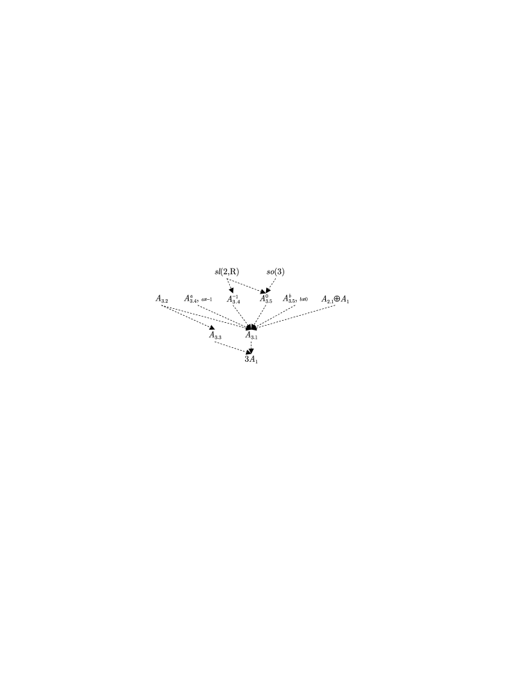
Figure 1: One-parametric contractions of real three-dimensional Lie algebras

Analysis of the obtained results leads to the conclusion that for any pair of real three-dimensional Lie algebras we have one of the two possibilities: 1) there are no contractions in view of applied necessary criteria; 2) there exists a generalized Inönü–Wigner contraction.

Only the contraction $so(3)\xrightarrow{}A_{3.1}$ necessarily is a truly generalized Inönü–Wigner contraction. Nonexistence of a simple Inönü–Wigner contraction in this case is implied by the following chain of statements. Any proper and nontrivial simple Inönü–Wigner contraction corresponds to a proper subalgebra of the initial algebra. Equivalent subalgebras result in equivalent contractions. A complete list of inequivalent proper subalgebras of $so(3)$ is exhausted by any one-dimensional subalgebra of $so(3)$. Any one-dimensional subalgebra generates the contraction of $so(3)$ to $A_{3.5}^{0}$.

All other contractions of real three-dimensional Lie algebras are equivalent to simple Inönü–Wigner contractions although sometimes generalized Inönü–Wigner contraction have a simpler, pure diagonal form. We explicitly indicate two such cases in the above list of contractions, namely, $A_{3.2}\to A_{3.1}$ and $A_{3.2}\to A_{3.3}$.

Note additionally that all the constructed contraction matrices include only nonnegative integer powers of $\varepsilon$, i.e., they admit well-defined limit process under $\varepsilon\to+0$.

Theorem 2.

Any continuous contraction of a real three-dimensional Lie algebra is equivalent to a generalized Inönü–Wigner contraction with nonnegative powers of the contraction parameter. Moreover, only the contraction $so(3)\to A_{3.1}$ is inequivalent to a simple Inönü–Wigner contraction.

8.2 Dimension four

The list of all possible proper and nontrivial continuous one-parametric contractions of real four-dimensional Lie algebras is exhausted by the following ones.

$A_{2.1}\oplus 2A_{1}\colon\quad\xrightarrow{I_{30}W(1,1,0,0)}A_{3.1}\oplus A_{1}$, $\langle e_{3}-e_{1},e_{4}\rangle$.
$2A_{2.1}\colon\quad\xrightarrow{W(0,0,0,1)}A_{2.1}\oplus 2A_{1},\,\langle e_{1},e_{2},e_{3}\rangle;\quad\xrightarrow{I_{1}W(1,1,0,1)}A_{3.1}\oplus A_{1},\,\langle e_{1}+e_{3}\rangle;\quad\\ \hbox{}\qquad\xrightarrow{U_{3}}A_{3.2}\oplus A_{1};\quad\xrightarrow{I_{2}W(0,0,0,1)}A_{3.3}\oplus A_{1},\,\langle e_{1},e_{3},e_{2}+e_{4}\rangle;\quad\xrightarrow{I_{27}W(1,1,0,1)}A^{a}_{3.4}\oplus A_{1},\,\langle e_{2}+ae_{4}\rangle;\\ \hbox{}\qquad\xrightarrow{U_{4}}A_{4.1};\quad\xrightarrow{I_{28}W(0,1,1,0)}A_{4.3},\,\langle e_{1},e_{2}-e_{3}\rangle;\quad\xrightarrow{I_{3}W(1,0,1,0)}A_{4.8}^{0},\,\langle e_{1}+e_{3},e_{2}+e_{4}\rangle$.
$A_{3.2}\oplus A_{1}\colon\quad\xrightarrow{W(1,0,1,0)}A_{3.1}\oplus A_{1},\,\langle e_{2},e_{4}\rangle;\quad\xrightarrow{W(0,1,0,0)}A_{3.3}\oplus A_{1},\,\langle e_{1},e_{3},e_{4}\rangle;\quad\xrightarrow{I_{29}W(2,1,0,1)}A_{4.1}$.
$A_{3.3}\oplus A_{1}\colon\quad\xrightarrow{I_{4}W(1,0,1,0)}A_{3.1}\oplus A_{1},\,\langle e_{1},e_{2}+e_{4}\rangle$.
$A_{3.4}^{a}\oplus A_{1}\colon\quad\xrightarrow{I_{5}W(1,1,0,0)}A_{3.1}\oplus A_{1},\,\langle e_{2},e_{1}+e_{4}\rangle;\quad\xrightarrow{I_{6}W(2,1,0,1)}A_{4.1}$.
$A_{3.5}^{b}\oplus A_{1}\colon\quad\xrightarrow{W(1,0,1,0)}A_{3.1}\oplus A_{1},\,\langle e_{2},e_{4}\rangle;\quad\xrightarrow{I_{9}W(2,1,0,1)}A_{4.1}$.
$sl(2,{\mathbb{R}})\oplus A_{1}\colon\quad\xrightarrow{I_{8}W(1,1,0,0)}A_{3.1}\oplus A_{1},\,\langle e_{3},e_{4}\rangle;\quad\xrightarrow{I_{7}W(1,1,0,0)}A_{3.4}^{-1}\oplus A_{1},\,\langle e_{2},e_{4}\rangle;\quad\\ \hbox{}\qquad\xrightarrow{I_{10}W(1,1,0,0)}A_{3.5}^{0}\oplus A_{1},\,\langle e_{1}+e_{3},e_{4}\rangle;\quad\xrightarrow{I_{23}W(1,1,1,0)}A_{4.1},\,\langle e_{1}+e_{4}\rangle;\\ \hbox{}\qquad\xrightarrow{I_{19}W(1,0,1,0)}A_{4.8}^{-1},\,\langle e_{1},e_{2}-\frac{1}{2}e_{4}\rangle;\quad\xrightarrow{I_{22}W(2,1,1,0)}A_{4.9}^{0}$.
$so(3)\oplus A_{1}\colon\quad\xrightarrow{W(2,1,1,0)}A_{3.1}\oplus A_{1};\quad\xrightarrow{W(1,1,0,0)}A_{3.5}^{0}\oplus A_{1},\,\langle e_{3},e_{4}\rangle;\quad\xrightarrow{I_{5}W(3,2,1,1)}A_{4.1};$ 
  $\xrightarrow{I_{11}W(2,1,1,0)}A_{4.9}^{0}$.
$A_{4.1}\colon\quad\xrightarrow{I_{13}(0)W(0,0,0,1)}A_{3.1}\oplus A_{1},\,\langle e_{1},e_{2},e_{4}\rangle$.
$A_{4.2}^{b}\colon\quad\xrightarrow{I_{14}W(1,0,1,0)}A_{3.1}\oplus A_{1},\,\langle e_{1},e_{3}\rangle;\quad\xrightarrow{b\neq 1,\;I_{15}W(2,1,0,1)}A_{4.1};\quad\xrightarrow{W(1,0,1,0)}A^{b,1,1}_{4.5},\,\langle e_{2},e_{4}\rangle$.
$A_{4.3}\colon\quad\xrightarrow{I_{16}W(0,0,1,0)}A_{2.1}\oplus 2A_{1},\,\langle e_{1},e_{2},e_{4}\rangle;\quad\xrightarrow{I_{14}W(1,0,1,0)}A_{3.1}\oplus A_{1},\,\langle e_{1},e_{3}\rangle;\quad\\ \hbox{}\qquad\xrightarrow{I_{17}W(2,1,0,1)}A_{4.1}$.
$A_{4.4}\colon\quad\xrightarrow{I_{13}(0)W(1,0,1,1)}A_{3.1}\oplus A_{1},\,\langle e_{2}\rangle;\quad\xrightarrow{W(2,1,0,1)}A_{4.1};\quad\xrightarrow{W(0,1,1,0)}A^{1}_{4.2},\,\langle e_{1},e_{4}\rangle;\quad\\ \hbox{}\qquad\xrightarrow{W(0,1,2,0)}A_{4.5}^{111}$.
$A_{4.5}^{ab1}\colon\quad\xrightarrow{a\neq b,\;I_{18}W(1,0,1,0)}A_{3.1}\oplus A_{1},\,\langle\frac{1+b}{a}e_{1}+e_{2},e_{3}\rangle;\quad\xrightarrow{1\neq a\neq b\neq 1,\;I_{12}W(2,1,0,1)}A_{4.1}$.
$A_{4.6}^{ab}\colon\quad\xrightarrow{I_{14}W(1,0,1,0)}A_{3.1}\oplus A_{1},\,\langle e_{1},e_{3}\rangle;\quad\xrightarrow{I_{20}W(2,1,0,1)}A_{4.1}$.
$A_{4.7}\colon\quad\xrightarrow{I_{14}W(1,0,1,0)}A_{3.1}\oplus A_{1},\,\langle e_{1},e_{3}\rangle;\quad\xrightarrow{I_{21}W(1,1,1,0)}A_{4.1},\,\langle e_{4}\rangle;\quad\xrightarrow{W(0,1,1,0)}A_{4.2}^{2},\,\langle e_{1},e_{4}\rangle;\\ \hbox{}\quad\xrightarrow{W(0,0,1,0)}A_{4.5}^{2,1,1},\,\langle e_{1},e_{2},e_{4}\rangle;\quad\xrightarrow{W(1,0,1,0)}A_{4.8}^{1},\,\langle e_{2},e_{4}\rangle$.
$A_{4.8}^{b}\colon\quad\xrightarrow{W(0,0,0,1)}A_{3.1}\oplus A_{1},\,\langle e_{1},e_{2},e_{3}\rangle;$ $\xrightarrow{b=0,\;I_{24}W(0,0,0,1)}A_{3.2}\oplus A_{1},\,\langle e_{1},e_{2},e_{3}+e_{4}\rangle;$
 $\xrightarrow{b=0,\;I_{13}(0)W(0,0,0,1)}A_{3.3}\oplus A_{1},\,\langle e_{1},e_{2},e_{4}\rangle;$ $\xrightarrow{b=-1,\;I_{13}(0)W(1,1,0,1)}A^{-1}_{3.4}\oplus A_{1},\,\langle e_{4}\rangle;$ 
 $\xrightarrow{b\neq 1,\;I_{25}W(1,1,1,0)}A_{4.1},\,\langle e_{2}-e_{3}\rangle;$ $\xrightarrow{-1<b<0,\;W(0,0,1,0)}A_{4.5}^{1+b,1,b},\,\langle e_{1},e_{2},e_{4}\rangle$;
 $\xrightarrow{0<b\leqslant 1,\;\mathop{\rm diag}\nolimits(1,1,1,\frac{1}{1+b})W(0,0,1,0)}A_{4.5}^{1,\frac{1}{1+b},\frac{b}{1+b}},\,\langle e_{1},e_{2},e_{4}\rangle$.
$A_{4.9}^{a}\colon\quad\xrightarrow{W(0,0,0,1)}A_{3.1}\oplus A_{1},\,\langle e_{1},e_{2},e_{3}\rangle;\quad\xrightarrow{a=0,\;I_{14}W(1,1,0,0)}A_{3.5}^{0}\oplus A_{1},\,\langle e_{1},e_{4}\rangle;\quad\\ \hbox{}\quad\xrightarrow{I_{26}W(1,1,1,0)}A_{4.1},\,\langle e_{2}\rangle;\quad\xrightarrow{a\neq 0,\;W(1,1,1,0)}A_{4.6}^{2a,a},\,\langle e_{4}\rangle$.
$A_{4.10}\colon\quad\xrightarrow{I_{13}(0)W(1,0,1,1)}A_{3.1}\oplus A_{1},\,\langle e_{2}\rangle;\quad\xrightarrow{U_{1}}A_{3.2}\oplus A_{1},\quad\xrightarrow{W(0,0,0,1)}A_{3.3}\oplus A_{1},\,\langle e_{1},e_{2},e_{3}\rangle;\quad\\ \hbox{}\quad\xrightarrow{I_{13}W(0,0,0,1)}A_{3.5}^{b}\oplus A_{1},\,\langle e_{1},e_{2},be_{3}+e_{4}\rangle\quad\xrightarrow{U_{2}}A_{4.1},\quad\xrightarrow{I_{13}(0)W(1,0,1,0)}A_{4.8}^{0},\,\langle e_{2},e_{3}\rangle$.

The constant parts of matrices of generalized Inönü–Wigner contractions have the form

$$I_{1}=\left(\begin{array}[]{cccc}0&0&1&0\\ 0&0&0&1\\ -1&0&1&0\\ 0&1&0&1\\ \end{array}\right), I_{2}=\left(\begin{array}[]{cccc}1&2&0&0\\ 0&0&1&0\\ 0&1&0&0\\ 0&0&1&1\\ \end{array}\right), I_{3}=\left(\begin{array}[]{cccc}0&-1&0&0\\ 0&0&0&1\\ -1&-1&0&0\\ 0&0&1&1\\ \end{array}\right),$$

$$I_{4}=\left(\begin{array}[]{cccc}0&0&0&1\\ -1&-1&0&0\\ 0&0&1&0\\ 0&-1&0&0\\ \end{array}\right), I_{5}=\left(\begin{array}[]{cccc}-1&0&1&0\\ 0&0&0&1\\ 0&1&0&0\\ 0&0&1&0\\ \end{array}\!\!\right),\; I_{6}=\left(\begin{array}[]{cccc}-\frac{1}{a}&\frac{1}{a(a-1)}&\frac{1}{a(a-1)}&0\\ 0&a&1&0\\ 0&0&0&1\\ 0&0&1&0\\ \end{array}\right),$$

$$I_{7}=\left(\begin{array}[]{cccc}1&0&0&0\\ 0&0&1&0\\ 0&-1&0&0\\ 0&0&0&1\\ \end{array}\right), I_{8}=\left(\begin{array}[]{cccc}0&1&0&0\\ 2&0&0&0\\ 0&0&1&0\\ 0&0&0&1\\ \end{array}\right), I_{9}=\left(\begin{array}[]{cccc}1&0&\frac{-1}{b^{2}+1}&0\\ 0&1&\frac{b}{b^{2}+1}&0\\ 0&0&0&1\\ 0&0&1&0\\ \end{array}\right),$$

$$I_{10}=\left(\begin{array}[]{cccc}0&0&\frac{1}{2}&0\\ 0&1&0&0\\ 1&0&\frac{1}{2}&0\\ 0&0&0&1\\ \end{array}\right), I_{11}=\left(\begin{array}[]{cccc}1&0&0&1\\ 0&1&0&0\\ 0&0&1&0\\ 0&0&0&1\\ \end{array}\right), I_{12}=\left(\!\!\!\!\!\!\begin{array}[]{cccc}\frac{1}{b-1}&\frac{(a-b)^{-1}}{(b-1)}&\frac{(a-b)^{-1}}{(a-1)(b-1)}\!\!\!\!\!&0\\ 0&b-1&1&0\\ 0&0&1&0\\ 0&0&0&1\\ \end{array}\!\!\!\right),$$

$$I_{13}(b)=\left(\begin{array}[]{cccc}1&0&0&0\\ 0&1&0&0\\ 0&0&b&1\\ 0&0&1&0\\ \end{array}\right), I_{14}=\left(\begin{array}[]{cccc}0&0&0&1\\ 1&0&0&0\\ 0&1&0&0\\ 0&0&1&0\\ \end{array}\right), I_{15}=\left(\begin{array}[]{cccc}1&\frac{-1}{b-1}&\frac{-1}{(b-1)^{2}}&0\\ 0&1&0&0\\ 0&0&1&0\\ 0&0&0&1\\ \end{array}\right),$$

$$I_{16}=\left(\begin{array}[]{cccc}1&0&0&0\\ 0&0&0&1\\ 0&0&1&0\\ 0&1&0&0\\ \end{array}\right), I_{17}=\left(\begin{array}[]{cccc}1&1&1&0\\ 0&1&0&0\\ 0&0&1&0\\ 0&0&0&1\\ \end{array}\right), I_{18}=\left(\begin{array}[]{cccc}1&\frac{1+b}{a}&0&0\\ 0&1&0&0\\ 0&0&0&1\\ 0&0&1&0\\ \end{array}\right),$$

$$I_{19}=\left(\begin{array}[]{cccc}0&1&0&0\\ 0&0&0&1\\ 0&0&1&0\\ 1&0&0&-\tfrac{1}{2}\\ \end{array}\right), I_{20}=\left(\!\begin{array}[]{cccc}-1&0&0&0\\ 0&1&0&0\\ 0&0&0&-1\\ 0&0&1&0\\ \end{array}\!\!\right)\!,\; I_{21}=\left(\!\!\!\begin{array}[]{cccc}1&\!\frac{(a-b)(a-1)\!^{-1}}{a-b+1}\!&\!\frac{(a-1)\!^{-1}}{a-b+1}\!&0\\ 0&0&1&0\\ 0&-1&0&0\\ 0&0&0&1\\ \end{array}\!\!\!\right)\!,\;$$

$$I_{22}=\left(\begin{array}[]{cccc}-\frac{1}{2}&0&\frac{1}{2}&\frac{1}{2}\\ 0&1&0&0\\ -\frac{1}{2}&0&-\frac{1}{2}&\frac{1}{2}\\ 0&0&0&1\\ \end{array}\right),\ \ I_{23}=\left(\begin{array}[]{cccc}0&0&0&1\\ 0&1&0&0\\ 0&0&-\tfrac{1}{2}&0\\ 1&0&0&1\\ \end{array}\right),\ \ I_{24}=\left(\begin{array}[]{cccc}1&0&0&0\\ 0&1&0&0\\ 0&0&1&0\\ 0&0&1&1\\ \end{array}\right),$$

$$I_{25}=\left(\begin{array}[]{cccc}1&0&0&0\\ 0&1&0&-1\\ 0&0&0&1\\ 0&0&\frac{1}{b-1}&0\\ \end{array}\right), I_{26}=\left(\begin{array}[]{cccc}-1&0&0&0\\ 0&0&0&1\\ 0&1&0&0\\ 0&0&1&0\\ \end{array}\right), I_{27}=\left(\begin{array}[]{cccc}1&0&0&0\\ 0&0&1&0\\ 0&1&0&0\\ 0&0&a&-1\\ \end{array}\right),$$

$$I_{28}=\left(\begin{array}[]{cccc}-1&0&0&0\\ 0&0&0&1\\ 0&1&0&-1\\ 0&0&1&0\end{array}\right), I_{29}=\left(\begin{array}[]{cccc}1&0&-1&0\\ 0&1&1&0\\ 0&0&0&1\\ 0&0&1&0\end{array}\right), I_{30}=\left(\begin{array}[]{cccc}1&0&-1&0\\ 0&1&0&0\\ 0&0&1&0\\ 0&0&0&1\end{array}\right).$$

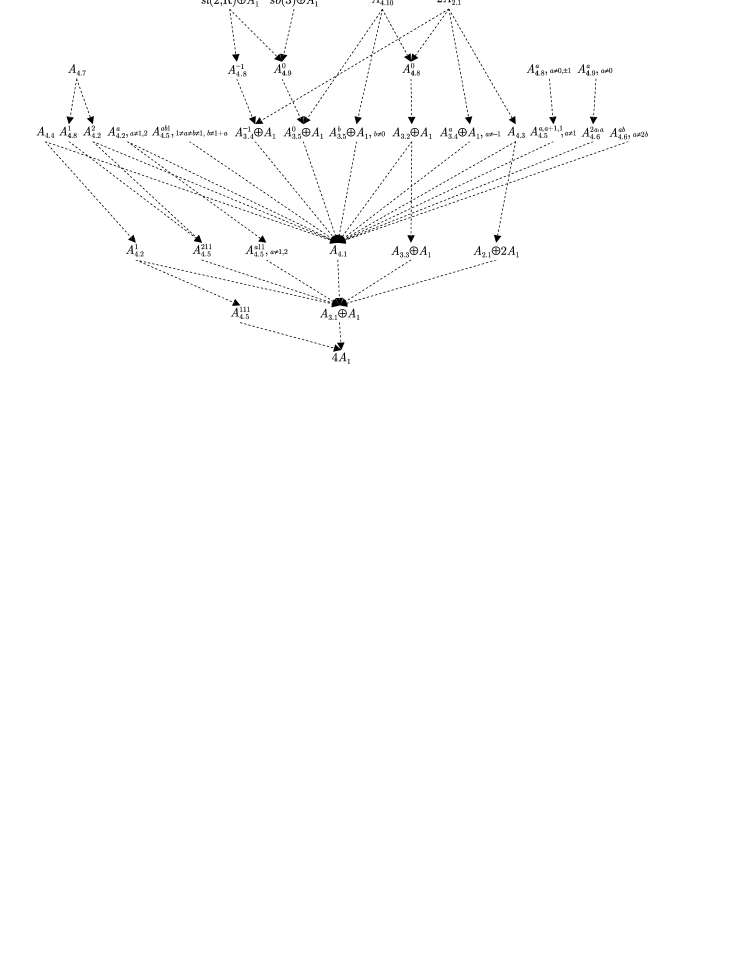
Figure 2: One-parametric contractions of real four-dimensional Lie algebras

Remark 10.

All the constructed contraction matrices include only nonnegative integer powers of $\varepsilon$. Therefore, they admit well-defined limit process under $\varepsilon\to+0$. Moreover, most contractions are equivalent to simple IW-contractions.

All generalized IW-contractions of solvable real four-dimensional algebras (namely, $A_{3.2}\oplus A_{1}$, $A_{3.4}^{a}\oplus A_{1}$, $A_{3.5}^{b}\oplus A_{1}$, $A_{4.2}^{b}$, $b{\neq}1$, $A_{4.3}$, $A_{4.4}$, $A_{4.5}^{ab1}$, $1{\neq}a{\neq}b{\neq}1$, $A_{4.6}^{ab}$) to $A_{4.1}$ are direct and, therefore, cannot be presented via composition of simple IW-contractions. The same statement is true for the contractions of the unsolvable algebras ($sl(2,{\mathbb{R}})\oplus A_{1}$ and $so(3)\oplus A_{1}$) to $A_{4.9}^{0}$. Only three generalized IW-contractions ($so(3)\oplus A_{1}\to A_{3.1}\oplus A_{1}$, $so(3)\oplus A_{1}\to A_{4.1}$ and $A_{4.4}\to A_{4.5}^{111}$) are decomposed to sequences of simple IW-contractions. The listed contractions exhaust a set of inequivalent ‘truly’ generalized IW-contractions of the real four-dimensional algebras.

In contrast to three-dimensional Lie algebras, there exist four contractions of four-dimensional Lie algebras, which are inequivalent to generalized Inönü–Wigner contractions, namely

$$A_{4.10}\xrightarrow{U_{1}}A_{3.2}\oplus A_{1},\quad 2A_{2.1}\xrightarrow{U_{2}}A_{3.2}\oplus A_{1},$$

$$A_{4.10}\xrightarrow{U_{3}}A_{4.1},\quad 2A_{2.1}\xrightarrow{U_{4}}A_{4.1},$$

They are provided by the ‘non-diagonalizable’ matrices

$$U_{1}=\left(\begin{array}[]{cccc}\varepsilon&0&0&0\\ 0&1&0&0\\ 0&0&1&\varepsilon\\ 0&0&\varepsilon&0\end{array}\right),\quad U_{2}=\left(\begin{array}[]{cccc}0&-1&0&0\\ 0&0&1&\varepsilon\\ -\varepsilon&-1&0&0\\ 0&0&1+\varepsilon&\varepsilon\end{array}\right),$$

$$U_{3}=\left(\begin{array}[]{cccc}\varepsilon^{2}&0&0&0\\ 0&\varepsilon&0&-1\\ 0&0&\varepsilon&0\\ 0&0&0&\varepsilon\end{array}\right),\quad U_{4}=\left(\begin{array}[]{cccc}-\varepsilon^{2}&-\varepsilon&-1&-1\\ 0&0&\varepsilon&0\\ 0&-\varepsilon^{2}&-\varepsilon&0\\ 0&0&\varepsilon&\varepsilon\end{array}\right).$$

The matrices $U_{1}$ and $U_{2}$ include only the zero and first powers of the contraction parameter. Therefore, the corresponding contractions are Saletan ones.

Remark 11.

The maximal powers of contraction parameter, which are in components of contraction matrices, can be lowered if the restriction with the class of generalized IW-contractions in the case they exist will be neglected. For example, a generalized IW-contraction from the algebra $so(3)\oplus A_{1}$ to $A_{4.9}^{0}$ is generated by the matrix $I_{11}W(2,1,1,0)$ containing components with the second power of the contraction parameter. At the same time, it is known [67] that there exist the Saletan contraction between these algebras which is provided by the matrix

$$\left(\begin{array}[]{cccc}0&\varepsilon&0&0\\ 0&0&\varepsilon&0\\ -\varepsilon&0&0&1\\ -\varepsilon&0&0&1-\varepsilon\end{array}\right)$$

obviously being of the first power with respect to $\varepsilon$.

Another example is given by the contraction $so(3)\oplus A_{1}\to A_{4.1}$. It is generated, as a generalized IW-contraction, with the matrix $I_{5}W(3,2,1,1)$ and has the essential contraction parameter power which is equal to 3 and is maximal among the generalized IW-contractions of the four-dimensional Lie algebras. All the other presented generalized IW-contractions contain at most the second power of the contraction parameter. (The similar situation is in the three-dimensional case where the unique truly generalized IW-contraction is the contraction $so(3)\to A_{3.1}$ with the matrix $W(2,1,1)$ containing the second power of $\varepsilon$.) The matrix $I_{5}W(3,2,1,1)$ can be replaced with the matrix

$$\left(\begin{array}[]{cccc}0&0&\varepsilon&0\\ 0&-\varepsilon^{2}&0&0\\ 0&0&0&\varepsilon\\ -\varepsilon^{2}&0&-1&0\end{array}\right)$$

which has no ‘generalized IW-form’ and contains at most the second power of the contraction parameter.

Remark 12.

In each from the following pairs of Lie algebras

$$(so(3)\oplus A_{1},\,A_{4.8}^{-1}),\quad(so(3)\oplus A_{1},\,A_{3.4}^{-1}\oplus A_{1}),\quad(A_{4.8}^{-1},\,A_{3.5}^{0}\oplus A_{1}),\quad(A_{4.9}^{0},\,A_{3.4}^{-1}\oplus A_{1}),$$

$$(A_{4.10},\,A_{4.3}),\quad(A_{4.10},\,A_{2.1}\oplus 2A_{1}),\quad(A_{4.10},\,A^{a}_{3.4}\oplus A_{1}),\quad(2A_{2.1},\,A^{b}_{3.5}\oplus A_{1}),$$

the first algebra is contracted to the second one over the complex field. See Section 9 additionally. In particular,

$$A_{4.10}\xrightarrow{I_{31}W(1,1,1,0)}A_{4.3},\quad A_{4.10}\xrightarrow{I_{32}W(1,1,0,1)}A_{3.4}^{a}\oplus A_{1},\quad 2A_{2.1}\xrightarrow{I_{33}W(0,0,0,1)}A^{b}_{3.5}\oplus A_{1},$$

where

$$I_{31}=\left(\begin{array}[]{cccc}-i&i&0&-i\\[1.93748pt] 1&1&0&-1\\[1.93748pt] 0&0&\frac{1}{2}&\frac{1}{2}\\[1.93748pt] 0&0&\frac{1}{2}&-\frac{i}{2}\\[1.93748pt] \end{array}\right),\;I_{32}=\left(\begin{array}[]{cccc}i&-1&0&0\\[1.93748pt] i&1&0&0\\[1.93748pt] 0&0&\frac{1+a}{2}&\frac{-i(1+a)}{2}\\[1.93748pt] 0&0&-\frac{1}{2}&-\frac{i}{2}\\[1.93748pt] \end{array}\right),\;I_{33}=\left(\begin{array}[]{cccc}-\frac{i}{2}&-\frac{1}{2}&0&0\\[1.93748pt] 0&0&b+i&1\\[1.93748pt] -\frac{i}{2}&\frac{1}{2}&0&0\\[1.93748pt] 0&0&b-i&1\end{array}\right).$$

Therefore, almost all necessary criteria hold true since they do not discriminate between the real and complex fields. At the same time, there are no real contractions in these pairs. To prove it, we have to apply criteria specific for the real numbers, e.g., Criterion 16 which is based on the law of inertia of quadratic forms over the real field.

For the first four pairs it is enough to consider only their Killing forms. $\kappa_{so(3)\oplus A_{1}}=-2(u_{1}v_{1}+u_{2}v_{2}+u_{3}v_{3})$, $\kappa_{A_{3.5}^{0}\oplus A_{1}}=-2u_{3}v_{3}$ and $\kappa_{A_{4.9}^{0}}=-2u_{4}v_{4}$ are nonpositively defined. $\kappa_{A_{4.8}^{-1}}=2u_{4}v_{4}$ and $\kappa_{A_{3.4}^{-1}\oplus A_{1}}=2u_{3}v_{3}$ are nonnegatively defined. All the above forms do not vanish identically. Therefore, in each of these pairs an algebra has the nonpositively defined nonzero Killing form and the other does the nonnegative defined nonzero one. In view of necessary Criterion 16, there are no contractions in these pairs.

The criterion based on inertia of the Killing forms is powerless for the algebras from the other pairs. For them we consider the modified Killing forms with the specially chosen value $\alpha=-1/2$:

$$\tilde{\kappa}_{A_{4.10}}^{-1/2}=2(1+2\alpha)u_{3}v_{3}-2u_{4}v_{4}\big{|}_{\alpha=-1/2}=-2u_{4}v_{4},$$

$$\tilde{\kappa}_{A_{3.5}^{b}\oplus A_{1}}^{-1/2}=2((1+2\alpha)b^{2}-1)u_{3}v_{3}\big{|}_{\alpha=-1/2}=-2u_{3}v_{3},$$

$$\tilde{\kappa}_{A_{4.3}}^{-1/2}=(1+\alpha)u_{4}v_{4}\big{|}_{\alpha=-1/2}=\frac{1}{2}u_{2}v_{2},\qquad\tilde{\kappa}_{A_{2.1}\oplus 2A_{1}}^{-1/2}=(1+\alpha)u_{2}v_{2}\big{|}_{\alpha=-1/2}=\frac{1}{2}u_{4}v_{4},$$

$$\tilde{\kappa}_{A_{3.4}^{a}\oplus A_{1}}^{-1/2}=((1+a^{2})+\alpha(1+a)^{2})u_{3}v_{3}\big{|}_{\alpha=-1/2}=\frac{1}{2}(1-a+a^{2})u_{3}v_{3},$$

$$\tilde{\kappa}_{2A_{2.1}}^{-1/2}=((1{+}\alpha)(u_{2}v_{2}{+}u_{4}v_{4})+\alpha(u_{2}v_{4}{+}u_{4}v_{2}))\big{|}_{\alpha=-1/2}=\frac{1}{2}((u_{2}v_{2}{+}u_{4}v_{4})-(u_{2}v_{4}{+}u_{4}v_{2})).$$

Two first forms are nonpositively defined and nonzero. The others are nonnegatively defined and also do not vanish identically. In view of the second part of Criterion 16, there are no contractions in the pairs under consideration.

8.3 Levels and colevels of low-dimensional real Lie algebras

Contractions assign the partial ordering relationship on the variety $\mathcal{L}_{n}$ of $n$-dimensional Lie algebras. Namely, we assume that $\mathfrak{g}\succ\mathfrak{g}_{0}$ if $g_{0}$ is a proper contraction of $g$. The introduced strict order is well defined due to the transitivity property of contractions. If improper contractions are allowed in the definition of ordering then the partial ordering becomes nonstrict.

The order $\succ$ generates separation of $\mathcal{L}_{n}$ to tuples of levels of different types.

Definition 7.

The Lie algebra $\mathfrak{g}$ from $\mathcal{L}_{n}$ belongs to the zero level of $\mathcal{L}_{n}$ if it has no proper contractions. The other levels of $\mathcal{L}_{n}$ are defined by induction. The Lie algebra $\mathfrak{g}$ belongs to $k$-level of $\mathcal{L}_{n}$ if it can be contracted to algebras from $(k-1)$-level and only to algebras from the previous levels.

Remark 13.

We have recently become aware due to [47] that the notion of level was introduced and investigated by Gorbatsevich [27, 28, 29]. He also proposed another notion of level based on interesting generalization of contractions to case of different dimensions of initial and contracted algebras, which is reviewed in the Introduction.

The zero level of $\mathcal{L}_{n}$ for any $n$ contains exactly one algebra, and it is the $n$-dimensional Abelian algebra which is the unique minimal element in $\mathcal{L}_{n}$. The elements of the last level are maximal elements with respect to the ordering relationship induced by contractions in $\mathcal{L}_{n}$ but do not generally exhaust the set of maximal elements of $\mathcal{L}_{n}$.

Obtained exhaustive description of contractions of low-dimensional Lie algebras allows us to study completely levels of these algebras.

$\mathcal{L}_{1}$ consists of one element and has only one algebra level. Analogously, $\mathcal{L}_{2}$ is formed by two elements and is separated by contractions into exactly two levels. The first level consists of the two-dimensional non-Abelian algebra $A_{2.1}$ and the zero level does the two-dimensional Abelian algebra $2A_{1}$.

The hierarchies of levels of real three- and four-dimensional Lie algebras are more complicated. Actually, they are already represented in Figures 1 and 2, where the level number grows upward. It is the usage of the level ideology that makes the figures clear and elucidative. $\mathcal{L}_{3}$ and $\mathcal{L}_{4}$ have four and six levels, correspondingly.

Remark 14.

Structure of Lie algebra is simplified under contraction. The level number of an algebra can be assumed as a measure of complexity of its commutation structure, i.e., algebras with higher level numbers are more complicated than those with lower level numbers. In particular, nilpotent algebras are in low levels. The simple algebras $sl(2,{\mathbb{R}})$ and $so(3)$ having the most complicated structures among three-dimensional algebras form the highest 3-level of $\mathcal{L}_{3}$. The highest 6-level of $\mathcal{L}_{4}$ is formed by the unsolvable algebras $sl(2,{\mathbb{R}})\oplus A_{1}$ and $so(3)\oplus A_{1}$ and the perfect (by Jacobson [44]) algebras $2A_{2.1}$ and $A_{4.10}$.

Remark 15.

There exists an inverse correlation of level numbers with dimensions of differentiation algebras (or a direct correlation with dimensions of algebra orbits), which is connected with necessary Criterion 1. As a rule, the algebras with the same dimension of differentiation algebras belong to the same level. The dimensions of differentiation algebras of the algebras from $k$-level are not less and generally greater than those of the algebras from $(k+1)$-level.

For the three-dimensional Lie algebras the correlation is complete. Namely, the dimensions of differentiation algebras take the values of 9, 6, 4, 3 for the algebras from 0-, 1-, 2- and 3-level, correspondingly.

In $\mathcal{L}_{4}$ the correlation is partially broken. Namely, for almost all algebras from $3$-level the dimensions of the differentiation algebras equal to six and only the algebra $A^{1}_{4.8}$ which also belongs to this level has seven-dimensional differentiation algebra. The same happens in $2$-level. Almost all algebras have eight-dimensional differentiation algebras except the algebra $A_{4.1}$ with seven-dimensional differentiation algebra. In other words, the four-dimensional Lie algebras with $\dim\mathop{\rm Der}\nolimits=7$ are separated between the second and third levels, and the ‘simpler’ nilpotent algebra $A_{4.1}$ belongs to the lower level. The algebras $A_{4.5}^{111}$ ($\dim\mathop{\rm Der}\nolimits=12$) and $A_{3.1}\oplus A_{1}$ ($\dim\mathop{\rm Der}\nolimits=10$) form 1-level. In all other cases the correlation is complete. 0-, 5- and 6-levels consist of the algebras having 16-, 5- and 4-dimensional differentiation algebras correspondingly.

Starting from the Lie algebras which are not proper contractions of any Lie algebras, we can introduce the related definition of colevel.

Definition 8.

The Lie algebra $\mathfrak{g}$ from $\mathcal{L}_{n}$ belongs to the zero colevel of $\mathcal{L}_{n}$ if it is not a proper contraction of any $n$-dimensional Lie algebra. The other colevels of $\mathcal{L}_{n}$ are defined by induction. The Lie algebra $\mathfrak{g}$ belongs to a colevel of $\mathcal{L}_{n}$ if it is a proper contraction only of algebras from the previous colevels.

0-colevel coincides with the set of maximal elements with respect to the order induced by contractions in $\mathcal{L}_{n}$, i.e., it is formed by the algebras which are not proper contractions of the other algebras from $\mathcal{L}_{n}$. The last colevel of $\mathcal{L}_{n}$ for any $n$ contains exactly one algebra, and it is the $n$-dimensional Abelian algebra.

For the lowest dimensions structures of levels and colevels are analogous. $\mathcal{L}_{1}$ has only 0-colevel which obviously coincides with 0-level. $\mathcal{L}_{2}$ is separated by contractions into exactly two colevels. The zero and first colevels coincide with the first and zero levels, correspondingly.

The hierarchies of colevels of real three- and four-dimensional Lie algebras differ from the hierarchies of levels and adduced below.

Colevels of three-dimensional algebras:

1. $A_{2.1}\oplus A_{1}$, $A_{3.2}$, $A_{3.4}^{a}$, $a\neq-1$, $A_{3.5}^{b}$, $b\neq 0$, $sl(2,{\mathbb{R}})$, $so(3)$;

2. $A_{3.3}$, $A_{3.4}^{-1}$, $A_{3.5}^{0}$;

3. $A_{3.1}$;

4. $3A_{1}$.

Colevels of four-dimensional algebras:

1. $2A_{2.1}$, $sl(2,{\mathbb{R}})\oplus A_{1}$, $so(3)\oplus A_{1}$, $A_{4.2}^{b}$, $b\neq 1,2$, $A_{4.4}$, $A_{4.6}^{ab}$, $a\neq 2b$, $A_{4.7}$, $A_{4.8}^{b}$, $b\neq 0,\pm 1$, $A_{4.9}^{a}$, $a\neq 0$, $A_{4.10}$, $A_{4.5}^{abc}$, $a\neq b\neq c\neq a,\,b\neq a+1$;

2. $A_{3.4}^{a}\oplus A_{1}$, $a\neq-1$, $A_{3.5}^{b}\oplus A_{1}$, $b\neq 0$, $A_{4.2}^{1}$, $A_{4.2}^{2}$, $A_{4.3}$, $A_{4.5}^{a,a+1,1}$, $a\neq 1$, $A_{4.5}^{a11}$, $a\neq 1,2$, $A_{4.6}^{2b,b}$, $A_{4.8}^{-1}$, $A_{4.8}^{0}$, $A_{4.8}^{1}$, $A_{4.9}^{0}$;

3. $A_{2.1}\oplus 2A_{1}$, $A_{3.2}\oplus A_{1}$, $A_{3.4}^{-1}\oplus A_{1}$, $A_{3.5}^{0}\oplus A_{1}$, $A_{4.5}^{111}$, $A_{4.5}^{211}$;

4. $A_{3.3}\oplus A_{1}$, $A_{4.1}$;

5. $A_{3.1}\oplus A_{1}$;

6. $4A_{1}$.

Remark 16.

The levels and colevels of $\mathcal{L}_{n}$ are related. The numbers of levels and colevels of $\mathcal{L}_{n}$ coincide and equal to the maximal length of chains of direct contractions. If a fixed Lie algebra $\mathfrak{g}$ from $\mathcal{L}_{n}$ belongs to $k_{1}$-level and $k_{2}$-colevel then $k_{1}+k_{2}\leqslant n^{2}-n$.

Remark 17.

Correlation of co-level numbers with dimensions of differentiation algebras (or orbit dimensions) is essentially weaker than for level numbers. For each separated part of series of Lie algebras the orbit dimension of the whole part should be used here. It equals the sum of orbit dimension of single algebras from this part and the number of essential parameters parameterizing this part. Even for the three-dimensional Lie algebras the correlation is broken in some cases. For example, the orbit dimensions of the algebras $A_{3.1}$ and $A_{3.3}$ equal to three and they belong to different co-levels. In spite of such weak correlation, the notion of co-level is useful in studying geometrical structure of $\mathcal{L}_{n}$. In particular, more regular (i.e., having less constraints on parameters) parts of series of Lie algebras have less co-level numbers than more singular ones.

Analyzing obtained results for dimensions three and four, we induce a number of conjectures. Testing and proof of them are out of the subject of this paper. We have recently learned that some of them are already proved [27, 47]. We unite known statements in the following theorem. Let $\mathfrak{a}_{E_{n-1}}$ be the almost Abelian algebra which contains an $(n-1)$-dimensional Abelian ideal and an element the adjoint action of which on the ideal is the identical operator $E_{n-1}$.

Theorem 3.

For any $n>2$ 1-level of $\mathcal{L}_{n}$ is formed by the algebras $A_{3.1}\oplus(n-3)A_{1}$ and $\mathfrak{a}_{E_{n-1}}$.

9 One-parametric contractions of complex low-dimensional
Lie algebras

Some algebras which are inequivalent over the real field could be representatives of the same class of algebras over the complex field.

Below we list pairs of real three- and four-dimensional Lie algebras which are isomorphic or belong to the same series over the complex field. For each of them we present the corresponding complex algebra (or series) together with the appropriate basis transformation in the case it is non-identical. The list is completed by the pairs of the direct sums $(A_{3.4}^{a}\oplus A_{1},A_{3.5}^{b}\oplus A_{1})$ and $(sl(2,{\mathbb{R}})\oplus A_{1},so(3)\oplus A_{1})$ isomorphisms of which become obvious. Any complex indecomposable solvable algebra is denoted by $\mathfrak{g}_{n.k}$, where $n$ is the dimension of the algebra and $k$ is the number of the real algebra with the same form of canonical commutation relations.

$$\begin{array}[]{ll}\lx@intercol\@ADDCLASS{ltx_eqn_lefteqn}$\displaystyle\begin{array}[]{l}\mathfrak{g}_{3.4}^{\alpha},\\ \alpha\in{\mathbb{C}}\end{array}$\mbox{}\hfil\lx@intercol\phantom{sl(2,{{\mathbb{C}}})}&\left\{\begin{array}[]{ll}A_{3.5}^{b},&\tilde{e}_{1}=e_{1}+ie_{2},\;\tilde{e}_{2}=e_{1}-ie_{2},\;\tilde{e}_{3}=\frac{1}{b+i}e_{3},\;\alpha=\frac{b-i}{b+i}\\[4.30554pt] A_{3.4}^{a},&\alpha=a\end{array}\right.\end{array}$$

$$\begin{array}[]{ll}sl(2,{{\mathbb{C}}})&\left\{\begin{array}[]{ll}so(3),&\tilde{e}_{1}=-ie_{2}+e_{3},\;\tilde{e}_{2}=-ie_{1},\;\tilde{e}_{3}=ie_{2}+e_{3}\\[4.30554pt] sl(2,{\mathbb{R}})&\end{array}\right.\end{array}$$

$$\begin{array}[]{ll}\lx@intercol\@ADDCLASS{ltx_eqn_lefteqn}$\displaystyle\begin{array}[]{l}\mathfrak{g}_{4.5}^{1,\alpha,\beta},\\ \alpha,\beta\in{\mathbb{C}}\end{array}$\mbox{}\hfil\lx@intercol\phantom{sl(2,{{\mathbb{C}}})}&\left\{\begin{array}[]{ll}A_{4.6}^{a,b},&\tilde{e}_{1}=e_{1},\;\tilde{e}_{2}=e_{2}-ie_{3},\;\tilde{e}_{3}=e_{2}+ie_{3},\;\tilde{e}_{4}=\frac{1}{a}e_{4},\;\alpha=\frac{b-i}{a},\;\beta=\frac{b+i}{a}\\[4.30554pt] A_{4.5}^{1,b,c},&\alpha=b,\;\beta=c\end{array}\right.\end{array}$$

$$\begin{array}[]{ll}\lx@intercol\@ADDCLASS{ltx_eqn_lefteqn}$\displaystyle\begin{array}[]{l}\mathfrak{g}_{4.8}^{\beta},\\ \beta\in{\mathbb{C}}\end{array}$\mbox{}\hfil\lx@intercol\phantom{sl(2,{{\mathbb{C}}})}&\left\{\begin{array}[]{ll}A_{4.9}^{a},&\tilde{e}_{1}=-e_{1},\;\tilde{e}_{2}=e_{2}+ie_{3},\;\tilde{e}_{3}=-\frac{i}{2}e_{2}-\frac{1}{2}e_{3},\;\tilde{e}_{4}=\frac{1}{a+i}e_{4},\;\beta=\frac{a-i}{a+i}\\[4.30554pt] A_{4.8}^{b},&\beta=b\end{array}\right.\end{array}$$

$$\begin{array}[]{ll}\lx@intercol\@ADDCLASS{ltx_eqn_lefteqn}$\displaystyle 2\mathfrak{g}_{2.1}$\mbox{}\hfil\lx@intercol\phantom{sl(2,{{\mathbb{C}}})}&\left\{\begin{array}[]{ll}A_{4.10},&\tilde{e}_{1}=ie_{1}-e_{2},\;\tilde{e}_{2}=\frac{1}{2}e_{3}-\frac{i}{2}e_{4},\;\tilde{e}_{3}=ie_{1}+e_{2},\;\tilde{e}_{4}=\frac{1}{2}e_{3}+\frac{i}{2}e_{4}\\[4.30554pt] 2A_{2.1}&\end{array}\right.\end{array}$$

Knowledge of the correspondences between real and complex Lie algebras allows us to describe all continuous contractions of the complex low-dimensional Lie algebras. The corresponding lists are produced from the analogous lists for the real low-dimensional Lie algebras by accurate elimination of algebras which are equivalent to other forms over the complex field. The contraction matrices are preserved. The contractions of three- and four-dimensional complex algebras are visualized with Figure 3 and Figure 4. The one- and two-dimensional cases are trivial and are not considered.

Figure 3: One-parametric contractions of three-dimensional complex Lie algebras

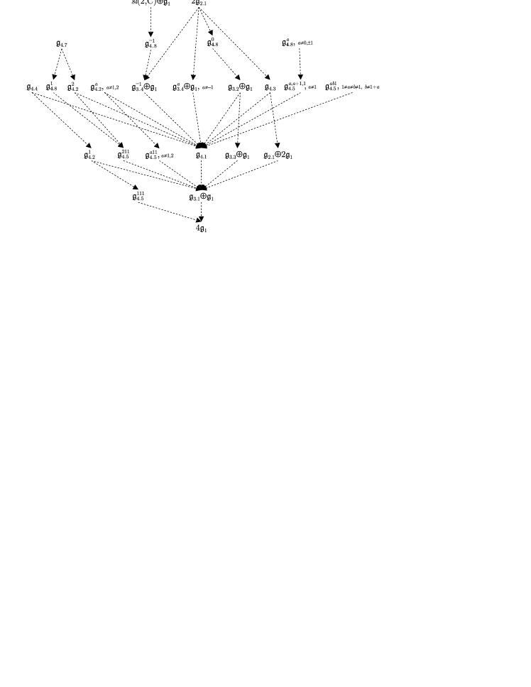
Figure 4: One-parametric contractions of four-dimensional complex Lie algebras

Theorem 4.

Any continuous contraction of complex three-dimensional Lie algebras is equivalent to a simple Inönü–Wigner contraction.

In four-dimensional case only the contractions $2\mathfrak{g}_{2.1}\to\mathfrak{g}_{3.2}\oplus\mathfrak{g}_{1}$ and $2\mathfrak{g}_{2.1}\to\mathfrak{g}_{4.1}$ are not presented as generalized Inönü–Wigner contractions. All the constructed contraction matrices include only nonnegative integer powers of $\varepsilon$. Therefore, they admit well-defined limit process under $\varepsilon\to+0$.

A list of continuous contractions of the complex three-dimensional Lie algebras was adduced, e.g., in [1, 9, 71] in terms of orbit closures. It obviously coincides with that presented in Figure 3. In [9, 71] and later in [2] contractions of the four-dimensional complex Lie algebras are also investigated. Comparing these results with ours, at first we determine correspondence between the used lists of algebras. To avoid confusions, we add hats over the symbol $\mathfrak{g}$ denoting algebras from [9]. Note also that the list used in [9] is essentially based on classification obtained in [63].

$$\begin{array}[t]{ll}4\mathfrak{g}_{1}\sim{\mathbb{C}}^{4};&\mathfrak{g}_{4.1}\sim\mathfrak{n}_{4};\\[1.72218pt] \mathfrak{g}_{2.1}\oplus 2\mathfrak{g}_{1}\sim\mathfrak{r}_{2}\oplus{\mathbb{C}}^{2};&\mathfrak{g}_{4.2}^{1}\sim\hat{\mathfrak{g}}_{5};\ \mathfrak{g}_{4.2}^{-2}\sim\hat{\mathfrak{g}}_{3}\Bigl{(}\frac{27}{4}\Bigr{)};\ \mathfrak{g}_{4.2}^{b\neq 1,-2}\sim\hat{\mathfrak{g}}_{2}\Bigl{(}\frac{b}{(b+2)^{3}},\frac{2b+1}{(b+2)^{2}}\Bigr{)};\\[4.73611pt] 2\mathfrak{g}_{2.1}\sim\mathfrak{r}_{2}\oplus\mathfrak{r}_{2};&\mathfrak{g}_{4.3}\sim\hat{\mathfrak{g}}_{2}(0,0);\\[4.73611pt] \mathfrak{g}_{3.1}\oplus\mathfrak{g}_{1}\sim\mathfrak{n}_{3}\oplus{\mathbb{C}};&\mathfrak{g}_{4.4}\sim\hat{\mathfrak{g}}_{2}(\frac{1}{27},\frac{1}{3});\\[4.73611pt] \mathfrak{g}_{3.2}\oplus\mathfrak{g}_{1}\sim\mathfrak{r}_{3}\oplus{\mathbb{C}};&\mathfrak{g}_{4.5}^{a11}\sim\hat{\mathfrak{g}}_{1}(a);\\[4.73611pt] \mathfrak{g}_{3.3}\oplus\mathfrak{g}_{1}\sim\mathfrak{r}_{3,1}\oplus{\mathbb{C}};&\mathfrak{g}_{4.5}^{ab1}\sim\hat{\mathfrak{g}}_{2}(\alpha,\beta),\hat{\mathfrak{g}}_{3}(\gamma),\hat{\mathfrak{g}}_{4},\ \mbox{\scriptsize$1\neq a\neq b\neq 1,\ ab\neq 0$};\\[4.73611pt] \mathfrak{g}_{3.4}^{a}\oplus\mathfrak{g}_{1}\sim\mathfrak{r}_{3,a}\oplus{\mathbb{C}},\ \mbox{\scriptsize$a\neq 1$};&\mathfrak{g}_{4.7}\sim\hat{\mathfrak{g}}_{8}(\frac{1}{4});\\[3.44444pt] sl(2,{\mathbb{C}})\oplus\mathfrak{g}_{1}\sim sl_{2}({\mathbb{C}})\oplus{\mathbb{C}};&\mathfrak{g}_{4.8}^{1}\sim\hat{\mathfrak{g}}_{6};\ \mathfrak{g}_{4.8}^{-1}\sim\hat{\mathfrak{g}}_{7};\ \mathfrak{g}_{4.8}^{b\neq\pm 1}\sim\hat{\mathfrak{g}}_{8}\Bigl{(}\frac{b}{(b+1)^{2}}\Bigr{)}.\end{array}$$

Let us give more details on the algebra series $\{\mathfrak{g}_{4.5}^{abc},abc\neq 0\}$. The parameter tuples $(a,b,c)$ and $(a^{\prime},b^{\prime},c^{\prime})$ are associated with the same algebra if they are proportional up to a permutation. The algebra $\mathfrak{g}_{4.5}^{ab1}$, $1\neq a\neq b\neq 1,\ ab\neq 0$, corresponds to

$$\hat{\mathfrak{g}}_{2}(\alpha,\beta),\quad\mbox{where}\quad\alpha=\frac{ab}{(a+b+1)^{3}},\ \beta=\frac{ab+a+b}{(a+b+1)^{2}},\quad\mbox{if}\quad a+b+1\neq 0;$$

$$\hat{\mathfrak{g}}_{3}(\gamma),\quad\mbox{where}\quad\gamma=-\frac{(ab-1)^{3}}{a^{2}b^{2}},\quad\mbox{if}\quad a+b+1=0,\ ab\neq 1;$$

$$\hat{\mathfrak{g}}_{4}\quad\mbox{if}\quad a+b+1=0,\ ab=1.$$

In [2] a special classification of four-dimensional complex Lie algebras was used under study of contractions. Correspondences between ours and Agaoka’s lists of inequivalent algebras are the following:

$$L_{0}\sim 4\mathfrak{g}_{1},\quad L_{1}\sim\mathfrak{g}_{3.1}\oplus\mathfrak{g}_{1},\quad L_{2}\sim\mathfrak{g}_{4.1},\quad L_{3}\sim\mathfrak{g}_{4.5}^{111},\quad L_{5}\sim\mathfrak{g}_{4.8}^{1},\quad L_{6}\sim\mathfrak{s}l(2,{\mathbb{C}})\oplus\mathfrak{g}_{1},$$

$$L_{4}(a)\sim\mathfrak{g}_{4.5}^{a11},\ \mbox{\scriptsize$a\neq 0,1,$}\quad L_{4}(0)\sim L_{7}(0,1)\sim\mathfrak{g}_{3.3}\oplus\mathfrak{g}_{1},\quad L_{4}(1)\sim\mathfrak{g}_{4.2}^{1},\quad L_{4}(\infty)\sim\mathfrak{g}_{2.1}\oplus 2\mathfrak{g}_{1},$$

$$L_{7}(a,b)\sim\mathfrak{g}_{4.5}^{ab1},\ \mbox{\scriptsize$1\neq a\neq b\neq 1,\ ab\neq 0,$}\quad L_{7}(a,1)\sim\mathfrak{g}_{4.2}^{a},\ \mbox{\scriptsize$a\neq 0,1,$}\quad L_{7}(1,1)\sim\mathfrak{g}_{4.4},$$

$$L_{7}(a,0)\sim\mathfrak{g}_{3.4}^{a}\oplus\mathfrak{g}_{1},\ \mbox{\scriptsize$a\neq 0,1,$}\quad L_{7}(1,0)\sim\mathfrak{g}_{3.2}\oplus\mathfrak{g}_{1},\quad L_{7}(0,0)\sim\mathfrak{g}_{4.3},$$

$$L_{8}(a)\sim\mathfrak{g}_{4.8}^{a},\ \mbox{\scriptsize$a\neq 1,$}\quad L_{8}(1)\sim\mathfrak{g}_{4.7},\quad L_{9}\sim 2\mathfrak{g}_{2.1}.$$

It is easy to see from the performed comparisons that our list of contractions coincides with the ones adduced in [71, 9, 2].

10 Multi-parametric, decomposable and repeated contractions

One-parametric contractions exhaust the set of continuous contractions. At the same time other types of contractions are also useful, in particular, for finding one-parametric contractions. Consider a class of continuous contractions which generalizes one-parametric ones, namely, the class of multi-parametric contractions, following the notations and spirit of Section 2.

Let $U\colon(0,1]^{m}\to GL(V)$, i.e., $U_{\bar{\varepsilon}}=U(\varepsilon_{1},\dots,\varepsilon_{m})$ is a nonsingular linear operator on $V$ for any $\bar{\varepsilon}\in(0,1]^{m}$. Here $m\in{\mathbb{N}}$, $\bar{\varepsilon}$ is the tuple of the parameters $\varepsilon_{1}$, …, $\varepsilon_{m}$. We define a parameterized family of new Lie brackets on $V$ via the old one by the following way:

$$\forall\;\bar{\varepsilon}\in(0,1]^{m},\ \forall\;x,y\in V\colon\quad[x,y]_{\bar{\varepsilon}}=U_{\bar{\varepsilon}}^{-1}[U_{\bar{\varepsilon}}x,U_{\bar{\varepsilon}}y].$$

For any $\bar{\varepsilon}\in(0,1]^{m}$ the Lie algebra ${\mathfrak{g}}_{\bar{\varepsilon}}=(V,[\cdot,\cdot]_{\bar{\varepsilon}})$ is isomorphic to ${\mathfrak{g}}$.

Definition 9.

If the limit $\lim\limits_{\bar{\varepsilon}\to+\bar{0}}[x,y]_{\bar{\varepsilon}}=\lim\limits_{\bar{\varepsilon}\to+\bar{0}}U_{\bar{\varepsilon}}^{-1}[U_{\bar{\varepsilon}}x,U_{\bar{\varepsilon}}y]=:[x,y]_{0}$ exists for any $x,y\in V$ then the Lie bracket $[\cdot,\cdot]_{0}$ is well-defined. The Lie algebra ${\mathfrak{g}}_{0}=(V,[\cdot,\cdot]_{0})$ is called an multi-parametric (continuous) contraction of the Lie algebra ${\mathfrak{g}}$.

The notation $\bar{\varepsilon}\to+\bar{0}$ means $\varepsilon_{l}\to+0$, $l=1,\dots,m$.

If a basis of $V$ is fixed, the operator $U_{\bar{\varepsilon}}$ is defined by the corresponding matrix (we will use the notation $U_{\bar{\varepsilon}}$ for the matrix also) and Definition 9 can be reformulated in terms of structure constants.

Definition 9^′.

If the limit $\lim\limits_{\bar{\varepsilon}\to+\bar{0}}(U_{\bar{\varepsilon}})_{i^{\prime}}^{i}(U_{\bar{\varepsilon}})_{j^{\prime}}^{j}(U_{\bar{\varepsilon}}^{-1})_{k}^{k^{\prime}}c^{k}_{ij}=:\tilde{c}^{k^{\prime}}_{i^{\prime}\!j^{\prime}}$ exists for all values of $i^{\prime}$, $j^{\prime}$ and $k^{\prime}$ then $\tilde{c}^{k^{\prime}}_{i^{\prime}\!j^{\prime}}$ are components of the well-defined structure constant tensor of a Lie algebra ${\mathfrak{g}}_{0}$. In this case the Lie algebra ${\mathfrak{g}}_{0}$ is called a $m$-parametric (continuous) contraction of the Lie algebra ${\mathfrak{g}}$. The parameters $\varepsilon_{1},\dots,\varepsilon_{m}$ and the matrix-function $U_{\bar{\varepsilon}}$ are called contraction parameters and a contraction matrix correspondingly.

Remark 18.

Any multi-parametric contraction generates a set of strongly equivalent (in the sense of Definition 4) one-parametric contractions via replacement $\varepsilon_{i}=f_{i}(\varepsilon)$ of the parameters $\bar{\varepsilon}$ by functions of one parameter $\varepsilon$. For the replacement to be correct, the functions $f_{i}\colon(0,1]\to(0,1]$ should be monotonic, continuous and $f_{i}(\varepsilon)\to+0$, $\varepsilon\to+0$.

It is obvious that the notion of orbit closure [9] is transitive. The same statement is true for one-parametric contractions. Due to the transitivity, we can easily construct new continuous contractions from the ones adduced in Section 8. But simple multiplication of the matrices of successive contractions does not give the matrix of the resulting contraction. Below we introduce necessary notions concerning successive contractions and discuss significant examples.

Let the algebra ${\mathfrak{g}}_{2}$ be contracted with the matrix $U_{1}(\varepsilon^{\prime}_{1},\dots,\varepsilon^{\prime}_{m_{1}})$ to the algebra ${\mathfrak{g}}_{1}$ which is further contracted with the matrix $U_{2}(\varepsilon^{\prime\prime}_{1},\dots,\varepsilon^{\prime\prime}_{m_{2}})$ to the algebra ${\mathfrak{g}}_{0}$. If the matrix

$$U_{1}(\varepsilon^{\prime}_{1},\dots,\varepsilon^{\prime}_{m_{1}})U_{2}(\varepsilon^{\prime\prime}_{1},\dots,\varepsilon^{\prime\prime}_{m_{2}})$$

provides an $(m_{1}+m_{2})$-parametric contraction from ${\mathfrak{g}}_{2}$ to ${\mathfrak{g}}_{0}$ then this contraction is called composition of two initial contractions.

Definition 10.

A multi-parametric contraction is called decomposable if it can be presented as a composition of two proper multi-parametric contractions.

More precisely, an $m$-parametric contraction from the algebra ${\mathfrak{g}}$ to the algebra ${\mathfrak{g}}_{0}$ is decomposable iff there exists an algebra ${\mathfrak{g}}_{1}$ (nonisomorphic to ${\mathfrak{g}}$ and ${\mathfrak{g}}_{0}$) such that the contraction from ${\mathfrak{g}}$ to ${\mathfrak{g}}_{0}$ can be presented as a composition of $m_{1}$-parametric contraction from ${\mathfrak{g}}$ to ${\mathfrak{g}}_{1}$ and $m_{2}$-parametric contraction from ${\mathfrak{g}}_{1}$ to ${\mathfrak{g}}_{0}$, where $m_{1}+m_{2}=m$.

Definition 11.

An $m$-parametric contraction is called completely decomposable if it can be presented as a composition of $m$ one-parametric contractions.

Any two-parametric decomposable contraction is obviously completely decomposable.

Definition 12.

If there exist two one-parametric contractions from ${\mathfrak{g}}$ to ${\mathfrak{g}}_{1}$ and from ${\mathfrak{g}}_{1}$ to ${\mathfrak{g}}_{0}$ then ${\mathfrak{g}}_{0}$ is called a repeated contraction of ${\mathfrak{g}}$.

Analogously, any $l$-repeated contraction is a result of $l$ one-parametric successive contractions. The notion of repeated multi-parametric contractions can also be introduced in a similar way.

The above definition can be justified in the following way. Let $U_{1}(\varepsilon_{1})$ and $U_{2}(\varepsilon_{2})$ be the contraction matrices of one-parametric contractions from ${\mathfrak{g}}$ to ${\mathfrak{g}}_{1}$ and from ${\mathfrak{g}}_{1}$ to ${\mathfrak{g}}_{0}$ correspondingly and $U_{\bar{\varepsilon}}=U_{1}(\varepsilon_{1})U_{2}(\varepsilon_{2})$, where $\bar{\varepsilon}=(\varepsilon_{1},\varepsilon_{2})$. Then there exists the repeated limit

$$\lim\limits_{\varepsilon_{2}\to+0}\left(\lim\limits_{\varepsilon_{1}\to+0}(U_{\bar{\varepsilon}})_{i^{\prime}}^{i}(U_{\bar{\varepsilon}})_{j^{\prime}}^{j}(U_{\bar{\varepsilon}}^{-1})_{k}^{k^{\prime}}c^{k}_{ij}\right)=:\tilde{c}^{k^{\prime}}_{i^{\prime}\!j^{\prime}}$$

for all values of $i^{\prime}$, $j^{\prime}$ and $k^{\prime}$, i.e., $\tilde{c}^{k^{\prime}}_{i^{\prime}\!j^{\prime}}$ are components of the well-defined structure constant tensor of the Lie algebra ${\mathfrak{g}}_{0}$.

Remark 19.

If the repeated limit can be replaced by the well-defined simultaneous limit

$$\lim\limits_{\bar{\varepsilon}\to+\bar{0}}(U_{\bar{\varepsilon}})_{i^{\prime}}^{i}(U_{\bar{\varepsilon}})_{j^{\prime}}^{j}(U_{\bar{\varepsilon}}^{-1})_{k}^{k^{\prime}}c^{k}_{ij}=\lim\limits_{\varepsilon_{2}\to+0}\left(\lim\limits_{\varepsilon_{1}\to+0}(U_{\bar{\varepsilon}})_{i^{\prime}}^{i}(U_{\bar{\varepsilon}})_{j^{\prime}}^{j}(U_{\bar{\varepsilon}}^{-1})_{k}^{k^{\prime}}c^{k}_{ij}\right)$$

with $\bar{\varepsilon}=(\varepsilon_{1},\varepsilon_{2})$, then the repeated contraction turns into completely decomposable multi-parametric contraction.

Example 4.

Consider the algebra pair $(so(3)\oplus A_{1},A_{4.1})$. In view of the necessary contraction criteria, the algebra $so(3)\oplus A_{1}$ may be contracted to $A_{4.1}$. It is difficult to construct a contraction matrix for this pair by the direct algorithm. Instead of this, we study repeated contractions from $so(3)\oplus A_{1}$ to $A_{4.1}$ in detail. It is easy to see due to the level structure of the real four-dimensional Lie algebras (Figure 2) that there are two different ways for the repeated contractions, which are associated with intermediate algebras $A_{3.5}^{0}\oplus A_{1}$ and $A_{4.9}^{0}$.

The generalized Inönü–Wigner contractions from $so(3)\oplus A_{1}$ to $A_{3.5}^{0}\oplus A_{1}$ and from $A_{3.5}^{0}\oplus A_{1}$ to $A_{4.1}$ are provided by the matrices $U_{1}=\mathop{\rm diag}(\varepsilon_{1},\varepsilon_{1},1,1)$ and $U_{2}=I_{9}(b)\mathop{\rm diag}(\varepsilon_{2}^{2},\varepsilon_{2},1,\varepsilon_{2})$ correspondingly. Their product

$$U_{\bar{\varepsilon}}=U_{1}(\varepsilon_{1})U_{2}(\varepsilon_{2})=\mathop{\rm diag}(\varepsilon_{1},\varepsilon_{1},1,1)I_{9}(0)\mathop{\rm diag}(\varepsilon_{2}^{2},\varepsilon_{2},1,\varepsilon_{2}),$$

gives a matrix-valued function of two variables $\bar{\varepsilon}=(\varepsilon_{1},\varepsilon_{2})$. Let us investigate how the contraction generated by the matrix $U_{\bar{\varepsilon}}$ acts on the algebra $so(3)\oplus A_{1}$.

The matrix $U_{\bar{\varepsilon}}$ and its inverse matrix $U_{\bar{\varepsilon}}^{-1}$ have the explicit forms

$$U_{\bar{\varepsilon}}=\left(\begin{array}[]{cccc}\varepsilon_{1}\varepsilon_{2}^{2}&0&-\varepsilon_{1}&0\\ 0&\varepsilon_{1}\varepsilon_{2}&0&0\\ 0&0&0&\varepsilon_{2}\\ 0&0&1&0\\ \end{array}\right),\qquad U_{\bar{\varepsilon}}^{-1}=\left(\begin{array}[]{cccc}\varepsilon_{1}\varepsilon_{2}^{-2}&0&0&\varepsilon_{2}^{-2}\\ 0&\varepsilon_{1}^{-1}\varepsilon_{2}^{-1}&0&0\\ 0&0&0&1\\ 0&0&\varepsilon_{2}^{-1}&0\\ \end{array}\right).$$

We calculate all the different (up to antisymmetry) transformed commutators of the canonical basis elements of the algebra $so(3)\oplus A_{1}$ using the formula $[e_{i},e_{j}]_{\bar{\varepsilon}}=U^{-1}_{\bar{\varepsilon}}[U_{\bar{\varepsilon}}e_{i},U_{\bar{\varepsilon}}e_{j}]$ and the canonical commutation relations $[e_{1},e_{2}]=e_{3}$, $[e_{2},e_{3}]=e_{1}$, $[e_{3},e_{1}]=e_{2}$:

$$\samepage[e_{1},e_{2}]_{\bar{\varepsilon}}=\varepsilon_{1}^{2}\varepsilon_{2}^{2}e_{4},\quad[e_{1},e_{4}]_{\bar{\varepsilon}}=-\varepsilon_{2}^{2}e_{2},\quad[e_{2},e_{3}]_{\bar{\varepsilon}}=\varepsilon_{1}^{2}e_{4},$$

$$[e_{1},e_{3}]_{\bar{\varepsilon}}=0,\quad[e_{2},e_{4}]_{\bar{\varepsilon}}=e_{1},\quad[e_{3},e_{4}]_{\bar{\varepsilon}}=e_{2}.$$

Under the repeated limit $\varepsilon_{1}\to+0$ and then $\varepsilon_{2}\to+0$ these commutation relations go to the canonical ones of the Lie algebra $A_{4.1}$, i.e., composition of two successive one-parametric contractions results in the repeated contraction from $so(3)\oplus A_{1}$ to $A_{4.1}$. Moreover, the simultaneous limit $\bar{\varepsilon}=(\varepsilon_{1},\varepsilon_{2})\to\bar{0}$ exists for the transformed structure constants. It implies in view of Remark 19 that the matrix $U_{\bar{\varepsilon}}$ also gives the completely decomposable two-parametric contraction from $so(3)\oplus A_{1}$ to $A_{4.1}$. After putting $\varepsilon_{1}=\varepsilon_{2}=:\varepsilon$, we construct a well-defined one-parametric contraction between the algebras under consideration. Unfortunately, it is not a generalized IW-contraction.

Consider the way via the algebra $A_{4.9}^{0}$. The generalized Inönü–Wigner contractions from $so(3)\oplus A_{1}$ to $A_{4.9}^{0}$ and from $A_{4.9}^{0}$ to $A_{4.1}$ are provided by the matrices $U_{1}=I_{11}\mathop{\rm diag}(\varepsilon_{1}^{2},\varepsilon_{1},\varepsilon_{1},1)$ and $U_{2}=I_{26}\mathop{\rm diag}(\varepsilon_{2},\varepsilon_{2},\varepsilon_{2},1)$, correspondingly. The repeated limit $\varepsilon_{1}\to+0$ and then $\varepsilon_{2}\to+0$ in the commutation relations

$$[e_{1},e_{2}]_{\bar{\varepsilon}}=\varepsilon_{1}^{2}\varepsilon_{2}^{2}e_{4},\quad[e_{1},e_{4}]_{\bar{\varepsilon}}=-\varepsilon_{1}^{2}e_{2},\quad[e_{2},e_{3}]_{\bar{\varepsilon}}=\varepsilon_{2}^{2}e_{4},$$

$$[e_{1},e_{3}]_{\bar{\varepsilon}}=0,\quad[e_{2},e_{4}]_{\bar{\varepsilon}}=e_{1},\quad[e_{3},e_{4}]_{\bar{\varepsilon}}=e_{2}$$

obtained by transformation of the canonical relations of $so(3)\oplus A_{1}$ with the matrix

$$U_{\bar{\varepsilon}}=U_{1}(\varepsilon_{1})U_{2}(\varepsilon_{2})=\left(\begin{array}[]{cccc}-\varepsilon_{1}^{2}\varepsilon_{2}&0&\varepsilon_{2}&0\\ 0&0&0&\varepsilon_{1}\\ 0&\varepsilon_{1}\varepsilon_{2}&0&0\\ 0&0&\varepsilon_{2}&0\\ \end{array}\right)$$

results in the canonical commutation relations of $A_{4.1}$. The simultaneous limit $\bar{\varepsilon}=(\varepsilon_{1},\varepsilon_{2})\to\bar{0}$ also exists. After putting $\varepsilon_{1}=\varepsilon_{2}=:\varepsilon$, we construct the matrix

$$U_{\varepsilon,\varepsilon}=\left(\begin{array}[]{cccc}-\varepsilon^{3}&0&\varepsilon&0\\ 0&0&0&\varepsilon\\ 0&\varepsilon^{2}&0&0\\ 0&0&\varepsilon&0\\ \end{array}\right)=I_{5}\mathop{\rm diag}\nolimits(\varepsilon^{3},\varepsilon^{2},\varepsilon,\varepsilon)$$

of a well-defined one-parametric generalized IW-contraction $so(3)\oplus A_{1}\to A_{4.1}$. Note that possibility of IW-decomposition of the matrix $U_{\varepsilon,\varepsilon}$ into the product of a constant matrix and a diagonal matrix with powers of $\varepsilon$ on the diagonal is obvious since the elements of any column of $U_{\varepsilon,\varepsilon}$ contain the same power of $\varepsilon$.

In fact, a regular procedure for construction of generalized IW-contractions via repeated contractions is described in Example 4.

The repeated contractions of Example 4 lead to well-defined decomposable multi-parametric contraction. This fact is not true in the general case that is illustrated by the next example.

Example 5.

We failed to construct a generalized Inönü–Wigner contraction between the algebras $2A_{2.1}$ and $A_{4.1}$. At the same time, there exist the one-parametric generalized Inönü–Wigner contractions from $2A_{2.1}$ to $A_{4.3}$ and from $A_{4.3}$ to $A_{4.1}$ with the contraction matrices $U_{1}=I_{28}\mathop{\rm diag}(0,\varepsilon_{1},\varepsilon_{1},0)$ and $U_{2}=I_{17}\mathop{\rm diag}(\varepsilon_{2}^{2},\varepsilon_{2},1,\varepsilon_{2})$, correspondingly. Product of these matrices,

$$U_{\bar{\varepsilon}}=U_{1}(\varepsilon_{1})U_{2}(\varepsilon_{2})=I_{28}\mathop{\rm diag}(1,\varepsilon_{1},\varepsilon_{1},1)I_{17}\mathop{\rm diag}(\varepsilon_{2}^{2},\varepsilon_{2},1,\varepsilon_{2}),$$

defines a matrix-valued function of two variables $\bar{\varepsilon}=(\varepsilon_{1},\varepsilon_{2})$. The matrix $U_{\bar{\varepsilon}}$ and its inverse matrix $U_{\bar{\varepsilon}}^{-1}$ have the explicit forms

$$U_{\bar{\varepsilon}}=\left(\begin{array}[]{cccc}-\varepsilon_{2}^{2}&-\varepsilon_{2}&-1&0\\ 0&0&0&\varepsilon_{2}\\ 0&\varepsilon_{1}\varepsilon_{2}&0&-\varepsilon_{2}\\ 0&0&\varepsilon_{1}&0\\ \end{array}\right),\quad U_{\bar{\varepsilon}}^{-1}=\left(\begin{array}[]{cccc}-\varepsilon_{2}^{-2}&-\varepsilon_{1}^{-1}\varepsilon_{2}^{-2}&-\varepsilon_{1}^{-1}\varepsilon_{2}^{-2}&-\varepsilon_{1}^{-1}\varepsilon_{2}^{-2}\\ 0&\varepsilon_{1}^{-1}\varepsilon_{2}^{-1}&\varepsilon_{1}^{-1}\varepsilon_{2}^{-1}&0\\ 0&0&0&\varepsilon_{1}^{-1}\\ 0&\varepsilon_{2}^{-1}&0&0\\ \end{array}\right).$$

The nonzero canonical commutation relations of the algebra $2A_{2.1}$ are $[e_{1},e_{2}]=e_{1}$, $[e_{3},e_{4}]=e_{3}$. We calculate all different (up to antisymmetry) transformed commutators of the basis elements using the formula $[e_{1},e_{2}]_{\bar{\varepsilon}}=U_{\bar{\varepsilon}}^{-1}[U_{\bar{\varepsilon}}e_{1},U_{\bar{\varepsilon}}e_{2}]$:

$$[e_{1},e_{4}]_{\bar{\varepsilon}}=\varepsilon_{2}e_{1},\quad[e_{2},e_{3}]_{\bar{\varepsilon}}=-\frac{\varepsilon_{1}}{\varepsilon_{2}}e_{1}+\varepsilon_{1}e_{2},$$

$$[e_{1},e_{2}]_{\bar{\varepsilon}}=0,\quad[e_{1},e_{3}]_{\bar{\varepsilon}}=0,\quad[e_{2},e_{4}]_{\bar{\varepsilon}}=e_{1},\quad[e_{3},e_{4}]_{\bar{\varepsilon}}=e_{2}.$$

The transformed commutation relations go to the canonical ones of the Lie algebra $A_{4.1}$ only under the repeated limit $\varepsilon_{1}\to+0$ and then $\varepsilon_{2}\to+0$. The simultaneous limit $\bar{\varepsilon}\to\bar{0}$ does not exist, i.e., the repeated contraction does not result in a multi-parametric one in this case. Therefore, to derive a matrix of one-parametric contraction, we have to constrain the parameters $\varepsilon_{1}$ and $\varepsilon_{2}$ in a special way. Namely, the condition $\varepsilon_{1}=f(\varepsilon_{2})=o(\varepsilon_{2})$, $\varepsilon_{2}\to+0$ guarantees that the one-parametric contraction with the matrix $U_{f(\varepsilon),\varepsilon}$ exists and the resulting algebra has the same commutation relations as in the case of the repeated contraction. We put $\varepsilon_{1}=\varepsilon_{2}^{2}$. The matrix $U_{\varepsilon^{2}\!,\varepsilon}$ gives a well-defined one-parametric contraction between the algebras $2A_{2.1}$ and $A_{4.1}$ under $\varepsilon\to+0$:

$$[e_{1},e_{4}]_{\varepsilon}=\varepsilon e_{1}\to 0,\quad[e_{2},e_{3}]_{\varepsilon}=-\frac{\varepsilon^{2}}{\varepsilon}e_{1}+\varepsilon e_{2}\to 0,$$

$$[e_{1},e_{2}]_{\varepsilon}=0,\quad[e_{1},e_{3}]_{\varepsilon}=0,\quad[e_{2},e_{4}]_{\varepsilon}=e_{1},\quad[e_{3},e_{4}]_{\varepsilon}=e_{2}.$$

The matrix $U_{\varepsilon,\varepsilon}$ also provides a well-defined one-parametric contraction. Although the obtained commutation relations differ from the ones in the case of the repeated contraction, the resulting algebra is isomorphic to $A_{4.1}$ via the matrix

$$I_{31}=\left(\begin{array}[]{cccc}1&0&0&0\\ 0&-1&0&0\\ 0&0&1&1\\ 0&0&1&0\end{array}\right).$$

Finally, the matrix $U_{4}=U_{\varepsilon,\varepsilon}I_{31}$ the explicit form of which is adduced in Remark 10 generates the contraction $2A_{2.1}\to A_{4.1}$ in the canonical bases. It is not a generalized Inönü–Wigner contraction.

Note also that there are other possibilities for repeated contractions from $2A_{2.1}$ to $A_{4.1}$. The algebras $A_{4.8}^{0}$, $A_{3.2}\oplus A_{1}$ and $A_{3.4}^{a}\oplus A_{1}$ can be used as intermediate ones similar to $A_{4.3}$.

What is a condition for repeated contractions to produce well-defined decomposable multi-parametric contractions? What is a way in order to obtain corresponding one-parametric contractions otherwise?

Let Lie algebras in the pairs $(\mathfrak{g},\hat{\mathfrak{g}})$ and $(\hat{\mathfrak{g}},\tilde{\mathfrak{g}})$ be connected by the one-parametric contractions with the matrices $\hat{U}_{\hat{\varepsilon}}$ and $\tilde{U}_{\tilde{\varepsilon}}$, $c^{k}_{ij}$, $\hat{c}^{k^{\prime\prime}}_{i^{\prime\prime}\!j^{\prime\prime}}$ and $\tilde{c}^{k^{\prime}}_{i^{\prime}\!j^{\prime}}$ be components of the structure constant tensors of the algebras $\mathfrak{g}$, $\hat{\mathfrak{g}}$ and $\tilde{\mathfrak{g}}$ correspondingly, $U_{\bar{\varepsilon}}=\hat{U}_{\hat{\varepsilon}}\tilde{U}_{\tilde{\varepsilon}}$, where $\bar{\varepsilon}=(\hat{\varepsilon},\tilde{\varepsilon})$. In view of the contraction definition,

$$\lim\limits_{\hat{\varepsilon}\to+0}(\hat{U}_{\hat{\varepsilon}})_{i^{\prime\prime}}^{i}(\hat{U}_{\hat{\varepsilon}})_{j^{\prime\prime}}^{j}(\hat{U}_{\hat{\varepsilon}}{}^{-1})_{k}^{k^{\prime\prime}}c^{k}_{ij}=\hat{c}^{k^{\prime\prime}}_{i^{\prime\prime}\!j^{\prime\prime}},\quad\lim\limits_{\tilde{\varepsilon}\to+0}(\tilde{U}_{\tilde{\varepsilon}})_{i^{\prime}}^{i^{\prime\prime}}(\tilde{U}_{\tilde{\varepsilon}})_{j^{\prime}}^{j^{\prime\prime}}(\tilde{U}_{\tilde{\varepsilon}}{}^{-1})_{k^{\prime\prime}}^{k^{\prime}}\hat{c}^{k^{\prime\prime}}_{i^{\prime\prime}\!j^{\prime\prime}}=\tilde{c}^{k^{\prime}}_{i^{\prime}\!j^{\prime}},\quad$$

and therefore we have the repeated contraction

$$\lim\limits_{\tilde{\varepsilon}\to+0}(\tilde{U}_{\tilde{\varepsilon}})_{i^{\prime}}^{i^{\prime\prime}}(\tilde{U}_{\tilde{\varepsilon}})_{j^{\prime}}^{j^{\prime\prime}}(\tilde{U}_{\tilde{\varepsilon}}{}^{-1})_{k^{\prime\prime}}^{k^{\prime}}\left(\lim\limits_{\hat{\varepsilon}\to+0}(\hat{U}_{\hat{\varepsilon}})_{i^{\prime\prime}}^{i}(\hat{U}_{\hat{\varepsilon}})_{j^{\prime\prime}}^{j}(\hat{U}_{\hat{\varepsilon}}{}^{-1})_{k}^{k^{\prime\prime}}c^{k}_{ij}\right)=$$

$$\qquad\qquad\qquad{}=\lim\limits_{\tilde{\varepsilon}\to+0}\left(\lim\limits_{\hat{\varepsilon}\to+0}(U_{\bar{\varepsilon}})_{i^{\prime}}^{i}(U_{\bar{\varepsilon}})_{j^{\prime}}^{j}(U_{\bar{\varepsilon}}{}^{-1})_{k}^{k^{\prime}}c^{k}_{ij}\right)=\tilde{c}^{k^{\prime}}_{i^{\prime}\!j^{\prime}}.$$

The latter condition is rewritten in the tautological form

$$\lim\limits_{\tilde{\varepsilon}\to+0}\left(\lim\limits_{\hat{\varepsilon}\to+0}g^{k^{\prime}}_{i^{\prime}\!j^{\prime}}(\bar{\varepsilon})\right)=0,$$

where $g^{k^{\prime}}_{i^{\prime}\!j^{\prime}}(\bar{\varepsilon})=\tilde{g}^{k^{\prime}\!i^{\prime\prime}\!j^{\prime\prime}\!}_{i^{\prime}\!j^{\prime}\!k^{\prime\prime}\!}(\tilde{\varepsilon})\,\hat{g}^{i^{\prime\prime}\!j^{\prime\prime}\!}_{\!k^{\prime\prime}\!}(\hat{\varepsilon})$,

$$\tilde{g}^{k^{\prime}\!i^{\prime\prime}\!j^{\prime\prime}\!}_{i^{\prime}\!j^{\prime}\!k^{\prime\prime}\!}(\tilde{\varepsilon})=(\tilde{U}_{\tilde{\varepsilon}})_{i^{\prime}}^{i^{\prime\prime}}(\tilde{U}_{\tilde{\varepsilon}})_{j^{\prime}}^{j^{\prime\prime}}(\tilde{U}_{\tilde{\varepsilon}}{}^{-1})_{k^{\prime\prime}}^{k^{\prime}},\quad\hat{g}^{i^{\prime\prime}\!j^{\prime\prime}}_{\!k^{\prime\prime}}(\hat{\varepsilon})=(\hat{U}_{\hat{\varepsilon}})_{i^{\prime\prime}}^{i}(\hat{U}_{\hat{\varepsilon}})_{j^{\prime\prime}}^{j}(\hat{U}_{\hat{\varepsilon}}{}^{-1})_{k}^{k^{\prime\prime}}c^{k}_{ij}-\hat{c}^{k^{\prime\prime}}_{i^{\prime\prime}\!j^{\prime\prime}}.$$

If the repeated limit in the tautological equation can be correctly replaced by the simultaneous limit $\bar{\varepsilon}\to+\bar{0}$ or a simple limit with constrained values of $\varepsilon_{1}$ and $\varepsilon_{2}$ then the matrix $U_{\bar{\varepsilon}}$ results in a well-defined multi- or one-parametric contraction. More precisely, the following statement is obviously true.

Lemma 4.

The matrix $U_{\bar{\varepsilon}}=\hat{U}_{\hat{\varepsilon}}\tilde{U}_{\tilde{\varepsilon}}$ (or $U_{\bar{f}(\varepsilon)}=\hat{U}_{\hat{f}(\varepsilon)}\tilde{U}_{\tilde{f}(\varepsilon)}$, where $\hat{f},\tilde{f}\colon(0,1]\to(0,1]$ are continuous monotonic functions, $\hat{f},\tilde{f}\to 0$, $\varepsilon\to+0$) gives a multi-parametric (one-parametric) contraction of the algebra $\mathfrak{g}$ to the algebra $\tilde{\mathfrak{g}}$ iff

$$\lim\limits_{\bar{\varepsilon}\to+0}g^{k^{\prime}}_{i^{\prime}\!j^{\prime}}(\bar{\varepsilon})=0\qquad\left(\lim\limits_{\varepsilon\to+0}g^{k^{\prime}}_{i^{\prime}\!j^{\prime}}(\hat{f}(\varepsilon),\tilde{f}(\varepsilon))=0\right).$$

Corollary 1.

If the functions $\tilde{g}^{k^{\prime}\!i^{\prime\prime}\!j^{\prime\prime}\!}_{i^{\prime}\!j^{\prime}\!k^{\prime\prime}\!}(\tilde{\varepsilon})$ are bounded for any values of indices under $\tilde{\varepsilon}\to+0$ then the matrix $U_{\bar{\varepsilon}}=\hat{U}_{\hat{\varepsilon}}\tilde{U}_{\tilde{\varepsilon}}$ generates a two-parametric contraction of the algebra $\mathfrak{g}$ to the algebra $\tilde{\mathfrak{g}}$.

Theorem 5.

Let the algebra $\mathfrak{g}$ be contracted to the algebra $\hat{\mathfrak{g}}$ with the matrix $\hat{U}_{\hat{\varepsilon}}$ and the algebra $\hat{\mathfrak{g}}$ be contracted to the algebra $\tilde{\mathfrak{g}}$ with the matrix $\tilde{U}_{\hat{\varepsilon}}$. Then there exists a continuous monotonic function $f\colon(0,1]\to(0,1]$, $f\to 0$, $\varepsilon\to+0$, such that the matrix $\check{U}_{\varepsilon}=\hat{U}_{f(\varepsilon)}\tilde{U}_{\varepsilon}$ results in a one-parametric continuous contraction from the algebra $\mathfrak{g}$ to the algebra $\tilde{\mathfrak{g}}$.

Proof.

Since $\tilde{g}^{k^{\prime}\!i^{\prime\prime}\!j^{\prime\prime}\!}_{i^{\prime}\!j^{\prime}\!k^{\prime\prime}\!}$ are continuous functions for any values of indices then for any $p\in{\mathbb{N}}$ there exists $\varkappa_{p}>0$ that $\tilde{g}^{k^{\prime}\!i^{\prime\prime}\!j^{\prime\prime}\!}_{i^{\prime}\!j^{\prime}\!k^{\prime\prime}\!}(\varepsilon)<\varkappa_{p}$ if $\varepsilon\in[\frac{1}{p+1},\frac{1}{p}]$. Hereafter we assume that the indices $i$, $j$, $k$, … run the whole range from 1 to $n$. In view of $\hat{g}^{i^{\prime\prime}\!j^{\prime\prime}}_{\!k^{\prime\prime}}(\hat{\varepsilon})\to 0$ under $\hat{\varepsilon}\to+0$, for any $p\in{\mathbb{N}}$ there exists $\delta_{p}\in(0,1]$ that $|g^{i^{\prime\prime}\!j^{\prime\prime}}_{\!k^{\prime\prime}}(\hat{\varepsilon})|<n^{-3}p^{-1}\min(1,\varkappa_{p}^{-1})$ if $\hat{\varepsilon}\in(0,\delta_{p}]$. Without loss of generality we put $\delta_{1}>\delta_{2}>\cdots$. Then the desired function $f$ can be defined by the formula

$$f(\varepsilon)=p\delta_{p}((p+1)\varepsilon-1)-(p+1)\delta_{p+1}(p\varepsilon-1),\quad\varepsilon\in[\tfrac{1}{p+1},\tfrac{1}{p}],\quad p\in{\mathbb{N}}.$$

Theorem 6.

Let the algebra $\mathfrak{g}$ be contracted to the algebra $\hat{\mathfrak{g}}$ with the matrix $\hat{U}_{\hat{\varepsilon}}$, the algebra $\hat{\mathfrak{g}}$ be contracted to the algebra $\tilde{\mathfrak{g}}$ with the matrix $\tilde{U}_{\hat{\varepsilon}}$ and the coefficients of $\hat{U}_{\hat{\varepsilon}}$ and $\tilde{U}_{\hat{\varepsilon}}$ be expanded in Laurent series in a neighborhood of 0. Then there exists a positive integer $\nu$ such that the matrix $\check{U}_{\varepsilon}=\hat{U}_{\varepsilon^{\nu}}\tilde{U}_{\varepsilon}$ generates a one-parametric continuous contraction from $\mathfrak{g}$ to $\tilde{\mathfrak{g}}$.

Proof.

In view of conditions of the theorem, the functions $\tilde{g}^{k^{\prime}\!i^{\prime\prime}\!j^{\prime\prime}\!}_{i^{\prime}\!j^{\prime}\!k^{\prime\prime}\!}$ and $\hat{g}^{i^{\prime\prime}\!j^{\prime\prime}}_{\!k^{\prime\prime}}$ are also expanded in Laurent series in a neighborhood of 0. Since $\hat{g}^{i^{\prime\prime}\!j^{\prime\prime}}_{\!k^{\prime\prime}}(\hat{\varepsilon})\to 0$ under $\hat{\varepsilon}\to+0$ then $\hat{g}^{i^{\prime\prime}\!j^{\prime\prime}}_{\!k^{\prime\prime}}(\hat{\varepsilon})=O(\hat{\varepsilon})$ under $\hat{\varepsilon}\to+0$. Let $\mu$ be the maximal module of powers in singular parts of $\tilde{g}^{k^{\prime}\!i^{\prime\prime}\!j^{\prime\prime}\!}_{i^{\prime}\!j^{\prime}\!k^{\prime\prime}\!}$. Then $\nu=\mu+1$ is the desired positive integer. ∎

Corollary 2.

If the contractions $\mathfrak{g}\to\hat{\mathfrak{g}}$ and $\hat{\mathfrak{g}}\to\tilde{\mathfrak{g}}$ are generated by matrices with coefficients being polynomial in the contraction parameters then the corresponding contraction $\mathfrak{g}\to\tilde{\mathfrak{g}}$ can also be realized with a matrix of the same kind.

11 Conclusion

We study the contractions of low-dimensional Lie algebras using inequalities between algebraic quantities of initial and contracted algebras. These inequalities are necessary conditions for contraction existence and are collected as a list of criteria in Theorem 1. In addition to a number of previously known criteria, we formulate several new ones which concern ranks of adjoint representation, ranks and the inertia law of Killing and modified Killing forms, dimensions of radicals and nilradicals, etc. Criterion 16 is most important among the new criteria since it tells the real and complex cases apart.

Due to wide variety the adduced criteria allow us to work with contractions effectively. As a result, complete sets of inequivalent continuous contractions of real and complex Lie algebras of dimensions not greater than four are constructed. Obtained results are presented in Sections 8 and 9. The lists of contractions of three- and four-dimensional Lie algebras are supplied with the explicit forms of the contraction matrices and are illustrated by diagrams. Since contractions assign the partial ordering relationship on the variety $\mathcal{L}_{n}$ of $n$-dimensional Lie algebras, the levels and co-levels of low-dimensional Lie algebras are also discussed in detail.

Analysis of obtained results shows that any one-parametric contraction of a real or complex three-dimensional algebra is equivalent to a generalized Inönü–Wigner contraction. Contractions of four-dimensional Lie algebras except only four and two cases over the real and complex fields correspondingly are also represented via generalized IW-contractions. Accurate proof on impossibility of such representation for the exceptional cases is based on exhaustive study of filtrations on the initial algebras and is not presented in our paper. A sketch of the proof for the contraction $2\mathfrak{g}_{2.1}\to\mathfrak{g}_{4.1}$ was adduced in [9].

All constructed contraction matrices include only nonnegative powers of contraction parameters, i.e., there exist limits of the contraction matrices under $\varepsilon\to+0$. It seems that this phenomenon is broken for higher dimensions at least in the class of generalized IW-contractions. Thus, it is stated in [78] that a generalized IW-contraction of the algebra $A_{5.38}$ ($[e_{1},e_{4}]=e_{1}$, $[e_{2},e_{5}]=e_{2}$, $[e_{4},e_{5}]=e_{3}$) to the algebra $2A_{2.1}\oplus A_{1}$ necessarily contains negative powers of contraction parameters.

An important by-consequence of complete knowledge on limit processes between Lie algebras is creation of additional possibilities in studying the variety formed by these algebras. Structure of the variety $\mathcal{L}_{n}({\mathbb{C}})$ of $n$-dimensional complex Lie algebras is well known for any $n$ from 1 to 7 [12, 30, 45, 60]. Over the real field we observe the natural effect of component bifurcation in comparison with the complex case. Thus, $\mathcal{L}_{3}({\mathbb{R}})$ has four irreducible (over ${\mathbb{R}}$) components

$$\overline{\mathcal{O}(sl(2,{\mathbb{R}}))},\quad\overline{\mathcal{O}(so(3))},\quad\overline{\cup_{a}\mathcal{O}(A_{3.4}^{a})},\quad\overline{\cup_{b}\mathcal{O}(A_{3.5}^{b})}$$

having same dimension 6. $\mathcal{L}_{4}({\mathbb{R}})$ consists of eight irreducible (over ${\mathbb{R}}$) components

$$\overline{\mathcal{O}(sl(2,{\mathbb{R}}\oplus A_{1}))},\quad\overline{\mathcal{O}(so(3)\oplus A_{1})},\quad\overline{\mathcal{O}(2A_{2.1})},\quad\overline{\mathcal{O}(A_{4.10})},\quad$$

$$\overline{\cup_{a\neq 1}\mathcal{O}(A_{4.8}^{a})},\quad\overline{\cup_{a}\mathcal{O}(A_{4.9}^{a})},\quad\overline{\cup_{1\neq a\neq b\neq 1}\mathcal{O}(A_{4.5}^{ab1})},\quad\overline{\cup_{a,b}\mathcal{O}(A_{4.6}^{ab})}$$

each of which is 12-dimensional. Here the series parameters are assumed to satisfy usual normalization conditions of this Lie algebra classification [55, 65, 66]. Precise description of structure of the variety $\mathcal{L}_{n}({\mathbb{R}})$ for small $n$’s will be a subject of a further paper.

Fulfilled investigation does not only solve previously posed problems but also generates new ones. We remark only on some of them.

A family of new problems concerns necessary contraction criteria. Is the adduced list of criteria sufficient in the case of higher dimensions for separating all the pairs of Lie algebras the first of which is contracted to the other? What is a sufficient list to do it for a fixed dimension $n$, e.g., $n=5$? Are there sufficient lists which are suitable for an arbitrary dimension? And if such lists exist, what list is minimal? Will Criterion 16 based on the inertia law of Killing and modified Killing forms tell the real and complex cases apart for an arbitrary dimension similar to the low dimensions or should additional criteria of such type be found?

At the moment we know only one independent criterion with strict inequality for proper contractions, namely, Criterion 1 on dimensions of differentiation algebras. The other well-known criterion with strict inequality between the orbit dimensions is equivalent to Criterion 1 since $\dim O(\mathfrak{g})=(\dim\mathfrak{g})^{2}-\dim\mathop{\rm Der}\nolimits(\mathfrak{g})$. It seems true that there are no other such criteria which are inequivalent to Criterion 1 but it is not known certainly.

Consideration of three- and four-dimensional algebras allows us to conjecture that the applied algorithm will also be effective in dimensions five and six. Classifications of five- and six-dimensional Lie algebras are known. (See [65, 66] for review of these results.) Thus, the five-dimensional algebras were classified in [56] over both the real and complex fields. Unfortunately, the classifications should be tested and enhanced before application. A way in what the classifications should be modified to be more suitable for investigation of contractions and deformations was pointed out, e.g., in [2, 24].

In the future we also plan to extend our investigations by studying deformations and contractions of realizations of low-dimensional Lie algebras. The necessary background to this is given by [65] in the form of classification of such realizations.

Acknowledgements

The authors are grateful to Profs. V. Boyko, J. Niederle, and A. Nikitin for productive and helpful discussions and useful censorious remarks. M. N. also thanks for the hospitality to the Institute of Physics of the Academy of Sciences of the Czech Republic. The research of M. N. was supported by INTAS in the form of PhD Fellowship (INTAS Ref. Nr 04-83-3217) and partially by the Grant of the President of Ukraine for young scientists. The research of R. P. was supported by the Austrian Science Fund (FWF), Lise Meitner project M923-N13.

References

• [1] Agaoka Y 1999 On the variety of 3-dimensional Lie algebras Lobachevskii J. Math. 3 5–17
• [2] Agaoka Y 2002 An algorithm to determine the isomorphism classes of 4-dimensional complex Lie algebras Linear Algebra Appl. 345 85–118
• [3] Barut A O 1973 Conformal group$\rightarrow$Schrödinger group$\rightarrow$dynamical group–the maximal kinematical group of the massive Schrödinger particle Helv. Phys. Acta 46 496–503
• [4] Borel A 1969 Linear algebraic groups Benjamin, New York
• [5] Boyko V, Patera J and Popovych R 2006 Computation of invariants of Lie algebras by means of moving frames J. Phys. A: Math. Gen. 39 5749–5762 math-ph/0602046
• [6] Brennich R H 1974 Analytic contraction of Lie-groups Rep. Math. Phys. 6 343–360
• [7] Burde D 1999 Degenerations of nilpotent Lie algebras J. Lie Theory 9 193–202
• [8] Burde D 2005 Degenerations of 7-dimensional nilpotent Lie algebras Comm. Algebra 33 1259–1277 math.RA/0409275
• [9] Burde D and Steinhoff C 1999 Classification of orbit closures of 4-dimensional complex Lie algebras J. Algebra 214 729–739
• [10] Campoamor-Stursberg R 2002 A contraction formula for the invariants of the coadjoint representation of Lie algebras Algebras Groups Geom. 19 385–394
• [11] Campoamor-Stursberg R 2003 Contractions of Lie algebras and generalized Casimir invariants Acta Phys. Polon. B 34 3901–3919
• [12] Carles R and Diakité Y 1984 Sur les varietes d’ algebres de Lie de dimension $\leq 7$ J. Algebra 91 53–63
• [13] Carles R 1979 Variétés des algèbres de Lie de dimension inférieure ou égale à $7$, C. R. Acad. Sci. Paris Sér. A-B 289, A263–A266
• [14] Celeghini E and Tarlini M 1981 Contraction of group representations II Nuovo Cimento B 65 172–180
• [15] Conatser C W 1972 Contractions of the low-dimensional Lie algebras J. Math. Phys. 13 196–203
• [16] Couture M, Patera J, Sharp R T and Winternitz P 1991 Graded contractions of $sl(3,{\mathbb{C}})$ J. Math. Phys. 32 2310–2318
• [17] de Montigny M 1996 Graded contractions of affine Lie algebras J. Phys. A: Math. Gen. 29 4019–4034
• [18] de Montigny M and Patera J 1991 Discrete and continuous graded contractions of Lie algebras and superalgebras J. Phys. A: Math. Gen. 24 525–547
• [19] de Montigny M, Niederle J and Nikitin A G 2006 Galilei invariant theories. I. Constructions of indecomposable finite-dimensional representations of the homogeneous Galilei group: directly and via contractions J. Phys. A: Math. Gen. 39 9365–9385
• [20] Doebner H D and Melsheimer O 1967 On a class of generalized group contractions Nuovo Cimento A(10) 49 306–311
• [21] Doebner H D and Melsheimer O 1968 Limitable dynamical groups in quantum mechanics. I. General theory and a spinless model J. Math. Phys. 9 1638–1656
• [22] Fialowski A and de Montigny M 2006 On deformations and contractions of Lie algebras SIGMA 2 paper 048, 10 pages
• [23] Fialowski A and O’Halloran J 1990 A comparison of deformations and orbit closure Comm. Algebra 18 4121–4140
• [24] Fialowski A and Penkava M 2005 Deformations of four dimensional Lie algebras, Commun. Contemp. Math., to appear
• [25] Gerstenhaber M 1964 On the deformation of rings and algebras Ann. Math. 79 59–103
• [26] Gilmore R 1974 Lie groups; Lie algebras; and some of their applications Jhon Wiley&Sons, New York, Interscience
• [27] Gorbatsevich V V 1991 Contractions and degenerations of finite-dimensional algebras Izv. Vyssh. Uchebn. Zaved. Mat. no. 10 19–27 (Russian); translated in Soviet Math. (Iz. VUZ) 35 no. 10 17–24
• [28] Gorbatsevich V V 1993 Anticommutative finite-dimensional algebras of the first three levels of complexity Algebra i Analiz 5 no. 3 100–118 (Russian); translated in 1994 St. Petersburg Math. J. 5 505–521
• [29] Gorbatsevich V V 1998 On the level of some solvable Lie algebras Siberian Math. J. 39 872–883
• [30] Goze M and Khakimdjanov Yu 1996 Nilpotent Lie algebras Mathematics and its Applications 361 Kluwer Academic Publishers Group, Dordrecht
• [31] Grunewald F and O’Halloran J 1988 Varieties of nilpotent Lie algebras of dimension less than six J. Algebra 112 315–325
• [32] Grunewald F and O’Halloran J 1993 Deformations of Lie algebras J. Algebra 162 210–224
• [33] Havlicek M, Patera J, Pelantova E and Tolar J 2004 On Pauli graded contractions of $sl(3,\mathbb{C})$ J. Nonlin. Math. Phys. 11 37–42
• [34] Hegerfeldt G C 1967 Some properties of a class of generalized Inönü–Wigner contractions Nuovo Cimento A (10) 51 439–447
• [35] Hermann R 1966 Lie groups for physisits Benjamin, New York
• [36] Hernández Heredero R, Levi D, Rodríguez M A and Winternitz P 2000 Lie algebra contractions and symmetries of the Toda hierarchy J. Phys. A: Math. Gen. 33 5025–5040
• [37] Holman W J III 1969 The asymptotic forms of the Fano function: The representation functions and Wigner coefficients of SO(4) and E(3) Ann. Physics 52 176–191
• [38] Hrivnak J, Novotny P, Patera J and Tolar J 2006 Graded contractions of the Pauli graded $sl(3,\mathbb{C})$ Linear Algebra Appl. 418 498–550 math-ph/0509033
• [39] Huddleston P L 1978 Inönü–Wigner contractions of the real four-dimensional Lie algebras J. Math. Phys. 19 1645–1649
• [40] Inönü E 1964 Contractions of Lie groups and their representations Group theoretical concepts and Methods in elementary particle physics (Lectures Istanbul Summer School Theoret. Phys., 1962) 391–402 Gordon and Breach, New York
• [41] Inönü E and Wigner E P 1953 On the contraction of groups and their representations Proc. Nat. Acad. Sci. U.S.A. 39 510–524
• [42] Inönü E and Wigner E P 1954 On a particular type of convergence to a singular matrix Proc. Nat. Acad. Sci. U.S.A. 40 119–121
• [43] Izmest ev A A, Pogosyan G S, Sissakian A N and Winternitz P 1996 Contractions of Lie algebras and separation of variables J. Math. Phys. 29 5949–5962; 1999 Contractions of Lie algebras and separation of variables. The n-dimensional sphere J. Math. Phys. 40 1549–1573; 2001 Contractions of Lie algebras and the separation of variables: interbase expansions J. Phys. A: Math. Gen. 34 521–554
• [44] Jacobson N 1955 Lie algebras Interscience, New York
• [45] Kirillov A A and Neretin Yu A 1984 The variety $A_{n}$ of $n$-dimensional Lie algebra structures, in ‘Some problems in modern analysis’ Moskov. Gos. Univ., Mekh.-Mat. Fak., Moscow 42–56 (Russian); translated in Amer. Math. Soc. Transl. 137 (Ser. 2) 21–30
• [46] Kraft H 1984 Geomatrische Methoden in der Invar lantentheorie Friedr, Vieweg&Sohn, Braunschweig (German)
• [47] Lauret J 2003 Degenerations of Lie algebras and geometry of Lie groups Differential Geom. Appl. 18 177–194
• [48] Leng X and Patera J 1994 Graded contractions of representations of special linear Lie algebras with respect to their maximal parabolic subalgebras J. Phys. A: Math. Gen. 27 1233–1250
• [49] Leng X and Patera J 1995 Graded contractions of representations of orthogonal and symplectic Lie algebras with respect to their maximal parabolic subalgebras. J. Phys. A: Math. Gen. 28 3785–3807
• [50] Levy-Nahas M 1967 Deformation and contraction of Lie algebras J. Math. Phys. 8 1211–1222
• [51] Lõhmus Ja H 1969 Limit (contracted) Lie groups Proceedings of the Second Summer School on the Problems of the Theory of Elementary Particles (Otepää, 1967), Part IV, Inst. Fiz. i Astronom. Akad. Nauk Eston. SSR, Tartu 3–132 (Russian)
• [52] Lõhmus J and Tammelo R 1997 Contractions and deformations of space-time algebras. I. General theory and kinematical algebras Hadronic J. 20 361–416
• [53] Mickelsson J and Niederle J 1972 Contraction of representations of de Sitter groups Commun. Math. Phys. 27 167–180
• [54] Moody R V and Patera J 1991 Discrete and continuous graded contractions of representations of Lie algebras J. Phys. A: Math. Gen 24 2227–2257
• [55] Mubarakzyanov G M 1963 On solvable Lie algebras Izv. Vys. Ucheb. Zaved. Matematika no. 1 (32) 114–123 (Russian)
• [56] Mubarakzyanov G M 1963 The classification of the real structure of five-dimensional Lie algebras Izv. Vysh. Uchebn. Zaved. Matematika no. 3 (34) 99–106 (Russian)
• [57] Neretin Yu A 1987 An estimate for the number of parameters defining an $n$-dimensional algebra Izv. Akad. Nauk SSSR Ser. Mat. 51 306–318 (Russian); translation in 1988 Math. USSR-Izv. 30 283–294
• [58] Nikitin A G 2005 Private communications
• [59] Patera J 1992 Graded contractions of Lie algebras, representations and tensor products AIP Conf. Proc., Amer. Inst. Phys., New York 266 46–54
• [60] Onishchik A L and Vinberg E B (Eds.) 1994 Lie groups and Lie algebras III. Structure of Lie groups and Lie algebras, Encyclopaedia of Mathematical Science 41 Springer, Berlin
• [61] Patera J, Sharp R T, Winternitz P and Zassenhaus H 1976 Invariants of real low dimension Lie algebras J. Math. Phys. 17 986–994
• [62] Patera J and Winternitz P 1977 Subalgebras of real three and four-dimensional Lie algebras J. Math. Phys. 18 1449–1455
• [63] Patera J and Zassenhaus H 1990 Solvable Lie algebras of dimension $\leq 4$ over perfect fields Linear Algebra Appl. 142 1–17
• [64] Pogosyan G, Sissakian A and Winternitz P 2002 Separation of variables and Lie algebra contractions. Applications to special functions Phys. Part. Nuclei 33(7) 235–276
• [65] Popovych R, Boyko V, Nesterenko M and Lutfullin M 2003 Realizations of real low-dimensional Lie algebras math-ph/0301029 39 pages
• [66] Popovych R, Boyko V, Nesterenko M and Lutfullin M 2003 Realizations of real low-dimensional Lie algebras J. Phys. A: Math. Gen. 36 7337–7360
• [67] Saletan E J 1961 Contraction of Lie groups J. Math. Phys. 2 1–21
• [68] Seeley C 1990 Degenerations of 6-dimensional nilpotent Lie algebras over $\mathbf{C}$ Commun. Algebra 18 3493–3505
• [69] Segal I E 1951 A class of operator algebras which are determined by groups Duke Math. J. 18 221–265
• [70] Sharp W T 1960 Racah algebra and the contraction of groups Report AECL-1098, CRT-935; Atomic Energy of Canada Limited, Chalk River
• [71] Steinhoff C 1997 Klassifikation und Degeneration von Lie Algebren Diplomarbeit, Düsseldorf
• [72] Vergne M 1966 Reductibilité de la variété des algèbres C.R. Acad. Sci. Paris Sér. A-B 263 A4–A6
• [73] Vergne M 1966 thése de 3 éme cycle, Université Paris
• [74] Vergne M 1968 Cohomologie des algébres de Lie nilpotentes. Application à l’étude de la variété des algèbres de Lie nilpotentes C.R. Acad. Sci. Paris Sér. A-B 267 A867–A870
• [75] Weimar-Woods E 1991 The three-dimensional real Lie algebras and their contractions J. Math. Phys. 32 2028–2033
• [76] Weimar-Woods E 1991 Contractions of Lie algebra representations J. Math. Phys. 32 2660–2665
• [77] Weimar-Woods E 1995 Contractions of Lie algebras: generalized Inönü–Wigner contractions versus graded contractions J. Math. Phys. 36 4519–4548
• [78] Weimar-Woods E 2000 Contractions, generalized Inönü–Wigner contractions and deformations of finite-dimensional Lie algebras Rev. Math. Phys. 12 1505–1529