Is Symplectic-Energy-Momentum Integration Well-Posed?

Abstract

We provide new existence and uniqueness results for the discrete-time Hamilton (DTH) equations of a symplectic-energy-momentum (SEM) integrator. In particular, we identify points in extended-phase space where the DTH equations of SEM integration have no solution for arbitrarily small time steps. We use the nonlinear pendulum to illustrate the main ideas.

Key Words

DTH dynamics, symplectic energy momentum integrator, variational integrator, discrete mechanics, discrete time Hamiltonian, discrete variational principles, principle of least action, energy conserving methods, extended phase space, midpoint method, variable-time step, adaptive.

1 Background

Is symplectic-energy-momentum integration well-posed? Loosely speaking, the answer is no. Points exist in the extended phase-space of a Hamiltonian system where the equations of a symplectic-energy-momentum (SEM) integrator have no solution for arbitrarily small time steps. Before considering this question in more detail, we provide a brief review of SEM integration.

Hamiltonian dynamics is at the heart of modern physics and arises naturally in applications such as optimal control theory and geometric optics. Hamiltonian dynamics is also the inspiration for the relatively new field of symplectic geometry. A symplectic-energy-momentum (SEM) integrator is a numerical integrator that preserves the following key properties associated with Hamiltonian dynamics: i) The integrator is symplectic. ii) The integrator exactly conserves energy (the Hamiltonian function). iii) The integrator exactly preserves “linear” symmetries (e.g. linear and angular momentum in Cartesian coordinates). The term “symplectic-energy-momentum integrator” was coined and popularized by Kane, Marsden and Ortiz [13]. See also Chen, Guo and Wu [1] for related work on higher-order, symplectic-energy integrators. Guibout and Bloch [11] have developed a general framework for deriving many of the published symplectic integrators, including SEM integrators.

The author’s work on SEM integration—known as discrete-time, Hamiltonian (DTH) dynamics—predates the work of Kane, et al. [13]. DTH dynamics originated from an effort to obtain the exact energy and momentum conserving properties of the discrete mechanics of Greenspan [8], [9], from the variational principle used in the discrete mechanics of Lee [15], [16]. DTH dynamics was proved in 1994 (see Shibberu [19], [21]) to be symplectic and hence a SEM integrator.

In the extended-phase space formulation of Hamiltonian dynamics, time is treated as a generalized coordinate on equal footing with the position coordinates. The momentum conjugate to time is introduced as an additional generalized coordinate. The principle of least (stationary) action takes a particularly simple form in extended-phase space. But, despite its aesthetic appeal, the extended-phase space formulation of the principle of least action is not widely used because it leads to indeterminate equations of motion [14], [6], [21]. Lee [15], [16], described a discretization of Lagrangian dynamics that appeared to remove this indeterminacy. D’Innocenzo, Renna and Rotelli [3] modified Lee’s discretization and achieved exact energy conservation. SEM integration is based on a related, but more general, discretization developed independently of D’Innocenzo et al. [3] in Shibberu [18].

An important theorem due to Ge (see [4] and citation in [5]) illustrates the difficulty of formulating a symplectic integrator which exactly conserves energy. Roughly speaking, Ge’s Theorem says that a general, energy conserving, symplectic discretization of Hamiltonian dynamics, must reproduce a reparametrization of the exact dynamics. Why SEM integration does not violate Ge’s Theorem was explained for the first time in Shibberu [20].

This article is concerned with the following question. Under what conditions are the DTH equations of SEM integration well-posed? We will prove results which generalize the existence and uniqueness results first proved in Shibberu [18]. The existence and uniqueness results in this article are for nonlinear Hamiltonian systems and are local in nature. A global result for linear Hamiltonian systems was proved in Shibberu [18], [21].

2 Example: The Nonlinear Pendulum

In this section, we illustrate the main ideas of this article using the nonlinear pendulum as an example. We begin by describing how the DTH equations of Hamiltonian dynamics are derived. Then we consider the existence and uniqueness of solutions to the DTH equations.

Let $z=(q,p)^{\top}$ where $q=\left(q_{1},\ldots,q_{n},t\right)^{\top}$ and $p=\left(p_{1},\ldots,p_{n},\wp\right)^{\top}$ are the extended phase space, position and momentum coordinates of an $n$ degree-of-freedom Hamiltonian dynamical system with Hamiltonian function $\mathcal{H}(z).$ The position coordinate $t$ represents time and the momentum coordinate $\wp$ represents the momentum conjugate to time. (See [14], [6] or [19] for a detailed description of $\wp.$) We represent the motion of a discrete-time Hamiltonian dynamical system by a piecewise-linear, continuous trajectory in extended-phase space where $z_{k},$ $k=0,\ldots,N$ are the vertices of the trajectory and $\overline{z}_{k},$ $k=0,\ldots,N-1$ are the midpoints of the linear segments of the trajectory.

Define the one-step action of a discrete-time Hamiltonian dynamical system to be the function $\mathcal{A}(z_{k},z_{k+1})=\frac{1}{2}\Delta q_{k}{}^{\top}\Delta p_{k}.$ (The motivation for choosing this definition for the discrete action is given in Shibberu [22].) The dynamics of a discrete-time Hamiltonian dynamical system is determined by the following variational principle.

Definition 1 (DTH Principle of Stationary Action)

The one-step action $\mathcal{A}(z_{k},z_{k+1}),$ $k=0,1,\ldots N-1$, is stationary along a DTH trajectory for variations which fix $q_{k}\$and $p_{k+1}$ and satisfy the Hamiltonian constraint $\mathcal{H}(\overline{z}_{k})=0.$

The DTH equations of SEM integration are determined by Definition 1.

Theorem 2 (DTH Equations)

A DTH trajectory is determined by the following equations:

$$\Delta z_{k} =\lambda_{k}J\mathcal{H}_{z}(\overline{z}_{k})\$$ (1a)

$$\mathcal{H}(\overline{z}_{k}) =0$$ (1b)

where $$J=\left(\begin{array}[c]{rr}0&I\\ -I&0\end{array}\right) I n+1$$and is the dimensional identity matrix.

Theorem 2 is proved in Shibberu [22]. See also Shibberu [21] for the proof that the DTH equations (1a)–(1b) preserve symplectic-energy-momentum properties and are coordinate invariant under linear symplectic coordinate transformations.

For sufficiently small time steps, a sufficient condition for the existence and (local) uniqueness of solutions to equations (1a)–(1b) is the condition $\psi(z_{k})\neq 0$ where $\psi=(J\mathcal{H}_{z})^{\top}\mathcal{H}_{zz}(J\mathcal{H}_{z})$ Shibberu [18]. The new existence and uniqueness results proved in this article include points where $\psi(z_{k})$ may equal zero, but the Poisson bracket $\left.[\psi,\mathcal{H]}\right|_{z_{k}}$ is not equal to zero. Smoothness requirements on the Hamiltonian function are also weakened from $\mathcal{H\in}C^{3}(U)$ to $\mathcal{H\in}C^{2}(U)$ where $U\subset\Re^{2n+2}$ is on open set in extended-phase space. (See Theorem 14 on page 14 for the main result of this article).

Consider now a nonlinear pendulum with extended-phase space Hamiltonian function $\mathcal{H}(q,p,\wp)=\wp+\frac{1}{2}p-\cos(q).$ (Recall that $\wp$ is the momentum conjugate to time.) The corresponding discrete-time Hamilton (DTH) equations are

$$\Delta q_{k} =\lambda_{k}\overline{p}_{k}$$

$$\Delta t_{k} =\lambda_{k}$$

$$\Delta p_{k} =-\lambda_{k}\sin(\overline{q}_{k})$$

$$\Delta\wp_{k} =0$$

$$\overline{\wp}_{k}+\frac{1}{2}\overline{p}_{k}^{2}-\cos(\overline{q}_{k}) =0.$$

Figure 1 is a plot of a DTH trajectory determined by the above equations and projected onto the phase portrait of the pendulum. Observe that the linear segments of the DTH trajectory are tangent to an energy conserving manifold of the pendulum. (We stress that the size of the initial time step, $$\lambda_{0},\ z_{0}=(q_{0},t_{0},p_{0,}\wp_{0}). \psi(z) [\psi,\mathcal{H]}\ \psi(z) [\psi,\mathcal{H]}$$is determined by the initial condition ) The v-shaped curves in Figure 1 are points where equals zero. The horizontal and vertical lines are points where the Poisson bracket equals zero. From Figure 1, we see that the existence and uniqueness results in this article apply to all the points in phase space except the equilibrium points where both and are equal to zero.

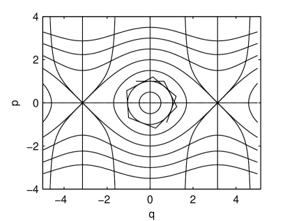
Figure 1: A DTH trajectory of a nonlinear pendulum. The v-shaped curves correspond to points where $\psi(z)=0$ and the horizontal and vertical lines correspond to points where $[\psi,\mathcal{H]}=0.$

Let $\psi_{k}=$ $\psi(z_{k}).$ We will show that, for points where $\psi_{k}\neq 0,$ the magnitude and sign of $\mathcal{H}_{k}/\psi_{k}$ is key to determining if a solution to the DTH equations exists and is locally unique. In particular, if $\mathcal{H}_{k}/\psi_{k}<0,$ and $\psi_{k}$ is sufficiently large, then no solution exists. If $\psi_{k}=0,$ the quantity $\mathcal{H}_{k}/\psi_{k}^{\prime},\$where $\psi^{\prime}=[\psi,\mathcal{H]},$ plays a similar role in determining existence and uniqueness. In the neighborhood of points where $\psi$ changes sign, a DTH trajectory bifurcates giving rise to “ghost trajectories”. Ghost trajectories are discussed in more detail in section 7.

The outline of this article is as follows. In section LABEL:decoupling_function, we use the Newton-Kantorovich Theorem to prove the existence and uniqueness of a function $\overline{z}(\lambda,z_{k})$ implicitly defined by equation (1a). We use the function $\overline{z}(\lambda,z_{k})$ to decouple equation (1b) from equation (1a). In section 4, we derive a cubic approximation of the Hamiltonian constraint function $g(\lambda,z_{k})=\mathcal{H(}\overline{z}(\lambda,z_{k})\mathcal{)}$. In section 5, we identify intervals where $g(\lambda,z_{k})$ is monotonic increasing/decreasing with respect to $\lambda$. Using monotonicity and the Intermediate Value Theorem, we prove the existence and uniqueness of Lagrange multipliers satisfying the decoupled, Hamiltonian constraint equation $g(\lambda,z_{k})=0$. The existence and uniqueness results for Lagrange multipliers is used in section 6 to prove the existence and uniqueness of DTH trajectories. SEM integration is shown, under certain conditions, to be well-posed. Finally, in section 7, we discuss ghost trajectories and the need to regularize the DTH equations of SEM integration.

3 Existence of a Decoupling Function

Consider the DTH equations (1a)–(1b). Equation (1a) can be rewritten as $f(\lambda,z_{k},\overline{z}_{k})=\overline{z}_{k}-z_{k}-\frac{1}{2}\lambda J\mathcal{H}_{z}\left(\overline{z}\right)=0$ where $\overline{z}_{k}=\frac{1}{2}(z_{k+1}+z_{k}).$ In Theorem 5 below, we prove that if the Hamiltonian function $\mathcal{H}(z)$ satisfies certain conditions, then there exists a smooth function $\overline{z}(\lambda,z_{k})$ such that $f(\lambda,z_{k},\overline{z}(\lambda,z_{k}))=0$ for all $\lambda\in[-\lambda_{\delta},\lambda_{\delta}]$ and $z_{k}\in U_{\delta}$ where $\lambda_{\delta}$ and $U_{\delta}$ are specified in Theorem 5. The function $\overline{z}(\lambda,z_{k})$ is used in section 5 to decouple equation (1b) from equation (1a). We begin by stating two standard results in numerical analysis, the Newton-Kantorovich Theorem [17] and the Matrix Perturbation Lemma [7].

Theorem 3 (Newton-Kantorovich Theorem)

Consider the function $f:U\rightarrow\mathcal{R}^{n}$ where $U\subset\mathcal{R}^{n}$ is open. Assume $f\in C^{1}(U)$ and $\left\|f_{x}(x_{2})-f_{x}(x_{1})\right\|\leq\gamma\left\|x_{2}-x_{1}\right\|$ for all $x_{1},x_{2}\in U.$ Assume there exists a point $x_{0}\in U$ and constants $\beta>0,$ $\eta>0$ such that $\left\|f_{x}(x_{0})^{-1}\right\|\leq\beta$ and $\left\|f_{x}(x_{0})^{-1}f(x_{0})\right\|\leq\eta$. Assume $\alpha<\frac{1}{2}$ where $\alpha=\beta\gamma\eta.$ Define $r_{-}=\left(1-\sqrt{1-2\alpha}\right)/\beta\gamma$ and $r_{+}=\left(1+\sqrt{1-2\alpha}\right)/\beta\gamma.$ If the close ball $\overline{B}(x_{0},r_{-})$ $\subset U,$ then the Newton iterates $x^{(i)},$ defined by $x^{(i+1)}=x^{(i)}-f_{x}(x^{(i)})^{-1}f(x^{(i)}),$ $i=0,1,\ldots,$ with $x^{(0)}=x_{0},$ are well defined and converge to $x_{\ast}\in\overline{B}(x_{0},r_{-})$ where $x_{\ast}$ is the unique solution of $f(x)=0$ in $\overline{B}(x_{0},r_{+})\cap U.$

Lemma 4 (Matrix Perturbation Lemma)

Assume the identity matrix $I$ is perturbed by the matrix $E.$ If $\left\|E\right\|\nolinebreak<\nolinebreak 1,$ then $\left(I-E\right)^{-1}$ exists, $\left(I-E\right)^{-1}=\sum_{n=0}^{\infty}E^{n}$ and $\left\|\left(I-E\right)^{-1}\right\|\nolinebreak<1\nolinebreak/\left(1-\left\|E\right\|\right).$

Theorem 5 (Decoupling Function)

Consider the extended-phase space Hamiltonian function $\mathcal{H}\in C^{2}(U)$ where $U\subset\mathcal{R}^{2n+2}$ is open. Assume $\left\|\mathcal{H}_{z}(z)\right\|\leq M_{1}$ and $\left\|\mathcal{H}_{zz}(z)\right\|\leq M_{2}$ for all $z\in U.$ Assume $\left\|\mathcal{H}_{zz}(z_{1})-\mathcal{H}_{zz}(z_{2})\right\|\leq\gamma_{H}\left\|z_{1}-z_{2}\right\|$ for all $z_{1,}z_{2}\in U.$ Let $\mathcal{\lambda}_{\delta}=\min(1/M_{2},1/\gamma_{H},\left(1-(1-\delta)^{2}\right)/2M_{1})$ and $U_{\delta}=\left\{z:\overline{B}(z,\delta)\subset U\right\}.$ Define $f(\lambda,z,\overline{z})=\overline{z}-z-\frac{1}{2}\lambda J\mathcal{H}_{z}\left(\overline{z}\right).$ Then, there exists a $\delta,$ where $0<\delta<1,$ and there exist a continuously differentiable function $\overline{z}:[-\mathcal{\lambda}_{\delta},\mathcal{\lambda}_{\delta}]\times U_{\delta}\rightarrow\mathcal{R}^{2n+2},$ such that $f(\lambda,z,\overline{z}(\lambda,z))=0\$for all $(\lambda,z)\in[-\mathcal{\lambda}_{\delta},\mathcal{\lambda}_{\delta}]\times U_{\delta}.$

Proof. First we show that for $\left|\lambda\right|\leq 1/M_{2},\$ $f_{\overline{z}}^{-1}$ exists and is bounded. Since $f_{\overline{z}}=I-E,$ where $E=$ $\frac{1}{2}\lambda J\mathcal{H}_{zz}$, and since $\left\|E\right\|\leq\frac{1}{2}\left(1/M_{2}\right)M_{2}=\frac{1}{2}<1,$ by the Matrix Perturbation Lemma, $f_{\overline{z}}^{-1}$ exists and $\left\|f_{\overline{z}}^{-1}\right\|<\beta,$ where $\beta=1/\left(1-\frac{1}{2}\right)=2.$ Next, we show that for $\left|\lambda\right|\leq 1/\gamma_{H}$, $f_{\overline{z}}$ is Lipschitz with respect to $\overline{z}$ with Lipschitz constant $\gamma=\frac{1}{2}$. We have

$$\left\|f_{\overline{z}}(\lambda,\overline{z}_{2},z)-f_{\overline{z}}(\lambda,\overline{z}_{1},z)\right\| =\left\|\frac{1}{2}\lambda J\mathcal{H}_{zz}(\overline{z}_{2})-\frac{1}{2}\lambda J\mathcal{H}_{zz}(\overline{z}_{1})\right\|$$

$$\leq\frac{1}{2}\frac{1}{\gamma_{H}}\gamma_{H}\left\|\overline{z}_{2}-\overline{z}_{1}\right\|$$

$$=\frac{1}{2}\left\|\overline{z}_{2}-\overline{z}_{1}\right\|.$$

Now consider using Newton’s iteration to solve $f(\lambda,z_{k},\overline{z})=0$ for $\overline{z}.$ If we initialize the iteration with $\overline{z}^{(0)}=z_{k},$ we have $\eta=\left\|f_{\overline{z}}^{-1}(\lambda,z_{k},z_{k})f(\lambda,z_{k},z_{k})\right\|\leq\left\|f_{\overline{z}}^{-1}\right\|\left\|\frac{1}{2}\lambda J\mathcal{H}_{z}\right\|.$ Let $\mathcal{\lambda}_{\delta}=\min(1/M_{2},1/\gamma_{H},\left(1-(1-\delta)^{2}\right)/2M_{1}).$ For $\left|\lambda\right|\leq\mathcal{\lambda}_{\delta},$ it follows that $\eta<2\frac{1}{2}\left(1-(1-\delta)^{2}\right)/\left(2M_{1}\right)M_{1}=\left(1-(1-\delta)^{2}\right)/2.$ For $0<\delta<1,$ we have then that $\ \alpha=\beta\gamma\eta<2\frac{1}{2}\left(1-(1-\delta)^{2}\right)/2<\frac{1}{2}.$ Therefore,

$$r_{-}=\frac{1-\sqrt{1-2\alpha}}{\beta\gamma}<\frac{1-\sqrt{1-2\left(\frac{1-(1-\delta)^{2}}{2}\right)}}{2\frac{1}{2}}=\delta.$$

It follows that for $z_{k}\in U_{\delta},$ $\overline{B}(z_{k},r_{-})\subset\overline{B}(z_{k},\delta)\subset U.$ By the Newton-Kantorovich Theorem, the function $\overline{z}(\lambda,z_{k})$ is well defined on $[-\mathcal{\lambda}_{\delta},\mathcal{\lambda}_{\delta}]\times U_{\delta}$ and $f(\lambda,z_{k},\overline{z}(\lambda,z_{k}))\equiv 0.$ (We assume $\delta$ is chosen small enough that $U_{\delta}$ is nonempty.) The Implicit Function Theorem implies $\overline{z}(\lambda,z_{k})$ is continuously differentiable.   

4 Cubic Approximation of the Hamiltonian Constraint

Given $\lambda_{k}\in[-\mathcal{\lambda}_{\delta},\mathcal{\lambda}_{\delta}]$ and $z_{k}\in U_{\delta},$ Theorem 5 implies there exists a point $\overline{z}_{k}=$ $\overline{z}(\lambda_{k},z_{k})$ and a point $z_{k+1}=2\overline{z}_{k}-$ $z_{k},\$such that $\lambda_{k},$ $z_{k}$ and $z_{k+1}$ satisfy the first DTH equation, $\Delta z_{k}=\lambda_{k}J\mathcal{H}_{z}(\overline{z}_{k})\ .$ We use $\overline{z}(\lambda,z_{k})$ to decouple the second DTH equation, $\mathcal{H}(\overline{z}_{k})=0,$ from the first DTH equation by defining the function $g(\lambda,z_{k})=\mathcal{H}(\overline{z}(\lambda,z_{k}))$ and replacing the second equation with the equation $g(\lambda,z_{k})=0.$

In this section, we determine a cubic approximation of $g(\lambda,z_{k})$ as a function of $\lambda.$ Obtaining this approximation is made difficult by the fact that the function $\overline{z}(\lambda,z_{k})$ is only implicitly defined. We will see that the linear term in the cubic approximation of $g(\lambda,z_{k})$ is always equal to zero. The analysis of DTH dynamics is also complicated by this fact since we are forced to consider the effects of the quadratic and even cubic term in the cubic approximation of $g(\lambda,z_{k}).$

The outline of this section is as follows. In Lemma 6 below, we show that $\overline{z}_{\lambda}(\lambda,z_{k})$ is Lipschitz continuous with respect to $\lambda.$ In Lemma 7 we define the important function $\psi(z)=\left(J\mathcal{H}_{z}\right)^{\top}\mathcal{H}_{zz}\left(J\mathcal{H}_{z}\right)\$and we approximate the partial derivative $\partial g(\lambda,z_{k})/\partial\lambda$ by the simpler function $-\frac{1}{4}\lambda\,h(\lambda,z_{k})$ where $h(\lambda,z_{k})=$ $\psi\mathcal{(}\overline{z}(\lambda,z_{k})).$ In Lemma 8, we prove that $\partial h(\lambda,z_{k})/\partial\lambda$ is Lipschitz continuous with respect to $\lambda.$ Finally, in Lemma 9, we determine a cubic approximate of $g(\lambda,z_{k}).$

Lemma 6

For $\lambda_{1},\lambda_{2}\in[-\mathcal{\lambda}_{\delta},\mathcal{\lambda}_{\delta}]$ and $z_{k}\in U_{\delta},$

$$\left\|\overline{z}_{\lambda}(\lambda_{2},z_{k})-\overline{z}_{\lambda}(\lambda_{1},z_{k})\right\|\leq\gamma_{z}\left|\lambda_{2}-\lambda_{1}\right|\text{ }$$

where $\gamma_{z}=2M_{1}M_{2}+\,M_{1}^{2}.$

The proof is given in the appendix.

Lemma 7

Define the functions $g(\lambda,z_{k})=\mathcal{H(}\overline{z}(\lambda,z_{k})),$ $\psi(z)=\left(J\mathcal{H}_{z}\right)^{\top}\mathcal{H}_{zz}\left(J\mathcal{H}_{z}\right)\$and $h(\lambda,z_{k})=\psi\mathcal{(}\overline{z}(\lambda,z_{k})).$ Then, for $\left|\lambda\right|\leq\lambda_{\delta}\$and $z_{k}\in U_{\delta},$

$$\left|\frac{\partial g(\lambda,z_{k})}{\partial\lambda}-\left(-\frac{1}{4}\lambda h(\lambda,z_{k})\right)\right|\leq\frac{1}{8}M_{1}^{2}M_{2}^{3}\left|\lambda\right|^{3}\text{ }.$$

Proof. Since $f_{\overline{z}}^{-1}=\left(I-E\right)^{-1}$ where $E=$ $\frac{1}{2}\lambda J\mathcal{H}_{zz},$ for $\left|\lambda\right|\leq\lambda_{\delta}\$we have$\ \left\|E\right\|\leq\frac{1}{2}<1.$ By the Matrix Perturbation Lemma we have

$$f_{\overline{z}}^{-1} =I+E+E^{2}+E^{3}+E^{4}+\cdots$$

$$=I+E+E^{2}+E^{3}(I+E+\cdots)$$

$$=I+E+E^{2}+E^{3}f_{\overline{z}}^{-1}.$$

Therefore,

$$\frac{\partial g(\lambda,z_{k})}{\partial\lambda} =\mathcal{H}_{z}^{\top}\overline{z}_{\lambda}$$

$$=\frac{1}{2}\mathcal{H}_{z}^{\top}\left(f_{\overline{z}}^{-1}J\right)\mathcal{H}_{z}$$

$$=\frac{1}{2}\left(\mathcal{H}_{z}^{\top}J\mathcal{H}_{z}+\mathcal{H}_{z}^{\top}\left(EJ\right)\mathcal{H}_{z}\right.$$

$$+\left.\mathcal{H}_{z}^{\top}\left(E^{2}J\right)\mathcal{H}_{z}+\mathcal{H}_{z}^{\top}\left(E^{3}f_{\overline{z}}^{-1}J\right)\mathcal{H}_{z}\right).$$ (3)

Since both $J$ and $E^{2}J=\frac{1}{4}\lambda^{2}\left(J\mathcal{H}_{zz}J\mathcal{H}_{zz}J\right)$ are skew-symmetric, the first and third term in (3) equal zero. The second term is given by

$$\mathcal{H}_{z}^{\top}\left(EJ\right)\mathcal{H}_{z} =-\frac{1}{2}\lambda\left(J\mathcal{H}_{z}\right)^{\top}\mathcal{H}_{zz}\left(J\mathcal{H}_{z}\right)$$

$$=-\frac{1}{2}\lambda\psi(\overline{z}(\lambda,z_{k}))$$

$$=-\frac{1}{2}\lambda h(\lambda,z_{k}).$$ (4)

Thus, equations (3) and (4) imply

$$\left|\frac{\partial g(\lambda,z_{k})}{\partial\lambda}-\left(-\frac{1}{4}\lambda h(\lambda,z_{k})\right)\right| =\left|\frac{1}{2}\mathcal{H}_{z}^{\top}\left(E^{3}f_{\overline{z}}^{-1}J\right)\mathcal{H}_{z}\right|$$

$$\leq\frac{1}{8}M_{1}^{2}M_{2}^{3}\left|\lambda\right|^{3}.$$

 

Lemma 8

Assume $\psi\in C^{2}(U)$, $\left\|\psi_{z}(z)\right\|\leq N_{1}$ and $\left\|\psi_{zz}(z)\right\|\leq N_{2}$ for $z\in U.$ Then, for $\lambda_{1},\lambda_{2}\in[-\mathcal{\lambda}_{\delta},\mathcal{\lambda}_{\delta}]$ and $z_{k}\in U_{\delta},$

$$\left|\frac{\partial h(\lambda_{2},z_{k})}{\partial\lambda}-\frac{\partial h(\lambda_{1},z_{k})}{\partial\lambda}\right|\leq\gamma_{h}\left|\lambda_{2}-\lambda_{1}\right|\$$

where $\gamma_{h}=N_{1}\gamma_{z}+M_{1}^{2}N_{2}.$

The proof is given in the appendix.

Lemma 9

Assume $\psi\in C^{2}(U)$, $\left\|\psi_{z}(z)\right\|\leq N_{1}$ and $\left\|\psi_{zz}(z)\right\|\leq N_{2}$ for $z\in U.$ Let $\mathcal{H}_{k}=\mathcal{H}(z_{k}),$ $\psi_{k}=\psi(z_{k})$ and $\psi_{k}^{\prime}=\left.[\psi,\mathcal{H}]\right|_{z=z_{k}}.$ Then, for $\left|\lambda\right|\leq\lambda_{\delta}$ and $z_{k}\in U_{\delta},$

$$\left|\frac{\partial g(\lambda,z_{k})}{\partial\lambda}-\left(-\frac{1}{4}\psi_{k}\lambda-\frac{1}{8}\psi_{k}^{\prime}\,\lambda^{2}\right)\right|\leq 4K\left|\lambda\right|^{3}$$ (5)

and

$$\left|g(\lambda,z_{k})-\left(\mathcal{H}_{k}-\frac{1}{8}\psi_{k}\lambda^{2}-\frac{1}{24}\psi_{k}^{\prime}\lambda^{3}\right)\right|\leq K\left|\lambda\right|^{4}$$ (6)

where $K=\frac{1}{32}(M_{1}^{2}M_{2}^{3}+2\gamma_{h})$.

Proof. The Mean Value Theorem implies there exists a $\widetilde{\lambda}$ between $0$ and $\lambda$ such that $h(\lambda,z_{k})-h(0,z_{k})=\left(\partial h(\widetilde{\lambda},z_{k})/\partial\lambda\right)\lambda.$ Therefore, using Lemma 8,

$$\left|h(\lambda,z_{k})-h(0,z_{k})-\frac{\partial h}{\partial\lambda}(0,z_{k})\,\lambda\right| =\left|\frac{\partial h}{\partial\lambda}(\widetilde{\lambda},z_{k})\,\lambda-\frac{\partial h}{\partial\lambda}(0,z_{k})\,\lambda\right|$$

$$\leq\gamma_{h}|\widetilde{\lambda|}\left|\lambda\right|\leq\gamma_{h}\left|\lambda\right|^{2}.$$

Since $h(0,z_{k})=\psi_{k}$ and $\partial h(0,z_{k})/\partial\lambda=\frac{1}{2}\psi_{k}^{\prime},\$we have $\left|h(\lambda,z_{k})-\psi_{k}-\frac{1}{2}\psi_{k}^{\prime}\,\lambda\right|\leq\gamma_{h}\left|\lambda\right|^{2}.$ Using Lemma 7, we establish inequality (5) as follows.

$$\left|\frac{\partial g(\lambda,z_{k})}{\partial\lambda}-\left(-\frac{1}{4}\psi_{k}\lambda-\frac{1}{8}\psi_{k}^{\prime}\,\lambda^{2}\right)\right| \leq\left|\frac{\partial g(\lambda,z_{k})}{\partial\lambda}-\left(-\frac{1}{4}\lambda h(\lambda,z_{k})\right)\right|$$

$$+\left|\left(-\frac{1}{4}\lambda h(\lambda,z_{k})\right)-\left(-\frac{1}{4}\psi_{k}\lambda-\frac{1}{8}\psi_{k}^{\prime}\,\lambda^{2}\right)\right|$$

$$\leq 4K\left|\lambda\right|^{3}\$$ (7)

where $K=\frac{1}{32}(M_{1}^{2}M_{2}^{3}+2\gamma_{h})$. We establish (6) as follows. First, using (7) we have

$$\left|{\displaystyle\int_{0}^{\lambda}}\left(\frac{\partial g(\lambda,z_{k})}{\partial\lambda}+\frac{1}{4}\psi_{k}\lambda+\frac{1}{8}\psi_{k}^{\prime}\,\lambda^{2}\right)\,d\lambda\right| \leq{\displaystyle\int_{0}^{\lambda}}\left|\frac{\partial g(\lambda,z_{k})}{\partial\lambda}+\frac{1}{4}\psi_{k}\lambda+\frac{1}{8}\psi_{k}^{\prime}\,\lambda^{2}\right|\,d\lambda$$

$$\leq 4K{\displaystyle\int_{0}^{\lambda}}\left|\lambda\right|^{3}\,d\lambda$$

$$=K\left|\lambda\right|^{4}.$$

But

$${\displaystyle\int_{0}^{\lambda}}\left(\dfrac{\partial g(\lambda,z_{k})}{\partial\lambda}+\dfrac{1}{4}\psi_{k}\lambda+\dfrac{1}{8}\psi_{k}^{\prime}\,\lambda^{2}\right)\,d\lambda=g(\lambda,z_{k})-g(0,z_{k})+\dfrac{1}{8}\psi_{k}\lambda^{2}+\dfrac{1}{24}\psi_{k}^{\prime}\,\lambda^{3}.$$

So we have

$$\left|g(\lambda,z_{k})-\left(\mathcal{H}_{k}-\frac{1}{8}\psi_{k}\lambda^{2}-\frac{1}{24}\psi_{k}^{\prime}\lambda^{3}\right)\right|\leq K\left|\lambda\right|^{4}.$$

 

5 Existence and Uniqueness of Lagrange Multipliers

In this section, we address the question of the existence and uniqueness of Lagrange multipliers $\lambda$ which satisfy the decoupled, Hamiltonian constraint equation $g(\lambda,z_{k})=0.$ We begin by proving a monotonicity result for the function $g(\lambda,z_{k}).$ Then we prove three separate existence and uniqueness theorems, Theorems 11–13, each of which accounts for one of the three regions of extended-phase space described below. (The value of the constant $K$ is determined by the Hamiltonian function $\mathcal{H}(z).$ See Lemma 9.)

region I $$\left\{z_{k}:\psi(z_{k})\neq 0,\ (\psi^{\prime}(z_{k}))^{2}\leq 24K\left|\psi(z_{k})\right|\right\}$$

region II

region III

    

The proofs of each of the three existence and uniqueness theorems in this section uses the same basic approach. First, we derive bounds for the function $g(\lambda,z_{k})/\psi(z_{k}).$ (See Figure 2.) Then, we use monotonicity and the Intermediate Value Theorem to establish the existence and (local) uniqueness of Lagrange multipliers $\lambda$ satisfying the equation $g(\lambda,z_{k})=0$.

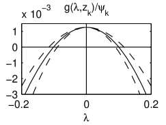
(a) region I

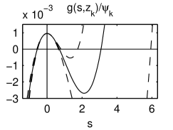
(b) region II

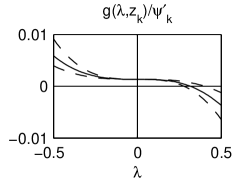
(c) region III

Figure 2: Bounds on $g(\lambda,z_{k})/\psi(z_{k})$ for the nonlinear pendulum.

Lemma 10 (Monotonicity)

Assume $z_{k}\in U_{\delta}.$ Then we claim the following:

1. If $\psi_{k}\neq 0,$ $(\psi_{k}^{\prime})^{2}\leq 24K\left|\psi_{k}\right|$ and $\left|\lambda\right|\leq\Lambda_{k}$ where $0<\Lambda_{k}<\min(\sqrt{\left|\psi_{k}\right|/96K},\lambda_{\delta}),$ then $g(\lambda,z_{k})$ is monotonic increasing/decreasing in the intervals $(-\Lambda_{k},0)$ and $(0,\Lambda_{k}).$

2. Assume $\psi_{k}\neq 0,$ $(\psi_{k}^{\prime})^{2}>24K\left|\psi_{k}\right|$ and $\left|\lambda\right|\leq\Lambda_{k}$ where $0<\Lambda_{k}<\min(\left|\psi_{k}^{\prime}\right|/48K,\lambda_{\delta}).$ Let $g(s,z_{k})$ be a reparametrization of $g(\lambda,z_{k})$ where $s=-(\psi_{k}^{\prime}/\psi_{k})\lambda.$ Define $S_{k}=\left|\psi_{k}^{\prime}/\psi_{k}\right|\Lambda_{k}$. Then $g(s\,,z_{k})$ is monotonic increasing/decreasing in the following intervals: a) $(-S_{k},0)$, b) $(0,S_{k})$ if $S_{k}<\frac{6}{5},$ c) $(0,\frac{6}{5})$ if $S_{k}\geq\frac{6}{5}$ and d) $(6,S_{k})$ if $S_{k}>6.$

3. If $\psi_{k}=0,$ $\psi_{k}^{\prime}\neq 0,$ and $\left|\lambda\right|\leq\Lambda_{k}$ where $0<\Lambda_{k}<\min(\left|\psi_{k}^{\prime}\right|/48K,\lambda_{\delta}),$ then $g(\lambda,z_{k})$ is monotonic increasing/decreasing in the intervals $(-\Lambda_{k},0)$ and $(0,\Lambda_{k}).$

The proof of Lemma 10 is given in the appendix.

Theorem 11 below deals with region I of extended-phase space where the quadratic term dominates the cubic term in the cubic approximation of $g(\lambda,z_{k}).$ See Figure 3 for plots of $g(\lambda,z_{k})/\psi_{k}$ in region I of the nonlinear pendulum. Since $g(0,z_{k})=\mathcal{H(}\overline{z}(0,z_{k}))=\mathcal{H}(z_{k})\mathcal{=H}_{k},$ we see from Figure 3 that the sign of $\mathcal{H}_{k}/\psi_{k}$ determines the number of solutions to the equation $g(\lambda,z_{k})=0.$

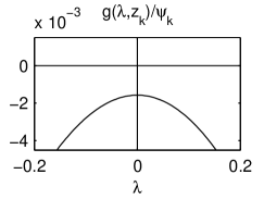
(a) $\mathcal{H}_{k}/\psi_{k}<0$

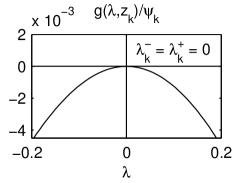
(b) $\mathcal{H}_{k}/\psi_{k}=0$

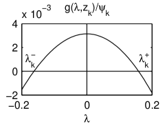
(c) $\mathcal{H}_{k}/\psi_{k}>0$

Figure 3: Plots of $g(\lambda,z_{k})/\psi(z_{k})$ in region I of the nonlinear pendulum.

Theorem 11

Assume $z_{k}\in U_{\delta},$ $\psi_{k}\neq 0$, $(\psi_{k}^{\prime})^{2}\leq 24K\left|\psi_{k}\right|\$and $\left|\lambda\right|<\Lambda_{k}$ where $0<\Lambda_{k}<\min(\sqrt{\left|\psi_{k}\right|/96K},\lambda_{\delta}).$ Then the following statements about the equation $g(\lambda,z_{k})=0$ are true.

1. If $\mathcal{H}_{k}/\psi_{k}<0,$ no solution exists.

2. If $\mathcal{H}_{k}/\psi_{k}=0,$ the only solution is $\lambda=0$.

3. If $0<\mathcal{H}_{k}/\psi_{k}<\frac{3}{32}\Lambda_{k}^{2},$ two solutions of opposite sign exist, $\lambda_{k}^{-}\in(-\Lambda_{k},0)$ and $\lambda_{k}^{+}\in(0,\Lambda_{k})$. The solutions are unique within their respective intervals.

4. If $\mathcal{H}_{k}/\psi_{k}>\frac{5}{32}\Lambda_{k}^{2},$ no solution exists.

Proof. Since $\left|\lambda\right|\leq\Lambda_{k}<\sqrt{\left|\psi_{k}\right|/96K},$ we have from inequality (6) of Lemma 9 that

$$\left|\frac{g(\lambda,z_{k})}{\psi_{k}}-\left(\dfrac{\mathcal{H}_{k}}{\psi_{k}}-\frac{1}{8}\lambda^{2}-\frac{1}{24}\dfrac{\psi_{k}^{\prime}}{\psi_{k}}\lambda^{3}\right)\right|\leq\frac{K}{\left|\psi_{k}\right|}\left|\lambda\right|^{4}\leq\frac{1}{96}\lambda^{2}.$$

It follows that

$$\dfrac{\mathcal{H}_{k}}{\psi_{k}}-\frac{13}{96}\lambda^{2}-\frac{1}{24}\left|\dfrac{\psi_{k}^{\prime}}{\psi_{k}}\lambda\right|\lambda^{2}\leq\frac{g(\lambda,z_{k})}{\psi_{k}}\leq\dfrac{\mathcal{H}_{k}}{\psi_{k}}-\frac{11}{96}\lambda^{2}+\frac{1}{24}\left|\dfrac{\psi_{k}^{\prime}}{\psi_{k}}\lambda\right|\lambda^{2}.$$ (8)

Since by assumption $(\psi_{k}^{\prime})^{2}\leq 24K\left|\psi_{k}\right|,$ we have

$$\left|\frac{\psi_{k}^{\prime}}{\psi_{k}}\lambda\right|=\left|\frac{\psi_{k}^{\prime}}{\psi_{k}}\right|\left|\lambda\right|<\frac{\sqrt{24K\left|\psi_{k}\right|}}{\left|\psi_{k}\right|}\sqrt{\frac{\left|\psi_{k}\right|}{96K}}=\frac{1}{2}.$$ (9)

Using (8) and (9) we have

$$\dfrac{\mathcal{H}_{k}}{\psi_{k}}-\frac{5}{32}\lambda^{2}\leq\frac{g(\lambda,z_{k})}{\psi_{k}}\leq\dfrac{\mathcal{H}_{k}}{\psi_{k}}-\frac{3}{32}\lambda^{2}.$$ (10)

To establish (i), assume $\mathcal{H}_{k}/\psi_{k}<0.$ Then inequality (10) implies $g(\lambda,z_{k})/\psi_{k}<0$ for all $\left|\lambda\right|\leq\Lambda_{k}$ and no solution exists. If $\mathcal{H}_{k}/\psi_{k}=0,$ then $g(\lambda,z_{k})/\psi_{k}<0$ for nonzero $\lambda.$ Since $g(0,z_{k})=\mathcal{H}_{k}=0,$ the only solution is $\lambda=0,$ establishing (ii). If we assume $0<\mathcal{H}_{k}/\psi_{k}<\frac{3}{32}\Lambda_{k}^{2},$ then $g(\pm\Lambda_{k},z_{k})/\psi_{k}\leq\mathcal{H}_{k}/\psi_{k}-\frac{3}{32}\Lambda_{k}^{2}<0.$ Since $g(0,z_{k})/\psi_{k}=\mathcal{H}_{k}/\psi_{k}>0,$ the Intermediate Value Theorem implies $g(\lambda,z_{k})=0$ has two solutions $\lambda_{k}^{-}\in(-\Lambda_{k},0)$ and $\lambda_{k}^{+}\in(0,\Lambda_{k}).$ Lemma 10(i) implies $g(\lambda,z_{k})$ is monotonic in each interval establishing uniqueness and claim (iii). Finally, if $\mathcal{H}_{k}/\psi_{k}>\frac{5}{32}\Lambda_{k}^{2},$ then inequality (10) implies that for all $\left|\lambda\right|\leq\Lambda_{k},$

$$0<\frac{\mathcal{H}_{k}}{\psi_{k}}-\frac{5}{32}\Lambda_{k}^{2}\leq\frac{\mathcal{H}_{k}}{\psi_{k}}-\frac{5}{32}\lambda^{2}\leq\frac{g(\lambda,z_{k})}{\psi_{k}}$$

establishing claim (iv).   

Theorem 12 below deals with region II of extended-phase space where $\psi(z)$ is small but nonzero. Theorem 12 is the most complex of the three existence and uniqueness theorems in this section because both quadratic and cubic terms need to be taken into consideration. The reparametrization $s=-\left(\psi_{k}^{\prime}/\psi_{k}\right)\lambda$ simplifies the statement of the theorem and its proof. See Figure 4 for plots of $g(\lambda,z_{k})/\psi_{k}$ in region II of the nonlinear pendulum. We can see from Figure 4 that the sign of $\mathcal{H}_{k}/\psi_{k}$ determines the number of solutions to the equation $g(s,z_{k})=0.$ (Recall that $g(0,z_{k})=\mathcal{H}_{k}.$) Note the appearance of a “ghost solution”, $s_{k}^{\ast}$. From Figure 4(c), we see that, unlike the two solutions $s_{k}^{-}$ and $s_{k}^{+},$ the ghost solution $s_{k}^{\ast}$ does not approach zero as $\mathcal{H}_{k}/\psi_{k}\rightarrow 0^{+}.$

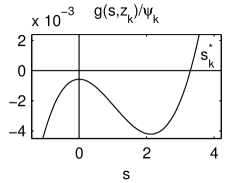
(a) $\mathcal{H}_{k}/\psi_{k}<0$

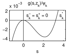
(b) $\mathcal{H}_{k}/\psi_{k}=0$

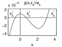
(c) $\mathcal{H}_{k}/\psi_{k}>0$

Figure 4: Plots of $g(\lambda,z_{k})/\psi(z_{k})$ in region II of the nonlinear pendulum.

Theorem 12

Assume $z_{k}\in U_{\delta},$ $\psi_{k}\neq 0$, $(\psi_{k}^{\prime})^{2}>24K\left|\psi_{k}\right|\$and $\left|\lambda\right|<\Lambda_{k}$ where $0<\Lambda_{k}<\min(\left|\psi_{k}^{\prime}\right|/48K,\lambda_{\delta}).$ Let $g(s,z_{k})$ be a reparametrization of $g(\lambda,z_{k})$ where $s=-\left(\psi_{k}^{\prime}/\psi_{k}\right)\lambda$. Define $S_{k}=$ $\left|\psi_{k}^{\prime}/\psi_{k}\right|\Lambda_{k}.$ Then the following statements about the equation $g(s,z_{k})=0$ are true.

1. If $\mathcal{H}_{k}/\psi_{k}<0,$ no solution exists in the interval $(-S_{k},2).$

2. If $\mathcal{H}_{k}/\psi_{k}=0,$ the only solution in the interval $(-S_{k},2)$ is $s=0.$

3. If $\tfrac{1}{48}\Lambda_{k}^{2}(6-S_{k})<\mathcal{H}_{k}/\psi_{k}\leq 0$ for $S_{k}>6,$ there exists a solution $s_{k}^{\ast}\in[2,S_{k}).$

4. If $0<\mathcal{H}_{k}/\psi_{k}<\tfrac{1}{48}\Lambda_{k}^{2}(6+S_{k}),$ there exists a solution $s_{k}^{-}\in(-S_{k},0)\$and the solution is unique in this interval.

5. If $0<\mathcal{H}_{k}/\psi_{k}<\tfrac{1}{16}\Lambda_{k}^{2}(2-S_{k})$ for $S_{k}<\frac{6}{5},$ there exists a solution $s_{k}^{+}\in(0,S_{k})$ and the solution is unique in this interval.

6. If $0\leq\mathcal{H}_{k}/\psi_{k}<\frac{9}{125}\left(\psi_{k}/\psi_{k}^{\prime}\right)^{2}$ and

   1. if $S_{k}\geq\frac{6}{5},$ there exists a solution $s_{k}^{+}\in[0,\frac{6}{5})$ and the solution is unique in this interval.

   2. if $S_{k}\geq 6,$ there exists a solution $s_{k}^{\ast}\in(\frac{6}{5},S_{k}).$

7. If $\mathcal{H}_{k}/\psi_{k}>\frac{2}{3}\left(\psi_{k}/\psi_{k}^{\prime}\right)^{2},$ no solution exists in $(0,S_{k}).$

The proof of Theorem 12 is given in the appendix.

Theorem 13 below deals with region III of extended-phase space where the quadratic term of the cubic approximation of $g(\lambda,z_{k})$ is equal to zero. See Figure 5 for plots of $g(\lambda,z_{k})/\psi_{k}^{\prime}$ in region III of the nonlinear pendulum. As we can see from Figure 5, the sign of $\mathcal{H}_{k}/\psi_{k}^{\prime}$ determines whether the solution $\lambda_{k}^{-}$ or $\lambda_{k}^{+}$ exists.

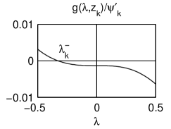
(a) $\mathcal{H}_{k}/\psi^{\prime}_{k}<0$

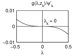
(b) $\mathcal{H}_{k}/\psi^{\prime}_{k}=0$

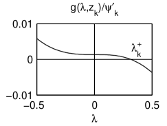
(c) $\mathcal{H}_{k}/\psi^{\prime}_{k}>0$

Figure 5: Plots of $g(\lambda,z_{k})/\psi\prime(z_{k})$ in region III of the nonlinear pendulum.

Theorem 13

Assume $z_{k}\in U_{\delta},$ $\psi_{k}=0$, $\psi_{k}^{\prime}\neq 0\$and $\left|\lambda\right|\leq\Lambda_{k}$ where $0<\Lambda_{k}<\min(\left|\psi_{k}^{\prime}\right|/48K,\lambda_{\delta}).$ Then the following statements about the equation $g(\lambda,z_{k})=0$ are true.

1. If $-\tfrac{1}{48}\Lambda_{k}^{3}<\mathcal{H}_{k}/\psi_{k}^{\prime}<0,$ there exists a solution $\lambda_{k}^{-}\in(-\Lambda_{k},0)$ and it is unique in this interval. No solution exists in $[0,\Lambda_{k}).$

2. If $0<\mathcal{H}_{k}/\psi_{k}^{\prime}<\tfrac{1}{48}\Lambda_{k}^{3},$ there exists a solution $\lambda_{k}^{+}\in(0,\Lambda_{k})$ and it is unique in this interval. No solution exists in $(-\Lambda_{k},0].$

3. If $\mathcal{H}_{k}/\psi_{k}^{\prime}=0,$ the only solution is $\lambda=0.$

4. If $\left|\mathcal{H}_{k}/\psi_{k}^{\prime}\right|>\tfrac{1}{16}\Lambda_{k}^{3},$ no solution exists.

The proof of Theorem 13 is given in the appendix.

6 Existence and Uniqueness of DTH Trajectories

The main result of this article is stated below in Theorem 14. The proof of Theorem 14 uses Theorems 11–13 from the previous section. Before stating the theorem, we provide a condensed description of the theorem’s main conclusions.

Consider a point $z_{0}$ in extended-phase space. Roughly speaking, when $\left|\mathcal{H}_{0}/\psi_{0}\right|$ is sufficiently small, there are four generic possibilities for DTH trajectories. (1) If $\mathcal{H}_{0}/\psi_{0}\geq 0$ and $\left|\psi_{0}\right|$ is large, then a unique DTH trajectory exists which passes through the vertex point $z_{0.}$ (2) If $\mathcal{H}_{0}/\psi_{0}\geq 0$ and $\psi$ changes sign near $z_{0}$, then a DTH trajectory exists which bifurcates at the vertex point $z_{0.}$ (3) If $\mathcal{H}_{0}/\psi_{0}<0$ and $\psi$ changes sign near $z_{0}$, then a DTH trajectory exists which either begins or ends at the vertex point $z_{0}.$ (4) If $\mathcal{H}_{0}/\psi_{0}<0$ and $\left|\psi_{0}\right|$ is large, then no DTH trajectory can exist having $z_{0}$ as a vertex point. See Figure 6 for plots of DTH trajectories of the nonlinear pendulum for the following initial conditions: (a) $z_{0}=(-0.15,-0.05,0,-3.48)$ (b) $z_{0}=(1.25,-0.05,0,-4.33)$ (c) $z_{0}=(1.85,-0.05,0,-4.87)$.

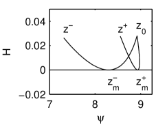
(a) passing through $z_{0}$.

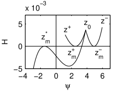
(b) bifurcating at $z_{0}$.

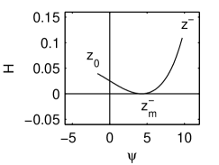
(c) terminating at $z_{0}$.

Figure 6: DTH trajectories of the nonlinear pendulum.

Since DTH trajectories preserve the symplectic-energy-momentum properties of Hamiltonian dynamics, Theorem 14 provides conditions under which a SEM integrator is well-posed. As a practical matter, we point out that, for classical Hamiltonians, generic possibility (4), where no DTH trajectory exists, can always be avoided by choosing an initial value for $\wp_{0}\$(the momentum conjugate to time) which is sufficiently small and of the appropriate sign. Generic possibilities (2) and (3) are more challenging to deal with and are discussed further in section 7.

Theorem 14 (Existence & Uniqueness of DTH Trajectories)

Consider an extended-phase space Hamiltonian function $\mathcal{H}\in C^{2}(U)$ where $U\subset\Re^{2n+2}$ is open. Define $\psi(z)=\left(J\mathcal{H}_{z}\right)^{\top}\mathcal{H}_{zz}\left(J\mathcal{H}_{z}\right)$ and $\psi^{\prime}(z)=[\psi,\mathcal{H]}.$ Assume $\mathcal{H}_{z},$ $\mathcal{H}_{zz},$ $\psi_{z}$ and $\psi_{zz}$ are bounded on $U$ and $\mathcal{H}_{zz}$ is Lipschitz continuous on $U.$ Assume also that $z_{k}\in U_{\delta}\$where $U_{\delta}\ =\left\{z:\overline{B}(z,\delta)\subset U\right\}$ and $0<\delta<1$. If $\psi_{k}\neq 0,$ then there exists a $\Lambda_{k}>0$ for which statements (i)–(iii) are true.

1. If $\mathcal{H}_{k}/\psi_{k}<0$, then $z_{k}$ can not be a vertex point or end point of a DTH trajectory with Lagrange multiplier(s) $\left|\lambda\right|\leq\Lambda_{k}$.

2. If $\mathcal{H}_{k}/\psi_{k}=0,$ then $z_{k}$ is a vertex point of a fixed-point DTH trajectory with Lagrange multiplier $\lambda_{k}=0.$ No other DTH trajectory with Lagrange multiplier(s) $\left|\lambda_{k}\right|\leq\Lambda_{k}$ exists.

3. If $\mathcal{H}_{k}/\psi_{k}>0$ is sufficiently small, then $z_{k}$ is a vertex point of a unique DTH trajectory passing through $z_{k}$ with Lagrange multipliers $\left|\lambda_{k}^{\pm}\right|\leq\Lambda_{k}.$

If $\left|\psi_{k}\right|\neq 0$ is sufficiently small and $\psi_{k}^{\prime}\neq 0,$ then there exists a $\Lambda_{k}>0$ for which statements (iv)–(vi) are true.

1. If $\mathcal{H}_{k}/\psi_{k}<0$ and $\left|\mathcal{H}_{k}/\psi_{k}\right|$ is sufficiently small, then $z_{k}$ is a vertex point of a DTH trajectory which begins (ends) at $z_{k}$ and has Lagrange multiplier $\left|\lambda_{k}^{\ast}\right|\leq\Lambda_{k}.$

2. If $\mathcal{H}_{k}/\psi_{k}=0,$ then a DTH trajectory exists which bifurcates at $z_{k}$ into a, fixed point, DTH trajectory with Lagrange multiplier $\lambda_{k}=0$ and a ghost DTH trajectory with Lagrange multiplier $\left|\lambda_{k}^{\ast}\right|\leq\Lambda_{k}.$

3. If $\mathcal{H}_{k}/\psi_{k}>0$ is sufficiently small, then a DTH trajectory exists which bifurcates at $z_{k}$ into a DTH trajectory with Lagrange multipliers $\left|\lambda_{k}^{\pm}\right|\leq\Lambda_{k}$ and a ghost DTH trajectory with Lagrange multiplier $\left|\lambda_{k}^{\ast}\right|\leq\Lambda_{k}.$

If $\psi_{k}=0$ and $\psi_{k}^{\prime}\neq 0$, then there exists a $\Lambda_{k}>0$ for which statements (vii) and (viii) are true.

1. If $\left|\mathcal{H}_{k}/\psi_{k}^{\prime}\right|\neq 0$ is sufficiently small, then $z_{k}$ is a vertex point of a unique DTH trajectory which begins (ends) at $z_{k}$ with Lagrange multiplier $\left|\lambda_{k}\right|\leq\Lambda_{k}.$

2. If $\mathcal{H}_{k}/\psi_{k}^{\prime}=0,$ then $z_{k}$ is a vertex point of a fixed-point DTH trajectory with Lagrange multiplier $\lambda_{k}=0.$ No other DTH trajectory with Lagrange multiplier $\left|\lambda_{k}\right|\leq\Lambda_{k}$ exists.

Proof. Consider the DTH equations

$$\Delta z_{k} =\lambda J\mathcal{H}_{z}(\overline{z})$$ (11)

$$\mathcal{H}(\overline{z}) =0$$ (12)

where $\Delta z_{k}=z-z_{k},$ $\overline{z}=\frac{1}{2}(z+z_{k})$ and $\mathcal{H\in}C^{2}(U).$ We can rewrite equation (11) as follows:

$$f(\lambda,z_{k},\overline{z})=\overline{z}-z_{k}-\frac{1}{2}\lambda J\mathcal{H}_{z}(\overline{z})=0.$$ (13)

By assumption, there exists $M_{1},\ M_{2}$ and $\gamma_{H}$ such that $\left\|\mathcal{H}_{z}(z)\right\|\leq M_{1}$ and $\left\|\mathcal{H}_{zz}(z)\right\|\leq M_{2}$ for $z\in U$ and $\left\|\mathcal{H}_{zz}(z_{1})-\mathcal{H}_{zz}(z_{2})\right\|\leq\gamma_{H}\left\|z_{1}-z_{2}\right\|$ for $z_{1},z_{2}\in U.$ Define

$$\mathcal{\lambda}_{\delta}=\min(\frac{1}{M_{2}},\frac{1}{\gamma_{H}},\frac{1-(1-\delta)^{2}}{2M_{1}}).$$

Theorem 5 implies there exists a $0<\delta\,<1$ and a function $\overline{z}(\lambda,z_{k})$ such that $f(\lambda,z_{k},\overline{z}(\lambda,z_{k}))=0$ for all $(\lambda,z_{k})\in[-\lambda_{\delta},\lambda_{\delta}]\times U_{\delta}.$ Use the function $\overline{z}(\lambda,z_{k})$ to decouple equation (12) from equation (11) to obtain the equation

$$g(\lambda,z_{k})=\mathcal{H(}\overline{z}(\lambda,z_{k}))=0.$$ (14)

For a given $z_{k}$ $\in U_{\delta},$ equation (14) determines the value of a Lagrange multiplier $\lambda_{k},$ provided that one exists. If a Lagrange multiplier(s) exists, then $\lambda_{k}$ and $z_{k}$ determine $z_{k-1}$ and/or $z_{k+1}$ as follows:

$$\left\{\begin{tabular}[c]{l}If $\lambda_{k}<0,$ define $\overline{z}_{k-1}=\overline{z}(\lambda_{k},z_{k})\ $and $z_{k-1}=2\overline{z}_{k-1}-z_{k}.$\\ If $\lambda_{k}\geq 0,$ define $\overline{z}_{k}=\overline{z}(\lambda_{k},z_{k})\ $and $z_{k+1}=2\overline{z}_{k}-z_{k}.$\end{tabular}\ \ \ \right.$$

The extended-phase space, vertex points $z_{k-1},$ $z_{k}$ and $z_{k+1},$ determine a DTH trajectory which passes through the vertex point $z_{k}.$ If only $z_{k-1}$ or $z_{k+1}$ exists, then the DTH trajectory either begins or ends at $z_{k}.$

Now, we consider the existence and uniqueness of solutions to equation (14). By assumption, there exists $N_{1}$ and $N_{2}$ such that $\left\|\psi_{z}(z)\right\|\leq N_{1}$ and $\left\|\psi_{zz}(z)\right\|\leq N_{2}$ for $z\in U.$ Define

$$K=\frac{1}{32}(M_{1}^{2}M_{2}^{3}+4M_{1}M_{2}N_{1}+2M_{1}^{2}N_{1}+2M_{1}^{2}N_{2}).$$

Assume $\psi_{k}\neq 0.$ If $(\psi_{k}^{\prime})^{2}\leq 24K\left|\psi_{k}\right|,$ choose $0<\Lambda_{a}<\min(\sqrt{\left|\psi_{k}\right|/96K},\lambda_{\delta}).$ Then Theorem 11 (i)–(iii) imply statements (i)–(iii) are true. If, on the other hand, $(\psi_{k}^{\prime})^{2}>24K\left|\psi_{k}\right|,$ choose $0<\Lambda_{b}<\min(\left|\psi_{k}^{\prime}\right|/48K,\lambda_{\delta},\frac{6}{5}\left|\psi_{k}/\psi_{k}^{\prime}\right|).$ For this choice of $\Lambda_{b},$ we have $S_{k}=\left|\psi_{k}^{\prime}/\psi_{k}\right|\Lambda_{b}<\left|\psi_{k}^{\prime}/\psi_{k}\right|\frac{6}{5}\left|\psi_{k}/\psi_{k}^{\prime}\right|=\frac{6}{5}.$ Since $S_{k}<\frac{6}{5},$ Theorem 12 (i), (ii), (iv) and (v) imply statements (i)–(iii). Therefore, for $\Lambda_{k}=$ $\min(\Lambda_{a},\Lambda_{b}),$ statements (i)–(iii) are true.

Next, we prove (iv)–(vi). Assume $0<\left|\psi_{k}\right|<\min((\psi_{k}^{\prime})^{2}/288K,\left|\psi_{k}^{\prime}\right|\lambda_{\delta}/6).$ Then $6\left|\psi_{k}/\psi_{k}^{\prime}\right|<$ $\min(\left|\psi_{k}^{\prime}\right|/48K,\lambda_{\delta})$. Therefore, we can choose $\Lambda_{k}$ so that $6\left|\psi_{k}/\psi_{k}^{\prime}\right|<$ $\Lambda_{k}<\min(\left|\psi_{k}^{\prime}\right|/48K,\lambda_{\delta}).$ Then we have $S_{k}=\left|\psi_{k}^{\prime}/\psi_{k}\right|\Lambda_{k}>\left|\psi_{k}^{\prime}/\psi_{k}\right|6\left|\psi_{k}/\psi_{k}^{\prime}\right|=6.$ If $\mathcal{H}_{k}/\psi_{k}<0,$ Theorem 12(i) implies no solution exists in $(-S_{k},2).$ Since $S_{k}>6,$ Theorem 12(iii) implies that for sufficiently small $\left|\mathcal{H}_{k}/\psi_{k}\right|,$ a solution $s_{k}^{\ast}\in[2,S_{k})$ exists. Since $\lambda_{k}^{\ast}=-(\psi_{k}/\psi_{k}^{\prime})s_{k}^{\ast},$ and $s_{k}^{\ast}>0,$ all solutions that may exist must have the same sign. Hence, the DTH trajectory must begin (end) at $z_{k}$, proving statement (iv). If $\mathcal{H}_{k}/\psi_{k}=0$, Theorem 12(ii), (vi)b prove statement (v). If $\mathcal{H}_{k}/\psi_{k}>0$ is sufficiently small, Theorem 12(iv), (vi) prove statement (vi).

Finally, assume $\psi_{k}=0$ and $\psi_{k}^{\prime}\neq 0.$ Choose $0<\Lambda_{k}<\min(\left|\psi_{k}^{\prime}\right|/48K,\lambda_{\delta}).$ Theorem 13(i)–(iii), imply (vii)–(viii).   

7 Ghost Trajectories

Discrete approximations of differential equations can introduce spurious or nonphysical solutions. Greenspan [10] provided a detailed analysis of a “nonphysical” solution to his equations for discrete mechanics. Greenspan showed that, unlike the correct physical solution, the nonphysical solution approaches infinity as the time step is brought to zero.

Multiple solutions also exist in DTH dynamics. When $\left|\psi(z)\right|$ is large, the decoupled Hamiltonian constraint equation $g(\lambda,z_{k})=0$ has only two solutions, $\lambda_{k}^{-}$ and $\lambda_{k}^{+},$ both of which appear to represent the correct physical behavior of the system. The Lagrange multiplier $\lambda_{k}^{-}$ corresponds to the trajectory propagating backward in time from $z_{k}$ and $\lambda_{k}^{+}$ corresponds to the trajectory propagating forward in time from $z_{k}.$

Near points where $\psi(z)$ changes sign, a third solution to $g(\lambda,z_{k})=0$ appears—the solution $\lambda_{k}^{\ast}.$ As stated earlier, the solution $\lambda_{k}^{\ast}$ has a property that distinguishes it from the solutions $\lambda_{k}^{-}$ and $\lambda_{k}^{+}.$ Assume a sequence of initial conditions $z_{k}$ approaches the Hamiltonian conserving manifold $\mathcal{H}(z)=0,$ but not the manifold $\psi(z)=0.$ Then the corresponding sequences, $\lambda_{k}^{-}$ and $\lambda_{k}^{+},$ each converge to zero, but the sequence $\lambda_{k}^{\ast}$ does not converge to zero. We make this property precise in Theorem 15 below.

The solution $\lambda_{k}^{\ast}$ causes a DTH trajectory to bifurcate at $z_{k},$ giving rise to what we call “ghost” DTH trajectories. Ghost DTH trajectories are not time reversible. (See Shibberu [22] for the details.) We will refrain from calling ghost trajectories “nonphysical” because, in DTH dynamics, it is unclear what the physically correct solution across $\psi(z)=0$ manifolds should be. It appears that DTH dynamics needs to be regularized in some fashion. In Shibberu [22], we propose a regularization of DTH dynamics which preserves symplectic-energy-momentum properties and time reversibility across $\psi(z)=0$ manifolds.

Theorem 15

Consider a sequence $z_{k}\in U_{\delta},$ $k=0,1,2,\ldots$ where $\left|\psi(z_{k})\right|>\psi_{\min}>0$ and $\mathcal{H}(z_{k})/\psi(z_{k})\rightarrow 0^{+}.$ If $\lambda_{k}^{\pm}$ exist, then $\lim_{k\rightarrow\infty}\lambda_{k}^{\pm}=0.$ If $\lim_{k\rightarrow\infty}\lambda_{k}^{\ast}$ exists, then $\lim_{k\rightarrow\infty}\left|\lambda_{k}^{\ast}\right|>\frac{6}{5}\left(\psi_{\min}/M_{1}N_{1}\right)>0.$

Proof. Assume $z_{k}$ is in region I of extended-phase space. Then, inequality (10) of Theorem 11 implies

$$0\leq\frac{3}{32}\left(\lambda_{k}^{\pm}\right)^{2}\leq\frac{\mathcal{H}(z_{k})}{\psi(z_{k})}.$$ (15)

Now assume $z_{k}$ is in region II. Depending on the sign of $\psi_{k}^{\prime}/\psi_{k},$ either $s_{k}^{-}=-\left(\psi_{k}^{\prime}/\psi_{k,}\right)\lambda_{k}^{-}$ or $s_{k}^{-}=-\left(\psi_{k}^{\prime}/\psi_{k,}\right)\lambda_{k}^{+}.$ Therefore, inequality (25) of Theorem 12 implies either

$$0\leq\frac{1}{48}\left(\lambda_{k}^{+}\right)^{2}\left(6+\left|s_{k}^{-}\right|\right)\leq\frac{\mathcal{H}(z_{k})}{\psi(z_{k})}$$ (16)

or

$$0\leq\frac{1}{48}\left(\lambda_{k}^{-}\right)^{2}\left(6+\left|s_{k}^{-}\right|\right)\leq\frac{\mathcal{H}(z_{k})}{\psi(z_{k})}$$ (17)

Likewise, since $s_{k}^{+}\leq\frac{6}{5}<2,$ inequality (26) implies, in correspondence with inequalities (16)–(17), either

$$0\leq\frac{1}{16}\left(\lambda_{k}^{-}\right)^{2}\left(2-s_{k}^{+}\right)\leq\frac{\mathcal{H}(z_{k})}{\psi(z_{k})}$$ (18)

or

$$0\leq\frac{1}{16}\left(\lambda_{k}^{+}\right)^{2}\left(2-s_{k}^{+}\right)\leq\frac{\mathcal{H}(z_{k})}{\psi(z_{k})}.$$ (19)

Since $\mathcal{H}_{k}/\psi_{k}\rightarrow 0^{+},$ inequalities (15)–(19) imply $\lim_{k\rightarrow\infty}\lambda_{k}^{\pm}=0.$ Since $\left|s_{k}^{\ast}\right|=\left|-(\psi_{k}^{\prime}/\psi_{k})\lambda_{k}^{\ast}\right|>\frac{6}{5},$ we have $\left|\lambda_{k}^{\ast}\right|>\frac{6}{5}\left|\psi_{k}/\psi_{k}^{\prime}\right|>\frac{6}{5}\left(\psi_{\min}/M_{1}N_{1}\right).$ If $\lim_{k\rightarrow\infty}\lambda_{k}^{\ast}$ exists, we must have $\lim_{k\rightarrow\infty}\left|\lambda_{k}^{\ast}\right|>\frac{6}{5}\left(\psi_{\min}/M_{1}N_{1}\right)>0.$   

8 Conclusions

The extended-phase space formulation of the principle of least action leads to indeterminate equations of motion. Since SEM integration is based on a discrete version of this principle, it is important to establish conditions under which the equations of SEM integration are well-posed. Theorem 14 provides such conditions. Theorem 14 also shows that the DTH equations of SEM integration need to be regularized in some fashion. One proposal for regularizing SEM integration is given in Shibberu [22].

The existence and uniqueness results in this article are only locally valid. A global result—for example, sufficient conditions for the existence of DTH trajectories for arbitrarily long intervals of time—would be interesting. One of the difficulties in establishing such a result appears to be establishing a global bound on the Lagrange multipliers $\lambda_{k},$ $k=0,1,\ldots$.

A coordinate-invariant, formulation of DTH dynamics could provide additional insight into the behavior of DTH trajectories crossing $\psi(z)=0$ manifolds. Preliminary work on a coordinate-invariant formulation of DTH was given in Shibberu [18]. The mathematical tools developed and refined in Talasila, Clemente-Gallardo, van der Schaft [23] and Desbrun, Hirani, Leok and Marsden [2] could prove useful in developing a more rigorous, coordinate-invariant formulation of DTH dynamics and SEM integration.

Appendix

Lemma 6

Proof. Using implicit differentiation, we have $\left\|\overline{z}_{\lambda}\right\|=\left\|f_{\overline{z}}^{-1}\frac{1}{2}J\mathcal{H}_{z}\right\|\leq M_{1}.$ Therefore $\left\|\overline{z}(\lambda_{2},z_{k})-\overline{z}(\lambda_{1},z_{k})\right\|\leq M_{1}\left|\lambda_{2}-\lambda_{1}\right|.$ Using the abbreviation $f_{\overline{z}}(\lambda)$ for $f_{\overline{z}}(\lambda,z_{k},\overline{z}(\lambda,z_{k}))$ we have

$$\left\|f_{\overline{z}}(\lambda_{2})-f_{\overline{z}}(\lambda_{1})\right\|=\frac{1}{2}\left\|\lambda_{2}J\mathcal{H}_{zz}(\overline{z}_{2})-\lambda_{1}J\mathcal{H}_{zz}(\overline{z}_{1})\right\|$$

$$\leq\frac{1}{2}\left|\lambda_{2}\right|\left\|\mathcal{H}_{zz}(\overline{z}_{2})-\mathcal{H}_{zz}(\overline{z}_{1})\right\|+\frac{1}{2}\left\|\mathcal{H}_{zz}(\overline{z}_{1})\right\|\left|\lambda_{2}-\lambda_{1}\right|$$

$$\leq\frac{1}{2}\lambda_{\delta}\gamma_{H}\left\|\overline{z}_{2}-\overline{z}_{1}\right\|+\frac{1}{2}M_{2}\left|\lambda_{2}-\lambda_{1}\right|$$

$$\leq\frac{1}{2}\left(\lambda_{\delta}\gamma_{H}\,M_{1}+M_{2}\right)\left|\lambda_{2}-\lambda_{1}\right|.$$

Therefore,

$$\left\|\overline{z}_{\lambda}(\lambda_{2},z_{k})-\overline{z}_{\lambda}(\lambda_{1},z_{k})\right\|=\frac{1}{2}\left\|f_{\overline{z}}^{-1}(\lambda_{2})J\mathcal{H}_{z}\left(\overline{z}_{2}\right)-f_{\overline{z}}^{-1}(\lambda_{1})J\mathcal{H}_{z}\left(\overline{z}_{1}\right)\right\|$$

$$\leq\frac{1}{2}\left\|f_{\overline{z}}^{-1}(\lambda_{2})\right\|\left\|\mathcal{H}_{z}\left(\overline{z}_{2}\right)-\mathcal{H}_{z}\left(\overline{z}_{1}\right)\right\|+\frac{1}{2}\left\|\mathcal{H}_{z}\left(\overline{z}_{1}\right)\right\|\left\|f_{\overline{z}}^{-1}(\lambda_{2})-f_{\overline{z}}^{-1}(\lambda_{1})\right\|$$

$$\leq M_{2}\left\|\overline{z}_{2}-\overline{z}_{1}\right\|+\frac{1}{2}M_{1}\left\|f_{\overline{z}}^{-1}(\lambda_{2})\right\|\left\|f_{\overline{z}}(\lambda_{2})-f_{\overline{z}}(\lambda_{1})\right\|\left\|f_{\overline{z}}^{-1}(\lambda_{1})\right\|$$

$$\leq M_{2}M_{1}\left|\lambda_{2}-\lambda_{1}\right|+M_{1}\left(\lambda_{\delta}\gamma_{H}\,M_{1}+M_{2}\right)\left|\lambda_{2}-\lambda_{1}\right|$$

$$\leq\left(2M_{1}M_{2}+\,M_{1}^{2}\right)\left|\lambda_{2}-\lambda_{1}\right|$$

$$=\gamma_{z}\left|\lambda_{2}-\lambda_{1}\right|.$$

 

Lemma 8

Proof. Using Lemma 6 and the fact that $h(\lambda,z_{k})=\psi\mathcal{(}\overline{z}(\lambda,z_{k}))$ we have

$$\left|\dfrac{\partial h(\lambda_{2},z_{k})}{\partial\lambda}-\dfrac{\partial h(\lambda_{1},z_{k})}{\partial\lambda}\right| =\left|\psi_{z}^{\top}(\overline{z}_{2})\overline{z}_{\lambda}(\lambda_{2},z_{k})-\psi_{z}^{\top}(\overline{z}_{1})\overline{z}_{\lambda}(\lambda_{1},z_{k})\right|$$

$$\leq\left\|\psi_{z}^{\top}(\overline{z}_{2})\right\|\left\|\overline{z}_{\lambda}(\lambda_{2},z_{k})-\overline{z}_{\lambda}(\lambda_{1},z_{k})\right\|$$

$$+\left\|\overline{z}_{\lambda}(\lambda_{1},z_{k})\right\|\left\|\psi_{z}^{\top}(\overline{z}_{2})-\psi_{z}^{\top}(\overline{z}_{1})\right\|$$

$$\leq\left(N_{1}\gamma_{z}+M_{1}^{2}N_{2}\right)\left|\lambda_{2}-\lambda_{1}\right|$$

$$=\gamma_{h}\left|\lambda_{2}-\lambda_{1}\right|.$$

 

Lemma 10 (Monotonicity)

Proof. Inequality (5) of Lemma 9 implies

$$\left|\frac{\partial g}{\partial\lambda}+\frac{1}{4}\lambda\left(\psi_{k}+\frac{1}{2}\psi_{k}^{\prime}\lambda\right)\right|\leq 4K\left|\lambda\right|^{3}.$$ (20)

Under the assumptions of claim (i), we have that $\left|\frac{1}{2}\psi_{k}^{\prime}\lambda\right|=\frac{1}{2}\left|\psi_{k}^{\prime}\right|\left|\lambda\right|\leq\sqrt{24K\left|\psi_{k}\right|}\sqrt{\left|\psi_{k}\right|/96K}=\frac{1}{4}\left|\psi_{k}\right|.$ Therefore, $\frac{1}{4}\left|\psi_{k}\right|>\left|\frac{1}{2}\psi_{k}^{\prime}\lambda\right|,$ and we have

$$\frac{3}{4}\left|\psi_{k}\right|=\left|\psi_{k}\right|-\frac{1}{4}\left|\psi_{k}\right|\leq\left|\psi_{k}+\frac{1}{2}\psi_{k}^{\prime}\lambda\right|.$$ (21)

Now, assume $\partial g/\partial\lambda=0$ for $\lambda\neq 0.$ Then (20) implies $\frac{1}{4}\left|\lambda\right|\left|\psi_{k}+\frac{1}{2}\psi_{k}^{\prime}\lambda\right|\leq 4K\left|\lambda\right|^{3}<4K\left(\left|\psi_{k}\right|/96K\right)\left|\lambda\right|=\frac{1}{24}\left|\psi_{k}\right|\left|\lambda\right|.$ Therefore,

$$\left|\psi_{k}+\frac{1}{2}\psi_{k}^{\prime}\lambda\right|\leq\frac{1}{6}\left|\psi_{k}\right|.$$ (22)

Inequalities (21) and (22) imply $\frac{3}{4}\leq\frac{1}{6},$ a contradiction. Therefore $\partial g/\partial\lambda\neq 0$ for $\lambda\neq 0$ and hence $g(\lambda,z_{k})$ is monotonic increasing/decreasing on the intervals $(-\Lambda_{k},0)$ and $(0,\Lambda_{k})$.

Under the assumptions of claim (ii), inequality (20) becomes

$$\left|\frac{\partial g(s,z_{k})/\partial\lambda}{\psi_{k}}-\frac{1}{8}\frac{\psi_{k}}{\psi_{k}^{\prime}}s\left(2-s\right)\right|\leq\frac{1}{12}\left|\frac{\psi_{k}}{\psi_{k}^{\prime}}\right|s^{2}.$$ (23)

Assume $\partial g(s,z_{k})/\partial\lambda=0$ for $s\neq 0.$ Then (23) becomes

$$\left|2-s\right|\leq\frac{2}{3}\left|s\right|.$$ (24)

If $s<0,$ (24) implies $2-s\leq-\frac{2}{3}s$ or $s\geq 6,$ a contradiction. If $0<s\leq 2,$ then (24) implies $2-s\leq\frac{2}{3}s$ or $s\geq\frac{6}{5}.$ If $s>2,$ then we have $s-2\leq\frac{2}{3}s$ or $s\leq 6.$ Thus, $\partial g(s,z_{k})/\partial\lambda$ can equal zero only if $s=0$ or $\frac{6}{5}\leq s\leq 6.$ Therefore, $g(s,z_{k})$ is monotonic increasing/decreasing in the interval $(-S_{k},0)$, in the interval $(0,S_{k})$ if $S_{k}<\frac{6}{5},$ in the interval $(0,\frac{6}{5})$ if $S_{k}\geq\frac{6}{5}$ and in the interval $(6,S_{k})$ if $S_{k}>6.$

Finally, under the assumptions of claim (iii), if $\partial g/\partial\lambda=0$ for $\lambda\neq 0,$ inequality (20) becomes $\frac{1}{8}\left|\psi_{k}^{\prime}\right|\lambda^{2}\leq 4K\left|\lambda\right|^{3}\leq 4K(\left|\psi_{k}^{\prime}\right|/48K)\lambda^{2}=\frac{1}{12}\left|\psi_{k}^{\prime}\right|\lambda^{2}$ which implies $\frac{1}{8}\leq\frac{1}{12},$ a contradiction. Therefore $\partial g/\partial\lambda\$is nonzero for $\lambda\neq 0$ and $g(\lambda,z_{k})$ is monotonic increasing/decreasing in the intervals $(-\Lambda_{k},0)$ and $(0,\Lambda_{k}).$   

Theorem 12

Proof. We have from equation (6) of Lemma 9 that

$$\left|\frac{g(\lambda,z_{k})}{\psi_{k}}-\left(\dfrac{\mathcal{H}_{k}}{\psi_{k}}-\frac{1}{8}\lambda^{2}-\frac{1}{24}\dfrac{\psi_{k}^{\prime}}{\psi_{k}}\lambda^{3}\right)\right|\leq\frac{K}{\left|\psi_{k}\right|}\left|\lambda\right|^{4}\leq\frac{1}{48}\left|\dfrac{\psi_{k}^{\prime}}{\psi_{k}}\right|\left|\lambda\right|^{3}.$$

Using the reparametrization $\lambda=-\left(\psi_{k}/\psi_{k}^{\prime}\right)s$ we have

$$\left|\frac{g(s,z_{k})}{\psi_{k}}-\left(\dfrac{\mathcal{H}_{k}}{\psi_{k}}-\frac{1}{8}\left(\dfrac{\psi_{k}}{\psi_{k}^{\prime}}\right)^{2}s^{2}+\frac{1}{24}\left(\dfrac{\psi_{k}}{\psi_{k}^{\prime}}\right)^{2}s^{3}\right)\right|\leq\frac{1}{48}\left(\dfrac{\psi_{k}}{\psi_{k}^{\prime}}\right)^{2}\left|s\right|^{3}.$$

For $-S_{k}\leq s\leq 0$ we have

$$\dfrac{\mathcal{H}_{k}}{\psi_{k}}-\frac{1}{16}\lambda^{2}(2-s)\leq\frac{g(s,z_{k})}{\psi_{k}}\leq\dfrac{\mathcal{H}_{k}}{\psi_{k}}-\frac{1}{48}\lambda^{2}(6-s).$$ (25)

For $0\leq s\leq S_{k}$ we have

$$\dfrac{\mathcal{H}_{k}}{\psi_{k}}-\frac{1}{48}\lambda^{2}(6-s)\leq\frac{g(s,z_{k})}{\psi_{k}}\leq\dfrac{\mathcal{H}_{k}}{\psi_{k}}-\frac{1}{16}\lambda^{2}(2-s).$$ (26)

Now, by inequality (25), if $-S_{k}\leq s<0$ and $\mathcal{H}_{k}/\psi_{k}\leq 0,$ then

$$\frac{g(s,z_{k})}{\psi_{k}}\leq-\left|\dfrac{\mathcal{H}_{k}}{\psi_{k}}\right|-\frac{1}{48}\lambda^{2}(6+\left|s\right|)<0.$$ (27)

Similarly, by inequality (26), if $0<s<2$ and $\mathcal{H}_{k}/\psi_{k}\leq 0,$ then

$$\frac{g(s,z_{k})}{\psi_{k}}\leq-\left|\dfrac{\mathcal{H}_{k}}{\psi_{k}}\right|-\frac{1}{16}\lambda^{2}(2-\left|s\right|)<0.$$ (28)

Since $g(0,z_{k})/\psi_{k}=\mathcal{H}_{k}/\psi_{k},$ inequality (27) and (28) imply the following: If $\mathcal{H}_{k}/\psi_{k}$ is strictly less than zero, then no solution exists in the interval $(-S_{k},2)$ establishing claim (i). If $\mathcal{H}_{k}/\psi_{k}$ equals zero, then $s=0$ is the only solution in $(-S_{k},2)$ establishing claim (ii).

Next, we use the Intermediate Value Theorem to establish claim (iii). Inequality (28) implies that for $0<s_{o}<2,$

$$\frac{g(s_{o},z_{k})}{\psi_{k}}\leq-\left|\dfrac{\mathcal{H}_{k}}{\psi_{k}}\right|-\dfrac{1}{16}\lambda_{o}^{2}(2-s_{o})<0.$$ (29)

Assume $S_{k}>6$ and $\frac{1}{48}\Lambda_{k}(6-S_{k})<\mathcal{H}_{k}/\psi_{k}\leq 0.$ Using inequality (26) we have

$$0<\dfrac{\mathcal{H}_{k}}{\psi_{k}}-\dfrac{1}{48}\Lambda_{k}^{2}(6-S_{k})\leq\frac{g(S_{k},z_{k})}{\psi_{k}}.$$ (30)

Inequality (29) and (30) and the Intermediate Value Theorem imply there must exist a solution $s_{k}^{\ast}\in[2,S_{k})$ establishing claim (iii).

Proceeding in a similar fashion, if $0<\mathcal{H}_{k}/\psi_{k}<\frac{1}{48}\Lambda_{k}^{2}(6+S_{k})$ and $-S_{k}<s<0,$ inequality (25) implies

$$\frac{g(-S_{k},z_{k})}{\psi_{k}}\leq\dfrac{\mathcal{H}_{k}}{\psi_{k}}-\dfrac{1}{48}\Lambda_{k}^{2}(6+S_{k})<0.$$

Since $g(0,z_{k})/\psi_{k}=\mathcal{H}_{k}/\psi_{k}>0,$ the Intermediate Value Theorem implies that there exists a solution $s_{k}^{-}\in(-S_{k},0).$ The monotonicity of $g(s,z_{k})$ by Lemma 10(ii) implies the solution is unique in $(-S_{k},0)$ and claim (iv) is established.

Now assume $S_{k}<\frac{6}{5}$ and $0<\mathcal{H}_{k}/\psi_{k}<\frac{1}{16}\Lambda_{k}^{2}(2-S_{k}).$ Inequality (26) implies

$$\frac{g(S_{k},z_{k})}{\psi_{k}}\leq\dfrac{\mathcal{H}_{k}}{\psi_{k}}-\frac{1}{16}\Lambda_{k}^{2}(2-S_{k})<0.$$

Since $g(0,z_{k})/\psi_{k}=\mathcal{H}_{k}/\psi_{k}>0,$ there exists a solution $s_{k}^{+}\$which by the monotonicity of $g(s,z_{k})$ (Lemma 10(ii)) is unique in $(0,S_{k})$ establishing claim (v). To establish claim (vi), assume $0<\mathcal{H}_{k}/\psi_{k}<\frac{9}{125}\left(\psi_{k}/\psi_{k}^{\prime}\right)^{2}$. If $S_{k}\geq\frac{6}{5},$ by inequality (26)

$$\frac{g(\frac{6}{5},z_{k})}{\psi_{k}}\leq\dfrac{\mathcal{H}_{k}}{\psi_{k}}-\dfrac{9}{125}\left(\dfrac{\psi_{k}}{\psi_{k}^{\prime}}\right)^{2}<0$$

which implies there exists a solution $s_{k}^{+},$ which by the monotonicity of $g(s,z_{k}),$ is unique in $(0,\frac{6}{5})$ establishing claim (vi)a. Moreover, if $S_{k}\geq 6,$ inequality (26) implies

$$0<\dfrac{\mathcal{H}_{k}}{\psi_{k}}\leq\dfrac{\mathcal{H}_{k}}{\psi_{k}}-\dfrac{1}{48}\Lambda_{k}^{2}(6-S_{k})\leq\frac{g(S_{k},z_{k})}{\psi_{k}}$$

which implies there must exist another solution $s_{k}^{\ast}\in(\frac{6}{5},S_{k})$ establishing claim (vi)b. Finally, the minimum value of $\mathcal{H}_{k}/\psi_{k}-\frac{1}{48}\lambda^{2}(6-s)$ for $s>0$ is $\mathcal{H}_{k}/\psi_{k}-\frac{2}{3}\left(\psi_{k}/\psi_{k}^{\prime}\right)^{2}.$ If $\mathcal{H}_{k}/\psi_{k}>\frac{2}{3}\left(\psi_{k}/\psi_{k}^{\prime}\right)^{2},$ then using inequality (26) we have that for all $0<s<S_{k},$

$$0<\dfrac{\mathcal{H}_{k}}{\psi_{k}}-\dfrac{2}{3}\left(\dfrac{\psi_{k}}{\psi_{k}^{\prime}}\right)^{2}\leq\frac{\mathcal{H}_{k}}{\psi_{k}}-\frac{1}{48}\lambda^{2}(6-s)\leq\frac{g(s,z_{k})}{\psi_{k}}.$$

Therefore, no solution can exist on $(0,S_{k})$, establishing claim (vii).   

Theorem 13

Proof. Since $\left|\lambda\right|\leq\Lambda_{k}<\left|\psi_{k}^{\prime}\right|/48K,$ we have from equation (6) of Lemma 9 that

$$\left|\frac{g(\lambda,z_{k})}{\psi_{k}^{\prime}}-\left(\dfrac{\mathcal{H}_{k}}{\psi_{k}^{\prime}}-\frac{1}{24}\lambda^{3}\right)\right|\leq\frac{K}{\left|\psi_{k}^{\prime}\right|}\left|\lambda\right|^{4}<\frac{1}{48}\left|\lambda\right|^{3}.$$

If $\lambda\leq 0,$ we have

$$\dfrac{\mathcal{H}_{k}}{\psi_{k}^{\prime}}-\frac{1}{48}\lambda^{3}\leq\frac{g(\lambda,z_{k})}{\psi_{k}^{\prime}}\leq\dfrac{\mathcal{H}_{k}}{\psi_{k}^{\prime}}-\frac{1}{16}\lambda^{3}.$$ (31)

If $\lambda\geq 0,$ we have

$$\dfrac{\mathcal{H}_{k}}{\psi_{k}^{\prime}}-\frac{1}{16}\lambda^{3}\leq\frac{g(\lambda,z_{k})}{\psi_{k}^{\prime}}\leq\dfrac{\mathcal{H}_{k}}{\psi_{k}^{\prime}}-\frac{1}{48}\lambda^{3}.$$ (32)

To establish claim (i), assume $-\tfrac{1}{48}\Lambda_{k}^{3}<\mathcal{H}_{k}/\psi_{k}^{\prime}<0.$ Then if $\lambda<0,$ inequality (31) implies

$$0<\dfrac{\mathcal{H}_{k}}{\psi_{k}^{\prime}}+\dfrac{1}{48}\Lambda_{k}^{3}\leq\frac{g(-\Lambda_{k},z_{k})}{\psi_{k}^{\prime}}.$$

Since $g(0,z_{k})/\psi_{k}^{\prime}=\mathcal{H}_{k}/\psi_{k}^{\prime}<0,$ the Intermediate Value Theorem implies there must exist a solution $\lambda_{k}^{-}\in(-\Lambda_{k},0).$ Uniqueness follows from monotonicity (Lemma 10(iii)). Inequality (32) implies that for all $0<\lambda<\Lambda_{k},$

$$\frac{g(\lambda,z_{k})}{\psi_{k}^{\prime}}\leq-\left|\dfrac{\mathcal{H}_{k}}{\psi_{k}^{\prime}}\right|-\frac{1}{48}\left|\lambda\right|^{3}<0$$

and thus no solution can exist on $(0,\Lambda_{k})$ establishing claim (i). A parallel argument establishes claim (ii). The lower bound of inequality (31) and the upper bound of inequality (32) establishes claim (iii). Finally, to establish claim (iv), assume $\mathcal{H}_{k}/\psi_{k}^{\prime}<-\tfrac{1}{16}\Lambda_{k}^{3}.$ If $-\Lambda_{k}\leq\lambda\,\leq 0,$ inequality (31) implies

$$\frac{g(\lambda,z_{k})}{\psi_{k}^{\prime}}\leq\dfrac{\mathcal{H}_{k}}{\psi_{k}^{\prime}}+\frac{1}{16}\left|\lambda\right|^{3}<\dfrac{\mathcal{H}_{k}}{\psi_{k}^{\prime}}+\frac{1}{16}\Lambda_{k}^{3}<0$$

and no solution can exist on $[-\Lambda_{k},0].$ Since by assumption, $\mathcal{H}_{k}/\psi_{k}^{\prime}<0,$ the upper bound of inequality (32) implies no solution can exist on $[0,\Lambda_{k}].$ If, on the other hand, $\mathcal{H}_{k}/\psi_{k}^{\prime}>\tfrac{1}{16}\Lambda_{k}^{3},$ a parallel argument also implies no solution can exist and thus claim (iv) is established.

References

[1]
Jing-Bo Chen, Han-Ying Guo, and Ke Wu.
Total variation in Hamiltonian formalism and symplectic-energy
integrators.
Journal of Mathematical Physics, 44, April 2003,
arXiv:hep-th/0111185.
[2]
Mathieu Desbrun, Anil N. Hirani, Melvin Leok, and Jerrold E. Marsden.
Discrete exterior calculus.
August 2005, arXiv:math.DG/0508341 v2.
[3]
A. D’Innocenzo, L. Renna, and P. Rotelli.
Some studies in discrete mechanics.
European Journal of Physics, 8:245–252, 1987.
[5]
Zhong Ge and Jerrold E. Marsden.
Lie-Poisson integrators and Lie-Poisson Hamiltonian-Jacobi
theory.
Physics Letters A, 133:134–139, 1988.
[6]
Herbert Goldstein.
Classical Mechanics.
Addison-Wesley, 1980.
[7]
Gene H. Golub and Charles F. Van Loan.
Matrix Computations.
Johns Hopkins University Press, 1989.
[8]
Donald Greenspan.
Discrete Numerical Methods in Physics and Engineering.
Academic Press, 1974.
[9]
Donald Greenspan.
Arithmetic Applied Mathematics.
Pergamon Press, 1980.
[10]
Donald Greenspan.
Conservative numerical methods for .
Journal of Compuational Physics, 56(1):28–41, 1984.
[11]
V.M. Guibout and A. Bloch.
Discrete variational principles and Hamilton-Jacobi theory for
mechanical systems and optimal control problems.
September 2004, arXiv:math.DS/0409296.
[12]
Ernst Hairer.
Variable time step integration with symplectic methods.
Applied Numerical Mathematics, 25:219–227, 1997.
[13]
C. Kane, J.E. Marsden, and M. Ortiz.
Symplectic-energy-momentum preserving variational integrators.
Journal of Mathematical Physics, 40, July 1999.
[14]
Cornelius Lanczos.
The Variational Principles of Mechanics.
Dover Publications, 1970.
[15]
T. D. Lee.
Can time be a discrete dynamic variable?
Physics Letters Physics, 122B:217–220, 1983.
[16]
T. D. Lee.
Difference equations and conservation laws.
Journal of Statistical Physics, 46:843–860, 1987.
[17]
James M. Ortega.
Numerical Analysis A Second Course.
Academic Press, 1972.
[18]
Yosi Shibberu.
Discrete-Time Hamiltonian Dynamics.
PhD thesis, Univ. of Texas at Arlington, 1992,
www.rose-hulman.edu/shibberu/DTH_Dynamics/DTH_Dynamics.htm.
[19]
Yosi Shibberu.
Time-discretization of Hamiltonian dynamical systems.
Computers and Mathematics with Applications,
28(10-12):123–145, 1994.
[20]
Yosi Shibberu.
A discrete-time formulation of Hamiltonian dynamics.
June 1997,
www.rose-hulman.edu/shibberu/DTH_Dynamics/DTH_Dynamics.htm.
[21]
Yosi Shibberu.
A discrete-time formulation of Hamiltonian dynamics.
February 1998,
www.rose-hulman.edu/shibberu/DTH_Dynamics/DTH_Dynamics.htm.
[22]
Yosi Shibberu.
How to regularize a symplectic-energy-momentum integrator.
July 2005,
www.rose-hulman.edu/shibberu/DTH_Dynamics/DTH_Dynamics.htm.
[23]
V. Talasila, J. Clemente-Gallardo, and A. J. van der Schaft.
Geometry and Hamiltonian mechanics on discrete spaces.
Journal of Physics A: Mathematical and General, 37:9705–9734,
2004.