Hamiltonian structure for dispersive and dissipative dynamical systems

Abstract.

We develop a Hamiltonian theory of a time dispersive and dissipative inhomogeneous medium, as described by a linear response equation respecting causality and power dissipation. The proposed Hamiltonian couples the given system to auxiliary fields, in the universal form of a so-called canonical heat bath. After integrating out the heat bath the original dissipative evolution is exactly reproduced. Furthermore, we show that the dynamics associated to a minimal Hamiltonian are essentially unique, up to a natural class of isomorphisms. Using this formalism, we obtain closed form expressions for the energy density, energy flux, momentum density, and stress tensor involving the auxiliary fields, from which we derive an approximate, “Brillouin-type,” formula for the time averaged energy density and stress tensor associated to an almost mono-chromatic wave.

1. Introduction

The need for a Hamiltonian description of dissipative systems has long been known. Forty years ago Morse and Feshbach gave an example of an artificial Hamiltonian for a damped oscillator based on a “mirror-image” trick, incorporating a second oscillator with negative friction [30, Ch 3.2]. The resulting Hamiltonian is un-physical: it is unbounded from below and under time reversal the oscillator is transformed into its “mirror-image.” The artificial nature of this construction was described in [30, Ch. 3.2]: “By this arbitrary trick we are able to handle dissipative systems as though they were conservative. This is not very satisfactory if an alternate method of solution is known…”

We propose here a quite general “satisfactory solution” to the general problem posed in [30] by constructing a Hamiltonian for a time dispersive and dissipative (TDD) dynamical system without introducing negative friction and, in particular, without “mirror-images.” Developing a Hamiltonian structure for a TDD system might seem a paradoxical goal — after all, neither dissipation nor time dispersion occur in Hamiltonian systems. However, we will see that if dissipation is introduced via a friction function, or susceptibility, obeying a power dissipation condition — as it is for a linear dielectric medium described by the Maxwell equations with frequency dependent material relations — then the dynamics are exactly reproduced by a particular coupling of the TDD system to an effective model for the normal modes of the underlying medium as independent oscillating strings. For the combined system we give a non-negative Hamiltonian with a transparent interpretation as the system energy.

An important motivation behind this effort is the clarification of the definition of the radiation energy density and stress tensor for a dissipative medium in the linear response theory, e.g., a dielectric medium with complex valued frequency dependent material relations. An intrinsic ambiguity in this definition has led to problems interpreting the energy balance equation [22, Sect. 77], [6, Sect. 1.5a], [10, Sect. 6.8], [26]. These difficulties do not persist if a fundamental microscopic theory is considered. Consequently a number of efforts [26, 23, 32] have been made to construct a macroscopic theory of dielectric media, accounting for dispersion and dissipation, based on a more fundamental microscopic theory. It might seem that the introduction of an explicit realistic material medium is the only way to model a TDD system. However, the construction of this paper shows this is not so and provides a consistent macroscopic approach within linear response theory.

As an example of our general construction, we analyze here TDD dielectric media, including a detailed analysis of the electromagnetic energy and momentum densities. Part of that analysis is the derivation of an approximate formula for the time averaged Maxwell stress tensor similar to the Brillouin formula for the time averaged energy density [22, Section 80].

Another important benefit of the approach developed here — and in our previous work [7] — is that the present formulation allows to apply the well developed scattering theory for conservative systems [33] to the long long standing problem of scattering from a lossy non spherical scatter — analyzed by other methods with limited success [29]. This will be discussed in detail in forthcoming work [9].

1.1. Dissipative systems

We consider a system to be dissipative if energy tends to decrease under its evolution. It is common, taking energy conservation as a fundamental principle, to view a dissipative system as coupled to a heat bath so that energy lost to dissipation is viewed as having been absorbed by the heat bath.

We have shown in [7] that, indeed, a general linear causal TDD system can be represented as a subsystem of a conservative system, with the minimal such extension unique up to isomorphism. Let us summarize the main ideas of that work here. One begins with an evolution equation accounting for dispersion and dissipation, of the form

(1.1) $$\partial_{t}f\left(t\right)=Lf\left(t\right)-\int_{0}^{\infty}a\left(\tau\right)f\left(t-\tau\right)\,\mathrm{d}\tau\ +\ r(t),$$

where $f\left(t\right)$ describes the state of the system at time $t$, specified by a point in a complex Hilbert space $H_{0}$, and

1. $L=-\mathrm{i}A$ with $A$ a self-adjoint operator on $H_{0}$,

2. $a\left(\tau\right)$ is an operator valued function, called the friction function and assumed to be of the form

   (1.2) $$a\left(\tau\right)=\alpha_{\infty}\delta\left(\tau\right)+\alpha\left(\tau\right)\text{, }$$

   wtih $\alpha\left(\tau\right)$ strongly continuous for $\tau\geq 0$ and $\alpha_{\infty}$ self-adjoint.

3. $r(t)$ is an external driving force.

For $a(t)$ satisfying a power dissipation condition [(1.36), below] one then constructs a complex Hilbert space $\mathcal{H}$, an isometric injection $I:H_{0}\rightarrow\mathcal{H}_{0}$ and a self adjoint operator $\mathcal{A}$ on $\mathcal{H}$ such that the solution $f(t)$ to (1.1) equals the projection $I^{\dagger}F(t)$ onto $H_{0}$ of the solution $F(t)$ to

(1.3) $$\partial_{t}F\left(t\right)=\mathcal{L}F\left(t\right)\ +\ Ir(t),\$$

with $\mathcal{L}=-\mathrm{i}\mathcal{A}$. That is

(1.4) $$f(t)\ =\ I^{\dagger}F(t)\ =\ \int_{-\infty}^{t}I^{\dagger}\mathrm{e}^{(t-t^{\prime})\mathcal{L}}Ir(t^{\prime})\mathrm{d}t^{\prime}.$$

The main object of this work is to extend [7] by considering dissipative systems with a given Hamiltonian structure. Here and below we call a system Hamiltonian if its phase space is endowed with a symplectic structure and a Hamiltonian function such that: i.) the system evolves by Hamilton’s equations, and ii.) the physical energy of the system in a configuration associated to a phase space point $u$ is equal to the value of the Hamiltonian function at $u$. Accordingly, a dissipative system is by definition not Hamiltonian. Nonetheless, almost every dissipative system of interest to physics is a perturbation of a Hamiltonian system, with the perturbation accounting for dispersion and dissipation.

The property of being Hamiltonian, as defined above, is more than a formal property of the evolution equations, as it also involves a physical restriction equating the Hamilton function and the system energy. For a linear system such as (1.3) there are many ways to represent the evolution equations as Hamilton’s equations. We circumvent this ambiguity by supposing given a Hamiltonian structure on the given TDD system, whose evolution is a suitable perturbation of the Hamilton equations. We then ask, and answer affirmatively, the question, “Is there a natural way to extend the given Hamiltonian structure to the unique minimal conservative extension of [7] so that the extended system is Hamiltonian?” This will be achieved in a self contained way below, with reference to the extension of [7], by constructing a Hamiltonian extension with additional degrees of freedom in the universal form of a canonical heat bath as defined in [14, Section 2], [37, Section 2].

1.2. Hamiltonian systems

We suppose given a dynamical system described by a coordinate $u$ taking values in phase space, a real Hilbert space $V$. On $V$ there is defined a symplectic form $\mathfrak{J}(u,v)=\langle u,Jv\rangle$, with $J:V\rightarrow V$ a linear map such that

(1.5) $$J^{\mathrm{T}}J=\mathbf{1}\;,\quad J^{2}=-\mathbf{1}\;.$$

We call a map $J$ satisfying (1.5) a symplectic operator. Throughout we work with real Hilbert spaces and use $M^{\mathrm{T}}$ to denote the transpose of an operator $M$, i.e., the adjoint with respect to a real inner product. Additional notation, used without comment below, is summarized in Appendix A along with the spectral theory for operators in real Hilbert spaces.

The evolution equation (in the limit of zero dissipation) is to be Hamiltonian with respect to $\mathfrak{J}$. Thus, we suppose given a Hamiltonian function $\mathrm{h}(u)$ such that when dissipation is negligible $u$ evolves according to the symplectic gradient of $\mathrm{h}$

(1.6) $$\partial_{t}u\ =\ J\frac{\delta\mathrm{h}(u)}{\delta u}\;.$$

For most applications the Hamiltonian $\mathrm{h}\left(u\right)$ is the system energy and is nonnegative (or at least bounded from below). Mostly, we consider a quadratic, non-negative Hamiltonian

(1.7) $$\mathrm{h}\left(u\right)\ =\ \frac{1}{2}\left\langle Ku\,,\,Ku\right\rangle$$

leading to a linear evolution equation. However, there is a natural extension of the results presented here to a nonlinear system with

(1.8) $$\mathrm{h}\left(u\right)\ =\ \frac{1}{2}\left\langle Ku\,,\,Ku\right\rangle+\mathrm{h}^{\prime}\left(u\right),$$

where $\mathrm{h}^{\prime}\left(u\right)$ is an arbitrary function of $u$. The construction carries over, provided the dissipation enters linearly as in (1.10b^′) below. To keep the discussion as simple as possible — and to avoid the difficult questions of existence and uniqueness for non-linear systems —  we consider the Hamiltonian (1.7) throughout the main text. A few examples illustrating this point are discussed in Appendix C.

We call the operator $K$ the internal impedance operator (see (1.10b) below), and suppose it to be a closed, densely defined map

(1.9) $$K:\mathcal{D}(K)\ \rightarrow\ H,\quad\mathcal{D}(K)\subset V$$

with $H$ the stress space. The (real) Hilbert spaces $V$ and $H$ are respectively the system phase space and the state-space of internal “stresses.” The space of finite energy states is the operator domain $\mathcal{D}(K)$. Physical examples and further discussion of the operator $K$ are given in Section 3. Technical assumptions and a discussion of the dynamics on $\mathcal{D}(K)$ are given in Section 5

The equation of motion, in the absence of dissipation, is obtained from (1.6, 1.7) by formal differentiation. It is convenient split the equation in two:

(1.10a) $$\partial_{t}u(t)\ =\ JK^{\mathrm{T}}f(t)\quad\text{(evolution equation),}$$

with

(1.10b) $$f(t)\ =\ Ku(t)\quad(\text{material relation without dispersion or dissipation}).$$

When dissipation is included, we replace (1.10b) with a generalized material relation,

(1.10b^′) $$f(t)+\int_{0}^{\infty}\mathrm{d}\tau\,\chi(\tau)f(t-\tau)=Ku(t),$$

where $\chi$ is the operator valued generalized susceptibility, a function of $\tau>0$ with values in the bounded operators on $H$. Note that the integral in (1.10b^′) explicitly satisfies causality: the left hand side depends only on times $t-\tau\leq t$.

The structure of (1.10a, 1.10b^′) mirrors the Maxwell equations for the electro-magnetic (EM) field in a TDD medium. For a static non-dispersive medium — see Section 4 — eq. (1.10a) and (1.10b) correspond respectively to the dynamical Maxwell equations and the material relations. (The static Maxwell equations amount to a choice of coordinates.) Dispersion and dissipation are incorporated in (1.10a, 1.10b^′) by modifying the material relations in the same fashion as in the phenomenological theory of the EM field in a TDD medium.

The vectors $u$ and $f$ of the TDD system (1.10a, 1.10b^′) may interpreted physically as follows: $u$ specifies the state of the system and $f$ specifies internal forces driving the dynamics. Thus, we refer to $f$ as the kinematical stress. Similarly, we refer to $Ku$ as the mechanical or internal stress, as the square of its magnitude is the energy of the system. In a dispersionless system, these quantities are equal, but in a TDD system they are not, and are related by (1.10b^′), incorporating time dispersion.

Associated to the dispersionless system (1.10a, 1.10b) is the initial value problem (IVP), which asks for $u(t)$, $t>t_{0}$ given the initial condition $u(t_{0})=u_{0}$. Under suitable hypotheses on $K$ and $J$ this problem is well-posed for $u_{0}\in\mathcal{D}(K)$, with existence and uniqueness of solutions provable by standard spectral theory (see §5.1). However, for the TDD system (1.10a, 1.10b^′), the initial value problem is not well defined, because the integral on the l.h.s. of (1.10b^′) involves $f(t)$ for $t\rightarrow-\infty$. This dependence on history forces us to ask, “how were the initial conditions $f_{0}$ and $u_{0}$ produced?” Thus a more physically sound approach is to suppose the system is driven by a time dependent external force $\rho(t)$ (which we controll). This leads us to the driven system:

(1.11a) $$\partial_{t}u(t)\ =\ JK^{\mathrm{T}}f(t)\ +\ \rho(t)$$

(1.11b) $$Ku(t)\ =\ f(t)+\int_{0}^{\infty}\mathrm{d}\tau\,\chi(\tau)f(t-\tau),$$

with initial conditions

(1.11c) $$\lim_{t\rightarrow-\infty}u(t)\in\ker K,\quad\lim_{t\rightarrow-\infty}f(t)\ =\ 0\;,$$

so at $t=-\infty$ the system was at rest with zero energy. In the absence of dispersion, when $\chi=0$, eqs. (1.11a, 1.11b) reduce to

(1.12) $$\partial_{t}u(t)\ =\ JK^{\mathrm{T}}Ku(t)\ +\ \rho(t).$$

It is useful to note that (1.12) is Hamilton’s equation for the time dependent Hamiltonian $\mathrm{h}_{t}(u)=\mathrm{h}(u)-\langle J\rho(t),u\rangle$.

We shall generally take the external force to be a bounded compactly supported function $\rho:\mathbb{R}\rightarrow V$. More generally we might ask only that $\rho\in L^{1}(\mathbb{R},V)$ or even allow $\rho$ to be a measure. The initial value problem for (1.12) amounts to the idealization $\rho(t)=u_{0}\delta(t-t_{0})$.

1.3. Hamiltonian extensions

The main question addressed here is: when does the system described by (1.11) admit a Hamiltonian extension? We restrict ourselves to looking for a quadratic Hamiltonian extension (QHE), defined below. Our main result is the existence of a QHE under physically natural conditions on the susceptibility:

Theorem 1.1.

Under mild regularity assumptions for the system operators $K$ and $\chi$ (spelled out in Section 5), if $\chi$ is symmetric,

(1.13) $$\chi(t)^{\mathrm{T}}\ =\ \chi(t)\;,$$

then there exists a quadratic Hamiltonian extension of the system (1.11) if and only if $\chi$ satisfies the power dissipation condition (PDC)

(1.14) $$\mathrm{Im}\left\{\zeta\widehat{\chi}(\zeta)\right\}=\frac{1}{2\mathrm{i}}\left\{\zeta\widehat{\chi}(\zeta)-\zeta^{\ast}\widehat{\chi}(\zeta)^{\dagger}\right\}\geq 0\text{ for all $\zeta=\omega+\mathrm{i}\eta$, $\eta\geq 0$, }$$

with $\widehat{\chi}$ the Fourier-Laplace transform of ${\chi}$,

(1.15) $$\widehat{\chi}(\zeta)\ =\ \int_{0}^{\infty}\mathrm{d}t\,\mathrm{e}^{\mathrm{i}\zeta t}\chi(t).$$

Remarks: i.) The operator $\widehat{\chi}(\zeta)$ is complex linear, defined on the complexification $\mathbb{C}H$ of the real Hilbert space $H$ (see Appendix A). As indicated, the imaginary part in (1.14) refers to the imaginary part with respect to the Hermitian structure on $\mathbb{C}H$. Due to the symmetry condition (1.13), this is also the imaginary part with respect to the complex structure, i.e., $\mathrm{Im}_{\mathbb{C}}\zeta\widehat{\chi}(\zeta)=\frac{1}{2\mathrm{i}}\left\{\zeta\widehat{\chi}(\zeta)-\zeta^{*}\widehat{\chi}(\zeta)^{*}\right\}$, where ^∗ denotes complex conjugation, $A^{*}v=(Av^{*})^{*}$. ii.) As mentioned above, the result extends with no extra effort to a non-linear system, with a non-quadratic Hamiltonian $h(u)$, provided the dissipation is introduced linearly as in (1.10b^′). In that case, the extended Hamiltonian is, of course, not quadratic as it maintains the non-quadratic part of the initial Hamiltonian $h(u)$.

We verify the theorem by constructing an explicit extension based on the following operator valued coupling function

(1.16) $$\varsigma(s)\ =\ \frac{1}{2\pi}\int_{\mathbb{R}}\mathrm{d}\omega\,\mathrm{e}^{-\mathrm{i}\omega s}\sqrt{2\omega\mathrm{Im}\widehat{\chi}(\omega)}\ =\ \frac{1}{2\pi}\int_{\mathbb{R}}\mathrm{d}\omega\,\cos(\omega s)\sqrt{2\omega\mathrm{Im}\widehat{\chi}(\omega)},$$

and the associated map

(1.17) $$T\varphi\ =\ \int_{-\infty}^{\infty}\mathrm{d}\sigma\varsigma(\sigma)\varphi(\sigma)\,,\quad T:L^{2}(\mathbb{R},H)\rightarrow H.$$

The extended Hamiltonian is

(1.18) $$\mathrm{H}(U)\ =\ \frac{1}{2}\left\{\left\|Ku-T\varphi\right\|_{H}^{2}+\int_{-\infty}^{\infty}\left[\left\|\theta\left(s\right)\right\|_{H}^{2}+\left\|\partial_{s}\varphi\left(s\right)\right\|_{H}^{2}\right]\,\mathrm{d}s\right\}$$

$$=\ \frac{1}{2}\langle\mathcal{K}U,\mathcal{K}U\rangle,\$$

with

(1.19) $$\mathcal{K}U=\begin{pmatrix}K&0&-T\\ 0&\mathbf{1}&0\\ 0&0&\partial_{s}\end{pmatrix}\begin{pmatrix}u\\ \theta(s)\\ \varphi(s)\end{pmatrix}.$$

The extended impedance $\mathcal{K}$ is a densely defined closed map from extended phase space

(1.20) $$\mathcal{V}\ =\ V\oplus L^{2}(\mathbb{R},H)\oplus L^{2}(\mathbb{R},H)\;$$

into extended stress space

(1.21) $$\mathcal{H}\ :=\ H\oplus L^{2}(\mathbb{R},H)\oplus L^{2}(\mathbb{R},H).$$

The symplectic structure on $\mathcal{V}$ is given by the following extension of $J$:

(1.22) $$\mathcal{J}\ =\ \begin{pmatrix}J&0&0\\ 0&0&-\mathbf{1}\\ 0&\mathbf{1}&0\end{pmatrix}:\mathcal{V}\rightarrow\mathcal{V}.$$

We denote by $I_{V}$ and $I_{H}$ the isometric injections $V\hookrightarrow\mathcal{V}$ and $H\hookrightarrow\mathcal{H}$ respectively:

(1.23) $$I_{V}u\ =\ \begin{pmatrix}u\\ 0\\ 0\end{pmatrix}\quad\text{and}\quad I_{H}f\ =\ \begin{pmatrix}f\\ 0\\ 0\end{pmatrix}.$$

The driven Hamilton equations for the extended system are

(1.24) $$\partial_{t}u(t)\ =\ JK^{\mathrm{T}}f(t)+\rho(t)$$

(1.25) $$\partial_{t}\theta(s,t)\ =\ \partial_{s}^{2}\varphi(s,t)+\varsigma\left(s\right)f(t),$$

(1.26) $$\partial_{t}\varphi(s,t)\ =\ \theta(s,t)$$

where we have set the driving force $R(t)\ =\ I_{V}\rho(t)$ and introduced the kinematical stress $f$ in terms terms of the extended system:

(1.27) $$f(t)\ =\ Ku(t)-\int_{-\infty}^{\infty}\mathrm{d}\sigma\varsigma(\sigma)\varphi(\sigma,t)\;.$$

We think of $\varphi$ as the displacement of an infinite “hidden string” in $\mathbb{R}\times H$. The equilibrium configuration of this string is $\mathbb{R}\times\{0\}$, and displacements in the directions described by $H$ move harmonically, driven by the time dependent force $\varsigma(s)f(t)$.

This explicit extension is an example of what we call a Quadratic Hamiltonian extension of (1.11). Namely, it is a dynamical system described by a vector coordinate $U$, taking values in an extended phase space $\mathcal{V}$, with the following properties:

1. The system is a quadratic Hamiltonian system. That is, there are an extended symplectic operator $\mathcal{J}:\mathcal{V}\rightarrow\mathcal{V}$ and an extended impedance operator $\mathcal{K}:\mathcal{V}\rightarrow\mathcal{H}$, taking values in extended stress space, such that the evolution of $U\in\mathcal{V}$ is governed by

   (1.28a) $$\partial_{t}U(t)\ =\ \mathcal{J}\mathcal{K}^{\mathrm{T}}F(t)\ +\ R(t),$$

   (1.28b) $$F(t)\ =\ \mathcal{K}U(t)$$

   with $R(t)$ the external force. In other words, the dynamics are Hamiltonian with symplectic form $\mathfrak{J}(U,U^{\prime})=\langle U,\mathcal{J}U^{\prime}\rangle$ and Hamiltonian

   (1.29) $$\mathrm{H}(U)\ =\ \frac{1}{2}\langle\mathcal{K}U,\mathcal{K}U\rangle.$$

2. The system extends (1.11), as follows. There are isometric injections

   (1.30) $$I_{V}:V\rightarrow\mathcal{V}\quad\text{and}\quad I_{H}:H\rightarrow\mathcal{H}$$

   such that

   (1.31) $$I_{H}K\ =\ \mathcal{K}I_{V}\,,\quad\mathcal{J}I_{V}\ =\ I_{V}J,$$

   and the solution $u(t)$ to (1.11), with given initial condition $u_{-\infty}\in\ker K$ and driving force $\rho(t)$, is $u(t)=I_{V}^{\mathrm{T}}U(t)$, where $U(t)$ is solves (1.28) with

   (1.32) $$\lim_{t\rightarrow-\infty}U(t)\ =\ I_{V}u_{-\infty},\quad\text{and }R(t)=I_{V}\rho(t).$$

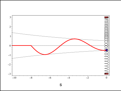
Figure 1. The Lamb model introduced in [19] to describe radiation damping, is a point mass attached to an infinite elastic string and a Hook’s law spring. The point mass evolves as a classical linearly damped oscillator.

Thus the TDD dynamics of (1.11) may be modeled by describing $u(t)$ as one component of an extended vector. The motion of the extended system is reversible, but an irreversible motion of the underlying TDD system results. This is demonstrated in its simplest form by the Lamb model [19] —  see Fig. 1 — in which the energy of an oscillator escapes to infinity along an attached flexible string. For a simple damped harmonic oscillator, the Hamiltonian theory proposed here is precisely the Lamb model, and is otherwise a generalization of the Lamb model, obtained by coupling an infinite classical elastic string to every degree of freedom of the initial Hamiltonian system, illustrating that, from the standpoint of thermodynamics, dissipation in classical linear response is an idealization which assumes infinite heat capacity of (hidden) degrees of freedom.

1.4. Evolution in stress space and a minimal extension

The extension just described is closely related to the extension theory of [7], summarized in §1.1. To understand the relation between the present work and [7], it is useful to recast the evolution (1.11) in stress space. If $\chi(\tau)$ is, say, continuous on $[0,\infty)$ and differentiable for $\tau>0$ then, by (1.11b),

(1.33) $$\partial_{t}Ku(t)\ =\ \partial_{t}f(t)+\int_{0}^{\infty}\mathrm{d}\tau\,\chi(\tau)\partial_{t}f(t-\tau)\mathrm{d}\tau$$

$$=\ \partial_{t}f(t)+\chi(0)f(t)+\int_{0}^{\infty}\mathrm{d}\tau\,[\partial_{\tau}\chi](\tau)f(t-\tau)\mathrm{d}\tau\;.$$

Combining this with (1.11a), we obtain:

(1.34) $$\partial_{t}f(t)\ =\ KJK^{\mathrm{T}}f(t)-\int_{[0,\infty)}\mathrm{d}\tau\,a(\tau)f(t-\tau)+K\rho(t)\;,$$

where $a$ is the operator valued distribution

(1.35) $$a(t)\ =\ \chi(0)\delta(t)\ +\ \partial_{t}\chi(t)\;.$$

The evolution (1.34) is essentially of the form (1.1), with the minor difference that it is defined on a real Hilbert space with a skew-symmetric generator. This is of no consequence, as the main result of [7] holds in this context:

Theorem 1.2.

Suppose given a linear dynamical system described by a point $f$ taking values in a real Hilbert space $H$ which evolves according to (1.1) with a skew-symmetric generator $L=-L^{\mathrm{T}}$. If the friction function $a(\cdot)=\alpha_{\infty}\delta(\cdot)+\alpha(\cdot)$ satisfies the power dissipation condition

(1.36) $$\int_{-\infty}^{\infty}\int_{-\infty}^{\infty}\left(f\left(t\right),a_{e}\left(t-\tau\right)f\left(\tau\right)\right)\,\mathrm{d}t\mathrm{d}\tau\geq 0,$$

for compactly supported continuous functions $f:\mathbb{R}\rightarrow H_{0}$, where

(1.37) $$a_{e}\left(t\right)=2\alpha_{\infty}\delta\left(t\right)+\left\{\begin{array}[]{ccc}\alpha\left(t\right)&\text{if}&t>0\\ \alpha^{\dagger}\left(-t\right)&\text{if}&t<0\end{array}\right.\text{ , }-\infty<t<\infty,$$

then there exist a real Hilbert space extension $\mathcal{H}\overset{I}{\hookleftarrow}H$ and a skew-symmetric operator $\mathcal{L}$ defined on $\mathcal{H}$ such that (1.4) holds.

If, furthermore, the pair $(\mathcal{H},\mathcal{L})$ is minimal, in the sense that $\mathcal{H}$ is the smallest invariant subspace for $\mathcal{L}$ containing the range of $I$, then the pair $(\mathcal{H},\mathcal{L})$ is unique up to transformation by an orthogonal isometry.

Remark: The existence of an extension follows from the results of [7] applied to the complexification of (1.1)(with $f$ a point in $\mathbb{C}H$). This extension will not be minimal in general, but we can restrict the generator to a suitable real subspace to get the minimal extension. Uniqueness may be verified by the arguments of [7]. For completeness we give a more detailed sketch of the proof in Appendix B.

The power dissipation condition (1.14) of the present work implies the PDC (1.36) of [7] for the friction function $a$ defined in (1.35), since

(1.38) $$a_{e}(t)\ =\ \partial_{t}\chi^{\mathrm{o}}(t),$$

with $\chi^{\mathrm{o}}$ the odd extension of the susceptibility $\chi$,

(1.39) $$\chi^{\mathrm{o}}(\tau)\ :=\ \begin{cases}\chi(\tau)\;,&\tau>0\\ -\chi(-\tau)^{\mathrm{T}}\;,&\tau<0\;.\end{cases}$$

In the present work, as in [7], the energy of the dissipative system at time $t$ is $\mathcal{E}(t):=\frac{1}{2}\|f(t)\|^{2}$. For a trajectory $f(\cdot)$ which evolves according to (1.34) this gives a total change in energy from $t=-\infty$ to $t=+\infty$ of

(1.40) $$\int_{-\infty}^{\infty}\partial_{t}\mathcal{E}(t)\mathrm{d}t\ =\ \mathcal{W}_{\mathrm{fr}}[f]+\int_{-\infty}^{\infty}\mathrm{Re}\left(f(t),r(t)\right)\mathrm{d}t,$$

where

(1.41) $$\mathcal{W}_{\mathrm{fr}}[f]:=-\frac{1}{2}\int_{-\infty}^{\infty}\int_{-\infty}^{\infty}\left(f\left(t\right),a_{e}\left(t-\tau\right)f\left(\tau\right)\right)\,\mathrm{d}t\mathrm{d}\tau,$$

It is natural to interpret the two terms on the r.h.s. of (1.40) as the total work done by the frictional and external forces, respectively. Thus, the PDC (1.36) essentially requires that the total work done by frictional forces is always non-positive. This physically natural property also provides a necessary and sufficient condition for an extension of the form (1.3) to exist.

The theorem guarantees the existence of a unique minimal extension of the form (1.3) to the evolution in stress space (1.34). However, for this to be a Hamiltonian extension we must impose a Hamiltonian structure on the dynamical system (1.3). In particular we must express the generator $\mathcal{L}$ as a product

(1.42) $$\mathcal{L}\ =\ \mathcal{K}\mathcal{J}\mathcal{K}^{\mathrm{T}},$$

with $\mathcal{J}$ a symplectic operator. But, given a skew-adjoint operator, there are in general many ways to decompose it in this fashion and thus many ways to impose a Hamiltonian structure on the evolution (1.3). For the resulting structure to be naturally related to the Hamiltonian structure of the original dynamical system (1.10a,1.10b) it is necessary that $\mathcal{K}$ and $\mathcal{J}$ extend the original operators $K$ and $J$ respectively. The main point of this work is to exhibit an explicit Hamiltonian extension with these properties, that may then be used in the analysis of conservation laws for the dissipative system (1.11).

So, by following the motion of the extended stress vector $F(t)=\mathcal{K}U(t)$, we find one extension of the type guaranteed by Theorem 1.2. Indeed, (1.28) implies

(1.43) $$\partial_{t}F(t)\ =\ \mathcal{KJK}^{\mathrm{T}}F(t)\ +\ I_{H}K\rho(t),$$

where the generator $\mathcal{KJK}^{\mathrm{T}}$ is skew-symmetric and has the formal expression

(1.44) $$\mathcal{KJK}^{\mathrm{T}}\ =\ \begin{pmatrix}KJK^{\mathrm{T}}&-T&0\\ T^{\mathrm{T}}&0&\partial_{s}\\ 0&\partial_{s}&0\end{pmatrix}.$$

The solution to (1.43) is easily expressed

(1.45) $$F(t)\ =\ \int_{-\infty}^{t}\mathrm{e}^{(t-t^{\prime})\mathcal{KJK}^{\mathrm{T}}}I_{H}K\rho(t^{\prime})\mathrm{d}t^{\prime},$$

in terms of the one parameter group $\mathrm{e}^{t\mathcal{KJK}^{\mathrm{T}}}$ of orthogonal transformations. By the properties of the QHE, the solution to (1.34) is therefore expressed as

(1.46) $$f(t)\ =\ I_{H}^{\mathrm{T}}F(t)\ =\ \int_{-\infty}^{t}I_{H}^{\mathrm{T}}\mathrm{e}^{(t-t^{\prime})\mathcal{KJK}^{\mathrm{T}}}I_{H}K\rho(t^{\prime})\mathrm{d}t^{\prime}.$$

It is natural to ask is the extension (1.44) is the unique minimal extension of Theorem 1.2. In fact, it is not minimal. Indeed, easily shows that any configuration of the hidden string resulting from a physical driving force $I_{V}\rho(t)$ is symmetric under $s\leftrightarrow-s$. That is, we still have a QHE if we replace $\mathcal{V}$ and $\mathcal{H}$ respectively by

(1.47) $$\mathcal{V}_{s}\ =\ V\oplus\mathcal{S}(\mathbb{R},H)\oplus\mathcal{S}(\mathbb{R},H)\,\text{ and }\mathcal{H}_{s}\ =\ H\oplus\mathcal{S}(\mathbb{R},H)\oplus\mathcal{A}(\mathbb{R},H),$$

with

(1.48) $$\mathcal{S}(\mathbb{R},H) =\ \{\phi\in L^{2}(\mathbb{R},H)\ :\ \phi(s)=\phi(-s)\}$$

$$\mathcal{A}(\mathbb{R},H) =\ \{\phi\in L^{2}(\mathbb{R},H)\ :\ \phi(s)=-\phi(-s)\}.$$

Note that $\mathcal{K}:\mathcal{V}_{s}\rightarrow\mathcal{H}_{s}$ and that $\mathcal{J}:\mathcal{V}_{s}\rightarrow\mathcal{V}_{s}$. If the kernel of the susceptibility $\ker\widehat{\chi}(\omega)$ is non-trivial on a set of positive measure we will see in §2.1 that further reductions are possible.

There is however no harm in working with an extension which is non-minimal, which we do for convenience of notation. Indeed, by (1.45), the solution $F(t)$ remains in the subspace $\mathcal{H}_{0}$ that is the smallest invariant subspace for $\mathcal{K}\mathcal{J}\mathcal{K}^{\mathrm{T}}$ containing the range of $I_{H}$. The restriction of $\mathcal{K}\mathcal{J}\mathcal{K}^{\mathrm{T}}$ to this subspace is the unique minimal extension of Theorem 1.2. Thus even if we employ a non-minimal extension, we effectively work with the unique minimal extension anyway. In §2.1 we give an explicit description of $\mathcal{H}_{0}$ as well as the minimal subspace $\mathcal{V}_{0}\subset\mathcal{V}$ such that $\mathcal{K}:\mathcal{V}_{0}\rightarrow\mathcal{H}_{0}$ and $\mathcal{J}:\mathcal{V}_{0}\rightarrow\mathcal{V}_{0}$.

Finally, we note that even in the minimal extension there is a great deal of freedom to change variables and thus alter the explicit expressions for the extended impedance $\mathcal{K}$. Indeed, given a symplectic operator $\mathcal{J}$ there is a natural symplectic group of symmetries of phase space $\mathcal{V}$ consisting of linear maps $\mathcal{M}$ such that $\mathcal{M}^{\mathrm{T}}\mathcal{J}\mathcal{M}=\mathcal{J}$. Likewise the Hamiltonian $\frac{1}{2}\|\mathcal{K}U\|^{2}$ does not change if we replace the impedance $\mathcal{K}$ by $\mathcal{O}\mathcal{K}$ with $\mathcal{O}$ any orthogonal map of stress space, $\mathcal{O}^{\mathrm{T}}\mathcal{O}=\mathbf{1}.$ Thus the impedance $\mathcal{K}$ is essentially defined only up to re-parameterizations of the form

(1.49) $$\mathcal{K}\ \mapsto\ \mathcal{O}\mathcal{K}\mathcal{M}^{-1},\quad\mathcal{O}^{\mathrm{T}}\mathcal{O}\ =\ \mathbf{1}\text{ and }\mathcal{M}^{\mathrm{T}}\mathcal{J}\mathcal{M}\ =\ \mathcal{J}.$$

We refer to a combined mapping (1.49) of phase and stress space as a symplectic/orthogonal isomorphism. (A symplectic map $\mathcal{M}^{\mathrm{T}}\mathcal{J}\mathcal{M}=\mathcal{J}$ need not be bounded in infinite dimensions, making it somewhat difficult to formulate the change of variables (1.49) in complete generality.)

1.5. Relation with the previous literature

Analysis of a dispersive and dissipative medium based on the construction of its Lagrangian or Hamiltonian is a well established area, see [23, 26, 32, 27, 28] and references therein. However, all of those works have relied on specifying an underlying micro-structure for the material medium, such as an infinite lattice of dipoles as in [23]. In contrast, our approach is phenomenological. Our hidden variables are not “real” microscopic variables as in [23], but describe effective modes which exactly produce a prescribed causal frequency dependent susceptibility. As regards the underlying microscopic theory, our construction can be seen as giving an effective Hamiltonian for those modes well approximated by linear response.

In this section, we compare the approach developed in this paper and our previous work [7] with a number of other efforts to describe dissipative and or dispersive media via extensions (instead of microscopic variables).

1.5.1. Dilation theory

The dilation theory — beginning with the Sz.-Nagy–Foias theory of contractions [43, 44] and Naimark’s theory of positive operator valued measures [31] and subsequently extended by a number of other authors — was the first general method for constructing a spectral theory of dissipative operators and has ultimately provided a complete treatment of dissipative linear systems without dispersion. A key observation of our previous work [7] is that many of the classical tools of dilation theory, in particular Naimark’s theorem, are useful for describing the generic case of dissipative and dispersive systems.

Let us recall the basics of the dilation theory as presented by Pavlov in his extensive review [34] and his more recent work [35]. Although there are a number of approaches to the subject, Pavlov uses Lax-Phillips scattering theory, [25], which provides a conceptually useful picture of the extended operators. That theory assumes the existence of: (i) a dynamical unitary evolution group $U_{t}=\mathrm{e}^{\mathrm{i}\Omega t}$ in a Hilbert space $H$ where $\Omega$ is a self-adjoint operator in $H$; (ii) an incoming subspace $D_{-}\subset H$ invariant under the semi-group $U_{t}$, $t<0$, and an outgoing subspace $D_{+\text{ }}\subset H$ invariant under to the semi-group $U_{t}$, $t>0$. The invariant subspaces $D_{\pm\text{ }}$ (called scattering channels) are assumed to be orthogonal. Then one introduces the observation subspace $Q=H\ominus\left(D_{-}\oplus D_{+}\right)$, assumed to be co-invariant with respect to the unitary group, in the sense that the restriction of $U_{t}$, $t>0$, to $Q$ is a semigroup, i.e.,

(1.50) $$Z_{t}=\left.P_{Q}U_{t}\right|_{Q}=\mathrm{e}^{\mathrm{i}Bt},$$

where $P_{Q}$ is the orthogonal projection onto $Q$.

In many interesting cases the generator $B$ of the semigroup $Z_{t}$ is dissipative, i.e. $\operatorname{Im}B\geq 0$, and the relation (1.50) provides a natural setting for dissipative operators within the Lax-Phillips scattering theory. The dilation theory reverses the Lax-Phillips construction by constructing the Lax-Phillips spaces given $B$ and $Q$. The generator $\Omega$ of the constructed unitary group is called the dilation of $B$ and has the property

(1.51) $$f(B)\ =\ P_{Q}f(\Omega)|_{Q}$$

for suitable analytic functions $f$. Thus the self-adjoint operator $\Omega$ provides an effective spectral theory for the non-self adjoint $B$.

Unfortunately, the dilation theory fails to describe many important physical situations simply because the assumption that dissipation occurs without dispersion, i.e. that $Z_{t}$ is a semi-group, is too restrictive. In systems such as (1.1) dissipation comes with dispersion, and dilation theory applies only in the very special case of instantaneous (Markovian) friction $a\left(t\right)=\alpha_{\infty}\delta\left(t\right)$. Many phenomenological models, such as Lorentz or Debeye dielectric media, employ friction functions which are not instantaneous. For such systems one must use a more general approach as developed in [7] and here.

1.5.2. The work of Tip

The recent papers of Tip [45, 46] is more closely related to this work. For the special case of the EM field in a linear absorptive dielectric, he has given a Hamiltonian formalism involving auxiliary fields similar to our “hidden string.” His formalism made possible an analysis of energy conservation, scattering, and quantization [45] and led to a clarification of the issue of boundary conditions in piecewise constant dielectrics [46]. Stallinga [42] has used this formalism to give formulas for the energy density and stress tensor in dielectric media.

We do not rely on Tip’s work, but the present work follows and parallels it to some extent. In particular, the present paper gives a general context in which some results of [45, 46] may be seen as special cases of results valid in a large class of linear dispersive Hamiltonian systems.

1.5.3. Heat bath and coupling

The evolution equations (1.25, 1.26) describing the hidden string are identical to those of a so-called canonical heat bath as defined in [14, Section 2], [37, Section 2]. As the canonical heat bath as described in [14, Section 2], [37, Section 2] has naturally appeared in our construction, let us look at it in more detail.

The Hamiltonian of our extended system (1.18) can be expressed as a sum of two contributions

(1.52) $$\mathrm{H}(U)\ =\ \mathrm{H}_{\mathrm{sys}}(U)+\mathrm{H}_{\mathrm{str}}(U),$$

the system energy

(1.53) $$\mathrm{H}_{\mathrm{sys}}(U)\ =\ \frac{1}{2}\left\|Ku-T\varphi\right\|_{H}^{2}\ =\ \frac{1}{2}\left\|f\right\|^{2},$$

where $f$ is the kinematical stress as defined by (1.27), and the string energy

(1.54) $$\mathrm{H}_{\mathrm{str}}(U)\ =\ \frac{1}{2}\int_{-\infty}^{\infty}\left[\left\|\theta\left(s\right)\right\|_{H}^{2}+\left\|\partial_{s}\varphi\left(s\right)\right\|_{H}^{2}\right]\,\mathrm{d}s.$$

We conceive of $\mathrm{H}_{\mathrm{sys}}$ as the energy of an open system dynamically coupled to a “heat bath” with energy $\mathrm{H}_{\mathrm{str}}$, described by the hidden string.

The physical concept of a heat bath originates in statstical mechanics. There general considerations show that for a system to behave according to thermodynamics it should be properly coupled to a heat bath. Dynamical models at the mathematical level of rigor were introduced, motivated and described rather recently, see [16, Section 1], [14, Section 2], [37, Section 2] and references therein. According to the references, based on statistical mechanical arguments, the heat bath must be governed by a self-adjoint operator with absolutely continuous spectrum and no gaps, i.e. the spectrum must be the entire real line $\mathbb{R}$, and the spectrum must be of a uniform multiplicity. These requirements lead to a system equivalent to a system with the Hamiltonian $\mathrm{H}_{\mathrm{str}}(\varphi,\theta)$ as in (1.54), [14, Section 2].

Our construction of the unique extended Hamiltonian produces an auxiliary system with Hamiltonian in the form $\mathrm{H}_{\mathrm{str}}(\varphi,\theta)$ as in (1.54) and gives another way to obtain the canonical heat bath as a natural part of the conservative system extending a dissipative and dispersive one under the condition of its causality. In our Hamiltonian setting (1.52) the coupling $\left(Ku,T\varphi\right)$ can be classified as the dipole approximation, [37, Section 1,2], associated with a bilinear form.

1.6. Organization of the paper

The main body of this paper has two parts. The first, comprising Sections 2 – 4, is essentially the physics part of the paper. It consists of a formal derivation of the quadratic Hamiltonian extension (§2), containing all relevant physical details, followed by an application of the extension to TDD wave equations (§3) with Maxwell’s equations for the electro-magnetic field in a TDD medium considered as a detailed example (§4). In particular, in §3 we write the extended Hamiltonian for a TDD wave system as the integral of a local energy density and derive expressions for the energy flux and stress tensor. We also derive general approximations for the time average of these quantities in the special case of an almost mono-chromatic wave. In §4 we specialize these formulas to the Maxwell equations.

The second part, consisting solely of Section 5, is a more detailed mathematical examination of the quadratic Hamiltonian extension. Here we give a precise formulation and proof of the main results leading to Theorem 1.1, with a rigorous analysis of the unbounded operators involved.

The appendices contain supplementary material, including a.) a brief review of notation and spectral theory for operators on real Hilbert spaces, b.) a sketch of the proof of Thm. 1.2, c.) a few examples illustrating the application of our construction to non-linear systems with linear friction and d.) a derivation of the symmetric stress tensor for a system with a Lagrangian density, used in Section 3.

2. Formal construction of a Hamiltonian

We begin by analyzing extended systems of the type outlined in (1.18-1.22), with an unspecified symmetric operator valued coupling function $\varsigma(s)$. It is a simple matter to obtain, via a formal calculation, evolution equations of the form (1.11) for the reduced system. In this way, we get a relation between the susceptibility and the coupling $\varsigma$ — (2.9) below. As it turns out, the symmetry (1.13) and power dissipation (1.14) conditions are necessary and sufficient for inverting (2.9) to write $\varsigma$ as a function of $\chi$.

The extensions we consider are described by a vector coordinate $U$ taking values in the extended phase space $\mathcal{V}=V\oplus L^{2}(\mathbb{R},H)\oplus L^{2}(\mathbb{R},H),$ with $U\in\mathcal{V}$ denoted

(2.1) $$U=\begin{pmatrix}u\\ \theta(s)\\ \varphi(s)\end{pmatrix}\;.$$

Recall that we interpret $\phi(s)$ and $\theta(s)$ as the displacement and momentum density of an $H$-valued string, consistent with the equations of motion (1.24-1.27), namely

(2.2) $$\partial_{t}u(t)\ =\ JK^{\mathrm{T}}f(t)+\rho(t)$$

(2.3) $$\partial_{t}\theta(s,t)\ =\ \partial_{s}^{2}\varphi(s,t)+\varsigma\left(s\right)f(t),$$

(2.4) $$\partial_{t}\varphi(s,t)\ =\ \theta(s,t)$$

with kinematical stress $f$,

(2.5) $$f(t)\ =\ Ku(t)-\int_{-\infty}^{\infty}\mathrm{d}\sigma\varsigma(\sigma)\varphi(\sigma,t)\;.$$

Here we take $\varsigma$ to be an (as yet) unspecified operator valued distribution.

Upon eliminating $\theta$ from (2.3, 2.4), we find that the string displacement $\varphi$ follows a driven wave equation

(2.6) $$\left\{\partial_{t}^{2}-\partial_{s}^{2}\right\}\varphi\left(s,t\right)=\varsigma\left(s\right)f(t).$$

Taking $f$ as given, we solve (2.6) for $\varphi$ with initial values $\lim_{t\rightarrow-\infty}\varphi(t)=0$, $\lim_{t\rightarrow-\infty}\partial_{t}\varphi(t)=0$, corresponding to the string at rest in the distant past:

(2.7) $$\varphi\left(s,t\right)=\frac{1}{2}\int_{0}^{\infty}\mathrm{d}\tau\int_{s-\tau}^{s+\tau}\mathrm{d}\sigma\,\varsigma\left(\sigma\right)f(t-\tau),$$

where we have tacitly assumed that $f(t)$ is integrable. Recalling that $f$ is related to $\varphi$ by (2.5), we obtain the following equation relating $f$ and $u$

(2.8) $$f(t)+\frac{1}{2}\int_{-\infty}^{\infty}\mathrm{d}s\,\int_{0}^{\infty}\mathrm{d}\tau\int_{s-\tau}^{s+\tau}\mathrm{d}\sigma\,\varsigma(s)\varsigma\left(\sigma\right)f(t-\tau)\ =\ Ku(t)\;,$$

which is of the form of the generalized material relation (1.11b) with susceptibility

(2.9) $$\chi\left(\tau\right)=\frac{1}{2}\int_{-\infty}^{\infty}\mathrm{d}s\int_{s-\tau}^{s+\tau}\mathrm{d}\sigma\,\varsigma\left(s\right)\varsigma\left(\sigma\right)\;.$$

Thus, the reduced system described by $u$ is a TDD system of the form (1.11), with susceptibility given by (2.9). To construct a quadratic Hamiltonian extension to (1.11) it essentially suffices to write the string coupling $\varsigma$ as a function of the susceptibility $\chi$ by inverting (2.9). Note that the r.h.s. of (2.9) is a symmetric operator, so the symmetry condition (1.13) is certainly necessary. As we will see the power dissipation condition (1.14) is also necessary, and together the two are sufficient.

Note that (2.9) holds also for $\tau<0$, with $\int_{b}^{a}:=-\int_{a}^{b}$, provided we replace $\chi$ by its odd extension $\chi^{\mathrm{o}}$, defined in (1.39). Differentiating with respect to $\tau$ then gives

(2.10) $$\partial_{\tau}\chi^{\mathrm{o}}(\tau)\ =\ \frac{1}{2}\int_{-\infty}^{\infty}\mathrm{d}s\,\varsigma\left(s\right)\left\{\varsigma\left(s+\tau\right)+\varsigma\left(s-\tau\right)\right\}\;.$$

If $\chi(0+)\neq 0$ then $\chi^{\mathrm{o}}$ has a jump discontinuity at $0$ and (2.10), which holds in the sense of distributions, implies that $\varsigma$ includes a Dirac delta contribution at $s=0$.

To understand the role of the PDC (1.14) here, let us suppose that

(2.11) $$\widehat{\chi}(\omega)=\lim_{\eta\downarrow 0}\widehat{\chi}(\omega+\mathrm{i}\eta)$$

exists and is continuous for $\omega\in\mathbb{R}$, as holds for instance if $\chi\in L^{1}[0,\infty)$. Then the PDC (1.14) implies that

(2.12) $$\omega\mathrm{Im}\widehat{\chi}(\omega)\ \geq\ 0\;,$$

which may be expressed as

(2.13) $$\omega\mathrm{Im}\widehat{\chi}(\omega)\ =\ \frac{1}{2}\widehat{\partial_{\tau}\chi^{\mathrm{o}}}(\omega)\;,$$

where

(2.14) $$\widehat{\chi^{\mathrm{o}}}(\omega)\ =\ \int_{-\infty}^{\infty}\mathrm{d}\tau\,\mathrm{e}^{\mathrm{i}\omega\tau}\chi^{\mathrm{o}}(\tau)\ =\ 2\mathrm{i}\int_{0}^{\infty}\mathrm{d}\tau\sin(\omega\tau)\chi(\tau)\;.$$

To solve for $\varsigma$, we take the Fourier transform of (2.10), which by (2.13) is

(2.15) $$2\omega\mathrm{Im}\widehat{\chi}(\omega)\ =\ \frac{1}{2}\left\{\widehat{\varsigma}(-\omega)\widehat{\varsigma}(\omega)+\widehat{\varsigma}(\omega)\widehat{\varsigma}(-\omega)\right\}\;,$$

with $\widehat{\varsigma}(\omega)=\int_{-\infty}^{\infty}\mathrm{d}s\mathrm{e}^{\mathrm{i}\omega s}\varsigma(s).$ Note that

(2.16) $$\widehat{\varsigma}(\omega)^{\dagger}\ =\ \widehat{\varsigma}(-\omega)\;,$$

where $\bullet^{\dagger}$ denotes the Hermitian conjugate. Therefore (2.15) is the same as

(2.17) $$2\omega\mathrm{Im}\widehat{\chi}(\omega)\ =\ \frac{1}{2}\left\{\widehat{\varsigma}(-\omega)\widehat{\varsigma}(-\omega)^{\dagger}+\widehat{\varsigma}(\omega)\widehat{\varsigma}(\omega)^{\dagger}\right\}\;.$$

Clearly the r.h.s. is non-negative and we see, in particular, that (2.9) implies the power dissipation condition (1.14). (Once the inequality $\omega\mathrm{Im}\widehat{\chi}(\omega)\geq 0$ is known on the real axis, it extends to the entire upper half plane because $\mathrm{Im}\zeta\widehat{\chi}(\zeta)$ is a harmonic function. See (5.32, 5.33) below.)

A solution to (2.9) is not unique. However, there is a unique solution with $\widehat{\varsigma}(\omega)$ a non-negative real symmetric operator for each $\omega$, i.e.,

(2.18) $$\widehat{\varsigma}(\omega)\ =\ \ =\ \widehat{\varsigma}(\omega)^{\mathrm{T}}\ =\ \widehat{\varsigma}(\omega)^{\dagger}\ =\ \widehat{\varsigma}(-\omega),$$

and

(2.19) $$\widehat{\varsigma}(\omega)\ \geq\ 0\;.$$

Indeed, under the symmetry condition (2.18), eq. (2.17) simplifies to

(2.20) $$2\omega\mathrm{Im}\widehat{\chi}(\omega)\ =\ \widehat{\varsigma}(\omega)^{2}\;.$$

(This is consistent since $\mathrm{Im}\widehat{\chi}(\omega)$ is a real operator as we see from the formula $\mathrm{Im}\widehat{\chi}(\omega)=\int_{0}^{\infty}\mathrm{d}t\sin(\omega t)\chi(t)$.) The unique non-negative solution to (2.20) is given by the operator square root,

(2.21) $$\widehat{\varsigma}(\omega)\ =\ \sqrt{2\omega\mathrm{Im}\widehat{\chi}(\omega)}\;.$$

Thus, a quadratic Hamiltonian extension of the system (1.11) is given by (1.18) with the coupling function $\varsigma$ given by Fourier inversion of the r.h.s. of (2.21), i.e.,

(2.22) $$\varsigma(s)\ =\ \frac{1}{2\pi}\int_{\mathbb{R}}\mathrm{d}\omega\,\cos(\omega s)\sqrt{2\omega\mathrm{Im}\widehat{\chi}(\omega)}\;,$$

which is (1.16).

2.1. A minimal extension

The system with Hamiltonian (1.18) has a mechanical interpretation as strings coupled to the degrees of freedom of the underlying TDD system and provides a conceptual picture of the TDD dynamics in terms of absorption and emission of energy by those “hidden” strings. However, for calculations and to describe the minimal extension, it is easier to work with a system in which the string displacement is replaced by its Fourier transform

(2.23) $$\widetilde{\varphi}(\kappa)\ =\ \int_{-\infty}^{\infty}\mathrm{e}^{\mathrm{i}\kappa s}\varphi(s)\mathrm{d}s.$$

To make the change of variables symplectic, we replace the momentum density $\theta$ by

(2.24) $$\widetilde{\theta}(\kappa)\ =\ \frac{1}{2\pi}\int_{-\infty}^{\infty}\mathrm{e}^{\mathrm{i}\kappa s}\theta(s)\mathrm{d}s.$$

The resulting transformation of phase space

(2.25) $$U\ \mapsto\ \mathcal{M}U\ =\ \begin{pmatrix}1&0&0\\ 0&\frac{1}{2\pi}\mathcal{F}&0\\ 0&0&\mathcal{F}\end{pmatrix}U,$$

with $\mathcal{F}f(\kappa)\ =\ \int_{\mathbb{R}}\mathrm{e}^{\mathrm{i}\kappa s}f(s)\mathrm{d}s$, is a symplectic map — $\mathcal{M}\mathcal{J}\mathcal{M}^{\mathrm{T}}=\mathcal{J}$, since $\mathcal{F}^{-1}=\frac{1}{2\pi}\mathcal{F}^{\mathrm{T}}$. Note that the Fourier transform $\mathcal{F}$ maps the symmetric space $\mathcal{S}(\mathbb{R},H)$, defined in (1.48), onto itself, since $\phi(s)=\phi(-s)$ implies that $\mathcal{F}\phi(\kappa)$ is real. Thus $\mathcal{M}$ is well defined as a symplectic map on the reduced phase space $\mathcal{V}_{s}$ (see (1.47)). Correspondingly, we transform stress space by the orthogonal map

(2.26) $$F\ \mapsto\ \mathcal{O}F\ =\ \begin{pmatrix}1&0&0\\ 0&\frac{1}{\sqrt{2\pi}}\mathcal{F}&0\\ 0&0&\frac{1}{\sqrt{2\pi}}\mathrm{i}\mathcal{F}\end{pmatrix}F.$$

The map $\mathrm{i}\mathcal{F}$ maps the anti-symmetric space $\mathcal{A}(\mathbb{R},H)$ (see (1.48)) onto itself, so $\mathcal{O}$ is well defined as an orthogonal map of the reduced stress space $\mathcal{H}_{s}$ (see (1.47)). Together the two transformations amount to an symplectic/orthogonal isomorphism of the form (1.49), and the impedance is transformed to

(2.27) $$\mathcal{K}\ \mapsto\ \widehat{\mathcal{K}}\ =\ \mathcal{O}\mathcal{K}\mathcal{M}^{-1},$$

where

(2.28) $$\widehat{\mathcal{K}}\begin{pmatrix}u\\ \widetilde{\theta}(\kappa)\\ \widetilde{\varphi}(\kappa)\end{pmatrix}\ =\ \begin{pmatrix}K&0&-\frac{1}{2\pi}\widehat{T}\\ 0&\sqrt{2\pi}\mathbf{1}&0\\ 0&0&\frac{1}{\sqrt{2\pi}}\kappa\end{pmatrix}\begin{pmatrix}u\\ \widetilde{\theta}(\kappa)\\ \widetilde{\varphi}(\kappa)\end{pmatrix}.$$

Here

(2.29) $$\widehat{T}\widetilde{\varphi}\ =\ \int_{-\infty}^{\infty}\widehat{\varsigma}(\kappa)\widetilde{\varphi}(\kappa)\mathrm{d}\kappa,$$

where $\widehat{\varsigma}$ was defined in (2.21).

The associated equations of motion, from the Fourier transform of (2.2–2.5), are

(2.30) $$\partial_{t}u(t)\ =\ JK^{\mathrm{T}}f(t)$$

(2.31) $$\partial_{t}\widetilde{\theta}(\kappa,t)\ =\ -\frac{1}{2\pi}\kappa^{2}\widetilde{\varphi}(\kappa,t)+\frac{1}{2\pi}\widehat{\varsigma}(\kappa)f(t)$$

(2.32) $$\partial_{t}\widetilde{\varphi}(\kappa,t)\ =\ 2\pi\widetilde{\theta}(\kappa,t),$$

with

(2.33) $$f(t)\ =\ Ku(t)-\frac{1}{2\pi}\int_{-\infty}^{\infty}\widehat{\varsigma}(\kappa)\widetilde{\varphi}(\kappa,t)\mathrm{d}\kappa.$$

Combining (2.31) and (2.32) we obtain the Fourier Transform of (2.6)

(2.34) $$\partial_{t}^{2}\widetilde{\varphi}(\kappa,t)\ =\ -\kappa^{2}\widetilde{\varphi}(\kappa,t)+\widehat{\varsigma}(\kappa)f(t),$$

with solution

(2.35) $$\widetilde{\varphi}(\kappa,t)\ =\ \widehat{\varsigma}(\kappa)\cdot\left[\int_{-\infty}^{t}\frac{\sin(\kappa(t-t^{\prime}))}{\kappa}f(t^{\prime})\mathrm{d}t^{\prime}\right].$$

Clearly the resulting string displacement satisfies

(2.36) $$\widetilde{\varphi}(\kappa,t)\ \in\ \operatorname{ran}\left(\widehat{\varsigma}(\kappa)\right)\text{ for every }\kappa\in\mathbb{R}.$$

The same holds for the momentum density $\widetilde{\theta}$, since

(2.37) $$\widetilde{\theta}(\kappa,t)\ =\ \partial_{t}\widetilde{\varphi}(\kappa,t)\ =\ 2\pi\widehat{\varsigma}(\kappa)\cdot\left[\int_{-\infty}^{t}\cos(\kappa(t-t^{\prime}))f(t^{\prime})\mathrm{d}t^{\prime}\right].$$

Thus, we may restrict the phase space to the Hilbert space

(2.38) $$\mathcal{V}_{0}\ =\ V\oplus\mathcal{S}_{\widehat{\varsigma}}(\mathbb{R},H)\oplus\mathcal{S}_{\widehat{\varsigma}}(\mathbb{R},H),$$

where

(2.39) $$\mathcal{S}_{\widehat{\varsigma}}(\mathbb{R},H)\ =\ \left\{f\in\mathcal{S}(\mathbb{R},H)\ :\ f(\kappa)\in\operatorname{ran}\left(\widehat{\varsigma}(\kappa)\right)\text{ for every }\kappa\in\mathbb{R}\right\}.$$

We denote by $\mathcal{J}_{0}$ and $\widehat{\mathcal{K}}_{0}$ the restrictions of the symplectic operator $\mathcal{J}$ and impedance $\widehat{\mathcal{K}}$ to $\mathcal{V}_{0}$. Thus $\mathcal{J}_{0}$ still has the block matrix form (1.22) and $\widehat{\mathcal{K}}_{0}$ is defined by the r.h.s. of (2.28) for vectors $U=(u,\widetilde{\theta},\widetilde{\phi})\in\mathcal{V}_{0}$. We consider the impedance $\widehat{\mathcal{K}}_{0}$ as a map from $\mathcal{V}_{0}$ to the restricted stress space

(2.40) $$\mathcal{H}_{0}\ =\ H\oplus\mathcal{S}_{\widehat{\varsigma}}(\mathbb{R},H)\oplus\mathcal{A}_{\widehat{\varsigma}}(\mathbb{R},H)$$

with (see (1.48))

(2.41) $$\mathcal{A}_{\widehat{\varsigma}}(\mathbb{R},H)\ =\ \left\{f\in\mathcal{A}(\mathbb{R},H)\ :\ f(\kappa)\in\operatorname{ran}\left(\widehat{\varsigma}(\kappa)\right)\text{ for every }\kappa\in\mathbb{R}\right\}.$$

Clearly $\mathcal{J}_{0},\widehat{\mathcal{K}}_{0}$ give a quadratic Hamiltonian extension to (1.11). We claim that the resulting extension to (1.34) is the unique minimal extension guaranteed by Theorem 1.2. Indeed the generator has the expression

(2.42) $$\widehat{\mathcal{K}}_{0}\mathcal{J}_{0}\widehat{\mathcal{K}}_{0}^{\mathrm{T}}\ =\ \begin{pmatrix}KJK^{\mathrm{T}}&-\frac{1}{\sqrt{2\pi}}\widehat{T}&0\\ \frac{1}{\sqrt{2\pi}}\widehat{T}^{\mathrm{T}}&0&-\kappa\\ 0&\kappa&0\end{pmatrix},$$

where $[\widehat{T}^{\mathrm{T}}f](\kappa)\ =\ \widehat{\varsigma}(\kappa)f,$ by (2.29). One easily verifies there is no subspace of $\mathcal{H}_{0}$ invariant under $\widehat{\mathcal{K}}_{0}\mathcal{J}_{0}\widehat{\mathcal{K}}_{0}^{\mathrm{T}}$ and containing $H\oplus 0\oplus 0$ (the range of $I_{H}$). Thus:

Theorem 2.1.

There exists a quadratic Hamiltonian extension with $(\mathcal{H},\mathcal{K}\mathcal{J}\mathcal{K}^{\mathrm{T}})$ the unique minimal extension of Theorem 1.2.

For the purpose of calculation it is sometimes useful to take the Fourier-Laplace transform (1.15) with respect to time, setting

(2.43) $$\begin{pmatrix}\widehat{u}(\zeta)\\ \widehat{\theta}(\kappa,\zeta)\\ \widehat{\varphi}(\kappa,\zeta)\end{pmatrix}\ =\ \int_{-\infty}^{\infty}\mathrm{e}^{\mathrm{i}\zeta t}\begin{pmatrix}u(t)\\ \widetilde{\theta}(\kappa,t)\\ \widetilde{\varphi}(\kappa,t)\end{pmatrix}\mathrm{d}t,\quad\mathrm{Im}\zeta>0.$$

We obtain the system of equations

(2.44) $$-\mathrm{i}\zeta\widehat{u}(\zeta)\ =\ JK^{\mathrm{T}}\widehat{f}(\zeta)$$

(2.45) $$-\mathrm{i}\zeta\widehat{\theta}(\kappa,\zeta)\ =\ -\frac{1}{2\pi}\kappa^{2}\widehat{\varphi}(\kappa,\zeta)+\frac{1}{2\pi}\widehat{\varsigma}(\kappa)\widehat{f}(\zeta)$$

(2.46) $$-\mathrm{i}\zeta\widehat{\varphi}(\kappa,\zeta)\ =\ 2\pi\widehat{\theta}(\kappa,\zeta),$$

with

(2.47) $$\widehat{f}(\zeta)\ =\ K\widehat{u}(\zeta)-\frac{1}{2\pi}\int_{-\infty}^{\infty}\widehat{\varsigma}(\kappa)\widehat{\varphi}(\kappa,\zeta)\mathrm{d}\kappa.$$

In particular (2.45, 2.46) together imply

(2.48) $$\widehat{\varphi}(\kappa,\zeta)\ =\ \frac{1}{\kappa^{2}-\zeta^{2}}\widehat{\varsigma}(\kappa)\widehat{f}(\zeta),$$

which, with (2.47), yields

(2.49) $$\widehat{f}(\zeta)+\frac{1}{2\pi}\int_{-\infty}^{\infty}\frac{1}{\kappa^{2}-\zeta^{2}}\widehat{\varsigma}(\kappa)^{2}\mathrm{d}\kappa\widehat{f}(\zeta)\ =\ K\widehat{u}(\zeta).$$

This is suggestive of the identity

(2.50) $$\widehat{\chi}(\zeta)\ =\ \frac{1}{2\pi}\int_{-\infty}^{\infty}\frac{1}{\kappa^{2}-\zeta^{2}}\widehat{\varsigma}(\kappa)^{2}\mathrm{d}\kappa,$$

which holds for $\widehat{\varsigma}$ as in (2.21) as we shall see in the proof of Theorem 5.4 below. In fact, (2.50) is a consequence of the Herglotz-Nevanlina representation for an (operator valued) analytic function in the upper half plane with non-negative imaginary part (see [1, Section 59] and [24, Section 32.3]) or, what is essentially the same, the Kramers-Kronigs relations (see [22, Sec. 62]).

2.2. TDD Lagrangian systems

In many applications the phase space $V$ decomposes naturally as $V_{\mathrm{p}}\oplus V_{\mathrm{q}}$ ($V_{\mathrm{p}}=V_{\mathrm{q}}$), with the symplectic operator in the canonical form:

(2.51) $$J=\begin{pmatrix}0&-\mathbf{1}\\ \mathbf{1}&0\end{pmatrix}\;.$$

The two components of $u=\begin{pmatrix}p\\ q\end{pmatrix}\in V$ are “momentum” and “coordinate” respectively. If the linear map $K$ is block diagonal

(2.52) $$K\ =\ \begin{pmatrix}K_{\mathrm{p}}&0\\ 0&K_{\mathrm{q}}\end{pmatrix}\;,$$

then the linear maps $K_{\mathrm{p}}$ and $K_{\mathrm{q}}$ can be thought of as follows:

$$K_{\mathrm{p}}^{\mathrm{T}}K_{\mathrm{p}}\text{ is the inverse mass (mobility) operator, and }$$

$$K_{\mathrm{q}}^{\mathrm{T}}K_{\mathrm{q}}\text{ is the stiffness (inverse flexibility) operator.}$$

Correspondingly, we suppose that $K_{\mathrm{p}}$ is boundedly invertible, or at least invertible, as otherwise there are “infinitely massive” modes. The equations of motion are

(2.53) $$\partial_{t}\begin{pmatrix}p(t)\\ q(t)\end{pmatrix}\ =\ \begin{pmatrix}-K_{\mathrm{q}}^{\mathrm{T}}f_{\mathrm{q}}(t)\\ K_{\mathrm{p}}^{\mathrm{T}}f_{\mathrm{p}}(t)\end{pmatrix},\quad\begin{pmatrix}f_{\mathrm{p}}(t)\\ f_{\mathrm{q}}(t)\end{pmatrix}\ =\ \begin{pmatrix}K_{\mathrm{p}}p(t)\\ K_{\mathrm{q}}q(t)\end{pmatrix}.$$

A system in this form has an equivalent Lagrangian formulation, with Lagrangian

(2.54) $$\mathrm{L}(q,\partial_{t}q)\ =\ \langle p,\partial_{t}q\rangle-\mathrm{h}(p,q),$$

where we express $p$ as a function of $\partial_{t}q$ using the equation of motion for $q$, i.e.,

(2.55) $$p=\left[K_{\mathrm{p}}^{\mathrm{T}}K_{\mathrm{p}}\right]^{-1}\partial_{t}q.$$

As $K_{\mathrm{p}}$ is boundedly invertible, eq. (2.55) is unambiguous. Thus, the Lagrangian is

(2.56) $$\mathrm{L}(q,\partial_{t}q)\ =\ \frac{1}{2}\left\|\left[K_{\mathrm{p}}^{-1}\right]^{\mathrm{T}}\partial_{t}q\right\|_{H_{\mathrm{p}}}^{2}-\frac{1}{2}\left\|K_{\mathrm{q}}q\right\|_{H_{\mathrm{q}}}^{2},$$

where we have $H=H_{\mathrm{p}}\oplus H_{\mathrm{q}}$ with $K_{\mathrm{w}}\in\mathcal{L}(V_{\mathrm{w}},H_{\mathrm{w}})$, $\mathrm{w}=\mathrm{p,q}$. The trajectory $q(t)$ may be obtained from the Lagrangian by noting that it is a stationary point for the action $\mathrm{A}([q(\cdot)];t_{0},t_{1})=\int_{t_{0}}^{t_{1}}\mathrm{L}(q(t),\partial_{t}q(t))\mathrm{d}t.$ The Euler-Lagrange equation obtained by setting the variation of $\mathrm{A}$ equal to zero is

(2.57) $$\left[K_{\mathrm{p}}^{\mathrm{T}}K_{\mathrm{p}}\right]^{-1}\partial_{t}^{2}q\ =\ -K_{\mathrm{q}}^{\mathrm{T}}K_{\mathrm{q}}q,$$

which is formally equivalent to (1.10a, 1.10b), with $u=\begin{pmatrix}q\\ [K_{\mathrm{p}}^{\mathrm{T}}K_{\mathrm{p}}]^{-1}\partial_{t}q\end{pmatrix}$.

For a Lagrangian system of this form, we generally make the physically natural assumption that an external driving force $\rho(t)$ couples through the r.h.s. of (2.57). That is the equation of motion is

(2.58) $$\left[K_{\mathrm{p}}^{\mathrm{T}}K_{\mathrm{p}}\right]^{-1}\partial_{t}^{2}q(t)\ =\ -K_{\mathrm{q}}^{\mathrm{T}}K_{\mathrm{q}}q(t)+\rho(t),$$

with $\rho(t)\in V_{\mathrm{p}}=V_{\mathrm{q}}$. This amounts to consider the time dependent Lagrangian $\mathrm{L}(q,\partial_{t}q,)+\langle q(t),\rho(t)\rangle_{V_{\mathrm{q}}}$, or Hamiltonian $\mathrm{h}(q,\partial_{t}q)-\langle q(t),\rho(t)\rangle_{V_{\mathrm{q}}}$.

For a TDD system (1.11) with Hamiltonian $\mathrm{h}$ of this form, the extended Hamiltonian (1.18), $\mathrm{H}(U)=\frac{1}{2}\|\mathcal{K}U\|^{2}$, is of the form

(2.59) $$\mathcal{K}\ =\ \begin{pmatrix}K_{\mathrm{p}}&0&0&-T_{\mathrm{p}}\\ 0&K_{\mathrm{q}}&0&-T_{\mathrm{q}}\\ 0&0&1&0\\ 0&0&0&\partial_{s}\end{pmatrix}\;,$$

where $T_{\mathrm{p}}$, $T_{\mathrm{q}}$ are the $p$ and $q$ components of the coupling operator $T$ (see (1.17)):

(2.60) $$T\varphi\ =\ \begin{pmatrix}T_{\mathrm{p}}\varphi\\ T_{\mathrm{q}}\varphi\end{pmatrix}\ =\ \int_{-\infty}^{\infty}\begin{pmatrix}\varsigma_{\mathrm{p}}(s)\\ \varsigma_{\mathrm{q}}(s)\end{pmatrix}\varphi(s)\mathrm{d}s,$$

with momentum and coordinate string coupling functions $\varsigma_{\mathrm{p}}$ and $\varsigma_{\mathrm{q}}$ respectively. Notice that the constitutive relation (2.5) turns into

(2.61) $$f_{\mathrm{q}}=K_{\mathrm{q}}q-T_{\mathrm{q}}\varphi,\ f_{\mathrm{p}}=K_{\mathrm{p}}p-T_{\mathrm{p}}\varphi,$$

readily implying the following representation for the Hamiltonian

(2.62) $$\begin{aligned} \mathrm{H}(U)\ &=\ \frac{1}{2}\left\{\left\|f_{\mathrm{q}}\right\|_{H_{\mathrm{q}}}^{2}+\left\|f_{\mathrm{p}}\right\|_{H_{\mathrm{p}}}^{2}\right\}+\frac{1}{2}\int_{0}^{\infty}\left[\left\|\theta\left(s\right)\right\|_{H}^{2}+\left\|\partial_{s}\varphi\left(s\right)\right\|_{H}^{2}\right]\,\mathrm{d}s\\ &=\ \frac{1}{2}\left\{\left\|K_{\mathrm{q}}q-T_{\mathrm{q}}\varphi\right\|_{H_{\mathrm{q}}}^{2}+\left\|K_{\mathrm{p}}p-T_{\mathrm{p}}\varphi\right\|_{H_{\mathrm{p}}}^{2}\right\}\\ &\quad+\frac{1}{2}\int_{0}^{\infty}\left[\left\|\theta\left(s\right)\right\|_{H}^{2}+\left\|\partial_{s}\varphi\left(s\right)\right\|_{H}^{2}\right]\,\mathrm{d}s,\end{aligned}$$

where $H=H_{\mathrm{q}}\oplus H_{\mathrm{p}}.$

We form a Lagrangian for the extended system, taking $p$ and $\theta$ as momenta,

(2.63) $$\mathrm{L}(q,\varphi,\partial_{t}q,\partial_{t}\varphi)\ =\ \langle p,\partial_{t}q\rangle+\langle\theta,\partial_{t}\varphi\rangle-\mathrm{H}(p,q,\theta,\varphi).$$

where we must write $p$ and $\theta$ as functions of $\partial_{t}q$, $\partial_{t}\varphi$ and $\varphi$,

(2.64) $$\theta\ =\ \partial_{t}\varphi,\text{ and }p\ =\ \left[K_{\mathrm{p}}^{\mathrm{T}}K_{\mathrm{p}}\right]^{-1}\partial_{t}q+K_{\mathrm{p}}^{-1}T_{\mathrm{p}}\varphi,$$

using the equations of motion. Thus the above and (2.63) imply

(2.65) $$\mathrm{L}(q,\varphi,\partial_{t}q,\partial_{t}\varphi)\ =\ \frac{1}{2}\left\|\left[K_{\mathrm{p}}^{-1}\right]^{\mathrm{T}}\partial_{t}q\right\|_{H_{\mathrm{p}}}^{2}+\left\langle\left[K_{\mathrm{p}}^{-1}\right]^{\mathrm{T}}\partial_{t}q,T_{\mathrm{p}}\varphi\right\rangle_{H_{\mathrm{p}}}\\ +\frac{1}{2}\int_{-\infty}^{\infty}\left\|\partial_{t}\varphi(s)\right\|_{H}^{2}\mathrm{d}s-\frac{1}{2}\left\|K_{\mathrm{q}}q-T_{\mathrm{q}}\varphi\right\|^{2}_{H_{\mathrm{q}}}-\frac{1}{2}\int_{-\infty}^{\infty}\left\|\partial_{s}\varphi(s)\right\|_{H}^{2}\mathrm{d}s.$$

The Lagrangian form of the equations of motion, with driving force $\rho$, is

(2.66) $$\partial_{t}\left\{\left[K_{\mathrm{p}}^{\mathrm{T}}K_{\mathrm{p}}\right]^{-1}\partial_{t}q(t)+K_{\mathrm{p}}^{-1}\int_{-\infty}^{\infty}\varsigma_{\mathrm{p}}(s)\varphi(s,t)\mathrm{d}s\right\}\ =\ -K_{\mathrm{q}}^{\mathrm{T}}f_{\mathrm{q}}(t)+\rho(t),$$

(2.67) $$\partial_{t}^{2}\varphi(s,t)\ =\ \partial_{s}^{2}\varphi(s,t)+\varsigma_{\mathrm{q}}(s)f_{\mathrm{q}}(t)-\varsigma_{\mathrm{p}}(s)\left[K_{\mathrm{p}}^{-1}\right]^{\mathrm{T}}\partial_{t}q(t),$$

with

(2.68) $$f_{\mathrm{q}}(t)\ =\ K_{\mathrm{q}}q(t)-\int_{-\infty}^{\infty}\varsigma_{\mathrm{q}}(s)\varphi(s,t)\mathrm{d}s.$$

3. Local TDD Lagragians and conserved currents

Many physical systems of interest are described by wave motion of vector valued fields, with the coordinate variable $u$ a function of the position $\vec{r}\in\mathbb{R}^{d}$ (usu. $d=3$) valued in a Hilbert space $\widehat{V}$. That is, phase space $V=L^{2}(\mathbb{R}^{d};\widehat{V})$. Of particular interest are systems with a Hamiltonian that is an integral over $\mathbb{R}^{d}$ of a density, whose value at a point $\vec{r}$ is a function of the field $u(\vec{r})$ and its derivatives at the point $\vec{r}$. In this section we focus on extended TDD Lagrangian systems of this type with $u(\vec{r})=(p(\vec{r}),q(\vec{r}))$ and the symplectic operator $J$ in the canonical representation (2.51).

That is, we take a system of the type considered in §2.2 and suppose the spaces $V_{\mathrm{q}}=V_{\mathrm{p}}$ and $H_{\mathrm{p,q}}$ are of the form

(3.1) $$V_{\mathrm{q}}=L^{2}(\mathbb{R}^{d},V_{0})\quad\text{and}\quad H_{\mathrm{w}}=L^{2}(\mathbb{R}^{d},H_{\mathrm{w}}^{0}),\quad\mathrm{w}=\mathrm{p,q},$$

with $V_{0}$, $H_{\mathrm{p,q}}^{0}$ real Hilbert spaces. So the coordinate $q$ is a vector field $q(\vec{r})\in V_{0}$. We suppose further that the impedance operator $K$ is of the form

(3.2) $$K\begin{pmatrix}p\\ q\end{pmatrix}(\vec{r})\ =\ \begin{pmatrix}K_{\mathrm{p}}(\vec{r})&0\\ 0&K_{\mathrm{q}}(\vec{r})+\mathbf{Y}_{i}(\vec{r})\cdot\partial_{i}\end{pmatrix}\begin{pmatrix}p\\ q\end{pmatrix}(\vec{r}),$$

where repeated indices are summed from $i=1,\ldots,d$. For each $\vec{r}$, $K_{\mathrm{p}}(\vec{r})$ and $K_{\mathrm{q}}(\vec{r})$, $\mathbf{Y}_{i}(\vec{r})$, $i=1,...,d$ are bounded operators from $V_{0}$ to $H_{\mathrm{p}}^{0}$ and $H_{\mathrm{q}}^{0}$ respectively and $\partial_{i}=\partial/\partial_{\vec{r}_{i}}$. This form covers classical linear elastic, acoustic and dielectric media.

The system, in the absence of dissipation, is governed by a Lagrangian

(3.3) $$\mathrm{L}(q,\partial_{t}q)\ =\ \int_{\mathbb{R}^{d}}\mathsf{L}(q(\vec{r}),\nabla q(\vec{r}),\partial_{t}q(\vec{r}))\mathrm{d}^{d}\vec{r},$$

with a Lagrangian density second order in the coordinate $q(\vec{r})$ and first derivatives:

(3.4) $$\mathsf{L}(q(\vec{r}),\nabla q(\vec{r}),\partial_{t}q(\vec{r}))\\ =\ \frac{1}{2}\left\{\left\|\left[K_{\mathrm{p}}(\vec{r})^{\mathrm{T}}\right]^{-1}\partial_{t}q(\vec{r})\right\|^{2}-\left\|K_{\mathrm{q}}(\vec{r})q(\vec{r})+\mathbf{Y}(\vec{r})\cdot\nabla q(\vec{r})\right\|^{2}\right\}.$$

By a suitable choice of $K_{\mathrm{p},\mathrm{q}}$ and $\mathbf{Y}$ we can obtain any Lagrangian density of the form $\mathsf{L}=T(\partial_{t}q)-V(q,\nabla q)$ with $T$ and $V$ homogeneous of degree two.

Now suppose there is time dispersion and dissipation in the system so that the equations of motion and material relations according to (1.11) and (3.2) are

(3.5) $$\partial_{t}\begin{pmatrix}p(\vec{r},t)\\ q(\vec{r},t)\end{pmatrix}\ =\ \begin{pmatrix}\ -K_{\mathrm{q}}(\vec{r})^{\mathrm{T}}f_{\mathrm{q}}(\vec{r},t)+\partial_{i}\left\{\mathbf{Y}_{i}(\vec{r})^{\mathrm{T}}f_{\mathrm{q}}(\vec{r},t)\right\}\\ K_{\mathrm{p}}^{\mathrm{T}}f_{\mathrm{p}}(\vec{r},t)\end{pmatrix}$$

(3.6) $$\begin{pmatrix}f_{\mathrm{p}}(\vec{r},t)\\ f_{\mathrm{q}}(\vec{r},t)\end{pmatrix}\ +\int_{0}^{\infty}\chi(\tau;\vec{r})\begin{pmatrix}f_{\mathrm{p}}(\vec{r},t-\tau)\\ f_{\mathrm{q}}(\vec{r},t-\tau)\end{pmatrix}\,\mathrm{d}\tau\ =\ \begin{pmatrix}K_{\mathrm{p}}p(\vec{r},t)\\ K_{\mathrm{q}}q(\vec{r},t)+\mathbf{Y}_{i}(\vec{r})\partial_{i}q(\vec{r},t)\end{pmatrix},$$

with $\chi(\tau;\vec{r})$ a $\mathcal{B}(H_{\mathrm{p}}^{0}\oplus H_{\mathrm{q}}^{0})$ valued susceptibility function. The string coupling operators constructed above then fiber over $\mathbb{R}^{d}$ in the same way

(3.7) $$\left[\varsigma_{\mathrm{p}}(s)p\right](\vec{r})\ =\ \varsigma_{\mathrm{p}}(s,\vec{r})p(\vec{r}),\quad\left[\varsigma_{\mathrm{q}}(s)q\right](\vec{r})\ =\ \varsigma_{\mathrm{q}}(s,\vec{r})q(\vec{r}),$$

and the extended Lagrangian (2.65) is the integral of a Lagrangian density:

(3.8) $$\mathrm{L}(Q,\partial_{t}Q)\ =\ \int_{\mathrm{R}^{d}}\mathsf{L}(Q(\vec{r}),\nabla Q(\vec{r}),\partial_{t}Q(\vec{r}))\mathrm{d}^{d}\vec{r},$$

where $Q(\vec{r})=(q(\vec{r}),\varphi(s,\vec{r}))$ and

(3.9) $$\mathsf{L}(Q(\vec{r}),\nabla Q(\vec{r}),\partial_{t}Q(\vec{r}))\\ =\ \frac{1}{2}\left\|\left[K_{\mathrm{p}}^{\mathrm{T}}(\vec{r})\right]^{-1}\partial_{t}q(\vec{r})\right\|_{H_{\mathrm{p}}^{0}}^{2}+\left\langle\left[K_{\mathrm{p}}^{\mathrm{T}}(\vec{r})\right]^{-1}\partial_{t}q(\vec{r}),\int_{-\infty}^{\infty}\varsigma_{\mathrm{p}}(s,\vec{r})\varphi(s,\vec{r})\mathrm{d}s\right\rangle_{H_{\mathrm{p}}^{0}}\\ +\frac{1}{2}\int_{-\infty}^{\infty}\left\|\partial_{t}\varphi(s,\vec{r})\right\|_{H_{\mathrm{p}}^{0}\oplus H_{\mathrm{q}}^{0}}^{2}\mathrm{d}s-\frac{1}{2}\int_{-\infty}^{\infty}\left\|\partial_{s}\varphi(s,\vec{r})\right\|_{H_{\mathrm{p}}^{0}\oplus H_{\mathrm{q}}^{0}}^{2}\mathrm{d}s\\ -\left\|K_{\mathrm{q}}(\vec{r})q(\vec{r})+\mathbf{Y}(\vec{r})\cdot\nabla q(\vec{r})-\int_{-\infty}^{\infty}\varsigma_{\mathrm{q}}(s,\vec{r})\varphi(s,\vec{r})\mathrm{d}s\right\|_{H_{\mathrm{q}}^{0}}^{2}.$$

Remark: $\varphi$ is an element of $L^{2}(\mathbb{R},H)$ with $H=H_{\mathrm{p}}\oplus H_{\mathrm{q}}=L^{2}(\mathbb{R}^{d},H_{\mathrm{p}}^{0}\oplus H_{\mathrm{q}}^{0})$. We identify $L^{2}(\mathbb{R},H)$ with $L^{2}(\mathbb{R}\times\mathbb{R}^{d},H_{\mathrm{p}}^{0}\oplus H_{\mathrm{q}}^{0})$, writing $\varphi$ as $(s,\vec{r})\mapsto\varphi(s,\vec{r})\in H_{\mathrm{p}}^{0}\oplus H_{\mathrm{q}}^{0}$.

In Appendix D we recall some basic constructions for a system with a Lagrangian density. In particular, we obtain suitable expressions for the energy flux vector and the stress tensor of a homogeneous system. In this section, we apply the expressions derived there to the extended TDD Lagrangian (3.9)

3.1. Energy density and flux

Because $\mathsf{L}$ does not depend explicitly on time, the total energy, which can be expressed as the integral of a density (see (D.4))

(3.10) $$\mathcal{E}\ =\ \int_{\mathrm{R}^{d}}\mathsf{H}(\vec{r},t)\mathrm{d}^{d}\vec{r},$$

is conserved (in the absence of an external driving force). The value of the total energy $\mathcal{E}$ is, of course, just the extended Hamiltonian $\mathrm{H}$ evaluated “on-shell,” at a field configuration evolving according to the equations of motion.

We can express the energy density $\mathsf{H}$ as a sum of two contributions

(3.11) $$\mathsf{H}(\vec{r},t)\ =\ \mathsf{H}_{\mathrm{sys}}(\vec{r},t)+\mathsf{H}_{\mathrm{str}}(\vec{r},t),$$

which we interpret as the energy density of the TDD system and the heat bath, as described by the hidden strings, respectively. Here

(3.12) $$\mathsf{H}_{\mathrm{str}}(\vec{r},t)\ =\ \frac{1}{2}\int_{-\infty}^{\infty}\left\|\partial_{s}\varphi(s,\vec{r},t)\right\|_{H_{\mathrm{p}}^{0}\oplus H_{\mathrm{q}}^{0}}\mathrm{d}s+\frac{1}{2}\int_{-\infty}^{\infty}\left\|\theta(s,\vec{r},t)\right\|_{H_{\mathrm{p}}^{0}\oplus H_{\mathrm{q}}^{0}}\mathrm{d}s,$$

with $\theta(s,\vec{r},t)=\partial_{t}\varphi(s,\vec{r},t)$, and

(3.13) $$\mathsf{H}_{\mathrm{sys}}(\vec{r},t)\ =\ \frac{1}{2}\left\|f_{\mathrm{p}}(\vec{r},t)\right\|_{H_{\mathrm{p}}^{0}}^{2}+\frac{1}{2}\left\|f_{\mathrm{q}}(\vec{r},t)\right\|_{H_{\mathrm{q}}^{0}}^{2},$$

with $f_{\mathrm{q,p}}$ the coordinate and momentum parts of the kinematical stress,

(3.14) $$f_{\mathrm{q}}(\vec{r})\ =\ K_{\mathrm{q}}(\vec{r})q(\vec{r})+\mathbf{Y}(\vec{r})\cdot\nabla q(\vec{r})-\int_{-\infty}^{\infty}\varsigma_{\mathrm{q}}(s,\vec{r})\varphi(s,\vec{r})\mathrm{d}s,$$

and

(3.15) $$f_{\mathrm{p}}(\vec{r})\ =\ \left[K_{\mathrm{p}}^{\mathrm{T}}(\vec{r})\right]^{-1}\partial_{t}q(\vec{r},t)\ =\ K_{\mathrm{p}}(\vec{r})p(\vec{r},t)-\int_{-\infty}^{\infty}\varsigma_{\mathrm{p}}(s,\vec{r})\varphi(s,\vec{r},t)\mathrm{d}s,$$

as follows from (2.5), (3.2) and (3.6). By (3.11–3.13), $\mathsf{H}_{\mathrm{sys}}$ includes the interaction energy between the system and the hidden strings.

The energy density, expressed in canonical coordinates, $\mathsf{H}(\vec{r},t)=$ $\mathsf{H}\bigl{(}q(\vec{r},t),$ $\nabla q(\vec{r},t),$ $\varphi(\cdot,\vec{r},t),$ $p(\vec{r},t),$ $\theta(\cdot,\vec{r},t)\bigr{)}$, is also the Hamiltonian density. The equations of motion can be recovered by variation

(3.16) $$\partial_{t}q(\vec{r},t) =\frac{\delta\mathsf{H}}{\delta p}(\vec{r},t)=K_{\mathrm{p}}^{\mathrm{T}}(\vec{r})f_{\mathrm{p}}(\vec{r},t),$$

(3.17) $$\partial_{t}p(\vec{r},t) =\left\{-\frac{\delta\mathsf{H}}{\delta q}+\partial_{i}\frac{\delta\mathsf{H}}{\delta\partial_{i}q}\right\}(\vec{r},t)=-K_{\mathrm{q}}^{\mathrm{T}}(\vec{r})f_{\mathrm{q}}(\vec{r},t)+\partial_{i}\mathbf{Y}_{i}^{\mathrm{T}}(\vec{r})f_{\mathrm{q}}(\vec{r},t),$$

(3.18) $$\partial_{t}\theta(s,\vec{r},t) =-\frac{\delta\mathsf{H}}{\delta\varphi(s)}(\vec{r},t)$$

$$=\partial_{s}^{2}\varphi(s,\vec{r},t)+\varsigma_{\mathrm{p}}^{\mathrm{T}}(\vec{r},s)f_{\mathrm{p}}(\vec{r},t)+\varsigma_{\mathrm{q}}^{\mathrm{T}}(\vec{r},s)f_{\mathrm{q}}(\vec{r},t)$$

(3.19) $$\partial_{t}\varphi(s,\vec{r},t) =\frac{\delta\mathsf{H}}{\delta\theta(s)}(\vec{r},t)=\theta(s,\vec{r},t).$$

If the system is driven by an external force $\rho(\vec{r},t)\in V_{0}$, we replace (3.17) by

(3.20) $$\partial_{t}p(\vec{r},t)\ =\ -K_{\mathrm{q}}^{\mathrm{T}}(\vec{r})f_{\mathrm{q}}(\vec{r},t)+\partial_{i}\mathbf{Y}_{i}^{\mathrm{T}}(\vec{r})f_{\mathrm{q}}(\vec{r},t)+\rho(\vec{r},t).$$

When the driving force vanishes, the total energy is conserved and the energy density satisfies a local conservation law

(3.21) $$\partial_{t}\mathsf{H}(\vec{r},t)+\partial_{i}\mathbf{S}_{i}(\vec{r},t)\ =\ 0,$$

with $\mathbf{S}$ the energy flux vector, an expression for which is derived Appendix D. For the present case the energy flux is (see (D.5))

(3.22) $$\mathbf{S}_{i}(\vec{r},t)=-\langle\partial_{t}q(\vec{r},t),\mathbf{Y}_{i}^{\mathrm{T}}(\vec{r})f_{\mathrm{q}}(\vec{r},t)\rangle_{V_{0}}=-\langle K_{\mathrm{p}}^{\mathrm{T}}(\vec{r})f_{\mathrm{p}}(\vec{r},t),\mathbf{Y}_{i}^{\mathrm{T}}(\vec{r})f_{\mathrm{q}}(\vec{r},t)\rangle_{V_{0}}.$$

With a non-zero driving force, one has

(3.23) $$\partial_{t}\mathsf{H}(\vec{r},t)+\partial_{i}\mathbf{S}_{i}(\vec{r},t)\ =\ \langle\partial_{t}q(\vec{r},t),\rho(\vec{r},t)\rangle_{V_{0}}$$

in place of (3.21) (see Theorem D.2). Thus

(3.24) $$\partial_{t}\mathcal{E}\ =\ \int_{-\mathbb{R}^{d}}\langle\partial_{t}q(\vec{r},t),\rho(\vec{r},t)\rangle_{V_{0}}\mathrm{d}^{d}\vec{r},$$

consistent with our interpretation of $\langle\partial_{t}q(\vec{r},t),\rho(\vec{r},t)\rangle_{V_{0}}$ as the power density of the external force.

We conceive of the four vector fields $p(\vec{r},t)$, $q(\vec{r},t)$, $f_{\mathrm{p}}(\vec{r},t)$, and $f_{\mathrm{q}}(\vec{r},t)$ as specifying the “state” of the reduced TDD system. By (3.22), the energy flux at time $t$ is a function of these fields evaluated at time $t$. The energy density depends in a more essential way on the configuration of the hidden strings. Nonetheless, we may use (3.23) to give a definition of the energy density intrinsic to the TDD system by writing it as integral over the history of the system, namely

(3.25) $$\mathsf{H}(\vec{r},t)\ =\ \int_{-\infty}^{t}\left\{-\partial_{i}\mathbf{S}_{i}(\vec{r},t^{\prime})+\langle\partial_{t}q(\vec{r},t^{\prime}),\rho(\vec{r},t^{\prime})\rangle_{V_{0}}\right\}\mathrm{d}t^{\prime},$$

if the energy density was zero at $t=-\infty$, i.e. the system and medium were at rest.

3.2. Homogeneity, isotropy, wave momentum and the stress tensor

Suppose the extended TDD system has a Lagrangian density (3.9) which is homogeneous — invariant under spatial translations. Then the total wave momentum $\mathbf{P}$ is conserved, and there is a corresponding conserved current, the wave momentum density $\mathbf{p}(\vec{r},t)$, analyzable using Noether’s Theorem (see [27, Section 5.5]). If the Lagrangian density is also isotropic — invariant under spatial rotations —, then the anti-symmetric tensor of angular momentum about the origin $\mathsf{M}_{i,j}$ is conserved. In appendix D, following [3], we recall the formulation of the symmetric stress tensor $\mathsf{T}$ and wave momentum density $\mathbf{p}$ for a homogeneous and isotropic system.

To say that the Lagrangian in (3.9) is isotropic, we must specify how $q$ and $\varphi$ transform under rotations. Thus we suppose given representations $\Upsilon$ and $\Upsilon_{\mathrm{w}}$, $\mathrm{w}=\mathrm{p,q}$, of the rotation group $\mathsf{SO}(d)$ by orthogonal operators in $\mathcal{B}(V_{0})$ and $\mathcal{B}(H_{\mathrm{w}}^{0})$, $\mathrm{w}=\mathrm{p,q}$, respectively, so that under a global rotation of the coordinate system about the origin,

(3.26) $$\vec{r}\,^{\prime}\ =\ R\cdot\vec{r}$$

with $R\in\mathsf{SO}(d)$ an orthogonal matrix, the fields $q$ and $\varphi$ transform as

(3.27) $$q^{\prime}(\vec{r}\,^{\prime})\ =\ \Upsilon(R)q(R^{-1}\vec{r}\,^{\prime})$$

and

(3.28) $$\varphi^{\prime}(s,\vec{r}\,^{\prime})\ =\ \begin{pmatrix}\Upsilon_{\mathrm{p}}(R)&0\\ 0&\Upsilon_{\mathrm{q}}(R)\end{pmatrix}\varphi(s,R^{-1}\vec{r}\,^{\prime}).$$

(Recall that $\varphi$ is $H_{\mathrm{p}}\oplus H_{\mathrm{q}}$-valued.) The representations $\Upsilon$ and $\Upsilon_{\mathrm{p},\mathrm{q}}$ are specified by families of skew-adjoint operators $g_{i,j}$ and $g_{i,j}^{\mathrm{w}}$, $\mathrm{w}=\mathrm{p,q}$, on $V_{0}$ and $H_{\mathrm{w}}^{0}$, $\mathrm{w}=\mathrm{p,q}$, respectively, $i,j=1,...,d$. A rotation $R=\mathrm{e}^{\omega}$, with $\omega$ an anti-symmetric matrix, has representatives (see appendix D):

(3.29) $$\Upsilon(\mathrm{e}^{\omega})\ =\ \mathrm{e}^{\frac{1}{2}\omega_{i,j}g_{i,j}},\quad\Upsilon_{\mathrm{w}}(\mathrm{e}^{\omega})\ =\ \mathrm{e}^{\frac{1}{2}\omega_{i,j}g_{i,j}^{\mathrm{w}}}\quad(\text{summation convention}).$$

In addition to being skew-adjoint, the operators $g_{i,j}$ and $g_{i,j}^{\mathrm{p},\mathrm{q}}$ satisfy

(3.30) $$g_{i,j}^{\sharp}\ =\ -g_{j,i}^{\sharp},\\ \text{and}\quad g_{i,j}^{\sharp}g_{i^{\prime},j^{\prime}}^{\sharp}-g_{i^{\prime},j^{\prime}}^{\sharp}g_{i,j}^{\sharp}\ =\ -\delta_{i,i^{\prime}}g_{j,j^{\prime}}^{\sharp}+\delta_{i,j^{\prime}}g_{j,i^{\prime}}^{\sharp}+\delta_{j,i^{\prime}}g_{i,j^{\prime}}^{\sharp}-\delta_{j,j^{\prime}}g_{i,i^{\prime}}^{\sharp}.$$

Since $V_{0}$ and $H_{\mathrm{p},\mathrm{q}}$ are finite dimensional in our application to the Maxwell equations below, we assume $g_{i,j}$ and $g_{i,j}^{\mathrm{w}}$ are bounded for simplicity.

Definition 3.1.

The Lagrangian density (3.9) is homogeneous if $K_{\mathrm{p,q}}(\vec{r})$, $\mathbf{Y}(\vec{r})$, and $\varsigma_{\mathrm{p,q}}(\vec{r},s)$ are independent of $\vec{r}$, and is isotropic if

(3.31) $$K_{\mathrm{w}}g_{i,j}\ =\ g_{i,j}^{\mathrm{w}}K_{\mathrm{w}},\quad\mathrm{w}=\mathrm{p,q}$$

(3.32) $$\mathbf{Y}_{k}g_{i,j}\ =\ g_{i,j}^{\mathrm{q}}\mathbf{Y}_{k}+\delta_{j,k}\mathbf{Y}_{i}-\delta_{i,k}\mathbf{Y}_{j}$$

and

(3.33) $$\varsigma_{\mathrm{w}}(s)\begin{pmatrix}g_{i,j}^{\mathrm{p}}&0\\ 0&g_{i,j}^{\mathrm{q}}\end{pmatrix}\ =\ g_{i,j}^{\mathrm{w}}\varsigma_{\mathrm{w}}(s),\quad\mathrm{w}=\mathrm{p,q}.$$

Remarks: i.) In Appendix D we give more general definitions D.1 and D.2, which are consistent with 3.1. ii.) The last two terms on the r.h.s. of (3.32) result from the fact that $\mathbf{Y}_{i}$ appear coupled with a spatial derivative in the Lagrangian (3.9). iii.) Recall that $\varsigma_{\mathrm{w}}(s,\vec{r}):H_{\mathrm{p}}\oplus H_{\mathrm{q}}\rightarrow H_{\mathrm{w}}$.

Theorem D.1 below gives the following expressions for the wave momentum density $\mathbf{p}$ and stress tensor $\mathsf{T}$, expressed here in canonical coordinates:

(3.34) $$\mathbf{p}_{i}(\vec{r},t)\ =\ \left\langle\partial_{i}q(\vec{r},t),p(\vec{r},t)\right\rangle_{V_{0}}\\ +\int_{-\infty}^{\infty}\left\langle\partial_{i}\varphi(s,\vec{r},t),\theta(s,\vec{r},t)\right\rangle_{H_{\mathrm{p}}^{0}\oplus H_{\mathrm{q}}^{0}}\mathrm{d}s-\partial_{j}\Phi_{i,j}(\vec{r},t),$$

(3.35) $$\mathsf{T}_{i,j}(\vec{r},t)\\ =\ -\left\langle\partial_{i}q(\vec{r},t),\mathbf{Y}_{j}^{\mathrm{T}}f_{\mathrm{q}}(\vec{r},t)\right\rangle_{V_{0}}-\delta_{i,j}\mathsf{L}(\vec{r},t)+\partial_{t}\Phi_{i,j}+\partial_{k}\Psi_{i,j,k}(\vec{r},t),$$

where $f_{\mathrm{p,q}}$ are defined in (3.14, 3.15), $\mathsf{L}$ is the Lagrangian density

(3.36) $$\mathsf{L}(\vec{r},t)\ =\ \left\langle\mathsf{K}_{\mathrm{p}}^{\mathrm{T}}f_{\mathrm{p}}(\vec{r},t),p(\vec{r},t)\right\rangle_{H_{\mathrm{p}}^{0}}-\frac{1}{2}\left\|f_{\mathrm{p}}(\vec{r},t)\right\|_{H_{\mathrm{p}}^{0}}^{2}-\frac{1}{2}\left\|f_{\mathrm{q}}(\vec{r},t)\right\|_{H_{\mathrm{q}}^{0}}^{2}\\ +\frac{1}{2}\int_{-\infty}^{\infty}\left\|\theta(\vec{r},s,t)\right\|_{H_{\mathrm{p}}^{0}}^{2}\mathrm{d}s-\frac{1}{2}\int_{-\infty}^{\infty}\left\|\partial_{s}\varphi(s,\vec{r})\right\|_{H_{\mathrm{p}}^{0}\oplus H_{\mathrm{q}}^{0}}^{2}\mathrm{d}s,$$

and

(3.37) $$\Phi_{i,j}(\vec{r},t)\ =\ \frac{1}{2}\left\langle g_{i,j}q(\vec{r},t),p(\vec{r},t)\right\rangle_{V^{0}}\\ +\frac{1}{2}\int_{-\infty}^{\infty}\left\langle\begin{pmatrix}g_{i,j}^{\mathrm{p}}&0\\ 0&g_{i,j}^{\mathrm{q}}\end{pmatrix}\varphi(s,\vec{r},t),\theta(s,\vec{r},t)\right\rangle_{H_{\mathrm{p}}^{0}\oplus H_{\mathrm{q}}^{0}}\mathrm{d}s,$$

(3.38) $$\Psi_{i,j,k}(\vec{r},t)\ =\ -\frac{1}{2}\left\langle g_{i,j}q(\vec{r},t),\mathbf{Y}_{k}^{\mathrm{T}}f_{\mathrm{q}}(\vec{r},t)\right\rangle_{V_{0}}\\ +\frac{1}{2}\left\langle g_{j,k}q(\vec{r},t),\mathbf{Y}_{i}^{\mathrm{T}}f_{\mathrm{q}}(\vec{r},t)\right\rangle_{V_{0}}+\frac{1}{2}\left\langle g_{i,k}q(\vec{r},t),\mathbf{Y}_{j}^{\mathrm{T}}f_{\mathrm{q}}(\vec{r},t)\right\rangle_{V_{0}}.$$

As the system is homogeneous, the total wave momentum

(3.39) $$\mathbf{P}\ =\ \int_{\mathbb{R}^{d}}\mathbf{p}(\vec{r},t)\mathrm{d}^{d}\vec{r}$$

is conserved in the absence of a driving force, and the wave momentum density satisfies the local conservation law

(3.40) $$\partial_{t}\mathbf{p}_{i}(\vec{r},t)+\partial_{j}\mathsf{T}_{i,j}(\vec{r},t)\ =\ 0.$$

With a driving force, (3.40) is modified to (see Theorem D.2)

(3.41) $$\partial_{t}\mathbf{p}_{i}(\vec{r},t)+\partial_{j}\mathsf{T}_{i,j}(\vec{r},t)\ =\ \left\langle\partial_{i}q(\vec{r},t),\rho(\vec{r},t)\right\rangle_{V_{0}},$$

and thus

(3.42) $$\partial_{t}\mathbf{P}\ =\ \int_{\mathbb{R}^{d}}\left\langle\partial_{i}q(\vec{r},t),\rho(\vec{r},t)\right\rangle_{V_{0}}\mathrm{d}^{d}\vec{r}.$$

Due to the term $\partial_{t}\Phi_{i,j}$ in the definition of the stress tensor (3.35), the driving force also modifies $\mathsf{T}$. If $\mathsf{T}_{i,j}^{0}(\vec{r},t)$ is the stress tensor with $\rho(\vec{r},t)=0$, then

(3.43) $$\mathsf{T}_{i,j}(\vec{r},t)\ =\ \mathsf{T}_{i,j}^{0}(\vec{r},t)+\frac{1}{2}\left\langle g_{i,j}q(\vec{r},t),\rho(\vec{r},t)\right\rangle_{V_{0}}.$$

Proposition 3.1.

If the Lagrangian is homogeneous and isotropic then the stress tensor (3.35) can be written as

(3.44) $$\mathsf{T}_{i,j}(\vec{r},t)\ =\ \frac{1}{2}\left\{\mathsf{W}_{i,j}(\vec{r},t)+\mathsf{W}_{j,i}(\vec{r},t)\right\}+\frac{1}{2}\left\langle g_{i,j}q(\vec{r},t),\rho(\vec{r},t)\right\rangle_{V_{0}}-\delta_{i,j}\mathsf{L}(\vec{r},t),$$

where $\rho(\vec{r},t)\in V_{0}$ is the external force and

(3.45) $$\mathsf{W}_{i,j}(\vec{r},t)\ =\ -\left\langle\partial_{i}q(\vec{r},t),\mathbf{Y}_{j}^{\mathrm{T}}f_{\mathrm{q}}(\vec{r},t)\right\rangle_{V_{0}}+\partial_{k}\left\langle g_{i,k}q(\vec{r},t),\mathbf{Y}_{j}^{\mathrm{T}}f_{\mathrm{q}}(\vec{r},t)\right\rangle_{V_{0}},$$

with $f_{\mathrm{q}}$, $f_{\mathrm{p}}$ and $g_{i,j}$ as defined in (3.14), (3.15), and (3.27–3.29). In particular, the stress tensor is symmetric if $\rho(\vec{r},t)=0$, and depends on the state of the strings $\varphi(s,\vec{r},t)$ through the variables $f_{\mathrm{q}}$ and $f_{\mathrm{p}}$ and the Lagrangian density $\mathsf{L}$.

Proof.

By the remark preceding the theorem, it suffices to consider $\rho(\vec{r},t)=0$. Using the equations of motion (3.16–3.18), the definition of isotropy 3.1, and the skew-adjointness of the rotation generators $g_{i,j}^{\sharp}$, one may calculate that

(3.46) $$\partial_{t}\Phi_{i,j}\ =\ \frac{1}{2}\left\langle g_{i,j}q,\partial_{k}\mathbf{Y}_{k}^{\mathrm{T}}f_{\mathrm{q}}\right\rangle_{V_{0}}+\frac{1}{2}\left\langle g_{i,j}^{\mathrm{q}}\mathbf{Y}_{k}\partial_{k}q,f_{\mathrm{q}}\right\rangle_{V_{0}}$$

$$=\ \partial_{k}\frac{1}{2}\left\langle g_{i,j}q,\mathbf{Y}_{k}^{\mathrm{T}}f_{\mathrm{q}}\right\rangle_{V_{0}}\ -\ \left\langle\left\{\mathbf{Y}_{k}g_{i,j}-g_{i,j}^{\mathrm{q}}\mathbf{Y}_{k}\right\}\partial_{k}q,f_{\mathrm{q}}\right\rangle_{H_{0}^{\mathrm{q}}}$$

$$=\ \partial_{k}\frac{1}{2}\left\langle g_{i,j}q,\mathbf{Y}_{k}^{\mathrm{T}}f_{\mathrm{q}}\right\rangle_{V_{0}}\ -\ \frac{1}{2}\left\langle\partial_{j}q,\mathbf{Y}_{i}^{\mathrm{T}}f_{\mathrm{q}}\right\rangle_{V_{0}}+\frac{1}{2}\left\langle\partial_{i}q,\mathbf{Y}_{j}^{\mathrm{T}}f_{\mathrm{q}}\right\rangle_{V_{0}}.$$

Combining this expression with the definition (3.35) of $\mathsf{T}$ gives (3.44). ∎

Like the energy flux $\mathbf{S}$, the tensor field $\mathsf{W}$ at time $t$ is a function of the fields $q(\vec{r},t)$, $p(\vec{r},t)$, $f_{\mathrm{q}}(\vec{r},t)$, and $f_{\mathrm{p}}(\vec{r},t)$ specifying the state of the reduced TDD system. In particular, the off-diagonal terms of the stress tensor depend only on the instantaneous state of the reduced TDD system. The diagonal terms depend on the Lagrangian density $\mathsf{L}$, requiring a more detailed knowledge of the state of the hidden strings. However, as with the energy density $\mathsf{H}$, we may write $\mathsf{L}$ in terms of the history of the underlying TDD system. To this end, we rewrite $\mathsf{L}$ as

(3.47) $$\mathsf{L}(\vec{r},t)\ =\ \langle p(\vec{r},t),\partial_{t}q(\vec{r},t)\rangle_{V_{0}}+\int_{-\infty}^{\infty}\left\langle\theta(s,\vec{r},t),\partial_{t}\varphi(s,\vec{r},t)\right\rangle_{H_{\mathrm{p}}^{0}\oplus H_{\mathrm{q}}^{0}}\,\mathrm{d}s-\mathsf{H}(\vec{r},t)$$

$$=\ \langle K_{\mathrm{p}}p(\vec{r},t),f_{\mathrm{p}}(\vec{r},t)\rangle_{H_{\mathrm{p}}^{0}}+\int_{-\infty}^{\infty}\left\|\theta(s,\vec{r},t)\right\|_{H_{\mathrm{p}}^{0}\oplus H_{\mathrm{q}}^{0}}^{2}\,\mathrm{d}s-\mathsf{H}(\vec{r},t),$$

using the equations of motion (3.16–3.19). Based on (3.11–3.13) we introduce

(3.48) $$\mathsf{L}(\vec{r},t)\ =\ \mathsf{L}_{\mathrm{sys}}(\vec{r},t)+\mathsf{L}_{\mathrm{str}}(\vec{r},t),$$

with

(3.49) $$\mathsf{L}_{\mathrm{sys}}(\vec{r},t)\ =\ \langle p(\vec{r},t),\partial_{t}q(\vec{r},t)\rangle_{V_{0}}-\mathsf{H}_{\mathrm{sys}}(\vec{r},t)$$

$$=\ \langle K_{\mathrm{p}}p(\vec{r},t),f_{\mathrm{p}}(\vec{r},t)\rangle_{H_{\mathrm{p}}^{0}}-\frac{1}{2}\left\|f_{\mathrm{p}}(\vec{r},t)\right\|_{H_{\mathrm{p}}^{0}}^{2}-\frac{1}{2}\left\|f_{\mathrm{q}}(\vec{r},t)\right\|_{H_{\mathrm{q}}^{0}}^{2},$$

(3.50) $$\mathsf{L}_{\mathrm{str}}(\vec{r},t) =\int_{-\infty}^{\infty}\left\langle\theta(s,\vec{r},t),\partial_{t}\varphi(s,\vec{r},t)\right\rangle_{H_{\mathrm{p}}^{0}\oplus H_{\mathrm{q}}^{0}}\,\mathrm{d}s-\mathsf{H}_{\mathrm{str}}(\vec{r},t)=$$

$$=\frac{1}{2}\int_{-\infty}^{\infty}\left\|\theta(s,\vec{r},t)\right\|_{H_{\mathrm{p}}^{0}\oplus H_{\mathrm{q}}^{0}}^{2}\,\mathrm{d}s-\frac{1}{2}\int_{-\infty}^{\infty}\left\|\partial_{s}\varphi(s,\vec{r},t)\right\|_{H_{\mathrm{p}}^{0}\oplus H_{\mathrm{q}}^{0}}^{2}\,\mathrm{d}s.$$

We use the solution (2.7) to express $\theta(s,\vec{r},t)$ as

(3.51) $$\theta(s,\vec{r},t)\ =\ \partial_{t}\varphi(s,\vec{r},t)$$

$$=\ \frac{1}{2}\int_{-\infty}^{t}\mathrm{d}t^{\prime}\left\{\varsigma(s+t-t^{\prime})+\varsigma(s-t+t^{\prime})\right\}f(\vec{r},t^{\prime}),$$

where $\varsigma=\begin{pmatrix}\varsigma_{\mathrm{p}}&\varsigma_{\mathrm{q}}\end{pmatrix},$ and $f=\begin{pmatrix}f_{\mathrm{p}}\\ f_{\mathrm{q}}\end{pmatrix}.$ Then by the definition (2.22) of $\varsigma$, see (2.10),

(3.52) $$\int_{-\infty}^{\infty}\left\|\theta(s,\vec{r},t)\right\|_{H_{\mathrm{p}}^{0}\oplus H_{\mathrm{q}}^{0}}^{2}\mathrm{d}s\\ =\ \frac{1}{2}\int_{-\infty}^{t}\int_{-\infty}^{t}\left\langle f(\vec{r},t_{1}),\left[\partial_{\tau}\chi^{\mathrm{o}}\right](t_{1}-t_{2})f(\vec{r},t_{2})\right\rangle_{H_{\mathrm{p}}^{0}\oplus H_{\mathrm{q}}^{0}}\mathrm{d}t_{1}\mathrm{d}t_{2}\\ +\frac{1}{2}\int_{-\infty}^{t}\int_{-\infty}^{t}\left\langle f(\vec{r},t_{1}),\left[\partial_{\tau}\chi^{\mathrm{o}}\right](2t-t_{1}-t_{2})f(\vec{r},t_{2})\right\rangle_{H_{\mathrm{p}}^{0}\oplus H_{\mathrm{q}}^{0}}\mathrm{d}t_{1}\mathrm{d}t_{2},$$

where $\chi^{\mathrm{o}}$ is the odd extension (1.39) of the susceptibility. Using (3.25) to express $\mathsf{H}$ and (3.52) to express the corresponding term in (3.47), we obtain an intrinsic definition of the Lagrangian density, and hence the stress tensor $\mathsf{T}$, as function of the history of a TDD Hamiltonian system. Writing

(3.53) $$\mathbf{p}(\vec{r},t)\ =\ \int_{-\infty}^{t}\left\{-\partial_{j}\mathsf{T}_{i,j}(\vec{r},t^{\prime})+\langle\partial_{i}q(\vec{r},t^{\prime}),\rho(\vec{r},t^{\prime})\rangle\right\}\mathrm{d}t^{\prime},$$

we obtain a similar expression for the wave momentum density.

3.3. Brillouin-type formulas for time averages

As we have seen, to express the energy density and stress tensor of the extended system in terms of the fields $p,q,f_{\mathrm{p}},f_{\mathrm{q}}$ we must introduce integrals over the history, like (3.25) and (3.52). However, it is often useful to have an approximate formula involving the instantaneous state of the TDD system. A well known example is the Brillouin formula for time averaged energy density stored in a dielectric medium (see [22, §80] and §4.4 below).

Taking inspiration from the Brillouin formula, we consider here an evolution of the underlying TDD system which is approximately periodic with frequency $\omega/2\pi$. That is, we suppose that

(3.54) $$g(\vec{r},t)\ =\ \mathrm{Re}\left\{\mathrm{e}^{-\mathrm{i}\omega t}g_{0}(\vec{r},t)\right\},$$

with $g=$ $p$, $q$, $f_{\mathrm{p}}$, $f_{\mathrm{q}}$, or $\rho$. The various functions $w_{0}=$ $p_{0}$, $q_{0}$, $f_{\mathrm{p};0}$, $f_{\mathrm{q};0}$, $\rho_{0}$ are supposed to vary extremely slowly over time scales of duration $1/\omega$, and may take values in the complex Hilbert spaces $\mathbb{C}V_{0}$, $\mathbb{C}H_{\mathrm{p,q}}^{0}$. This evolution describes a carrier wave of frequency $\omega/2\pi$, which is slowly modulated in phase and amplitude.

To quantify the notion that the functions $g_{0}$ vary extremely slowly on time scale $1/\omega$, we assume the Fourier Laplace transforms,

(3.55) $$\widehat{g}_{0}(\vec{r},\zeta)\ =\ \int_{-\infty}^{\infty}\mathrm{e}^{\mathrm{i}\zeta t}g_{0}(\vec{r},t)\mathrm{d}t,\quad\mathrm{Im}\zeta>0,$$

for $g_{0}=$ $p_{0}$, $q_{0}$, $f_{\mathrm{p};0}$, $f_{\mathrm{q};0}$, or $\rho_{0}$, satisfy

(3.56) $$\|\widehat{g}_{0}(\vec{r},\zeta)\|\ \leq\ \text{const.}\,\omega_{0}^{-1}\psi(|\zeta|/\omega_{0}),\quad\mathrm{Im}\zeta>0,$$

with $\psi$ a fixed rapidly decaying function and $\omega_{0}<<\omega$. Thus $\delta=\omega_{0}/\omega$ is a dimensionless small parameter which measures the slowness of the functions $g_{0}$. We are interested in asymptotic expressions for various quantities as $\delta\rightarrow 0$ carried out to order $\delta$ and shall neglect contributions of size $o(\delta)$. Throughout the discussion the carrier wave frequency $\omega$ is fixed, so $\delta\propto\omega_{0}$. (Recall that $o(\delta)$ denotes any term with $o(\delta)/\delta\rightarrow 0$ as $\delta\rightarrow 0$ and $\mathcal{O}(\delta)$ denotes a term bounded by $\mathrm{const.}\times\delta$.)

We use the notation $a\approx b$ to indicate that $a-b=o(\delta)$ and say that $a$ is negligible if $a\approx 0$, i.e., $a=o(\delta)$. For example $\partial_{t}^{2}g_{0}(\vec{r},t)$ is negligible for each $g_{0}$, since

(3.57) $$|\partial_{t}^{2}g_{0}(\vec{r},t)|\ =\left|\int_{-\infty}^{\infty}\nu^{2}\mathrm{e}^{-\mathrm{i}\nu t}\widehat{g}_{0}(\vec{r},\nu)\right|\\ \leq\ \mathrm{const.}\,\int_{-\infty}^{\infty}\nu^{2}\psi(|\nu|/\omega_{0})\mathrm{d}\nu/\omega_{0}\ =\ \mathcal{O}(\omega_{0}^{2})\ \approx\ 0$$

by (3.56). Similarly $(\partial_{t}g_{0}(\vec{r},t))^{2}\approx 0$, $\partial_{t}^{3}g_{0}(\vec{r},t)\approx 0$, etc.

We also write the string fields in the form (3.54), i.e.,

(3.58) $$\theta(s,\vec{r},t)\ =\ \mathrm{Re}\left\{\mathrm{e}^{-\mathrm{i}\omega t}\theta_{0}(s,\vec{r},t)\right\}\text{ and }\varphi(s,\vec{r},t)\ =\ \mathrm{Re}\left\{\mathrm{e}^{-\mathrm{i}\omega t}\varphi_{0}(s,\vec{r},t)\right\}.$$

However, it is convenient to use the formulation of §2.1

(3.59) $$\begin{pmatrix}\widetilde{\theta}(\kappa,\vec{r},t)\\ \widetilde{\varphi}(\kappa,\vec{r},t)\end{pmatrix}\ =\ \int_{-\infty}^{\infty}\mathrm{e}^{\mathrm{i}\kappa s}\begin{pmatrix}\frac{1}{2\pi}\theta(s,\vec{r},t)\\ \varphi(s,\vec{r},t)\end{pmatrix}\mathrm{d}s,$$

involving the Fourier transform of the string variable $s$. Then (3.58) implies

(3.60) $$\widetilde{\theta}(\kappa,\vec{r},t)\ =\ \frac{1}{2}\left\{\mathrm{e}^{-\mathrm{i}\omega t}\widetilde{\theta}_{0}(\kappa,\vec{r},t)+\mathrm{e}^{\mathrm{i}\omega t}\widetilde{\theta}_{0}(-\kappa,\vec{r},t)^{*}\right\},\\ \text{and}\quad\widetilde{\varphi}(\kappa,\vec{r},t)\ =\ \frac{1}{2}\left\{\mathrm{e}^{-\mathrm{i}\omega t}\widetilde{\varphi}_{0}(\kappa,\vec{r},t)+\mathrm{e}^{\mathrm{i}\omega t}\widetilde{\varphi}_{0}(-\kappa,\vec{r},t)^{*}\right\},$$

where $\bullet^{*}$ denotes complex conjugation.

The string equations of motion (3.18, 3.19) imply the following for $\widetilde{\theta}_{0}$ and $\widetilde{\varphi}_{0}$:

(3.61) $$\partial_{t}\widetilde{\theta}_{0}(\kappa,\vec{r},t)-\mathrm{i}\omega\widetilde{\theta}_{0}(\kappa,\vec{r},t)\ =\ -\frac{\kappa^{2}}{2\pi}\widetilde{\varphi}_{0}(\kappa,\vec{r},t)+\frac{1}{2\pi}\widehat{\varsigma}(\kappa)f_{0}(\vec{r},t),$$

(3.62) $$\partial_{t}\widetilde{\varphi}_{0}(\kappa,\vec{r},t)-\mathrm{i}\omega\widetilde{\varphi}_{0}(\kappa,\vec{r},t)\ =\ 2\pi\widetilde{\theta}_{0}(\kappa,\vec{r},t)$$

with $\widehat{\varsigma}(\kappa)=\begin{pmatrix}\widehat{\varsigma}_{\mathrm{p}}(\kappa)&\widehat{\varsigma}_{\mathrm{q}}(\kappa)\end{pmatrix}$ and $f_{0}=\begin{pmatrix}f_{\mathrm{p};0}\\ f_{\mathrm{q};0}\end{pmatrix}$. The solution to (3.61, 3.62) with $\theta_{0}$ and $\varphi_{0}$ vanishing as $t\rightarrow-\infty$ is expressed, by the Fourier inversion formula,

(3.63) $$\widetilde{\theta}_{0}(\kappa,\vec{r},t)\ =\ \widehat{\varsigma}(\vec{r},\kappa)\cdot\left[\frac{1}{4\pi^{2}}\int_{-\infty}^{\infty}\mathrm{e}^{\epsilon t-\mathrm{i}\nu t}\frac{-\mathrm{i}(\omega+\nu+\mathrm{i}\epsilon)}{\kappa^{2}-(\omega+\nu+\mathrm{i}\epsilon)^{2}}\widehat{f}_{0}(\vec{r},\nu+\mathrm{i}\epsilon)\mathrm{d}\nu\right],$$

(3.64) $$\widetilde{\phi}_{0}(\kappa,\vec{r},t)\ =\ \widehat{\varsigma}(\vec{r},\kappa)\cdot\left[\frac{1}{2\pi}\int_{-\infty}^{\infty}\mathrm{e}^{\epsilon t-\mathrm{i}\nu t}\frac{1}{\kappa^{2}-(\omega+\nu+\mathrm{i}\epsilon)^{2}}\widehat{f}_{0}(\vec{r},\nu+\mathrm{i}\epsilon)\mathrm{d}\nu\right],$$

with $\epsilon>0$ arbitrary.

The string energy density $\mathsf{H}_{\mathrm{str}}(\vec{r},t)$, as given by (3.12), may be written

(3.65) $$\mathsf{H}_{\mathrm{str}}(\vec{r},t)\ =\ \frac{1}{2}\int_{-\infty}^{\infty}\left[2\pi\|\widetilde{\theta}(\kappa,\vec{r},t)\|^{2}+\frac{\kappa^{2}}{2\pi}\|\widetilde{\varphi}(\kappa,\vec{r},t)\|^{2}\right]\mathrm{d}\kappa.$$

Due to the dissipative dynamics of the reduced system, we expect a steady accumulation of energy in the string degrees of freedom. That is, $\mathsf{H}_{\mathrm{str}}(\vec{r},t)$ should grow steadily until the work done by the external force $\rho$ is completely dissipated. Thus $\mathsf{H}_{\mathrm{str}}$ should depend quite strongly on the history of the system. Thus we consider the rate of dissipation of energy to the strings, the power density $\partial_{t}\mathsf{H}_{\mathrm{str}}(\vec{r},t)$.

On time scales of order $1/\omega$, the power density $\partial_{t}\mathsf{H}_{\mathrm{str}}(\vec{r},t)$ may fluctuate wildly. To eliminate these fluctuations, we consider the time averaged power density

(3.66) $$\overline{\partial_{t}\mathsf{H}_{\mathrm{str}}}(\vec{r},t)\ =\ \frac{1}{\sigma}\int_{-\infty}^{\infty}\beta(\tau/\sigma)\partial_{t}\mathsf{H}_{\mathrm{str}}(\vec{r},t-\tau)\mathrm{d}\tau,$$

where $\beta$ is a fixed Schwarz class function with $\int\beta(\tau)\mathrm{d}\tau=1$ and $\sigma$ is a time scale much larger than $1/\omega$ but sufficiently short that $f_{0}$ varies slowly over intervals of length $\sigma$, i..e $1/\omega\ll\sigma\ll 1/\omega_{0}$. To provide for that with fixed carrier frequency $\omega$ and $\delta=\frac{\omega_{0}}{\omega}\rightarrow 0$ we take

(3.67) $$\sigma=\frac{1}{\omega\delta^{\varepsilon}}=\omega^{\varepsilon-1}\omega_{0}^{-\varepsilon}$$

with $0<\varepsilon<1/2$, readily implying

(3.68) $$\sigma\propto\delta^{-\varepsilon}\propto\omega_{0}^{-\varepsilon}\rightarrow\infty.$$

(Recall that $1/\omega_{0}$ is the time scale for $f_{0}$ variation and we consider the limit $\omega_{0}\rightarrow 0$.)

We also assume that

(3.69) $$\int_{-\infty}^{\infty}\tau\beta(\tau)\mathrm{d}\tau\ =\ 0,$$

as holds, for instance, if $\beta$ is symmetric about zero. Then given a slowly varying quantity $Q(t)$, for which

(3.70) $$Q(t-\tau)=Q(t)-\tau\partial_{t}Q(t)+\tau^{2}\mathcal{O}(\delta^{2}),$$

we have

(3.71) $$\overline{Q}(t)\ =\ Q(t)-\partial_{t}Q(t)\frac{1}{\sigma}\int_{-\infty}^{\infty}\tau\beta(\tau/\sigma)\mathrm{d}\tau+\frac{1}{\sigma}\int_{-\infty}^{\infty}\mathcal{O}(\delta^{2})\tau^{2}\beta(\tau/\sigma)\mathrm{d}\tau$$

$$=\ Q(t)+\mathcal{O}(\delta^{2}\sigma^{2})\ \approx\ Q(t),$$

since $\delta^{2}\sigma^{2}=\delta^{2-2\varepsilon}\omega^{-1}=o(\delta)$ for $\varepsilon<1/2$.

Proposition 3.2.

The time averaged power density of dissipation, $\overline{\partial_{t}\mathsf{H}_{\mathrm{str}}}$, has the following expression, to order $o(\delta)$,

(3.72) $$\overline{\partial_{t}\mathsf{H}_{\mathrm{str}}}(\vec{r},t)\ \approx\ \frac{1}{2}\Biggl{\{} \left\langle f_{0}(\vec{r},t),\omega\mathrm{Im}\widehat{\chi}(\vec{r},\omega)f_{0}(\vec{r},t)\right\rangle_{\mathbb{C}H}$$

$$+\mathrm{Im}\left\langle\partial_{t}f_{0}(\vec{r},t),\partial_{\omega}\omega\mathrm{Im}\widehat{\chi}(\vec{r},\omega)f_{0}(\vec{r},t)\right\rangle_{\mathbb{C}H}$$

$$\quad+\frac{1}{2}\partial_{t}\left\langle f_{0}(\vec{r},t),\partial_{\omega}\omega\mathrm{Re}\widehat{\chi}(\vec{r},\omega)f_{0}(\vec{r},t)\right\rangle_{\mathbb{C}H}\Biggr{\}}.$$

Remarks: 1.) The inner product $\langle\bullet,\bullet\rangle_{\mathbb{C}H}$ denotes the complex inner product in $\mathbb{C}H$, linear in the second term and conjugate linear in the first. 2.) In general, the last two terms on the r.h.s. of (3.72) are $\mathcal{O}(\delta)$. However, the first term is of order $\mathcal{O}(1)$ and is non-negative by the power dissipation condition. To first order, energy is dissipated at a steady rate governed by the size of the $\omega\mathrm{Im}\widehat{\chi}(\vec{r},\omega)$:

(3.73) $$\overline{\partial_{t}\mathsf{H}_{\mathrm{str}}}(\vec{r},t)\ =\ \frac{1}{2}\left\langle f_{0}(\vec{r},t),\omega\mathrm{Im}\widehat{\chi}(\vec{r},\omega)f_{0}(\vec{r},t)\right\rangle_{\mathbb{C}H}\ +\ \mathcal{O}(\delta).$$

Proof of Prop. 3.2.

By (3.65) and (3.66), the time averaged power density is the sum of two terms, which may be approximated as follows

(3.74) $$\frac{\pi}{\sigma}\int_{-\infty}^{\infty}\beta(\tau/\sigma)\int_{-\infty}^{\infty}\partial_{t}\|\widetilde{\theta}(\kappa,\vec{r},t-\tau)\|^{2}\mathrm{d}\kappa\mathrm{d}\tau\ \approx\ \frac{\pi}{2}\int_{-\infty}^{\infty}\partial_{t}\|\widetilde{\theta}_{0}(\kappa,\vec{r},t)\|^{2}\mathrm{d}\kappa,$$

(3.75) $$\frac{1}{4\pi\sigma}\int_{-\infty}^{\infty}\beta(\tau/\sigma)\int_{-\infty}^{\infty}\kappa^{2}\partial_{t}\|\widetilde{\varphi}(\kappa,\vec{r},t-\tau)\|^{2}\mathrm{d}\kappa\mathrm{d}\tau\\ \approx\ \frac{1}{8\pi}\int_{-\infty}^{\infty}\kappa^{2}\partial_{t}\|\widetilde{\varphi}_{0}(\kappa,\vec{r},t)\|^{2}\mathrm{d}\kappa.$$

On the r.h.s.’s of (3.74, 3.75) we have dropped terms with the rapidly oscillating factor $\mathrm{e}^{\pm 2\mathrm{i}\omega t}$, as their time average is smaller than any power of $\delta$ as can be seen by repeated integration by parts. Furthermore we have dropped time averaging from the remaining terms, by (3.71), since we will show that $\int\|\widetilde{\theta}_{0}\|^{2}\mathrm{d}\kappa$ and $\int\kappa^{2}\|\widetilde{\varphi}_{0}\|^{2}\mathrm{d}\kappa$ are slowly varying in the sense of (3.70).

Let us first sketch the integration by parts argument allowing to neglect the terms dropped. We focus on a single term missing from the r.h.s. of (3.74), namely

(3.76) $$\frac{\pi}{4\sigma}\int_{-\infty}^{\infty}\beta(\tau/\sigma)\partial_{t}\int_{-\infty}^{\infty}\mathrm{e}^{2\mathrm{i}\omega(t-\tau)}\left\langle\widetilde{\theta}_{0}(\kappa,\vec{r},t-\tau)^{*},\widetilde{\theta}_{0}(-\kappa,\vec{r},t-\tau)\right\rangle_{\mathbb{C}H}\mathrm{d}\kappa\mathrm{d}\tau\\ =\ \frac{\pi}{4\sigma^{2}}\int_{-\infty}^{\infty}\mathrm{e}^{2\mathrm{i}\omega(t-\tau)}\beta^{\prime}(\tau/\sigma)\int_{-\infty}^{\infty}\left\langle\widetilde{\theta}_{0}(\kappa,\vec{r},t-\tau)^{*},\widetilde{\theta}_{0}(-\kappa,\vec{r},t-\tau)\right\rangle_{\mathbb{C}H}\mathrm{d}\kappa\mathrm{d}\tau,$$

where we have integrated by parts once. Although we have gained a factor of $1/\sigma$, this does not yet show this term is small, because $\|\widetilde{\theta}_{0}\|$ could be as large as $1/\delta\propto\sigma^{1/\varepsilon}$ due to the large amount of energy absorbed by the strings up to time $t$. However, using $\exp(2\mathrm{i}\omega t)=(2\mathrm{i}\omega)^{-n}\partial_{t}^{n}\exp(2\mathrm{i}\omega t)$, we may integrate by parts as many times as we like. Thus for any $n$, the r.h.s. of (3.76) equals

(3.77) $$\frac{\pi}{4\sigma^{2}(2\mathrm{i}\omega)^{n}}\int_{-\infty}^{\infty}\mathrm{e}^{2\mathrm{i}\omega(t-\tau)}\partial_{\tau}^{n}\left\{\beta^{\prime}(\tau/\sigma)\int_{-\infty}^{\infty}\left\langle\widetilde{\theta}_{0}(\kappa,\vec{r},t-\tau)^{*},\widetilde{\theta}_{0}(-\kappa,\vec{r},t-\tau)\right\rangle_{\mathbb{C}H}\mathrm{d}\kappa\right\}\mathrm{d}\tau.$$

Each $\tau$ derivative acts either on $\beta^{\prime}$ or on $\langle\widetilde{\theta}_{0},\widetilde{\theta}_{0}^{*}\rangle$. In the first case, we gain a factor of $1/\sigma=\omega\delta^{\varepsilon}$ and in the second case a factor of $\delta$. Thus this term is $\mathcal{O}(\delta^{n\varepsilon})$ and, as $n$ is arbitrary, smaller than any power of $\delta$. The other terms missing from the r.h.s.’s of (3.74, 3.75) — there are three in total — may be estimated similarly.

To approximate the two terms on the r.h.s.’s of (3.74, 3.75), we use the representations (3.63, 3.64) for $\widetilde{\theta}_{0}$ and $\widetilde{\varphi}_{0}$. For instance by (3.63) we have

(3.78) $$\frac{\pi}{2}\int_{-\infty}^{\infty}\partial_{t}\|\widetilde{\theta}_{0}(\kappa,\vec{r},t)\|^{2}\mathrm{d}\kappa\\ =\ \frac{1}{32\pi^{3}}\iiint\partial_{t}\mathrm{e}^{\mathrm{i}(\nu_{1}-\nu_{2}-2\mathrm{i}\epsilon)t}\frac{(\omega+\nu_{1}-\mathrm{i}\epsilon)(\omega+\nu_{2}+\mathrm{i}\epsilon)}{\left(\kappa^{2}-(\omega+\nu_{1}-\mathrm{i}\epsilon)^{2}\right)\left(\kappa^{2}-(\omega+\nu_{2}+\mathrm{i}\epsilon)^{2}\right)}\\ \times\left\langle\widehat{f}_{0}(\vec{r},\nu_{1}+\mathrm{i}\epsilon),\widehat{\varsigma}(\vec{r},\kappa)^{2}\widehat{f}_{0}(\vec{r},\nu_{2}+\mathrm{i}\epsilon)\right\rangle_{\mathbb{C}H}\mathrm{d}\nu_{1}\mathrm{d}\nu_{2}\mathrm{d}\kappa.$$

Interchanging integrals to perform the $\kappa$ integration first, we compute

(3.79) $$\int_{-\infty}^{\infty}\frac{1}{\left(\kappa^{2}-(\omega+\nu_{1}-\mathrm{i}\epsilon)^{2}\right)\left(\kappa^{2}-(\omega+\nu_{2}+\mathrm{i}\epsilon)^{2}\right)}\ \widehat{\varsigma}(\vec{r},\kappa)^{2}\mathrm{d}\kappa\\ \begin{aligned} &=\ \frac{1}{(\omega+\nu_{1}-\mathrm{i}\epsilon)^{2}-(\omega+\nu_{2}+\mathrm{i}\epsilon)^{2}}\\ &\quad\times\int_{-\infty}^{\infty}\left\{\frac{1}{\kappa^{2}-(\omega+\nu_{1}-\mathrm{i}\epsilon)^{2}}-\frac{1}{\kappa^{2}-(\omega+\nu_{2}+\mathrm{i}\epsilon)^{2}}\right\}\widehat{\varsigma}(\vec{r},\kappa)^{2}\mathrm{d}\kappa\\ &=\ \frac{2\pi}{(2\omega+\nu_{1}+\nu_{2})(\nu_{1}-\nu_{2}-2\mathrm{i}\epsilon)}\left\{\widehat{\chi}(\vec{r},\omega+\nu_{1}+\mathrm{i}\epsilon)^{*}-\widehat{\chi}(\vec{r},\omega+\nu_{2}+\mathrm{i}\epsilon)\right\},\end{aligned}$$

by (2.50). Therefore, taking $\epsilon\rightarrow 0$,

(3.80) $$\frac{\pi}{2}\int_{-\infty}^{\infty}\partial_{t}\|\widetilde{\theta}_{0}(\kappa,\vec{r},t)\|^{2}\mathrm{d}\kappa\\ \begin{aligned} &=\ \frac{\mathrm{i}}{16\pi^{2}}\iint\mathrm{e}^{+\mathrm{i}(\nu_{1}-\nu_{2})t}\frac{(\omega+\nu_{1})(\omega+\nu_{2})}{2\omega+\nu_{1}+\nu_{2}}\\ &\quad\times\left\langle\widehat{f}_{0}(\vec{r},\nu_{1}),\left\{\widehat{\chi}(\vec{r},\omega+\nu_{1})^{*}-\widehat{\chi}(\vec{r},\omega+\nu_{2})\right\}\widehat{f}_{0}(\vec{r},\nu_{2})\right\rangle_{\mathbb{C}H}\mathrm{d}\nu_{1}\mathrm{d}\nu_{2}.\end{aligned}$$

Expanding to first order around $\nu_{1}=\nu_{2}=0$ we have

(3.81) $$\mathrm{i}\frac{(\omega+\nu_{1})(\omega+\nu_{2})}{2\omega+\nu_{1}+\nu_{2}}\left\{\widehat{\chi}(\vec{r},\omega+\nu_{1})^{*}-\widehat{\chi}(\vec{r},\omega+\nu_{2})\right\}\\ \begin{aligned} &\approx\ \omega\mathrm{Im}\widehat{\chi}(\vec{r},\omega)+\frac{1}{2}(\nu_{1}+\nu_{2})\partial_{\omega}\omega\mathrm{Im}\widehat{\chi}(\vec{r},\omega)+\frac{1}{2}\mathrm{i}(\nu_{1}-\nu_{2})\omega\partial_{\omega}\mathrm{Re}\widehat{\chi}(\vec{r},\omega).\end{aligned}$$

Thus

(3.82) $$\frac{\pi}{2}\int_{-\infty}^{\infty}\partial_{t}\|\widetilde{\theta}_{0}(\kappa,\vec{r},t)\|^{2}\mathrm{d}\kappa\\ \begin{aligned} \approx\ \frac{1}{4}\Biggl{\{}&\left\langle f_{0}(\vec{r},t),\omega\mathrm{Im}\widehat{\chi}(\vec{r},\omega)f_{0}(\vec{r},t)\right\rangle_{\mathbb{C}H}+\mathrm{Im}\left\langle\partial_{t}f_{0}(\vec{r},t),\partial_{\omega}\omega\mathrm{Im}\widehat{\chi}(\vec{r},\omega)f_{0}(\vec{r},t)\right\rangle_{\mathbb{C}H}\\ &+\frac{1}{2}\partial_{t}\left\langle f_{0}(\vec{r},t),\omega\partial_{\omega}\mathrm{Re}\widehat{\chi}(\vec{r},\omega)f_{0}(\vec{r},t)\right\rangle_{\mathbb{C}H}\Biggr{\}}.\end{aligned}$$

In a similar way, by (3.64),

(3.83) $$\frac{1}{8\pi}\int_{-\infty}^{\infty}\kappa^{2}\partial_{t}\|\widetilde{\varphi}_{0}(\kappa,\vec{r},t)\|^{2}\mathrm{d}\kappa\\ =\ \frac{1}{32\pi^{3}}\iiint\partial_{t}\mathrm{e}^{+\mathrm{i}(\nu_{1}-\nu_{2}-2\mathrm{i}\epsilon)t}\frac{\kappa^{2}}{\left(\kappa^{2}-(\omega+\nu_{1}-\mathrm{i}\epsilon)^{2}\right)\left(\kappa^{2}-(\omega+\nu_{2}+\mathrm{i}\epsilon)^{2}\right)}\\ \times\left\langle\widehat{f}_{0}(\vec{r},\nu_{1}+\mathrm{i}\epsilon),\widehat{\varsigma}(\vec{r},\kappa)^{2}\widehat{f}_{0}(\vec{r},\nu_{2}+\mathrm{i}\epsilon)\right\rangle_{\mathbb{C}H}\mathrm{d}\nu_{1}\mathrm{d}\nu_{2}\mathrm{d}\kappa.$$

The approximation

(3.84) $$\frac{1}{8\pi}\int_{-\infty}^{\infty}\kappa^{2}\partial_{t}\|\widetilde{\varphi}_{0}(\kappa,\vec{r},t)\|^{2}\mathrm{d}\kappa\\ \begin{aligned} \approx\ \frac{1}{4}\Biggl{\{}&\left\langle f_{0}(\vec{r},t),\omega\mathrm{Im}\widehat{\chi}(\vec{r},\omega)f_{0}(\vec{r},t)\right\rangle_{\mathbb{C}H}+\mathrm{Im}\left\langle\partial_{t}f_{0}(\vec{r},t),\partial_{\omega}\omega\mathrm{Im}\widehat{\chi}(\vec{r},\omega)f_{0}(\vec{r},t)\right\rangle_{\mathbb{C}H}\\ &+\frac{1}{2}\partial_{t}\left\langle f_{0}(\vec{r},t),\frac{1}{\omega}\partial_{\omega}\omega^{2}\mathrm{Re}\widehat{\chi}(\vec{r},\omega)f_{0}(\vec{r},t)\right\rangle_{\mathbb{C}H}\Biggr{\}}\end{aligned}$$

follows, since

(3.85) $$\int_{-\infty}^{\infty}\frac{\kappa^{2}}{\left(\kappa^{2}-(\omega+\nu_{1}-\mathrm{i}\epsilon)^{2}\right)\left(\kappa^{2}-(\omega+\nu_{2}+\mathrm{i}\epsilon)^{2}\right)}\ \widehat{\varsigma}(\vec{r},\kappa)^{2}\mathrm{d}\kappa\\ \begin{aligned} &=\ \frac{1}{(\omega+\nu_{1}-\mathrm{i}\epsilon)^{2}-(\omega+\nu_{2}+\mathrm{i}\epsilon)^{2}}\\ &\quad\times\int_{-\infty}^{\infty}\left\{\frac{(\omega+\nu_{1}-\mathrm{i}\epsilon)^{2}}{\kappa^{2}-(\omega+\nu_{1}-\mathrm{i}\epsilon)^{2}}-\frac{(\omega+\nu_{2}+\mathrm{i}\epsilon)^{2}}{\kappa^{2}-(\omega+\nu_{2}+\mathrm{i}\epsilon)^{2}}\right\}\widehat{\varsigma}(\vec{r},\kappa)^{2}\mathrm{d}\kappa\\ &=\ \frac{2\pi}{(2\omega+\nu_{1}+\nu_{2})(\nu_{1}-\nu_{2}-2\mathrm{i}\epsilon)}\\ &\quad\times\left\{(\omega+\nu_{1}-\mathrm{i}\epsilon)^{2}\widehat{\chi}(\vec{r},\omega+\nu_{1}+\mathrm{i}\epsilon)^{*}-(\omega+\nu_{2}+\mathrm{i}\epsilon)^{2}\widehat{\chi}(\vec{r},\omega+\nu_{2}+\mathrm{i}\epsilon)\right\},\end{aligned}$$

again by (2.50).

Combining (3.74, 3.75, 3.80, 3.84) we obtain (3.72). ∎

If there is no dissipation at $\vec{r}$ at frequency $\omega$, so

(3.86) $$\mathrm{Im}\widehat{\chi}(\vec{r},\omega)=0\text{ (zero dissipation at $\omega$)},$$

then the string at $\vec{r}$ does not effectively absorb energy at frequency $\omega$. We expect the total dissipated energy to fluctuate but not grow, so there should be a formula similar to (3.72) for the time average of $\mathsf{H}_{\mathrm{str}}$. In this case, only the third term contributes to the r.h.s. of (3.72). This term is a total derivative, suggesting the approximation

(3.87) $$\overline{\mathsf{H}_{\mathrm{str}}}(\vec{r},t)\ =\ \frac{1}{4}\left\langle f_{0}(\vec{r},t),\partial_{\omega}\omega\mathrm{Re}\widehat{\chi}(\vec{r},\omega)f_{0}(\vec{r},t)\right\rangle_{\mathbb{C}H}\ +\ \mathcal{O}(\delta)\quad(\mathrm{Im}\widehat{\chi}(\vec{r},\omega)=0).$$

Using the methods of the proof of Prop. 3.2 one may verify that (3.87) is indeed correct. By similar arguments, we find that the time average of the system energy $\mathsf{H}_{\mathrm{sys}}(\vec{r},t)$, defined by (3.13), satisfies

(3.88) $$\overline{\mathsf{H}_{\mathrm{sys}}}(\vec{r},t)\ \approx\frac{1}{4}\left\langle f_{0}(\vec{r},t),f_{0}(\vec{r},t)\right\rangle_{\mathbb{C}H},$$

whether or not there is dissipation at $\omega$. Combining (3.87) and (3.88) we obtain:

Proposition 3.3.

If there is no dissipation at frequency $\omega$ at $\vec{r}$ then the time average of the energy density at $\vec{r}$ satisfies

(3.89) $$\overline{\mathsf{H}}(\vec{r},t)\ =\ \frac{1}{4}\left\langle f_{0}(\vec{r},t),\partial_{\omega}\left[\omega\left(1+\mathrm{Re}\widehat{\chi}(\vec{r},\omega)\right)\right]f_{0}(\vec{r},t)\right\rangle_{\mathbb{C}H}+\mathcal{O}(\delta).$$

For Maxwell’s equations in a TDD dielectric, the above formula (3.89) reduces to the classical Brillouin formula for the energy density, [22, §80]. (See (4.71) below.) Thus, (3.72) may be viewed as an extension of the Brillouin formula to frequencies with dissipation and to arbitrary TDD Hamiltonian systems.

Similarly, we may consider the time averaged string Lagrangian density

(3.90) $$\overline{\mathsf{L}_{\mathrm{str}}}(\vec{r},t)\ \approx\ \frac{1}{4}\int_{-\infty}^{\infty}\|\theta_{0}(s,\vec{r},t)\|^{2}\mathrm{d}s-\frac{1}{4}\int_{-\infty}^{\infty}\|\partial_{s}\varphi_{0}(s,\vec{r},t)\|^{2}\mathrm{d}s,$$

where $\mathsf{L}_{\mathrm{str}}$ denotes the quantity

(3.91) $$\mathsf{L}_{\mathrm{str}}(\vec{r},t)\ =\ \frac{1}{2}\int_{-\infty}^{\infty}\|\theta(s,\vec{r},t)\|^{2}\mathrm{d}s-\frac{1}{2}\int_{-\infty}^{\infty}\|\partial_{s}\varphi(s,\vec{r},t)\|^{2}\mathrm{d}s.$$

First note that by combining (3.82, 3.84) we have

(3.92) $$\overline{\partial_{t}\mathsf{L}_{\mathrm{str}}}(\vec{r},t)\ \approx\ -\frac{1}{4}\partial_{t}\left\langle f_{0}(\vec{r},t),\mathrm{Re}\widehat{\chi}(\vec{r},\omega)f_{0}(\vec{r},t)\right\rangle_{\mathbb{C}H}.$$

This approximation holds (to order $o(\delta)$) whether or not the dissipation $\omega\mathrm{Im}\widehat{\chi}(\omega)$ vanishes at frequency $\omega$. Both sides are total time derivatives and, in fact, we have:

Proposition 3.4.

The time averaged string Lagrangian density satisfies

(3.93) $$\overline{\mathsf{L}_{\mathrm{str}}}(\vec{r},t)\ =\ -\frac{1}{4}\left\langle f_{0}(\vec{r},t),\mathrm{Re}\widehat{\chi}(\vec{r},\omega)f_{0}(\vec{r},t)\right\rangle_{\mathbb{C}H}+\mathcal{O}(\delta),$$

and the total Lagrangian density $\mathsf{L}$ satisfies

(3.94) $$\overline{\mathsf{L}}(\vec{r},t)\ =\ \frac{1}{2}\mathrm{Re}\left\langle f_{\mathrm{p};0},K_{\mathrm{p}}p_{0}(\vec{r},t)\right\rangle_{\mathbb{C}H}-\frac{1}{4}\left\langle f_{0}(\vec{r},t),\left(1+\mathrm{Re}\widehat{\chi}(\vec{r},\omega)\right)f_{0}(\vec{r},t)\right\rangle_{\mathbb{C}H}+\mathcal{O}(\delta).$$

Proof.

Eq. (3.94) follows from (3.93) using the expressions (3.48–3.50) for $\mathsf{L}$, the approximation (3.88) for the system energy density, and further integration by parts to obtain the first term on the r.h.s. from the corresponding term in (3.49).

To verify (3.93), we follow the proof of Prop. 3.2 to obtain

(3.95) $$\overline{\mathsf{L}_{\mathrm{str}}}(\vec{r},t)\\ \begin{aligned} &\approx\ \frac{1}{16\pi^{2}}\iint\mathrm{e}^{+\mathrm{i}(\nu_{1}-\nu_{2})t}\frac{1}{2\omega+\nu_{1}+\nu_{2}}\frac{1}{\nu_{1}-\nu_{2}-\mathrm{i}0}\\ &\quad\times\Bigl{\{}\Bigl{\langle}\widehat{f}_{0}(\vec{r},\nu_{1}),\left[(\omega+\nu_{1})(\omega+\nu_{2})-(\omega+\nu_{1})^{2}\right]\widehat{\chi}(\vec{r},\omega+\nu_{1})^{*}\widehat{f}_{0}(\vec{r},\nu_{2})\Bigr{\rangle}_{\mathbb{C}H}\\ &\qquad-\Bigl{\langle}\widehat{f}_{0}(\vec{r},\nu_{1}),\left[(\omega+\nu_{1})(\omega+\nu_{2})-(\omega+\nu_{2})^{2}\right]\widehat{\chi}(\vec{r},\omega+\nu_{2})\widehat{f}_{0}(\vec{r},\nu_{2})\Bigr{\rangle}_{\mathbb{C}H}\Bigr{\}}\mathrm{d}\nu_{1}\mathrm{d}\nu_{2}\\ &=\ -\frac{1}{16\pi^{2}}\iint\mathrm{e}^{+\mathrm{i}(\nu_{1}-\nu_{2})t}\frac{1}{2\omega+\nu_{1}+\nu_{2}}\\ &\quad\times\Bigl{\langle}\widehat{f}_{0}(\vec{r},\nu_{1}),\left[(\omega+\nu_{1})\widehat{\chi}(\vec{r},\omega+\nu_{1})^{*}-(\omega+\nu_{2})\widehat{\chi}(\vec{r},\omega+\nu_{2})\right]\widehat{f}_{0}(\vec{r},\nu_{2})\Bigr{\rangle}_{\mathbb{C}H}\mathrm{d}\nu_{1}\mathrm{d}\nu_{2}.\end{aligned}$$

The key point is the cancelation of $1/(\nu_{1}-\nu_{2}-\mathrm{i}0)$ by $\nu_{1}-\nu_{2}$ resulting from

(3.96) $$(\omega+\nu_{1})(\omega+\nu_{2})-(\omega+\nu_{2})^{2} =\ -(\omega+\nu_{1})(\nu_{1}-\nu_{2}),$$

$$(\omega+\nu_{1})(\omega+\nu_{2})-(\omega+\nu_{1})^{2} =\ (\omega+\nu_{2})(\nu_{1}-\nu_{2}).$$

Up to terms of order $\mathcal{O}(\delta)$ we may replace

(3.97) $$\frac{1}{2\omega+\nu_{1}+\nu_{2}}\left[(\omega+\nu_{1})\widehat{\chi}(\vec{r},\omega+\nu_{1})^{*}-(\omega+\nu_{2})\widehat{\chi}(\vec{r},\omega+\nu_{2})\right]$$

by its value at $\nu_{1}=\nu_{2}=0$, which is $\mathrm{Re}\widehat{\chi}(\vec{r},\omega)$ resulting in (3.93). ∎

Our main interest in (3.94) is in approximating the time averaged stress tensor.

Proposition 3.5.

For a homogeneous and isotropic system, the time averaged stress tensor satisfies

(3.98) $$\overline{\mathsf{T}_{i,j}}(\vec{r},t)\ =\ \frac{1}{4}\mathrm{Re}\left\{\mathsf{W}_{i,j;0}(\vec{r},t)+\mathsf{W}_{j,i;0}(\vec{r},t)\right\}+\frac{1}{4}\mathrm{Re}\left\langle g_{i,j}q_{0}(\vec{r},t),\rho_{0}(\vec{r},t)\right\rangle_{\mathbb{C}H}\\ -\delta_{i,j}\overline{\mathsf{L}}(\vec{r},t)+\mathcal{O}(\delta),$$

where $\overline{\mathsf{L}}(\vec{r},t)$ is given by (3.94) and

(3.99) $$\mathsf{W}_{i,j;0}(\vec{r},t)\ =\ -\left\langle\partial_{i}q_{0}(\vec{r},t),\mathbf{Y}_{j}^{\mathrm{T}}f_{\mathrm{q};0}(\vec{r},t)\right\rangle_{\mathbb{C}H}+\partial_{k}\left\langle g_{i,k}q(\vec{r},t),\mathbf{Y}_{j}^{\mathrm{T}}f_{\mathrm{q};0}(\vec{r},t)\right\rangle_{\mathbb{C}H}.$$

Proof.

Using (3.94) and the approximation methods of Prop. 3.2, this follows immediately from the definition (3.44) of Lemma 3.1. ∎

Observe that, unlike the Brillouin formula for the energy density (3.89), the approximation (3.98–3.99) for the stress tensor does not involve the frequency differentiation of the susceptibility but simply its value at the given frequency $\omega$, a property discovered by L. Pitaevskii, [36], [22, §81], for the dielectric media.

4. Example: Maxwell’s equations in an inhomogeneous TDD medium

In this section, we apply the general construction developed above to the classical Maxwell equations in a material medium, [4, Section 1.1, Section 2.2],

(4.1) $$\begin{cases}\partial_{t}\mathbf{D}\left(\vec{r},t\right)=\nabla\times\mathbf{H}\left(\vec{r},t\right)-4\pi\mathbf{j}_{\mathrm{ext}}(\vec{r},t)\\ \partial_{t}\mathbf{B}\left(\vec{r},t\right)=-\nabla\times\mathbf{E}\left(\vec{r},t\right),\end{cases}$$

(4.2) $$\nabla\cdot\mathbf{B}\left(\vec{r},t\right)=0$$

in units with the speed of light $c=1$. Here $\mathbf{D}$, $\mathbf{E}$, $\mathbf{B}$, $\mathbf{H}$ are the electric induction, electric field, magnetic induction, and magnetic field respectively, which satisfy the following material relations

(4.3) $$\mathbf{D}\left(\vec{r},t\right)=\mathbf{E}\left(\vec{r},t\right)+4\mathrm{\pi}\mathbf{P}\left(\mathbf{E};\vec{r},t\right),\ \mathbf{B}=\mathbf{H}+4\mathrm{\pi}\mathbf{M}\left(\mathbf{H};\vec{r},t\right),$$

and $\mathbf{j}_{\mathrm{ext}}$ is the external driving current. The one remaining Maxwell equation

(4.4) $$\nabla\cdot\mathbf{D}\left(\vec{r},t\right)=4\pi\rho_{\mathrm{ext}}(\vec{r},t),$$

with $\rho_{\mathrm{ext}}$ the external charge density, is automatically satisfied at all times provided it holds at a given time and that $\mathbf{j}_{\mathrm{ext}}$, $\rho_{\mathrm{ext}}$ together satisfy the equation of continuity:

(4.5) $$\partial_{t}\rho_{\mathrm{ext}}(\vec{r},t)+\nabla\cdot\mathbf{j}_{\mathrm{ext}}(\vec{r},t)\ =\ 0.$$

We allow arbitrary external current $\mathbf{j}_{\mathrm{ext}}$, taking (4.4) as the definition of $\rho_{\mathrm{ext}}$.

We take the polarization $\mathbf{P}$ and magnetization $\mathbf{M}$ to be of the linear response form, [22, Chapter IX, Section 77],

(4.6) $$4\pi\mathbf{P}\left(\vec{r},t\right) = \left(\varepsilon(\vec{r})-\mathsf{1}\right)\cdot\mathbf{E}\left(\vec{r},t\right)\ +\ \int_{0}^{\infty}\chi_{\mathrm{E}}\left(\vec{r},\tau\right)\cdot\mathbf{E}\left(\vec{r},t-\tau\right)\,\mathrm{d}\tau,$$

(4.7) $$4\pi\mathbf{M}\left(\vec{r},t\right) = \left(\mu(\vec{r})-\mathsf{1}\right)\cdot\mathbf{H}\left(\vec{r},t\right)\ +\ \int_{0}^{\infty}\chi_{\mathrm{H}}\left(\vec{r},\tau\right)\cdot\mathbf{H}\left(\vec{r},t-\tau\right)\,\mathrm{d}\tau,$$

with

• $\varepsilon(\vec{r})$ and $\mu(\vec{r})$ the static electric and magnetic permeability tensors, assumed to be real symmetric and uniformly bounded from above and below

  (4.8) $$\varepsilon_{-}\mathsf{1}\leq\varepsilon(\vec{r})\leq\varepsilon_{+}\mathsf{1},\quad\mu_{-}\mathsf{1}\leq\mu(\vec{r})\leq\mu_{+}\mathsf{1},$$

  where $\mathsf{1}$ is the unit tensor, and $\varepsilon_{\pm},\mu_{\pm}>0$ are constants.

• $\chi_{\mathrm{E}}\left(\vec{r},\tau\right)$ and $\chi_{\mathrm{H}}\left(\vec{r},\tau\right)$ the electric and magnetic susceptibility tensors, also real symmetric and satisfying a power dissipation condition, namely,

  (4.9) $$\operatorname{Im}\left\{\zeta\widehat{\chi}_{\mathrm{F}}\left(\vec{r},\zeta\right)\right\}\geq 0,\ \zeta=\omega+\mathrm{i}\eta,\ \eta\geq 0,$$

  $$\widehat{\chi}_{\mathrm{F}}\left(\vec{r},\zeta\right)\ =\ \int_{0}^{\infty}\mathrm{e}^{\mathrm{i}\zeta t}\chi_{\mathrm{F}}\left(\vec{r},t\right)\,\mathrm{d}t,\ \mathrm{F}=\mathrm{E},\mathrm{H}.$$

4.1. Hamiltonian structure of the field

We parameterize the field using the electric field $\mathbf{D}$ and the vector potential $\mathbf{A}$ as follows:

(4.10) $$\mathbf{u}\ =\ \begin{pmatrix}\mathbf{\Pi}\\ \mathbf{A}\end{pmatrix}\;,\quad\mathbf{\Pi}=-\mathbf{D},\quad\mathbf{B}=\nabla\wedge\mathbf{A}$$

in the phase space $V=L^{2}_{4\pi}(\mathbb{R}^{3},\mathbb{R}^{3})\oplus L^{2}_{4\pi}(\mathbb{R}^{3},\mathbb{R}^{3})$, where $L^{2}_{4\pi}(\mathbb{R}^{3},\mathbb{R}^{3})$ denotes the space of vector fields $\mathbf{X}:\mathbb{R}^{3}\rightarrow\mathbb{R}^{3}$, with inner product

(4.11) $$\langle\mathbf{X}_{1},\mathbf{X}_{2}\rangle_{L^{2}_{4\pi}}\ =\ \frac{1}{4\pi}\int_{\mathbb{R}^{3}}\mathbf{X}_{1}(\vec{r})\cdot\mathbf{X}_{2}(\vec{r})\mathrm{d}^{3}\vec{r}.$$

Thus for $\mathbf{u}$ as in (4.10)

(4.12) $$\left\|\mathbf{u}\right\|^{2}_{V}\ =\ \frac{1}{4\pi}\int_{\mathbb{R}^{3}}\left\{\left|\mathbf{\Pi}(\vec{r})\right|^{2}+\left|\mathbf{A}(\vec{r})\right|^{2}\right\}\mathrm{d}^{3}\vec{r}.$$

We define the symplectic operator $J$ on $V$ with the matrix

(4.13) $$J\ =\ \begin{pmatrix}0&-\mathsf{1}\\ \mathsf{1}&0\end{pmatrix}.$$

For the moment we do not impose a gauge condition on the vector potential $\mathbf{A}$.

We take $\mathbf{\Pi}=-\mathbf{D}$ to be the canonical momentum. The choice of sign puts the symplectic operator in the canonical form (4.13). More important than the choice of sign is the choice of $\mathbf{D}$ as the momentum variable. This is essentially forced on us if we wish to use the formalism of §3.1 and §3.2, since we should have a Lagrangian which does not depend on spatial derivatives of $\partial_{t}Q$. This choice is also suggested by the coupling of an external current to the Maxwell equations and is in agreement with the standard Lagrangian density of relativistic field theory: $\mathsf{L}=F_{\mu\nu}F^{\mu\nu}$ with $F_{\mu\nu}=\partial_{\mu}A_{\nu}-\partial_{\nu}A_{\mu}$ where $A_{\nu}$ is the four vector potential [21]. It is a different convention, however, from that advocated by Sommerfeld [41] and adopted by us in our announcement of these results [8].

In a non-dispersive medium, with $\chi_{\mathrm{E}}=\chi_{\mathrm{H}}=0$, the material relations are

(4.14) $$\varepsilon(\vec{r})\cdot\mathbf{E}(\vec{r})\ =\ \mathbf{D}(\vec{r}),$$

(4.15) $$\mu\left(\vec{r}\right)\cdot\mathbf{H}\left(\vec{r}\right)\ =\mathbf{B}\left(\vec{r}\right)=\ \nabla\times\mathbf{A}\left(\vec{r}\right).$$

Identifying these equations with (1.10b) and recalling the classical expression for the electro-magnetic field energy in a static dielectric, i.e.,

(4.16) $$\frac{1}{8\pi}\int_{\mathbb{R}^{3}}\left\{\mathbf{E}(\vec{r})\cdot\varepsilon(\vec{r})\cdot\mathbf{E}(\vec{r})+\mathbf{H}(\vec{r})\cdot\mu(\vec{r})\cdot\mathbf{H}(\vec{r})\right\}\mathrm{d}^{3}\vec{r},$$

suggests parameterizing stress space with the vector

(4.17) $$\mathbf{f}\ =\ \begin{pmatrix}\mathbf{f}_{\mathrm{E}}\\ \mathbf{f}_{\mathrm{H}}\end{pmatrix}\ =\ \begin{pmatrix}\sqrt{\varepsilon(\vec{r})}\cdot\mathbf{E}\\ \sqrt{\mu(\vec{r})}\cdot\mathbf{H}\end{pmatrix}.$$

Thus we take the stress space $H=V=L^{2}_{4\pi}(\mathbb{R}^{3},\mathbb{R}^{3})\oplus L^{2}_{4\pi}(\mathbb{R}^{3},\mathbb{R}^{3})$.

The impedance $K:V\rightarrow H$ is implicitly defined by (4.15, 4.14), since $K\mathbf{u}=\mathbf{f}$,

(4.18) $$K\mathbf{u}\ =\ \begin{pmatrix}\sqrt{\varepsilon(\vec{r})}\cdot\mathbf{E}\\ \sqrt{\mu(\vec{r})}\cdot\mathbf{H}\end{pmatrix}.\ =\ \begin{pmatrix}-[\sqrt{\varepsilon(\vec{r})}]^{-1}\cdot\mathbf{\Pi}\\ [\sqrt{\mu(\vec{r})}]^{-1}\cdot\nabla\times\mathbf{A}\end{pmatrix}.$$

Thus

(4.19) $$K\ =\ \begin{pmatrix}\mathsf{K}_{\mathrm{E}}(\vec{r})&0\\ 0&\mathsf{K}_{\mathrm{H}}(\vec{r})\end{pmatrix}\begin{pmatrix}-\mathsf{1}&0\\ 0&\nabla\times\end{pmatrix}\ =\ \begin{pmatrix}-\mathsf{K}_{\mathrm{E}}(\vec{r})&0\\ 0&\mathsf{K}_{\mathrm{H}}(\vec{r})\nabla\times\end{pmatrix}$$

with

(4.20) $$\mathsf{K}_{\mathrm{E}}(\vec{r})\ =\ [\sqrt{\varepsilon(\vec{r})}]^{-1}\quad\text{and}\quad\mathsf{K}_{\mathrm{H}}(\vec{r})\ =\ [\sqrt{\mu(\vec{r})}]^{-1}$$

well defined positive definite tensors by (4.8).

The Hamiltonian is therefore

(4.21) $$\mathrm{h}\ =\ \int_{\mathbb{R}^{3}}\mathsf{h}(\vec{r})\mathrm{d}^{3}\vec{r},$$

with

$$\mathsf{h}(\vec{r})\ =\ \frac{1}{8\pi}\left\{\mathbf{\Pi}(\vec{r})\cdot\bigl{[}\varepsilon(\vec{r})\bigr{]}^{-1}\cdot\mathbf{\Pi}(\vec{r})+\left\{\nabla\times\mathbf{A}(\vec{r})\right\}\cdot\bigl{[}\mu(\vec{r})\bigr{]}^{-1}\cdot\left\{\nabla\times\mathbf{A}(\vec{r})\right\}\right\}.$$

The resulting equations of motion, expressed in the form (1.10a, 1.10b), are

(4.22) $$\partial_{t}\begin{pmatrix}\mathbf{\Pi}(\vec{r},t)\\ \mathbf{A}(\vec{r},t)\end{pmatrix}\ =\ \begin{pmatrix}-\nabla\times\left\{\mathsf{K}_{\mathrm{H}}(\vec{r})\cdot\mathbf{f}_{\mathrm{H}}(\vec{r},t)\right\}\\ -\mathsf{K}_{\mathrm{E}}(\vec{r})\cdot\mathbf{f}_{\mathrm{E}}(\vec{r},t)\end{pmatrix}$$

(4.23) $$\begin{pmatrix}\mathbf{f}_{\mathrm{E}}(\vec{r},t)\\ \mathbf{f}_{\mathrm{H}}(\vec{r},t)\end{pmatrix}\ =\ \begin{pmatrix}-\mathsf{K}_{\mathrm{E}}(\vec{r})\cdot\mathbf{\Pi}(\vec{r},t)\\ \mathsf{K}_{\mathrm{H}}(\vec{r})\cdot\left\{\nabla\times\mathbf{A}(\vec{r},t)\right\}\end{pmatrix}\;.$$

Eq. (4.22) implies the two dynamical Maxwell equations once we take the curl of the second component and substitute $\mathbf{\Pi}=-\mathbf{D}$, $\mathbf{f}_{\mathrm{E}}=\mathsf{K}_{\mathrm{E}}(\vec{r})^{-1}\mathbf{E}$ and $\mathbf{f}_{\mathrm{H}}=\mathsf{K}_{\mathrm{H}}(\vec{r})^{-1}\mathbf{H}$. Similarly, the material relations (4.14, 4.15) follow from (4.23). The divergence condition (4.2) is satisfied since $\nabla\cdot\{\nabla\times\bullet\}\equiv 0$, which also shows that $\partial_{t}\nabla\cdot\mathbf{D}=0$, using (4.22). Thus we may define the time independent external charge density $\rho_{\mathrm{ext}}(\vec{r})=\frac{1}{4\pi}\nabla\cdot\mathbf{D}(\vec{r},t)$, so that (4.4) and (4.5) hold (with $\mathbf{j}_{\mathrm{ext}}\equiv 0$).

When the system is driven by an external current $\mathbf{j}_{\mathrm{ext}}$, we replace (4.22) by

(4.24) $$\partial_{t}\begin{pmatrix}\mathbf{\Pi}(\vec{r},t)\\ \mathbf{A}(\vec{r},t)\end{pmatrix}\ =\ \begin{pmatrix}-\nabla\times\left\{\mathsf{K}_{\mathrm{H}}(\vec{r})\cdot\mathbf{f}_{\mathrm{H}}(\vec{r},t)\right\}\\ -\mathsf{K}_{\mathrm{E}}(\vec{r})\cdot\mathbf{f}_{\mathrm{E}}(\vec{r},t)\end{pmatrix}+\begin{pmatrix}4\pi\mathbf{j}_{\mathrm{ext}}(\vec{r},t)\\ 0\end{pmatrix}.$$

The gauge freedom for $\mathbf{A}$ is related to the non-trivial kernel for the impedance:

(4.25) $$\ker K\ =\ \{0\}\oplus H_{\mathrm{grad}}$$

with

(4.26) $$H_{\mathrm{grad}}\ =\ \text{ closure in }L^{2}\left(\mathbb{R}^{3};\mathbb{R}^{3}\right)\text{ of }\left\{\nabla\psi\left(\vec{r}\right):\psi\left(\vec{r}\right)\in C^{1}_{0}\left(\mathbb{R}^{3}\right)\right\}.$$

If $(\mathbf{\Pi}(\vec{r},t),\mathbf{A}(\vec{r},t))$ is a solution to (4.22, 4.23) or (4.24, 4.23), so is $(\mathbf{\Pi}(\vec{r},t)$, $\mathbf{A}(\vec{r},t)+\nabla\psi(\vec{r}))$ for arbitrary (time independent) $\psi$. This is essentially the same as the invariance under translation of the center of mass for mechanical systems (see §5.2.2 below), with the significant difference that only the magnetic field $\mathbf{B}=\nabla\times\mathbf{A}$ is directly observable, so we cannot detect the shift. Gauge fixing of $\mathbf{A}$ is implemented by the boundary condition $\mathbf{A}(\vec{r},t=-\infty)=\nabla\psi\in\ker K$ at $t=-\infty$, with the choice of $\psi$ having no effect on any quantity expressed in terms of $\mathbf{B}=\nabla\times\mathbf{A}$. Henceforth, we take $\psi=0$.

4.2. Extended Hamiltonian for a TDD-Maxwell system

To relate the TDD dielectric medium to the general local TDD medium of §3, we associate $\mathbf{\Pi}=-\mathbf{D}$ with the momentum $p$ and $\mathbf{A}$ with the coordinate $q$. Respectively the electric field $\mathbf{E}$ is associated with $f_{\mathrm{p}}$ and the magnetic field $\mathbf{H}$ is associated with $f_{\mathrm{q}}$. In a TDD medium, the material relations (4.14, 4.15) are replaced by

(4.27) $$\varepsilon(\vec{r})\cdot\mathbf{E}(\vec{r})\ +\ \int_{0}^{\infty}\mathrm{d}\tau\,\chi_{\mathrm{E}}(\vec{r},\tau)\cdot\mathbf{E}(\vec{r},t-\tau)\ =\ \mathbf{D}(\vec{r})\;,$$

(4.28) $$\mu(\vec{r})\cdot\mathbf{H}(\vec{r},t)\ +\ \int_{0}^{\infty}\mathrm{d}\tau\,\chi_{\mathrm{H}}(\vec{r},\tau)\cdot\mathbf{H}(\vec{r},t-\tau)\ =\ \nabla\times\mathbf{A}(\vec{r}).$$

Defining

(4.29) $$\chi(t)\mathbf{f}(\vec{r})\ =\ \begin{pmatrix}\mathsf{K}_{\mathrm{E}}(\vec{r})\cdot\chi_{\mathrm{E}}(\vec{r},t)\cdot\mathsf{K}_{\mathrm{E}}(\vec{r})&0\\ 0&\mathsf{K}_{\mathrm{H}}(\vec{r})\cdot\chi_{\mathrm{H}}(\vec{r},t)\cdot\mathsf{K}_{\mathrm{H}}(\vec{r})\end{pmatrix}\mathbf{f}(\vec{r})\;,$$

puts the system exactly in the form (1.11b) considered above

(4.30) $$K\begin{pmatrix}\mathbf{\Pi}\\ \mathbf{A}\end{pmatrix}(\vec{r},t)\ =\ \begin{pmatrix}\mathbf{f}_{\mathrm{E}}\\ \mathbf{f}_{\mathrm{E}}\end{pmatrix}(\vec{r},t)+\int_{0}^{\infty}\chi(\tau)\begin{pmatrix}\mathbf{f}_{\mathrm{E}}\\ \mathbf{f}_{\mathrm{E}}\end{pmatrix}(\vec{r},t-\tau)\mathrm{d}\tau.$$

Note that $\chi(t)$ satisfies the power dissipation condition on $H$ by (4.9) and (4.8).

The Hamiltonian for the resulting QHE is (after a permutation of coordinates):

(4.31) $$\mathrm{H}(\mathbf{U})\ =\ \frac{1}{2}\langle\mathcal{K}\mathbf{U},\mathcal{K}\mathbf{U}\rangle_{\mathcal{H}}\ =\ \frac{1}{2}\langle\mathcal{K}_{\mathrm{E}}\mathbf{U}_{\mathrm{E}},\mathcal{K}_{\mathrm{E}}\mathbf{U}_{\mathrm{E}}\rangle_{\mathcal{H}_{\mathrm{E}}}+\frac{1}{2}\langle\mathcal{K}_{\mathrm{H}}\mathbf{U}_{\mathrm{H}},\mathcal{K}_{\mathrm{H}}\mathbf{U}_{\mathrm{H}}\rangle_{\mathcal{H}_{\mathrm{H}}},$$

with

(4.32) $$\mathbf{U}\ =\ \begin{pmatrix}\mathbf{U}_{\mathrm{E}}\\ \mathbf{U}_{\mathrm{H}}\end{pmatrix},\quad\mathbf{U}_{\mathrm{E}}=\begin{pmatrix}\mathbf{\Pi}(\vec{r})\\ \boldsymbol{\theta}_{\mathrm{E}}(\vec{r},s)\\ \boldsymbol{\phi}_{\mathrm{E}}(\vec{r},s)\end{pmatrix},\quad\mathbf{U}_{\mathrm{H}}=\begin{pmatrix}\mathbf{A}(\vec{r})\\ \boldsymbol{\theta}_{\mathrm{H}}(\vec{r},s)\\ \boldsymbol{\phi}_{\mathrm{H}}(\vec{r},s)\end{pmatrix},$$

and extended impedance operator

(4.33) $$\mathcal{K}\ =\ \begin{pmatrix}\mathcal{K}_{\mathrm{E}}&0\\ 0&\mathcal{K}_{\mathrm{H}}\end{pmatrix},\\ \mathcal{K}_{\mathrm{E}}=\begin{pmatrix}-\mathsf{K}_{\mathrm{E}}(\vec{r})&0&-T_{\mathrm{E}}\\ 0&1&0\\ 0&0&\partial_{s}\end{pmatrix},\quad\mathcal{K}_{\mathrm{H}}=\begin{pmatrix}\mathsf{K}_{\mathrm{H}}(\vec{r})\cdot\nabla\times&0&-T_{\mathrm{H}}\\ 0&1&0\\ 0&0&\partial_{s}\end{pmatrix}.$$

The extended phase space and stress space are equal

(4.34) $$\mathcal{H}\ =\ \mathcal{V}\ =\ \mathcal{V}_{\mathrm{E}}\oplus\mathcal{V}_{\mathrm{E}},$$

where

(4.35) $$\mathcal{V}_{\mathrm{E}}\ =\ L^{2}_{4\pi}(\mathbb{R}^{3},\mathbb{R}^{3})\oplus L^{2}(\mathbb{R},L^{2}_{4\pi}(\mathbb{R}^{3},\mathbb{R}^{3}))\oplus L^{2}(\mathbb{R},L^{2}_{4\pi}(\mathbb{R}^{3},\mathbb{R}^{3}))$$

$$=\ L^{2}_{4\pi}(\mathbb{R}^{3},\mathbb{R}^{3})\oplus L^{2}_{4\pi}(\mathbb{R}\times\mathbb{R}^{3},\mathbb{R}^{3})\oplus L^{2}_{4\pi}(\mathbb{R}\times\mathbb{R}^{3},\mathbb{R}^{3}).$$

The extended symplectic operator is

(4.36) $$\mathcal{J}\ =\ \begin{pmatrix}0&0&0&-1&0&0\\ 0&0&-1&0&0&0\\ 0&1&0&0&0&0\\ 1&0&0&0&0&0\\ 0&0&0&0&0&-1\\ 0&0&0&0&1&0\end{pmatrix}.$$

The string coupling operators $T_{\mathrm{F}}$ are obtained from the susceptibilities as follows

(4.37) $$[T_{\mathrm{F}}\boldsymbol{\phi}_{\mathrm{F}}](\vec{r})\ =\ \int_{-\infty}^{\infty}\varsigma_{\mathrm{F}}(\vec{r},s)\cdot\boldsymbol{\phi}_{\mathrm{F}}(\vec{r},s),\quad\mathrm{F}=\mathrm{E,H},$$

with coupling functions

(4.38) $$\varsigma_{\mathrm{F}}(\vec{r},s)\ =\ \frac{1}{2\pi}\int_{-\infty}^{\infty}\cos(\omega s)\widehat{\varsigma}_{\mathrm{F}}(\vec{r},\omega)\mathrm{d}\omega,\quad\mathrm{F}=\mathrm{E,H},$$

where

(4.39) $$\widehat{\varsigma}_{\mathrm{F}}(\vec{r},\omega)\ =\ \sqrt{2\omega\mathsf{K}_{\mathrm{F}}(\vec{r})\cdot\mathrm{Im}\widehat{\chi}_{\mathrm{F}}(\vec{r},\omega)\cdot\mathsf{K}_{\mathrm{F}}(\vec{r})}, \mathrm{F}=\mathrm{E,H}$$

$$=\ \sqrt{2\omega\left[\sqrt{\varepsilon(\vec{r})}\right]^{-1}\mathrm{Im}\widehat{\chi}_{\mathrm{E}}(\vec{r},\omega)\left[\sqrt{\varepsilon(\vec{r})}\right]^{-1}}, \mathrm{F}=\mathrm{E},$$

$$=\ \sqrt{2\omega\left[\sqrt{\mu(\vec{r})}\right]^{-1}\mathrm{Im}\widehat{\chi}_{\mathrm{E}}(\vec{r},\omega)\left[\sqrt{\mu(\vec{r})}\right]^{-1}}, \mathrm{F}=\mathrm{H}.$$

The Hamiltonian (4.31) is conveniently expressed as

(4.40) $$\mathrm{H}\ =\ \int_{\mathbb{R}^{3}}\mathsf{H}(\vec{r})\mathrm{d}^{3}\vec{r},$$

with the density

(4.41) $$\mathsf{H}(\vec{r})=\frac{1}{8\pi}\Biggl{\{}\mathbf{E}(\vec{r})\cdot\varepsilon(\vec{r})\cdot\mathbf{E}(\vec{r})+\mathbf{H}(\vec{r})\cdot\mu(\vec{r})\cdot\mathbf{H}(\vec{r})\Biggr{.}\\ \qquad+\int_{-\infty}^{\infty}\Bigl{[}\left|\partial_{s}\boldsymbol{\phi}_{\mathrm{E}}(\vec{r},s)\right|^{2}+\left|\boldsymbol{\theta}_{\mathrm{E}}(\vec{r},s)\right|^{2}+\left|\partial_{s}\boldsymbol{\phi}_{\mathrm{H}}(\vec{r},s)\right|^{2}+\left|\boldsymbol{\theta}_{\mathrm{H}}(\vec{r},s)\right|^{2}\Bigr{]}\mathrm{d}s\Biggr{\}}.$$

Here $\mathbf{E}$ and $\mathbf{H}$ are related to the canonical variables $\mathbf{\Pi}=-\mathbf{D}$, $\mathbf{A}$, and $\boldsymbol{\varphi}_{\mathrm{E,H}}$ by

(4.42) $$\mathbf{E}(\vec{r})\ =\ \varepsilon(\vec{r})^{-1}\cdot\mathbf{D}(\vec{r})-[\sqrt{\varepsilon(\vec{r})}]^{-1}\cdot\int_{-\infty}^{\infty}\varsigma_{\mathrm{E}}(\vec{r},s)\cdot\boldsymbol{\phi}_{\mathrm{E}}(\vec{r},s)\mathrm{d}s,$$

(4.43) $$\mathbf{H}(\vec{r})\ =\ \mu(\vec{r})^{-1}\cdot\left\{\nabla\times\mathbf{A}\right\}(\vec{r})-[\sqrt{\mu(\vec{r})}]^{-1}\cdot\int_{-\infty}^{\infty}\varsigma_{\mathrm{H}}(\vec{r},s)\cdot\boldsymbol{\phi}_{\mathrm{H}}(\vec{r},s)\mathrm{d}s.$$

As in (3.11), the total energy is a sum of terms corresponding to the energy of the TDD system (the electromagnetic field) and the energy of the strings (the medium), with no interaction term. This might be puzzling, however $\mathbf{E}$ and $\mathbf{H}$, as defined in (4.42, 4.43), incorporate the interaction with the strings.

The equations of motion for the extended system,

(4.44) $$\partial_{t}\mathbf{U}\ =\ \mathcal{JK^{\mathrm{T}}}\mathcal{K}\mathbf{U}+\mathbf{R}$$

with $\mathbf{R}=\operatorname{col}(-4\pi\mathbf{j}_{\mathrm{ext}},0,0,0,0,0)$ the external current, may be written as follows:

(4.45) $$\left\{\begin{aligned} \partial_{t}\mathbf{D}(\vec{r},t)&=\nabla\times\mathbf{H}(\vec{r},t)-4\pi\mathbf{j}_{\mathrm{ext}}(\vec{r},t)\\ \partial_{t}\boldsymbol{\theta}_{\mathrm{E}}(\vec{r},s,t)&=\partial_{s}^{2}\boldsymbol{\phi}_{\mathrm{E}}(\vec{r},s,t)+\varsigma_{\mathrm{E}}(\vec{r},s)\cdot\sqrt{\varepsilon(\vec{r})}\cdot\mathbf{E}(\vec{r},t)\\ \partial_{t}\boldsymbol{\phi}_{\mathrm{E}}(\vec{r},s,t)&=\boldsymbol{\theta}_{\mathrm{E}}(\vec{r},s,t)\\ \partial_{t}\mathbf{A}(\vec{r},t)&=-\mathbf{E}(\vec{r},t)\\ \partial_{t}\boldsymbol{\theta}_{\mathrm{H}}(\vec{r},s,t)&=\partial_{s}^{2}\boldsymbol{\varphi}_{\mathrm{H}}(\vec{r},s,t)+\varsigma_{\mathrm{H}}(\vec{r},s)\cdot\sqrt{\mu(\vec{r})}\cdot\mathbf{H}(\vec{r},t)\\ \partial_{t}\boldsymbol{\phi}_{\mathrm{H}}(\vec{r},s,t)&=\boldsymbol{\theta}_{\mathrm{H}}(\vec{r},s,t),\end{aligned}\right.$$

with $\mathbf{E}$ and $\mathbf{H}$ given by (4.42, 4.43).

4.3. Energy flux and stress tensor for the TDD Maxwell system

Study of the stress tensor in dispersive dielectric media has a rather long history, see [11], [38], [15],[12] and references therein. In particular it is used to compute the ponderomotive and Abraham forces, [18], [2], [22, §75, §81], [15, Section 2]. The first formula for the stress tensor was derived by L. Pitaevskii, [36], [22, §81], [15, Section 3.2] for almost time harmonic fields in a transparent, i.e. lossless, medium. The formula was derived by applying thermodynamical methods and time averaging for a resonance circuit and a capacitor filled with the dielectric. Pitaevskii’s formula is unexpectedly simple: one has to simply replace $\varepsilon$ and $\mu$ in the expression of the stress tensor for the case of non dispersive medium with respectively $\varepsilon\left(\omega\right)$ and $\mu\left(\omega\right)$. This differs dramatically from the case of the energy density where one has to replace $\varepsilon$ and $\mu$ with nontrivial frequency derivatives $\frac{d}{d\omega}\left[\omega\varepsilon\left(\omega\right)\right]$ and $\frac{d}{d\omega}\left[\omega\mu\left(\omega\right)\right]$.

In this section we treat the stress tensor for arbitrary fields —  not necessarily almost-monochromatic —  in TDD dielectric media, based on the formalism of §3. We recover Pitaevskii’s formula in the next section using Prop. 3.5.

To make contact with the results of §3, we take coordinate variables $q=\mathbf{A}$, $\phi=(\boldsymbol{\phi}_{\mathrm{E}},\boldsymbol{\phi}_{\mathrm{H}})$ and momentum variables $p=\mathbf{\Pi}=-\mathbf{D}$, $\theta=(\boldsymbol{\theta}_{\mathrm{E}},\boldsymbol{\theta}_{\mathrm{H}})$, with the spaces $V_{0}$, $H_{\mathrm{p,q}}^{0}$ all equal to $\mathbb{R}^{3}$ with the inner product

(4.46) $$\langle\mathbf{v},\mathbf{w}\rangle_{V_{0}}\ =\ \langle\mathbf{v},\mathbf{w}\rangle_{H_{\mathrm{p}}^{0}}\ =\ \langle\mathbf{v},\mathbf{w}\rangle_{H_{\mathrm{q}}^{0}}\ =\ \frac{\mathbf{v}\cdot\mathbf{w}}{4\pi}.$$

The map $\mathsf{K}_{\mathrm{p}}$ is

(4.47) $$\mathsf{K}_{\mathrm{p}}(\vec{r})\mathbf{\Pi}\ =\ \mathsf{K}_{\mathrm{E}}(\vec{r})\cdot\mathbf{\Pi},$$

and $\mathsf{K}_{\mathrm{q}}=0$ in (3.2), asonly spatial derivatives of $\mathbf{A}$ appear in the Hamiltonian (4.1). The maps $\mathbf{Y}_{i}(\vec{r})$, $i=1,2,3$, are as follows:

(4.48) $$\mathbf{Y}_{i}(\vec{r})\mathbf{A}\ =\ \mathsf{K}_{\mathrm{H}}(\vec{r})\cdot\left\{\mathbf{e}_{i}\times\mathbf{A}\right\},$$

with $\mathbf{e}_{i}$ the unit vector in the $i^{\mathrm{th}}$ coordinate direction, so that

(4.49) $$\mathbf{Y}(\vec{r})\cdot\nabla\mathbf{A}\ =\ \sum_{i=1}^{3}\mathbf{Y}_{i}(\vec{r})\partial_{i}\mathbf{A}\ =\ \mathsf{K}_{\mathrm{H}}(\vec{r})\cdot\left\{\nabla\times\mathbf{A}\right\}.$$

The general representation (3.9) for the Lagrangian density of the extended system specializes in this case to

(4.50) $$\mathsf{L}(\vec{r},t)\ =\ \frac{1}{8\pi}\Biggl{\{}\left|\mathbf{f}_{\mathrm{E}}(\vec{r},t)\right|^{2}+2\mathbf{f}_{\mathrm{E}}(\vec{r},t)\cdot\left\{\int_{-\infty}^{\infty}\mathsf{\varsigma}_{\mathrm{E}}(s,\vec{r})\boldsymbol{\phi}_{\mathrm{E}}(s,\vec{r},t)\mathrm{d}s\right\}\\ -\left|\mathbf{f}_{\mathrm{H}}(\vec{r},t)\right|^{2}+\sum_{\mathrm{F}=\mathrm{E,H}}\int_{-\infty}^{\infty}\left[\left|\partial_{t}\boldsymbol{\phi}_{\mathrm{F}}(s,\vec{r},t)\right|^{2}\mathrm{d}s-\left|\partial_{s}\boldsymbol{\phi}_{\mathrm{F}}(s,\vec{r},t)\right|^{2}\right]\mathrm{d}s\Biggr{\}},$$

with $\mathbf{f}_{\mathrm{p}}=\mathbf{f}_{\mathrm{E}}$ and $\mathbf{f}_{\mathrm{q}}=\mathbf{f}_{\mathrm{H}}$ corresponding to the material relations (3.14) and (3.15):

(4.51) $$\mathbf{f}_{\mathrm{E}}(\vec{r},t)\ =\ -\mathsf{K}_{\mathrm{E}}(\vec{r})\cdot\mathbf{\Pi}(\vec{r},t)-\int_{-\infty}^{\infty}\varsigma_{\mathrm{E}}(\vec{r},s)\cdot\boldsymbol{\phi}_{\mathrm{E}}(\vec{r},s,t)\mathrm{d}s$$

(4.52) $$\mathbf{f}_{\mathrm{H}}(\vec{r},t)\ =\ \mathsf{K}_{\mathrm{H}}(\vec{r})\cdot\{\nabla\times\mathbf{A}\}(\vec{r},t)-\int_{-\infty}^{\infty}\varsigma_{\mathrm{H}}(\vec{r},s)\cdot\boldsymbol{\phi}_{\mathrm{H}}(\vec{r},s,t)\mathrm{d}s.$$

The vector potential $\mathbf{A}$ transforms as a vector under rotations, i.e.,

(4.53) $$g_{i,j}\mathbf{A}(\vec{r},t)\ =\ -\mathbf{e}_{i}\mathbf{A}_{j}(\vec{r},t)+\mathbf{e}_{j}\mathbf{A}_{i}(\vec{r},t),$$

i.e., $g_{i,j}=\mathbf{e}_{i}\otimes\mathbf{e}_{j}-\mathbf{e}_{j}\otimes\mathbf{e}_{i}$. The vectors $\mathbf{f}_{\mathrm{E},\mathrm{H}}$ transform identically, $g_{i,j}^{\mathrm{p},\mathrm{q}}=g_{i,j}$.

Lemma 4.1.

The system is homogeneous if and only if $\mathsf{K}_{\mathrm{F}}$ and $\mathsf{\varsigma}_{\mathrm{F}}$, $\mathrm{F}=\mathrm{E,H}$, are independent of $\vec{r}$, and is isotropic if and only if they are scalars.

Proof.

This is obvious, except for the proof of (3.32) for $\mathbf{Y}$ given by (4.48) with scalar $\mathsf{K}_{\mathrm{H}}$, which is straightforward but tedious. ∎

Although we use the formalism of §3, we wish to express the resulting quantities using the usual electromagnetic field variables. We have already written the energy density (4.41) in this form. Using (4.17), we identify the electric and magnetic fields and define, as for a non-dispersive medium, the magnetic induction $\mathbf{B}(\vec{r},t)=\nabla\times\mathbf{A}(\vec{r},t)$ Thus, using the definition $\mathsf{L}=\langle\partial_{t}Q,P\rangle-\mathsf{H}$, we may express the Lagrangian density (4.50) as

(4.54) $$\mathsf{L}(\vec{r},t)\ =\ \frac{1}{4\pi}\mathbf{E}(\vec{r},t)\cdot\mathbf{D}(\vec{r},t)+\frac{1}{4\pi}\sum_{\mathrm{F}=\mathrm{E,H}}\int_{-\infty}^{\infty}|\boldsymbol{\theta}_{\mathrm{F}}(s,\vec{r},t)|^{2}\mathrm{d}s-\mathsf{H}(\vec{r},t).$$

The following theorem follows by elementary calculations

Theorem 4.1.

The energy flux vector for the extended Maxwell system (4.50) is

(4.55) $$\mathbf{S}(\vec{r},t)\ =\ \frac{1}{4\pi}\mathbf{E}(\vec{r},t)\times\mathbf{H}(\vec{r},t).$$

If the system is homogeneous and isotropic and perturbed by an external current $\mathbf{j}_{\mathrm{ext}}(\vec{r},t)$ then the stress tensor corresponding to (3.44) is

(4.56) $$\mathsf{T}_{i,j}(\vec{r},t)\ = \ \frac{1}{8\pi}\left\{\mathbf{H}_{i}\mathbf{B}_{j}+\mathbf{H}_{j}\mathbf{B}_{i}+\mathbf{A}_{i}\left[\nabla\times\mathbf{H}\right]_{j}+\mathbf{A}_{j}\left[\nabla\times\mathbf{H}\right]_{i}\right\}(\vec{r},t)$$

$$\quad+\delta_{i,j}\left\{\mathsf{L}(\vec{r},t)-\frac{1}{4\pi}\mathbf{B}\cdot\mathbf{H}(\vec{r},t)\right\}+\frac{1}{2}\left\{\mathbf{A}_{i}\mathbf{j}_{\mathrm{ext};j}-\mathbf{A}_{j}\mathbf{j}_{\mathrm{ext};i}\right\},$$

In view of (4.54) and the equations of motion (4.45), $\mathsf{T}$ may be re-expressed as

(4.57) $$\mathsf{T}_{i,j}(\vec{r},t)\ = \ \frac{1}{8\pi}\left\{\mathbf{H}_{i}\mathbf{B}_{j}+\mathbf{H}_{j}\mathbf{B}_{i}-2\delta_{i,j}\mathbf{H}\cdot\mathbf{B}\right\}(\vec{r},t)$$

$$+\frac{1}{8\pi}\left\{\mathbf{D}_{i}\mathbf{E}_{j}+\mathbf{D}_{j}\mathbf{E}_{i}-2\delta_{i,j}\mathbf{E}\cdot\mathbf{D}\right\}(\vec{r},t)$$

$$+\delta_{i,j}\left\{\mathsf{H}(\vec{r},t)-\frac{1}{4\pi}\sum_{\mathrm{F}=\mathrm{E,H}}\int_{-\infty}^{\infty}|\boldsymbol{\theta}_{\mathrm{F}}(s,\vec{r},t)|^{2}\mathrm{d}s\right\}$$

$$+\mathbf{A}_{i}\mathbf{j}_{\mathrm{ext};j}(\vec{r},t)+\frac{1}{8\pi}\partial_{t}\left\{\mathbf{D}_{i}\mathbf{A}_{j}+\mathbf{D}_{j}\mathbf{A}_{i}\right\}(\vec{r},t),$$

where the Hamiltonian $\mathsf{H}$ is given by (4.41).

The Hamiltonian $\mathsf{H}$ and $\int_{-\infty}^{\infty}|\boldsymbol{\theta}_{\mathrm{F}}(s,\vec{r},t)|^{2}\mathrm{d}s$, $\mathrm{F}=\mathrm{E,H}$, may be expressed as integrals over the history of the electro-magnetic field:

(4.58) $$\mathsf{H}(\vec{r},t)\ =\ -\int_{-\infty}^{t}\left\{\partial_{i}\mathbf{S}_{i}(\vec{r},t)+\mathbf{E}(\vec{r},t)\cdot\mathbf{j}_{\mathrm{ext}}(\vec{r},t)\right\},$$

and

(4.59) $$\int_{-\infty}^{\infty}|\boldsymbol{\theta}_{\mathrm{F}}(s,\vec{r},t)|^{2}\mathrm{d}s\\ =\ \frac{\alpha_{\mathrm{F}}(\vec{r})}{2}\int_{-\infty}^{t}\int_{-\infty}^{t}\left\{\partial_{\tau}\chi_{\mathrm{F}}(\vec{r},t_{1}-t_{2})+\partial_{\tau}\chi_{\mathrm{F}}(\vec{r},2t-t_{1}-t_{2})\right\}\mathbf{F}(\vec{r},t_{1})\cdot\mathbf{F}(\vec{r},t_{2})\mathrm{d}t_{1}\mathrm{d}t_{2},$$

with $\alpha_{\mathrm{E}}(\vec{r})=\varepsilon(\vec{r})=$, $\alpha_{\mathrm{H}}(\vec{r})=\mu(\vec{r})$, and $\chi_{\mathrm{F}}(\vec{r},\tau)=-\chi_{\mathrm{F}}(\vec{r},-\tau)$, $\mathrm{F}=\mathrm{E,H}$.

Remarks: i.) $\mathbf{S}$ is the familiar Poynting vector for the energy flux in a dielectric. ii.) The momentum density, by (3.34), is

(4.60) $$\mathbf{p}_{i}(\vec{r},t)\ =\ -\frac{1}{4\pi}\mathbf{D}\cdot\partial_{i}\mathbf{A}(\vec{r},t)\\ +\frac{1}{4\pi}\sum_{\mathrm{F}=\mathrm{E,H}}\int_{-\infty}^{\infty}\boldsymbol{\theta}_{\mathrm{F}}\cdot\partial_{i}\boldsymbol{\phi}_{\mathrm{F}}(\vec{r},s,t)\mathrm{d}s-\partial_{j}\Phi_{i,j}(\vec{r},t),$$

with

(4.61) $$\Phi_{i,j}(\vec{r},t)\ =\ \frac{1}{8\pi}\left\{\mathbf{D}_{i}\mathbf{A}_{j}-\mathbf{D}_{j}\mathbf{A}_{i}\right\}(\vec{r},t)\\ -\frac{1}{8\pi}\sum_{\mathrm{F}=\mathrm{E,H}}\int_{-\infty}^{\infty}\left\{\boldsymbol{\theta}_{\mathrm{F};i}\boldsymbol{\phi}_{\mathrm{F};j}-\boldsymbol{\theta}_{\mathrm{F};j}\boldsymbol{\phi}_{\mathrm{F};i}\right\}(\vec{r},s,t)\mathrm{d}s.$$

For a homogeneous system, the conservation law (3.40) holds and we can express $\mathbf{p}$ in terms of the history of the electro-magnetic field by (3.53), namely

(4.62) $$\mathbf{p}_{i}(\vec{r},t)\ =\ \int_{-\infty}^{t}\left\{-\partial_{j}\mathsf{T}_{i,j}(\vec{r},t^{\prime})+[\partial_{i}\mathbf{A}]\cdot\mathbf{j}_{\mathrm{ext}}(\vec{r},t^{\prime})\right\}\mathrm{d}t^{\prime}.$$

The last term in (4.57), $\partial_{t}\left\{\mathbf{D}_{i}\mathbf{A}_{j}+\mathbf{D}_{j}\mathbf{A}_{i}\right\}(\vec{r},t)$, is the time derivative of a symmetric tensor. We may drop it from the stress tensor provided we redefine the momentum density $\mathbf{p}\mapsto\mathbf{p}+\frac{1}{8\pi}\partial_{j}\{\mathbf{D}_{i}\mathbf{A}_{j}+\mathbf{D}_{j}\mathbf{A}_{i}\}(\vec{r},t)$. Thus we may equally well take the following for the symmetric Maxwell stress tensor in a TDD dielectric,

(4.63) $$\mathsf{T}_{i,j}(\vec{r},t)\ =\ \frac{1}{8\pi}\left\{\mathbf{H}_{i}\mathbf{B}_{j}+\mathbf{H}_{j}\mathbf{B}_{i}+\delta_{i,j}\left(\mathbf{H}\cdot\mu\mathbf{H}-2\mathbf{H}\cdot\mathbf{B}\right)\right\}(\vec{r},t)$$

$$+\frac{1}{8\pi}\left\{\mathbf{D}_{i}\mathbf{E}_{j}+\mathbf{D}_{j}\mathbf{E}_{i}+\delta_{i,j}\left(\mathbf{E}\cdot\varepsilon\mathbf{E}-2\mathbf{E}\cdot\mathbf{D}\right)\right\}(\vec{r},t)$$

$$-\delta_{i,j}\frac{1}{8\pi}\sum_{\mathrm{F}=\mathrm{E,H}}\int_{-\infty}^{\infty}\left\{|\boldsymbol{\theta}_{\mathrm{F}}|^{2}-|\partial_{s}\boldsymbol{\phi}_{\mathrm{F}}|^{2}\right\}(\vec{r},s,t)\,\mathrm{d}s+\mathbf{A}_{i}\mathbf{j}_{\mathrm{ext};j}(\vec{r},t),$$

where we have started with (4.57), dropped the last term on the r.h.s.  and substituted the expression (4.41) for the energy density $\mathsf{H}(\vec{r},t)$. The corresponding momentum density, i.e., $\text{r.h.s.\ of (\ref{EMmomdens})}+\frac{1}{8\pi}\partial_{j}\{\mathbf{D}_{i}\mathbf{A}_{j}+\mathbf{D}_{j}\mathbf{A}_{i}\}(\vec{r},t)$, is

(4.64) $$\mathbf{p}_{i}(\vec{r},t) =\ \frac{1}{4\pi}\left\{\mathbf{D}\times\mathbf{B}\right\}_{i}(\vec{r},t)+\rho_{\mathrm{ext}}(\vec{r},t)\mathbf{A}_{i}(\vec{r},t)$$

$$+\frac{1}{8\pi}\sum_{\mathrm{F}=\mathrm{E,H}}\int_{-\infty}^{\infty}\left[2\boldsymbol{\theta}_{\mathrm{F}}\cdot\partial_{i}\boldsymbol{\phi}_{\mathrm{F}}+\partial_{j}\left\{\boldsymbol{\theta}_{\mathrm{F};i}\boldsymbol{\phi}_{\mathrm{F};j}-\boldsymbol{\theta}_{\mathrm{F};j}\boldsymbol{\phi}_{\mathrm{F};i}\right\}\right](\vec{r},s,t)\mathrm{d}s,$$

where we have recalled that $\nabla\cdot\mathbf{D}=4\pi\rho_{\mathrm{ext}}$ (by definition) and used the identity

(4.65) $$\mathbf{D}\cdot\partial_{i}\mathbf{A}-\mathbf{D}\cdot\nabla\mathbf{A}_{i}\ =\ \left\{\mathbf{D}\times\mathbf{B}\right\}_{i}.$$

In the above formulas for a TDD medium, $\mathbf{D}(\vec{r},t)\neq\varepsilon(\vec{r},t)\mathbf{E}(\vec{r},t)$ and $\mathbf{B}(\vec{r},t)\neq\mu(\vec{r},t)\mathbf{H}(\vec{r},t)$. However, in the non-dissipative case when the susceptibilities in (4.27, 4.28) vanish, $\chi_{\mathrm{E}}=\chi_{\mathrm{H}}=0$, the material relations reduce to $\mathbf{D}=\varepsilon\mathbf{E}$ and $\mathbf{B}=\mu\mathbf{H}$ and the last term in r.h.s. of (4.63) involving $\boldsymbol{\phi}_{\mathrm{F}}$ disappears. If, furthermore, there no are external charges or currents, $\rho_{\mathrm{ext}}=0$ and $\mathbf{j}_{\mathrm{ext};j}=0$, then the formulas (4.63, 4.64) turn into the familiar symmetric Maxwell stress tensor [21, §33],

(4.66) $$\mathsf{T}_{i,j}(\vec{r},t)\ =\ \frac{1}{8\pi}\left\{\mathbf{E}_{i}\mathbf{D}_{j}+\mathbf{E}_{j}\mathbf{D}_{i}-\delta_{i,j}\mathbf{E}\cdot\mathbf{D}\right\}(\vec{r},t)$$

$$\quad+\frac{1}{8\pi}\left\{\mathbf{H}_{i}\mathbf{B}_{j}+\mathbf{B}_{j}\mathbf{H}_{i}-\delta_{i,j}\left(\mathbf{H}\cdot\mathbf{B}\right)\right\}(\vec{r},t),$$

and momentum density

(4.67) $$\mathbf{p}(\vec{r},t)\ =\ \frac{1}{4\pi}\mathbf{D}\times\mathbf{B}(\vec{r},t)\;.$$

4.4. Brillouin formulas for the Maxwell energy density and stress tensor

As we have discussed in §3.3, one can derive rather simple formulas for the time averaged energy density and stress tensor produced by almost monochromatic waves. We refer to these formulas as Brillouin formulas, as it was Brillouin who introduced them for the TDD dielectrics, [22, §80]. In this section we present the specific form of these formulas for the electro-magnetic field in TDD dielectric media.

We remind the reader that the formulas are derived for almost harmonic waves as described in §3.3. We assume below, without comment, that we have a solution of Maxwell’s equations with all fields in the form (3.54) describing a slowly modulated carrier wave of frequency $\omega$; i.e.,

(4.68) $$\mathbf{E}(\vec{r},t)\ =\ \mathrm{Re}\,\left\{\mathrm{e}^{-\mathrm{i}\omega t}\mathbf{E}_{0}(\vec{r},t)\right\}\,,\quad\mathbf{H}(\vec{r},t)\ =\ \mathrm{Re}\,\left\{\mathrm{e}^{-\mathrm{i}\omega t}\mathbf{H}_{0}(\vec{r},t)\right\}\,,$$

and similarly for $\mathbf{D}$, $\mathbf{B}$, where $\mathbf{E}_{0}$, $\mathbf{H}_{0}$, $\mathbf{D}_{0}$ and $\mathbf{B}_{0}$ denote the slowly modulated amplitude of the wave.

We start with the energy density $\mathsf{H}$. Let us define the time averaged energy density with “no losses” (even if $\operatorname{Im}\widehat{\chi}_{\mathrm{F}}\neq 0$, $\mathrm{F}=\mathrm{E,H}$):

(4.69) $$\overline{\mathsf{H}_{\mathrm{NL}}}(\vec{r},t)\\ =\ \frac{1}{16\pi}\left\{\mathbf{E}_{0}^{*}(\vec{r},t)\cdot\frac{d\ }{d\omega}[\omega\varepsilon(\vec{r},\omega)]\cdot\mathbf{E}_{0}(\vec{r},t)+\mathbf{H}_{0}^{*}(\vec{r},t)\cdot\frac{d\ }{d\omega}[\omega\mu(\vec{r},\omega)]\cdot\mathbf{H}_{0}(\vec{r},t)\right\},$$

where $\bullet^{*}$ denotes complex conjugation and

(4.70) $$\varepsilon\left(\vec{r},\omega\right)=\varepsilon(\vec{r})+\mathrm{Re}\widehat{\chi}_{\mathrm{E}}(\vec{r},\omega),\quad\mu\left(\vec{r},\omega\right)=\mu(\vec{r})+\mathrm{Re}\widehat{\chi}_{\mathrm{H}}(\vec{r},\omega).$$

By (3.89), we see that $\overline{\mathsf{H}_{\mathrm{NL}}}$ is indeed the correct first order approximation to the time averaged energy density if the medium is lossless at $\omega$:

(4.71) $$\overline{\mathsf{H}}(\vec{r},t)\ =\ \overline{\mathsf{H}_{\mathrm{NL}}}(\vec{r},t)+\mathcal{O}(\delta)\qquad(\text{no losses}),$$

where $\delta\times\frac{1}{\omega}$ is the time scale over which the slowly varying amplitudes $\mathbf{E}_{0}$, $\mathbf{H}_{0}$, $\mathbf{D}_{0}$, $\mathbf{B}_{0}$ change noticeably, and it is assumed that

(4.72) $$\operatorname{Im}\widehat{\chi}_{\mathrm{E}}(\vec{r},\omega)\ =\ \mathrm{Im}\widehat{\chi}_{\mathrm{H}}(\vec{r},\omega)\ =\ 0.$$

In general the medium is absorbing at frequency $\omega$ and (4.72) does not hold. As we have seen in §3.3, there is in this case no simple expression for $\overline{\mathsf{H}}$. Instead, by (3.72) and (3.88), we have an approximation for the time averaged power density,

(4.73) $$\overline{\partial_{t}\mathsf{H}}(\vec{r},t)\ =\ \frac{1}{8\pi}\Biggl{\{} \mathbf{E}_{0}^{*}(\vec{r},t)\cdot\omega\mathrm{Im}\widehat{\chi}_{\mathrm{E}}(\vec{r},\omega)\cdot\mathbf{E}_{0}(\vec{r},t)$$

$$+\mathbf{H}_{0}^{*}(\vec{r},t)\cdot\omega\mathrm{Im}\widehat{\chi}_{\mathrm{H}}(\vec{r},\omega)\cdot\mathbf{H}_{0}(\vec{r},t)$$

$$+\mathrm{Im}\left[\partial_{t}\mathbf{E}_{0}^{*}(\vec{r},t)\right)]\cdot\frac{d}{d\omega}[\omega\mathrm{Im}\widehat{\chi}_{\mathrm{E}}(\vec{r},\omega)]\cdot\mathbf{E}_{0}(\vec{r},t)$$

$$+\mathrm{Im}\left[\partial_{t}\mathbf{H}_{0}^{*}(\vec{r},t)\right]\cdot\frac{d}{d\omega}[\omega\mathrm{Im}\widehat{\chi}_{\mathrm{H}}(\vec{r},\omega)]\cdot\mathbf{H}_{0}(\vec{r},t)\Biggr{\}}$$

$$+ \partial_{t}\overline{\mathsf{H}_{\mathrm{NL}}}(\vec{r},t)\ +\ o(\delta).$$

The last three terms on the r.h.s. involve time derivatives of the slowly varying amplitudes and are of order $\delta$. However, the first two terms, which are non-negative and describe steady dissipation to the medium, are of order $1$ in general. Thus (see (3.73)),

(4.74) $$\overline{\partial_{t}\mathsf{H}}(\vec{r},t)\ =\ \ \frac{1}{8\pi}\bigl{\{}\mathbf{E}_{0}^{*}(\vec{r},t)\cdot\omega\mathrm{Im}\widehat{\chi}_{\mathrm{E}}(\vec{r},\omega)\cdot\mathbf{E}_{0}(\vec{r},t)\\ +\mathbf{H}_{0}^{*}(\vec{r},t)\cdot\omega\mathrm{Im}\widehat{\chi}_{\mathrm{H}}(\vec{r},\omega)\cdot\mathbf{H}_{0}(\vec{r},t)\bigr{\}}+\mathcal{O}(\delta).$$

We now turn to the stress tensor $\mathsf{T}$. The expression (4.63) was derived under the assumption of isotropy and homogeneity, so we suppose that

(4.75) $$\varepsilon(\vec{r})=\varepsilon,\quad\mu(\vec{r})=\mu,\quad\widehat{\chi}_{\mathrm{E}}(\vec{r},\omega)=\widehat{\chi}_{\mathrm{E}}(\omega),\quad\widehat{\chi}_{\mathrm{H}}(\vec{r},\omega)=\widehat{\chi}_{\mathrm{H}}(\omega)$$

are position independent scalars. As in the general case treated in §3.3 the Brillouin formula for the time averaged Maxwell stress tensor is surprisingly simple. Using Prop. 3.4 to express the time average of the string Lagrangian, we see from (4.63) that the time averaged stress tensor (with no external current) is given by

(4.76) $$\overline{\mathsf{T}_{i,j}}(\vec{r},t)\ =\ \frac{1}{16\pi}\biggl{\{}\mathrm{Re}\left[\mathbf{E}_{0;i}^{*}\mathbf{D}_{0;j}+\mathbf{E}_{0;j}^{*}\mathbf{D}_{0;i}+\mathbf{H}_{0;i}^{*}\mathbf{B}_{0;j}+\mathbf{H}_{0;j}^{*}\mathbf{B}_{0;i}\right](\vec{r},t)\\ \quad+\delta_{i,j}\left[\varepsilon(\omega)\left|\mathbf{E}_{0}\right|^{2}-2\mathbf{E}_{0}^{*}\cdot\mathbf{D}_{0}+\mu(\omega)\left|\mathbf{H}_{0}\right|^{2}-2\mathbf{H}_{0}^{*}\cdot\mathbf{B}_{0}\right](\vec{r},t)\biggr{\}}\ +\ o(\delta),$$

where $\varepsilon(\omega)$ and $\mu(\omega)$ are the $\vec{r}$ independent versions of (4.70), i.e.,

(4.77) $$\varepsilon(\omega)\ =\ \varepsilon+\mathrm{Re}\widehat{\chi}_{\mathrm{E}}(\omega),\quad\mu(\omega)\ =\ \mu+\mathrm{Re}\widehat{\chi}_{\mathrm{H}}(\omega)\;.$$

To simplify (4.76) even further, we use an approximation for the carrier wave amplitudes $\mathbf{D}_{0}$ and $\mathbf{B}_{0}$, which is verified using the material relations (4.27, 4.28),

(4.78) $$\mathbf{D}_{0}(\vec{r},t)\ =\ \left\{\varepsilon+\widehat{\chi}_{\mathrm{E}}(\omega)\right\}\mathbf{E}_{0}(\vec{r},t)+\mathcal{O}(\delta)$$

(4.79) $$\mathbf{B}_{0}(\vec{r},t)\ =\ \left\{\mu+\widehat{\chi}_{\mathrm{H}}(\omega)\right\}\mathbf{H}_{0}(\vec{r},t)+\mathcal{O}(\delta).$$

Thus,

(4.80) $$\overline{\mathsf{T}_{i,j}}(\vec{r},t)\ =\ \frac{1}{16\pi}\Biggl{\{}\varepsilon(\omega)\left[2\mathrm{Re}\,\mathbf{E}_{0;i}^{*}\mathbf{E}_{0;j}-\delta_{i,j}\left|\mathbf{E}_{0}(\vec{r},t)\right|^{2}\right](\vec{r},t)\\ +\mu(\omega)\left[2\mathrm{Re}\,\mathbf{H}_{0;i}^{*}\mathbf{H}_{0;j}-\delta_{i,j}\left|\mathbf{H}_{0}\right|^{2}\right](\vec{r},t)\Biggr{\}}+\mathcal{O}(\delta),$$

Formula (4.80) reproduces the Pitaevskii formula, [36], [22, §81], [15, Section 3.2] for the Maxwell stress tensor, derived in the references under the assumption of negligible losses at the carrier wave frequency $\omega$. We note, however, that (4.80) is valid even if there are losses at $\omega$! The main point of (4.80) is that in a TDD dielectric the Maxwell stress tensor has the same expression as in a lossless dielectric, with material constants incorporating the real part of the susceptibilities computed at the carrier wave frequency. This is in contrast to the energy (4.71) and power (4.73) densities, which involve frequency differentiation and, in the lossy case, the dissipative part of the susceptibilities.

5. Precise formulation of the construction

We now return to the general problem of constructing a QHE. The construction of Section 2 is correct, but is formal in two respects: 1) The Fourier transform of the susceptibility function may be an operator valued measure or distribution, in which case the point-wise limit (2.11) does not hold. 2) We have ignored domain questions. Specifically, we have not specified the domain of the extended impedance $\mathcal{K}$, nor have we shown that the dynamics of the extended system exists.

Neither of these points poses a serious technical obstacle, and both are easily dealt with by established methods. We shall circumvent the first issue here by restricting ourselves to $\widehat{\chi}(\omega)$ defined point-wise almost everywhere. More general susceptibilities could be handled by replacing the spaces $L^{2}(\mathbb{R},H)$ with $L^{2}$ spaces with respect to an operator valued measure, via the Naimark construction [31] as in [7]. The reader familiar with the general theory can easily fill in the details.

The second point is more essential, however, and will be dealt with carefully below. If the operator valued string coupling function $\varsigma(s)$ is defined pointwise and is sufficiently integrable, then $T$ is a bounded operator and this is relatively straightforward. However, $\varsigma(s)$ may lack integrability or may be defined as a distribution, which might result in unbounded $T$. Thus we need to consider the definition of $T$ and $\mathcal{K}$ more carefully.

We rely on some standard notions and results for operators on real Hilbert spaces, summarized in Appendix A. We also use some notation defined there, in particular

(5.1) $$\mathcal{L}(V,H)\ =\ \{\text{closed densely defined operators from $V\rightarrow H$}\},$$

(5.2) $$\mathcal{B}(V,H)\ =\ \{\text{bounded operators from $V\rightarrow H$}\},$$

with $V$ and $H$ real Hilbert spaces. We set $\mathcal{L}(V)=\mathcal{L}(V,V)$ and $\mathcal{B}(V)=\mathcal{B}(V,V)$.

5.1. Hamiltonian evolution

The very first thing we require is that we can solve the evolution equations without dissipation. This is guaranteed by the following:

Hamiltonian skew-adjoint condition (HSC): The symplectic operator $J\in\mathcal{B}(V)$ and impedance operator $K\in\mathcal{L}(V,H)$ are such that $KJK^{\mathrm{T}}$, defined on the domain

(5.3) $$\mathcal{D}(KJK^{\mathrm{T}})\ =\ \left\{f\in\mathcal{D}(K^{\mathrm{T}})\,:\,JK^{\mathrm{T}}f\in\mathcal{D}(K)\right\}\;,$$

is skew-adjoint.

Remark: Clearly $KJK^{\mathrm{T}}$ is anti-symmetric on the domain (5.3). To verify skew-adjointness we need to check that the domain is dense and the operator closed.

The Hamiltonian skew-adjoint condition gives us a one-parameter group of orthogonal transformations $\mathrm{e}^{tKJK^{\mathrm{T}}}$ on stress space $H$. We now show how to use this group to solve the non-dissipative initial value problem (see (1.10a, 1.10b)),

(5.4) $$\partial_{t}u(t)\ =\ JK^{\mathrm{T}}Ku(t),\quad u(0)=u_{0}.$$

Because the generator $JK^{\mathrm{T}}K$ may be unbounded, we do not try to solve (5.4) as such, but look for a finite energy weak solution $u(t)$. That is, we seek a map $t\mapsto u(t)$ with $u(0)=u_{0}$ such that: i.) $u(t)\in\mathcal{D}(K)$ (finite energy), and ii.)

(5.5) $$\frac{\mathrm{d}}{\mathrm{d}t}\langle u,Ju(t)\rangle\ =\ -\langle Ku,Ku(t)\rangle\;,\quad\text{ for any }u\in\mathcal{D}(K)\;.$$

In particular, we require the initial value to have finite energy, $u_{0}\in\mathcal{D}(K)$.

To solve (5.5), let $f(t)=Ku(t)$ be the stress as in (1.10b) and note that

(5.6) $$\partial_{t}\langle g,f(t)\rangle\ =\ -\langle KJK^{\mathrm{T}}g,f(t)\rangle,$$

for any $g\in\mathcal{D}(KJK^{\mathrm{T}})$, so

(5.7) $$f(t)\ =\ \mathrm{e}^{tKJK^{\mathrm{T}}}f(0)\ =\ \mathrm{e}^{tKJK^{\mathrm{T}}}Ku_{0}\;.$$

That is, the stress is propagated by the orthogonal group $\mathrm{e}^{tKJK^{\mathrm{T}}}$. The solution $u$ may be obtained by integrating (1.7):

(5.8) $$u(t)\ =\ u_{0}+JK^{\mathrm{T}}\int_{0}^{t}f(t^{\prime})\mathrm{d}t^{\prime},\quad f(t)\ =\ \mathrm{e}^{tKJK^{\mathrm{T}}}Ku_{0}\;.$$

The Hamiltonian skew-adjoint condition guarantees that $\int_{0}^{t}f(t^{\prime})\mathrm{d}t^{\prime}\in\mathcal{D}(K^{\mathrm{T}})$, since

(5.9) $$KJK^{\mathrm{T}}\int_{0}^{t}f(t^{\prime})\mathrm{d}t^{\prime}\ =\ KJK^{\mathrm{T}}\left[\int_{0}^{t}\mathrm{e}^{t^{\prime}KJK^{\mathrm{T}}}\mathrm{d}t^{\prime}\right]Ku_{0}\ =\ (\mathrm{e}^{tKJK^{\mathrm{T}}}-1)Ku_{0}$$

is bounded by $2\|Ku_{0}\|$ and $\mathcal{D}(KJK^{\mathrm{T}})\subset\mathcal{D}(K^{\mathrm{T}})$.

Theorem 5.1 (Constant energy evolution).

Assume the Hamiltonian skew-adjoint condition holds for the pair $J$, $K$, and let $u_{0}\in\mathcal{D}(K)$ be given. Then (5.8) is the unique finite energy weak solution $u(t)\in\mathcal{D}(K)$ to the initial value problem (5.4) and the energy $\mathrm{h}(u(t))=\frac{1}{2}\|Ku(t)\|^{2}$ is a constant of the motion, $\mathrm{h}(u(t))=\mathrm{h}(u_{0})$ for all $t$.

Proof.

Taking $u(t)$ as in (5.8), clearly $u(0)=u_{0}$ and

(5.10) $$\frac{d\ }{dt}\left<v,Ju(t)\right>\ =\ -\left<Kv,f(t)\right>$$

for $v\in\mathcal{D}(K)$. Since

(5.11) $$Ku(t)\ =\ Ku_{0}+\int_{0}^{t}\partial_{t^{\prime}}f(t^{\prime})\mathrm{d}t^{\prime}\ =\ f(t)\;,$$

we see that $u(t)$ is a weak solution to (5.4).

Conservation of energy holds for any weak solution by (5.11) and the orthogonality of $\mathrm{e}^{tKJK^{\mathrm{T}}}$. To show uniqueness, it suffices to consider $u_{0}=0$, since the equations are linear. By conservation of energy, the solution $u(t)\in\ker K$ at all times $t$, and hence by (5.5) $\partial_{t}\langle v,u(t)\rangle=0$ for $v$ in a dense set. Thus $u(t)=u_{0}=0$. ∎

The general solution to the driven Hamilton equation (1.12) is easily obtained by superposing solutions to the initial value problem (5.4), noting that (5.4) is equivalent to (1.12) with $\rho(t)=u_{0}\delta(t)$ and $u(t)=0$ for $t<0$. Thus, if we take a driving force $\rho(t)\in\mathcal{D}(K)$, the formal solution to (1.12) is given by

(5.12) $$u(t;\rho)\ =\ u_{-\infty}+\int_{-\infty}^{t}\left\{\rho(t^{\prime})+JK^{\mathrm{T}}f(t^{\prime};\rho)\right\}\mathrm{d}t^{\prime},$$

(5.13) $$f(t;\rho)\ =\ \int_{-\infty}^{t}\mathrm{e}^{(t-t^{\prime})KJK^{\mathrm{T}}}K\rho(t^{\prime})\mathrm{d}t^{\prime},$$

where $\lim_{t\rightarrow-\infty}u(t)=u_{-\infty}\in\ker K$. Some assumption on $\rho$ is necessary to guarantee that (5.12, 5.13) make sense. We shall require that the driving force was identically zero before some initial time,

(5.14) $$\rho(t)\ \equiv\ 0\quad\text{for $t<t_{0}$ for some $t_{0}\in\mathbb{R}$},$$

and that $\|\rho(t)\|$ and $\|K\rho(t)\|$ are locally integrable

(5.15) $$\int_{a}^{b}\left\{\left\|\rho(t)\right\|+\left\|K\rho(t)\right\|\right\}\mathrm{d}t\ <\ \infty\quad\text{for any $-\infty<a<b<\infty$.}$$

In fact, (5.14) is overly strong as one only needs sufficient integrability at $t=-\infty$. However, this assumption is convenient and not really restrictive from a physical standpoint. In any case, the r.h.s.’s of (5.12, 5.13) are well defined and $u(t;\rho)$ is furthermore the unique weak solution to the driven Hamiltonian equations (1.12).

Theorem 5.2 (Evolution under an external force).

Assume the Hamiltonian skew-adjoint condition and suppose given an external force $\rho(t)$ satisfying (5.15) and initial state at $t=-\infty$, $u_{-\infty}\in\ker K$. Then the unique weak solution to (1.12) with $\operatorname{wk-lim}_{t\rightarrow-\infty}u(t)=u_{-\infty}$ is given by (5.12, 5.13).

Remark: A weak solution to (1.12) is a function $u(t)\in\mathcal{D}(K)$ satisfying

(5.16) $$\frac{\mathrm{d}}{\mathrm{d}t}\langle u,Ju(t)\rangle\ =\ -\langle Ku,Ku(t)\rangle+\langle u,J\rho(t)\rangle,\quad\text{ for any }u\in\mathcal{D}(K)\;.$$

When $\ker K$ is non-trivial, as for the electromagnetic field above, we have a gauge symmetry: if $u(t)$ solves (5.5) or (5.16) then so does $u(t)+v_{0}$ with $v_{0}\in\ker K$ (for suitably modified initial condition in the case of (5.5)). With this symmetry comes a conserved quantity: the component of $u$ in $\ker KJ=J\ker K$. Indeed, by (5.12),

(5.17) $$\langle u,u(t)\rangle\ =\ \langle u,u_{-\infty}\rangle+\int_{-\infty}^{t}\langle u,\rho(t^{\prime})\rangle\mathrm{d}t^{\prime},\quad u\in J\ker K.$$

Thus, $Pu(t)$, with $P$ orthogonal projection onto $J\ker K$, is constant, unless the driving force has a component in $J\ker K$. As we have seen, in electromagnetism, translation by an element of $\ker K$ corresponds to a gauge transformation of the vector potential and projection onto $J\ker K$ singles out the electrostatic part of the electric field.

5.2. Two examples

In the previous section we have presented a general abstract approach to quadratic Hamiltonian systems. Before turning to TDD systems and their extensions it may be useful to consider a couple of familiar examples viewed from the perspective of Thms. 5.1 and 5.2.

5.2.1. A String

The vibrations of a Hilbert space valued string play a key role in the present paper, providing the dynamics of the auxiliary fields which give rise to the dispersion in the given TDD system. An $H$-valued string is also a good example of a system of the type analyzed in the previous section. The impedance operator and symplectic operator are

(5.18) $$K\ =\ \begin{pmatrix}\mathbf{1}&0\\ 0&\partial_{s}\end{pmatrix}\;,\ J\ =\ \begin{pmatrix}0&-\mathbf{1}\\ \mathbf{1}&0\end{pmatrix}\;,\quad\text{ on }L^{2}(\mathbb{R};H)\oplus L^{2}(\mathbb{R};H)\;,$$

with $\mathcal{D}(K)=L^{2}(\mathbb{R};H)\oplus\mathcal{D}(\partial_{s})$. This pair satisfies the HSC, with

(5.19) $$KJK^{\mathrm{T}}\ =\ \begin{pmatrix}0&1\\ 1&0\end{pmatrix}\partial_{s}\;,\quad\text{ on }\mathcal{D}(KJK^{\mathrm{T}})\ =\ \mathcal{D}(\partial_{s})\oplus\mathcal{D}(\partial_{s})\;.$$

The kernel of $K$ is trivial. The orthogonal group $\mathrm{e}^{tKJK^{\mathrm{T}}}$ can be expressed in terms of the translation group $\mathrm{e}^{t\partial_{s}}f(s)=f(s+t)$, i.e.,

(5.20) $$\mathrm{e}^{tKJK^{\mathrm{T}}}\ =\ \frac{1}{2}\begin{pmatrix}1&1\\ 1&1\end{pmatrix}\mathrm{e}^{t\partial_{s}}\ +\ \frac{1}{2}\begin{pmatrix}1&-1\\ -1&1\end{pmatrix}\mathrm{e}^{-t\partial_{s}}.$$

Thus the solution to the initial value problem (5.4) is

(5.21) $$\begin{pmatrix}\theta\\ \phi\end{pmatrix}(s,t)\ =\ \begin{pmatrix}\theta_{0}\\ \phi_{0}\end{pmatrix}(s)\\ +\frac{1}{2}\int_{0}^{t}\mathrm{d}t^{\prime}\left\{\begin{pmatrix}\partial_{s}\theta_{0}+\partial_{s}^{2}\phi_{0}\\ \theta_{0}+\partial_{s}\phi_{0}\end{pmatrix}(s+t^{\prime})+\begin{pmatrix}-\partial_{s}\theta_{0}+\partial_{s}^{2}\phi_{0}\\ \theta_{0}-\partial_{s}\phi_{0}\end{pmatrix}(s-t^{\prime})\right\}\;.$$

Changing the $s$-derivatives into $t$-derivatives and integrating gives

(5.22) $$\begin{pmatrix}\theta\\ \phi\end{pmatrix}(s,t)\ =\ \frac{1}{2}\left\{\begin{pmatrix}\theta_{0}+\partial_{s}\phi_{0}\\ \theta_{0}\end{pmatrix}(s+t)+\int_{0}^{t}\mathrm{d}t^{\prime}\begin{pmatrix}0\\ \theta_{0}(s+t^{\prime})\end{pmatrix}\right\}\\ +\frac{1}{2}\left\{\begin{pmatrix}\theta_{0}-\partial_{s}\phi_{0}\\ \phi_{0}\end{pmatrix}(s-t)+\int_{0}^{t}\mathrm{d}t^{\prime}\begin{pmatrix}0\\ \theta_{0}(s-t^{\prime})\end{pmatrix}\right\}\;,$$

with the two terms on the right hand side giving left and right traveling waves, respectively.

5.2.2. Circular String

For the electromagnetic field, the zero modes corresponding to the kernel $\ker K$ of the impedance describe the gauge freedom of the magnetic potential and are not directly observable. In other systems these modes may be observable. An example of this type is provided by a circular string, with

(5.23) $$K\ =\ \begin{pmatrix}1&0\\ 0&\partial_{\alpha}\end{pmatrix}\;,\ J\ =\ \begin{pmatrix}0&-1\\ 1&0\end{pmatrix}\;,\quad\text{ on }L^{2}(S^{1};H)\oplus L^{2}(S^{1};H)\;,$$

with $\mathcal{D}(K)=L^{2}(S^{1};H)\oplus\mathcal{D}(\partial_{\alpha})$ and

(5.24) $$KJK^{\mathrm{T}}\ =\ \begin{pmatrix}0&1\\ 1&0\end{pmatrix}\partial_{\alpha}\;,\quad\text{ on }\mathcal{D}(KJK^{\mathrm{T}})\ =\ \mathcal{D}(\partial_{\alpha})\oplus\mathcal{D}(\partial_{\alpha})\;.$$

The solution (5.8) in this context is identical to (5.22):

(5.25) $$\begin{pmatrix}\theta\\ \phi\end{pmatrix}(\theta,t)\ =\ \frac{1}{2}\left\{\begin{pmatrix}\theta_{0}+\partial_{\alpha}\phi_{0}\\ \phi_{0}\end{pmatrix}(\alpha+t)+\int_{0}^{t}\mathrm{d}t^{\prime}\begin{pmatrix}0\\ \theta_{0}(\alpha+t^{\prime})\end{pmatrix}\right\}\\ +\frac{1}{2}\left\{\begin{pmatrix}\theta_{0}-\partial_{\alpha}\phi_{0}\\ \phi_{0}\end{pmatrix}(\alpha-t)+\frac{1}{2}\int_{0}^{t}\mathrm{d}t^{\prime}\begin{pmatrix}0\\ \theta_{0}(\alpha-t^{\prime})\end{pmatrix}\right\}\;,$$

The kernels of $K$ and $KJ$ are the sets

(5.26) $$\ker K\ =\ \left\{\begin{pmatrix}0\\ \phi(\alpha)\end{pmatrix}\ :\ \phi(\alpha)=u=\text{ constant }\right\},$$

(5.27) $$\ker KJ\ =\ \left\{\begin{pmatrix}\theta(\alpha)\\ 0\end{pmatrix}\ :\ \theta(\alpha)=v=\text{ constant }\right\}\;.$$

In this example, $\ker K\perp\ker KJ$ and it is useful to write $\begin{pmatrix}\theta_{0}\\ \phi_{0}\end{pmatrix}$ as

(5.28) $$\begin{pmatrix}\theta_{0}\\ \phi_{0}\end{pmatrix}\ =\ \begin{pmatrix}v\\ u\end{pmatrix}+\begin{pmatrix}\widetilde{\theta}_{0}\\ \widetilde{\phi}_{0}\end{pmatrix}$$

with $v=\frac{1}{2\pi}\int_{S^{1}}\theta_{0}(\alpha)\mathrm{d}\alpha$, $u=\frac{1}{2\pi}\int_{S^{1}}\phi_{0}(\alpha)\mathrm{d}\alpha$, $\widetilde{\theta}_{0}(\alpha)=\theta_{0}(\alpha)-v$, $\widetilde{\phi}_{0}(\alpha)-u$. In these coordinates, the solution (5.25) becomes the sum of clockwise and counterclockwise traveling waves superposed on uniform translation with velocity $v$:

(5.29) $$\begin{pmatrix}\theta\\ \phi\end{pmatrix}(\alpha,t)\ =\ \begin{pmatrix}v\\ u+tv\end{pmatrix}\\ +\frac{1}{2}\left\{\begin{pmatrix}\widetilde{\theta}_{0}+\partial_{\alpha}\widetilde{\phi}_{0}\\ \widetilde{\phi}_{0}+\partial_{\alpha}^{-1}\widetilde{\phi}_{0}\end{pmatrix}(\alpha+t)+\begin{pmatrix}\widetilde{\theta}_{0}-\partial_{\alpha}\widetilde{\phi}_{0}\\ \widetilde{\phi}_{0}-\partial_{\alpha}^{-1}\widetilde{\theta}_{0}\end{pmatrix}(\alpha-t)\right\}\;,$$

where $\partial_{\alpha}^{-1}$ is a bounded left inverse to $\partial_{\alpha}$ for functions $f$ with $\int_{S^{1}}f(\alpha)\mathrm{d}\theta=0$, e.g., $\partial_{\alpha}^{-1}f(\alpha)=\int_{0}^{\alpha}f(\alpha^{\prime})\mathrm{d}\alpha^{\prime}$. The zero mode $(0,u)^{\mathrm{T}}\in\ker K$ is the center of mass of the string and the conserved quantity $(v,0)^{\mathrm{T}}\in J\ker K$ is just it’s velocity!

5.3. Construction of a Hamiltonian extension

To construct the Hamiltonian extension we need two conditions on the susceptibility. The first is the

Power dissipation condition (PDC): The susceptibility $\chi(t)$ is a bounded symmetric operator on $H$ for almost every $t$,

(5.30) $$\mathrm{e}^{-\epsilon t}\|\chi(t)\|\in L^{1}([0,\infty))\;,\quad\text{for every $\epsilon>0$,}$$

and $\widehat{\chi}(\zeta)$ — a well defined analytic function of $\zeta$ in the upper half plane by (5.30) — satisfies the power dissipation condition (1.14).

Eq. (5.30) allows us to define the frequency domain susceptibility $\widehat{\chi}(\zeta)$, at least for $\zeta$ in the upper half plane. It is an analytic function taking values in the bounded operators on the complex Hilbert space $\mathbb{C}H$. Since $\chi(t)$ is real symmetric for a.e. $t$,

(5.31) $$\widehat{\chi}(\zeta)^{\mathrm{T}}\ =\ \widehat{\chi}(\zeta),\quad\text{and}\quad\widehat{\chi}(\zeta)^{*}\ =\ \widehat{\chi}(-\zeta^{*}),$$

where $\bullet^{*}$ denotes complex conjugation. Thus $\widehat{\chi}(\zeta)^{\dagger}=\widehat{\chi}(-\zeta^{*})=\widehat{\chi}(\zeta)^{*}$ and

(5.32) $$\Phi(\zeta)\ =\ \mathrm{Im}\,\zeta\widehat{\chi}(\zeta)\ =\ \frac{1}{2\mathrm{i}}\left\{\zeta\widehat{\chi}(\zeta)-\zeta^{*}\widehat{\chi}(\zeta)^{*}\right\}$$

is a harmonic function of $\zeta$ in the upper half plane taking values in the bounded operators on the real Hilbert space $H$. By the PDC (1.14), $\langle f,\Phi(\zeta)f\rangle$ is a positive harmonic function for any $f\in H$. As such, a classic theorem of Herglotz states that there is a non-negative Borel measure $\mu_{f}$ on $\mathbb{R}$ such that

(5.33) $$\langle f,\Phi(\zeta)f\rangle\ =\ \frac{1}{\pi}\int_{\mathbb{R}}\frac{\mathrm{Im}\zeta}{|\omega-\zeta|^{2}}\mu_{f}(\mathrm{d}\omega)\;.$$

The measure $\mu_{f}$ in (5.33) is the weak^∗ limit as $\eta\rightarrow 0$ of the absolutely continuous measures $\langle f,\Phi(\omega+\mathrm{i}\eta)f\rangle\mathrm{d}\omega$. (In general there would be a linear term $a_{f}\mathrm{Im}\zeta$ on the r.h.s. of (5.33), however the PDC and dominated convergence imply that $a_{f}=0$ since $\|\Phi(\zeta)\|=o(\mathrm{Im}\zeta)$ as $\mathrm{Im}\zeta\rightarrow\infty$.)

The HSC and PDC together are sufficient for the existence of a quadratic Hamiltonian extension. However, in general, this would require us to use the “$L^{2}$ space” with respect to the operator valued measure $\Phi(\omega+\mathrm{i}0)\mathrm{d}\omega$ in place of $L^{2}(\mathbb{R},H)$ in the definition of the phase and stress spaces (1.20,1.21). The construction of that space is not difficult (see [7, Appendix A] and references therein), but is abstract. The more concrete version of the extension, using the space $L^{2}(\mathbb{R},H)$, is available when the boundary measures are absolutely continuous. For this, we require the

Susceptibility regularity condition (SRC): The measures $\mu_{f}$ appearing in (5.33) are given by

(5.34) $$\mu_{f}(\mathrm{d}\omega)\ =\ \langle f,\Phi(\omega+\mathrm{i}0)f\rangle\mathrm{d}\omega\;,$$

with $\Phi(\omega+\mathrm{i}0)$ the weak operator topology limit

(5.35) $$\Phi(\omega+\mathrm{i}0)\ =\ \mathrm{WOT-lim}_{\eta\rightarrow 0}\Phi(\omega+\mathrm{i}\eta),$$

assumed to exist and be bounded for almost every $\omega\in\mathbb{R}$.

The power dissipation and susceptibility regularity conditions are general enough to cover many interesting examples. For example, if $\chi$ is of the form

(5.36) $$\chi(t)\ =\ \chi^{\infty}+h(t)$$

with $\chi^{\infty}$ a bounded strictly positive operator and $\|h(t)\|\in L^{1}([0,\infty))$, the conditions hold provided the continuous function

(5.37) $$\Phi(\omega+\mathrm{i}0)\ =\ \chi^{\infty}+\omega\mathrm{Im}\widehat{h}(\omega)$$

is everywhere positive semi-definite. The susceptibility could even grow as $t\rightarrow\infty$: the function $\chi(t)\ =\ t^{\alpha}$ for $0\leq\alpha\leq 1/3$ satisfies the PDC and SRC with

(5.38) $$\widehat{\chi}(\zeta)\ =\ \mathrm{i}\Gamma(\alpha+1)\frac{\mathrm{e}^{\mathrm{i}\frac{\pi}{2}\alpha}}{\zeta^{\alpha+1}},$$

and

(5.39) $$\Phi(\omega+\mathrm{i}0)\ =\ \Gamma(\alpha+1)\cos(\alpha\pi/2)|\omega|^{-\alpha}\;.$$

The main application of the SRC is to the definition of the string coupling operator $T:L^{2}(\mathbb{R},H)\rightarrow H$ corresponding to (1.17) and (2.21). A convenient way to organize this is as follows. By (5.33) and (5.34),

(5.40) $$\widehat{S}f(\kappa)\ :=\ \frac{1}{1-\mathrm{i}\kappa}\sqrt{2\Phi(\kappa+\mathrm{i}0)}f\;,$$

defines an operator from $H\rightarrow L^{2}(\mathbb{R},\mathbb{C}H)$, which is bounded since

(5.41) $$\|\widehat{S}f\|^{2}\ =\ 2\int_{-\infty}^{\infty}\frac{1}{|1-\mathrm{i}\kappa|^{2}}\langle f,\Phi(\kappa+\mathrm{i}0)f\rangle\mathrm{d}\kappa\ =\ 2\pi\langle f,\Phi(\mathrm{i})f\rangle.$$

Because

(5.42) $$[\widehat{S}f(\kappa)]^{*}\ =\ \widehat{S}f(-\kappa)\;,$$

the inverse Fourier transform of $\widehat{S}f$ is real (i.e., $H$-valued) almost everywhere. Thus, by the Plancherel theorem,

(5.43) $$Sf(s)\ :=\ \mathrm{L^{2}-lim}_{R\rightarrow\infty}\frac{1}{2\pi}\int_{-R}^{R}\mathrm{d}\kappa\,\mathrm{e}^{-\mathrm{i}\kappa s}\widehat{S}f(\kappa)$$

defines a bounded map $H\rightarrow L^{2}(\mathbb{R},H)$. We take the coupling operator $T$ to be

(5.44) $$T\ :=\ \,S^{\mathrm{T}}\left(1-\partial_{s}\right)\;,$$

on the domain $\mathcal{D}(\partial_{s})\subset L^{2}(\mathbb{R},H)$, which is the set

(5.45) $$\mathcal{D}(\partial_{s})\ :=\ \left\{\phi\in L^{2}(\mathbb{R},H)\,:\,\kappa\widehat{\phi}(\kappa)\in L^{2}(\mathbb{R},\mathbb{C}H)\right\}\;.$$

The coupling $T$ may not be closed, nor even closeable, but it is densely defined with $T(1-\partial_{s})^{-1}=S^{\mathrm{T}}$ everywhere defined and bounded.

If the inverse Fourier transform of the coupling function

(5.46) $$\varsigma(s)\ =\ \frac{1}{2\pi}\int_{\mathbb{R}}\mathrm{d}\kappa\,\mathrm{e}^{-\mathrm{i}\kappa s}\sqrt{2\Phi(\kappa+\mathrm{i}0)}$$

exists in a suitable sense, for instance if $\|\sqrt{2\Phi(\kappa+\mathrm{i}0)}\|\in L^{2}(\mathbb{R})+L^{1}(\mathbb{R})$, then (1.17) holds, i.e.,

(5.47) $$T\phi\ =\ \int_{-\infty}^{\infty}\mathrm{d}s\,\varsigma(s)\phi(s)\;.$$

Even if (5.47) is purely formal, we may define the extended impedance

(5.48) $$\mathcal{K}\ =\ \begin{pmatrix}K&0&-T\\ 0&1&0\\ 0&0&\partial_{s}\end{pmatrix}\ =\ \begin{pmatrix}1&0&S^{\mathrm{T}}\\ 0&1&0\\ 0&0&1\end{pmatrix}\begin{pmatrix}K&0&-S^{\mathrm{T}}\\ 0&1&0\\ 0&0&\partial_{s}\end{pmatrix},$$

on the domain

(5.49) $$\mathcal{D}(\mathcal{K})=\mathcal{D}(K)\oplus L^{2}(\mathbb{R},H)\oplus\mathcal{D}(\partial_{s})\;.$$

Theorem 5.3 (Skew-adjointness of the extended Hamiltonian).

Assume the Hamiltonian skew-adjoint, power dissipation, and susceptibility regularity conditions. Then the extended impedance operator $\mathcal{K}$, defined according to (5.48) on the domain (5.49), and the extended symplectic operator $\mathcal{J}$, defined by (1.22), together satisfy the the Hamiltonian skew-adjoint condition.

Proof.

That $\mathcal{K}$ is densely defined and closed is an easy consequence of (5.48) and the corresponding assertion for $K$ and $\partial_{s}$ (on $L^{2}(\mathbb{R},H)$). So, the main point of the theorem is that $\mathcal{KJK^{\mathrm{T}}}$ is skew-adjoint. To verify this, consider the domain of $\mathcal{D}(\mathcal{K}^{\mathrm{T}})$. Since

(5.50) $$\mathcal{K}^{\mathrm{T}}\ =\ \begin{pmatrix}K^{\mathrm{T}}&0&0\\ 0&1&0\\ -S&0&-\partial_{s}\end{pmatrix}\begin{pmatrix}1&0&0\\ 0&1&0\\ S&0&1\end{pmatrix}\;,$$

we have that

(5.51) $$\mathcal{D}(\mathcal{K}^{\mathrm{T}})\ =\ \left\{\begin{pmatrix}f\\ \theta\\ \phi\end{pmatrix}\ :\ \begin{pmatrix}1&0&0\\ 0&1&0\\ S&0&1\end{pmatrix}\begin{pmatrix}f\\ \theta\\ \phi\end{pmatrix}\in\mathcal{D}(K^{\mathrm{T}})\oplus L^{2}(\mathbb{R},H)\oplus\mathcal{D}(\partial_{s})\right\}\;.$$

In other words $f\in\mathcal{D}(K^{\mathrm{T}})$ and the linear combination $Sf+\phi\in\mathcal{D}(\partial_{s})$. Thus,

(5.52) $$\mathcal{KJK^{\mathrm{T}}}\ =\ \begin{pmatrix}1&0&S^{\mathrm{T}}\\ 0&1&0\\ 0&0&1\end{pmatrix}\begin{pmatrix}KJK^{\mathrm{T}}&-S^{\mathrm{T}}&0\\ S&0&\partial_{s}\\ 0&\partial_{s}&0\end{pmatrix}\begin{pmatrix}1&0&0\\ 0&1&0\\ S&0&1\end{pmatrix},$$

on the domain

(5.53) $$\mathcal{D}(\mathcal{KJK}^{\mathrm{T}})\ =\ \left\{\begin{pmatrix}f\\ \theta\\ \phi\end{pmatrix}\ :\ f\in\mathcal{D}(KJK^{\mathrm{T}}),\ \theta,\ \phi+Sf\in\mathcal{D}(\partial_{s})\right\}\;.$$

The proof of skew-adjointness is now a simple exercise (see [7, Prop. 2.2]). ∎

5.4. Dissipative dynamics for the open subsystem

Combining Theorems 5.1, 5.2, and 5.3 we see that the Hamiltonian skew-adjoint, power dissipation, and susceptibility regularity conditions ensure that weak solutions to the extended system exist for suitable initial conditions or external forces. We now consider the relationship between these solutions and the initial dissipative system viewed as an open subsystem of the larger Hamiltonian system.

We are interested in the relating the solution of (1.11) and the solution of

(5.54) $$\partial_{t}U(t)\ =\ \mathcal{J}\mathcal{K}^{\mathrm{T}}\mathcal{K}U(t)+I_{V}\rho(t),$$

with $\rho:\mathbb{R}\rightarrow V$ a driving force and $I_{V}$ the isometric injection of (1.23). Recall that

(5.55) $$\mathcal{J}I_{V}\ =\ I_{V}J\;,\text{ and }\mathcal{K}I_{V}\ =\ I_{H}K\;,$$

with $I_{H}$ as in (1.23). From the form of the impedance (5.48) it is clear that

(5.56) $$\ker\mathcal{K}\ =\ I_{V}\ker K,$$

which is to say that the equilibrium configurations of the extended system correspond to equilibrium configurations of the open subsystem.

Suppose the extended system is driven out of an equilibrium state $I_{V}u_{-\infty}\in\ker\mathcal{K}$ at $t=-\infty$, by an external force $I_{V}\rho(t)$. The resulting trajectory is, by (5.12),

(5.57) $$U(t)\ =\ I_{V}u_{-\infty}+\int_{-\infty}^{t}\left\{I_{V}\rho(t^{\prime})+\mathcal{J}\mathcal{K}^{\mathrm{T}}F(t^{\prime})\right\}\mathrm{d}t^{\prime},$$

with the extended stress

(5.58) $$F(t)\ =\ \int_{-\infty}^{t}\mathrm{e}^{(t-t^{\prime})\mathcal{K}\mathcal{J}\mathcal{K}^{\mathrm{T}}}\mathcal{K}I_{V}\rho(t^{\prime})\mathrm{d}t^{\prime}\ =\ \int_{-\infty}^{t}\mathrm{e}^{(t-t^{\prime})\mathcal{K}\mathcal{J}\mathcal{K}^{\mathrm{T}}}I_{H}K\rho(t^{\prime})\mathrm{d}t^{\prime}.$$

Thus the evolution of the open subsystem, described by $u(t)=I^{\mathrm{T}}_{V}U(t)$, is

(5.59) $$u(t)\ =\ u_{\infty}+\int_{-\infty}^{t}\left\{\rho(t^{\prime})+JK^{\mathrm{T}}f(t^{\prime})\right\}\mathrm{d}t^{\prime}\;,$$

where the kinematical stress $f(t)$ is

(5.60) $$f(t)\ =\ I_{H}^{\mathrm{T}}F(t)\ =\ \int_{-\infty}^{t}I^{\mathrm{T}}_{H}\mathrm{e}^{(t-t^{\prime})\mathcal{KJK^{\mathrm{T}}}}I_{H}K\rho(t^{\prime})\mathrm{d}t^{\prime}\;.$$

The key point of the extension is that the pair $(u(t),f(t))$ given by (5.59, 5.60) is a solution to (1.11). More precisely, we interpret (1.11) in the weak sense, namely

(5.61a) $$\partial_{t}\langle v,Ju(t)\rangle\ =\ -\langle Kv,f(t)\rangle+\langle v,J\rho(t)\rangle, \text{ for any }v\in\mathcal{D}(K),$$

(5.61b) $$\langle g,Ku(t)\rangle\ =\ \langle g,f(t)\rangle+\int_{0}^{\infty}\langle g,\chi(\tau)f(t-\tau)\rangle\mathrm{d}\tau, \text{ for any }g\in H\;.$$

Theorem 5.4 (TDD dynamics for the open subsystem).

Assume the Hamiltonian skew-adjoint, power dissipation, and susceptibility regularity conditions. Let $u_{\infty}\in\ker K$ and an external force $t\mapsto\rho(t)\in V$ satisfying (5.14) and (5.15) be given. If $u(t)=I^{\mathrm{T}}_{V}U(t)$ and $f(t)=I_{H}^{\mathrm{T}}\mathcal{K}U(t)$ are as in (5.59) and (5.60), then $(u(t),f(t))$ is the unique solution to (1.11) with $\operatorname{wk-lim}_{t\rightarrow-\infty}u(t)=u_{\infty}$.

Proof.

Let us first prove that $(u,f)$ is a solution to (1.11). In fact (5.61a) follows directly from (5.59), so it suffices to prove (5.61b) or, what is equivalent

(5.62) $$\langle g,\widehat{Ku}(\zeta)\rangle\ =\ \langle g,\widehat{f}(\zeta)\rangle+\langle g,\widehat{\chi}(\zeta)\widehat{f}(\zeta)\rangle\ ,\ \text{ for any }g\in H\text{ and }\mathrm{Im}\zeta>0,$$

where $\widehat{Ku}$ and $\widehat{f}$, are the Fourier-Laplace transforms of $Ku(t)$ and $f(t)$. Note that $\widehat{Ku}$ and $\widehat{f}$ are well defined since for $t<t_{0}$ the external force $\rho(t)=0$, by (5.14), and therefore $Ku(t)=f(t)=0$.

To simplify calculations, it is convenient to use the formalism of §2.1 in which the string coordinate is Fourier-transformed. This amounts to replacing $\mathcal{K}$ by the operator appearing in (2.28),

(5.63) $$\widehat{\mathcal{K}}\ =\ \begin{pmatrix}K&0&-\frac{1}{2\pi}\widehat{T}\\ 0&\sqrt{2\pi}&0\\ 0&0&\frac{1}{\sqrt{2\pi}}\kappa\end{pmatrix}\;,$$

with $\kappa$ multiplication by the independent variable on $L^{2}(\mathbb{R},\mathbb{C}H)$ and $\widehat{T}$ given by

(5.64) $$\widehat{T}\widetilde{\phi}\ =\ \int_{-\infty}^{\infty}\sqrt{2\Phi(\kappa+\mathrm{i}0)}\,\widetilde{\phi}(\kappa)\mathrm{d}\kappa.$$

The domain of $\mathcal{K}$ is

(5.65) $$\mathcal{D}(\mathcal{K})\ =\ \mathcal{D}(K)\oplus L^{2}(\mathrm{R},H)\oplus\mathcal{D}(\kappa),$$

with

(5.66) $$\mathcal{D}(\kappa)\ =\ \left\{\widetilde{\phi}\ :\ \int_{-\infty}^{\infty}\kappa^{2}\|\widetilde{\phi}(\kappa)\|^{2}\mathrm{d}\kappa\ <\ \infty\right\}.$$

Note that $\widehat{T}\widetilde{\phi}$ is well defined for any $\widetilde{\phi}\in\mathcal{D}(\kappa)$ by (5.33).

Since the transformation $\mathcal{K}\rightarrow\widehat{\mathcal{K}}$ results from the symplectic/orthogonal isomorphism (2.27), the relations (5.59, 5.60) hold with $\mathcal{K}$ replaced by $\widehat{\mathcal{K}}$ on the r.h.s., and a short calculation gives

(5.67) $$\widehat{f}(\zeta)\ =\ \ \frac{1}{\mathrm{i}\zeta}\left\{-1+I^{\mathrm{T}}_{H}\mathcal{\widehat{K}J\widehat{K}^{\mathrm{T}}}\frac{1}{\mathcal{\widehat{K}J\widehat{K}^{\mathrm{T}}}+\mathrm{i}\zeta}I_{H}\right\}K\widehat{\rho}(\zeta),$$

(5.68) $$\widehat{Ku}(\zeta)\ =\ \frac{1}{\mathrm{i}\zeta}\left\{-1+KJK^{\mathrm{T}}I^{\mathrm{T}}_{H}\frac{1}{\mathcal{\widehat{K}J\widehat{K}^{\mathrm{T}}}+\mathrm{i}\zeta}I_{H}\right\}K\widehat{\rho}(\zeta),$$

with $\widehat{\rho}$ the Fourier-Laplace transform of the driving force $\rho$. Therefore

(5.69) $$\widehat{Ku}(\zeta)-\widehat{f}(\zeta)\ =\ \frac{1}{\mathrm{i}\zeta}\left[KJK^{\mathrm{T}}I^{\mathrm{T}}_{H}-I^{\mathrm{T}}_{H}\mathcal{\widehat{K}J\widehat{K}^{\mathrm{T}}}\right]\frac{1}{\mathcal{\widehat{K}J\widehat{K}^{\mathrm{T}}}+\mathrm{i}\zeta}I_{H}K\widehat{\rho}(\zeta)$$

$$=\frac{1}{\sqrt{2\pi}\mathrm{i}\zeta}\widehat{T}\vartheta(\zeta)\ =\ \frac{1}{\sqrt{2\pi}\mathrm{i}\zeta}\int_{-\infty}^{\infty}\sqrt{2\Phi(\kappa+\mathrm{i}0)}\,\widehat{\vartheta}(\zeta;\kappa)\mathrm{d}\kappa,$$

where we have defined

(5.70) $$\begin{pmatrix}\widehat{f}(\zeta)\\ \widehat{\vartheta}(\zeta;\kappa)\\ \widehat{\varphi}(\zeta;\kappa)\end{pmatrix}\ =\ -\frac{1}{\mathcal{\widehat{K}J\widehat{K}^{\mathrm{T}}}+\mathrm{i}\zeta}I_{H}K\widehat{\rho}(\zeta),$$

and noted that (see (2.42))

(5.71) $$KJK^{\mathrm{T}}I^{\mathrm{T}}_{H}-I^{\mathrm{T}}_{H}\mathcal{\widehat{K}J\widehat{K}^{\mathrm{T}}}\ =\ \begin{pmatrix}0&-\frac{1}{\sqrt{2\pi}}\widehat{T}&0\end{pmatrix}.$$

Now, (5.70) implies that

(5.72) $$\begin{pmatrix}\mathrm{i}\zeta&-\kappa\\ \kappa&\mathrm{i}\zeta\end{pmatrix}\begin{pmatrix}\widehat{\vartheta}(\zeta;\kappa)\\ \widehat{\varphi}(\zeta;\kappa)\end{pmatrix}\ =\ \frac{1}{\sqrt{2\pi}}\begin{pmatrix}\sqrt{2\Phi(\kappa+\mathrm{i}0)}\widehat{f}(\zeta)\\ 0\end{pmatrix}.$$

Thus

(5.73) $$\begin{pmatrix}\widehat{\vartheta}(\zeta;\kappa)\\ \widehat{\varphi}(\zeta;\kappa)\end{pmatrix}\ =\ \frac{1}{\sqrt{2\pi}}\frac{1}{\kappa^{2}-\zeta^{2}}\begin{pmatrix}\mathrm{i}\zeta\sqrt{\Phi(\kappa+\mathrm{i}0)}\widehat{f}(\zeta)\\ \kappa\sqrt{\Phi(\kappa+\mathrm{i}0)}\widehat{f}(\zeta)\end{pmatrix}.$$

The expressions for $\widehat{\vartheta}$ and $\widehat{\varphi}$ define square integrable functions of $\kappa$, although $\sqrt{2\Phi(\kappa+\mathrm{i}0)}\widehat{f}(\zeta)$ may not be (see (5.40)). Furthermore, by (5.69),

(5.74) $$\widehat{Ku}(\zeta)-f(\zeta)\ =\ \frac{1}{\pi}\int_{-\infty}^{\infty}\frac{1}{\kappa^{2}-\zeta^{2}}\,\Phi(\kappa+\mathrm{i}0)\,\widehat{f}(\zeta)\mathrm{d}\kappa$$

$$=\ \frac{1}{2\pi\zeta}\int_{-\infty}^{\infty}\left\{\frac{1}{\kappa-\zeta}+\frac{1}{-\kappa-\zeta}\right\}\Phi(\kappa+\mathrm{i}0)\widehat{f}(\zeta)\,\mathrm{d\kappa}$$

$$=\ \frac{1}{\pi\zeta}\int_{-\infty}^{\infty}\frac{1}{\kappa-\zeta}\Phi(\kappa+\mathrm{i}0)\widehat{f}(\zeta)\,\mathrm{d\kappa},$$

since $\Phi(\kappa+\mathrm{i}0)=\Phi(-\kappa+\mathrm{i}0)$. Finally, (5.62) follows because

(5.75) $$\frac{1}{\pi}\int_{-\infty}^{\infty}\frac{1}{\kappa-\zeta}\left\langle g,\Phi(\kappa+\mathrm{i}0)f\right\rangle\mathrm{d}\kappa\ =\ \zeta\left\langle g,\widehat{\chi}(\zeta)f\right\rangle,$$

for any $f,g\in H$.

To prove (5.75), it suffices, by polarization, to consider $g=f$. Then this identity is the well know representation of an analytic function with positive imaginary part and sufficient decay at infinity, see for instance [1, Section 59] or [24, Section 32.3]. To see that it holds, note that the imaginary parts of the right and left hand sides agree by (5.33). Since the two sides are analytic functions of $\zeta$, they can differ at most by a real constant, which must be zero as both sides vanish at $\zeta=\infty$.

It remains to prove uniqueness of the solution to (1.11). It suffices, by linearity, to consider $u_{\infty}=0$ and $\rho\equiv 0$. Then (5.61a) and (5.62) imply that

(5.76) $$-\langle KJK^{\mathrm{T}}g,\widehat{f}(\zeta)\rangle\ =\ -\mathrm{i}\zeta\langle g,\widehat{f}(\zeta)\rangle-\mathrm{i}\zeta\langle g,\widehat{\chi}(\zeta)f\rangle,$$

for any $g\in\mathcal{D}(KJK^{\mathrm{T}})$. Fix $\zeta$ and let $g=g_{\lambda}=\lambda^{2}|\lambda+KJK^{\mathrm{T}}|^{-2}\widehat{f}(\zeta)$. Then $g_{\lambda}\in\mathcal{D}(KJK^{\mathrm{T}})$ for $\lambda<\infty$ and the l.h.s. of (5.76) vanishes since

(5.77) $$\langle KJK^{\mathrm{T}}g_{\lambda},\widehat{f}(\zeta)\rangle\\ =\ \lambda^{2}\left\langle KJK^{\mathrm{T}}\frac{1}{|KJK^{\mathrm{T}}+\lambda|}\widehat{f}(\zeta),\frac{1}{|KJK^{\mathrm{T}}+\lambda|}\widehat{f}(\zeta)\right\rangle\ =\ 0,$$

since $KJK^{\mathrm{T}}$ is skew-adjoint. Thus

(5.78) $$0\ =\ \zeta\langle g_{\lambda},\widehat{f}(\zeta)\rangle+\langle g_{\lambda},\zeta\widehat{\chi}(\zeta)\widehat{f}(\zeta)\rangle\,$$

which in the limit $\lambda\rightarrow\infty$ reduces to

(5.79) $$\zeta\|\widehat{f}(\zeta)\|^{2}\ =\ -\langle\widehat{f}(\zeta),\zeta\widehat{\chi}(\zeta)\widehat{f}(\zeta)\rangle\;.$$

Taking imaginary parts, we see that this violates the power dissipation condition unless $\widehat{f}(\zeta)=0$. As $\zeta$ was arbitrary $\widehat{f}\equiv 0$ and so $f\equiv 0$ and $u\equiv 0$. ∎

Appendices

Appendix A Spectral theory of operators on a real Hilbert space

In this section we review some known properties of linear operators on real Hilbert spaces. Our intention here is to set notation and to remind the reader of the differences and similarities between the real and complex cases by recalling the main results, without proofs. The material presented in this section is classical and well known to experts. Nonetheless, most of the standard textbooks focus on the complex case, making it difficult to point to a canonical source for the real case.

Recall that a real Hilbert space $V$ is a vector space over the field of real numbers, complete in the norm topology induced by a symmetric scalar product $\left\langle\cdot,\cdot\right\rangle_{V}$. The norm of a vector $u$ is $\left\|u\right\|_{V}=\sqrt{\left\langle u,u\right\rangle}$. We drop the subscript $V$ from the norm and scalar product when it is clear from context which space we are discussing. We assume, without comment, that every Hilbert space considered is separable, i.e., has a countable dense subset. We denote the space of bounded linear maps from one real Hilbert space, $V$, to another, $H$, by $\mathcal{B}\left(V,H\right)$, and let $\mathcal{B}\left(V\right)=\mathcal{B}\left(V,V\right)$. A linear operator $K$ from $V$ to a real Hilbert space $H$ is a linear map $K:\mathcal{D}\left(K\right)\rightarrow H$ defined on a linear subspace $\mathcal{D}\left(K\right)\subset V$. The subspace $\mathcal{D}\left(K\right)$ is the domain of $K$, and need not be closed. The range of $K$ is the subspace,

(A.1) $$\mathcal{R}\left(K\right):=\left\{Ku:u\in\mathcal{D}\left(K\right)\right\}\subseteq H,$$

and also need not be closed. An operator $K$ is densely defined if $\mathcal{D}\left(K\right)$ is dense in $V$, and closed if $\mathcal{D}\left(K\right)$ is a real Hilbert space, i.e., is complete, when endowed with the scalar product

(A.2) $$\left<u,v\right>_{\mathcal{D}\left(K\right)}=\left<Ku,Kv\right>_{H}+\left<u,v\right>_{V}\,.$$

An operator $K$ is closeable if it has a closed extension, i.e., a closed linear operator $\widetilde{K}:\mathcal{D}(\widetilde{K})\rightarrow H$ with $\mathcal{D}(\widetilde{K})\supset\mathcal{D}\left(K\right)$ and $\widetilde{K}u=Ku$ for $u\in\mathcal{D}\left(K\right)$. The closure of a closeable operator $K$, denoted $\overline{K}$, is the minimal closed extension, i.e.,

(A.3) $$\mathcal{D}(\overline{K})=\bigcap\left\{\mathcal{D}(\widetilde{K}):\widetilde{K}\text{ is a closed extension of }K\right\}$$

and $\overline{K}u=\widetilde{K}u$ for any closed extension $\widetilde{K}$.

The transpose of a densely defined linear operator $K$ from $V$ to $H$ is a linear operator $K^{\operatorname{T}}$ from $H$ to $V$, defined as follows. Let $\mathcal{D}\left(K^{\operatorname{T}}\right)$ be the set of vectors $u^{\prime}\in H$ with the property that

(A.4) $$\left|\left<u^{\prime},Ku\right>_{H}\right|\leq C_{u^{\prime}}\left\|u\right\|_{V},\quad u\in\mathcal{D}\left(K\right).$$

Since $\mathcal{D}\left(K\right)$ is dense, the Riesz lemma — valid in a real Hilbert space, by the standard proof (e.g., see [39, Theorem II.4]) — implies that for each $u^{\prime}\in\mathcal{D}\left(K^{\operatorname{T}}\right)$ there is a unique vector $K^{\operatorname{T}}u^{\prime}$ such that

(A.5) $$\left<u^{\prime},Ku\right>_{H^{\prime}}=\left<K^{\operatorname{T}}u^{\prime},u\right>,\quad u\in\mathcal{D}\left(K\right).$$

As it stands, $\mathcal{D}\left(K^{\operatorname{T}}\right)$ might not be dense; indeed it might contain only the zero vector. However, as in the complex case, if $K$ is closed, then $\mathcal{D}\left(K^{\operatorname{T}}\right)$ is dense and

Lemma A.1.

A densely defined operator $K$ from $V$ to $H$, with $V$, $H$ real Hilbert spaces, is closeable if and only if $K^{\operatorname{T}}$ is densely defined, in which case $K^{\operatorname{T}}=\overline{K}^{\operatorname{T}}$ and $\overline{K}=\left(K^{\operatorname{T}}\right)^{\mathrm{T}}$.

We denote the collection of closed densely defined operators from $V$ to $H$ by $\mathcal{L}\left(V,H\right)$. Thus $\cdot^{\operatorname{T}}:\mathcal{L}\left(V,H\right)\rightarrow\mathcal{L}\left(H,V\right)$ and is an involution on $\mathcal{L}\left(V\right)=\mathcal{L}\left(V,V\right)$. Any bounded operator is closed and densely defined, i.e., $\mathcal{B}\left(V,H\right)\subset\mathcal{L}\left(V,H\right)$.

A complex Hilbert space $V_{c}$ is also a real Hilbert space, denoted here for emphasis by $V_{c}^{\mathbb{R}}$, under the inner product

(A.6) $$\left<u,v\right>_{V_{c}^{\mathbb{R}}}=\operatorname{Re}\left(u,v\right)_{V_{c}},$$

where $\left(\cdot,\cdot\right)_{V_{c}}$ is the complex scalar product on $V_{c}$. Note that $\|\cdot\|_{V_{c}^{\mathbb{R}}}=\|\cdot\|_{V_{c}}$, so these two spaces are identical as metric spaces. We denote the space of bounded, respectively closed densely defined, complex linear operators from one complex Hilbert space, $V_{c}$, to another, $H_{c}$, by $\mathcal{B}_{\mathbb{C}}\left(V_{c},H_{c}\right)$, respectively $\mathcal{L}_{\mathbb{C}}\left(V_{c},H_{c}\right)$.

A complex linear operator $K\in\mathcal{L}_{\mathbb{C}}(V_{c},H_{c})$, considered as a map from $V_{c}^{\mathbb{R}}$ to $H_{c}^{\mathbb{R}}$, is obviously a real linear operator. However, not every real linear operator is complex linear. Indeed, a complex Hilbert space has a canonical symplectic operator $Ju=\mathrm{i}u$ (in the sense of (1.5)), such that a real linear operator $K$ is complex linear if and only if it commutes with $J$. Conversely, given a real Hilbert space $V$ and a symplectic operator $J\in\mathcal{B}\left(V\right)$, we may define a complex linear structure on $V$

(A.7) $$(a+\mathrm{i}b)\cdot u=au+bJu,$$

and a complex inner product

(A.8) $$\left(u,v\right)_{V_{J}}:=\left<u,v\right>_{V}-\mathrm{i}\left<u,Jv\right>_{V},$$

so that $V$ becomes a complex Hilbert space, which we denote by $V_{J}$ for emphasis.

The complexification of a real Hilbert space $V$, denoted $\mathbb{C}V$, is the complex Hilbert space, equal as a set to $V\oplus V$, with multiplication by $\mathrm{i}$ given by

(A.9) $$J\ =\ \begin{pmatrix}0&-\mathbf{1}\\ \mathbf{1}&0\end{pmatrix}.$$

An element $u_{1}\oplus u_{2}$, $u_{j}\in V$, is denoted $u_{1}+\mathrm{i}u_{2}$, and we have

(A.10) $$\left(u_{1}+\mathrm{i}u_{2},v_{1}+\mathrm{i}v_{2}\right)_{\mathbb{C}V} :=\left<u_{1},v_{1}\right>_{V}-\mathrm{i}\left<u_{2},v_{1}\right>_{V}+\mathrm{i}\left<u_{1},v_{2}\right>_{V}+\left<u_{2},v_{2}\right>_{V}$$

(A.11) $$\left(a+\mathrm{i}b\right)\cdot\left(u_{1}+\mathrm{i}u_{2}\right) :=au_{1}-bu_{2}+\mathrm{i}\left(bu_{1}+au_{2}\right).$$

There is a natural operator of complex conjugation on the complexified Hilbert space $\mathbb{C}V$ given by the block matrix

(A.12) $$C\ =\ \begin{pmatrix}\mathbf{1}&0\\ 0&-\mathbf{1}\end{pmatrix}.$$

The operator $C$ is real linear, and, since $CJ=-JC$, is complex antilinear: $Czu=z^{*}Cu$. We also use the notation $Cu=u^{*}$, so

(A.13) $$(u_{1}+\mathrm{i}u_{2})^{*}\ =\ u_{1}-\mathrm{i}u_{2},\quad u_{1},u_{2}\in V.$$

Any real linear operator $A\in\mathcal{L}\left(V,H\right)$ has a natural extension $A_{\mathbb{C}}\in\mathcal{L}_{\mathbb{C}}\left(\mathbb{C}V,\mathbb{C}H\right)$, called the complexification of $A$, namely

(A.14) $$\mathcal{D}\left(A_{\mathbb{C}}\right)=\left\{u_{1}+\mathrm{i}u_{2}:u_{j}\in\mathcal{D}\left(A\right)\right\},\quad A_{\mathbb{C}}\left(u_{1}+\mathrm{i}u_{2}\right)=Au_{1}+\mathrm{i}Au_{2}\text{.}$$

Not only is the extension $A_{\mathbb{C}}$ complex linear, it also commutes with conjugation $A_{\mathbb{C}}C=CA_{\mathbb{C}}$. Conversely any complex linear operator $A_{\mathbb{C}}\in\mathcal{L}_{\mathbb{C}}(\mathbb{C}V,\mathbb{C}H)$ which commutes with conjugation has the block matrix form

(A.15) $$A_{\mathbb{C}}\ =\ \begin{pmatrix}A&0\\ 0&A\end{pmatrix}$$

for a suitable real linear operator $A\in\mathcal{L}(V,H)$. Thus the category of real Hilbert spaces is equivalent to the category of complex Hilbert spaces furnished with distinguished conjugation operators — self-adjoint complex anti-linear operators with $C^{2}=1$. From this viewpoint, real linear operators are complex linear operators which commute with conjugation. This leads to additional structure in the spectral theory, as we will see.

We show below, using the spectral theorem, that any symplectic operator $J$ on $V$, has the canonical representation (A.9) by a block matrix for a suitable choice of real orthonormal basis on $V$. Associated to (A.9) is a real orthogonal decomposition

(A.16) $$V=V_{1}\oplus V_{2}\text{ with }\dim V_{1}=\dim V_{2},$$

Given such a decomposition, we may interpret $V_{1}$, $V_{2}$ as “real” and “imaginary” subspaces of $V_{J}$ respectively, with complex conjugation given by the block matrix (A.12). (In the context of Hamiltonian systems $V_{1}$ and $V_{2}$ can be interpreted as the spaces of coordinate and momenta.) Note that the spaces in the decomposition (A.16) are not canonical: we cannot determine the real and imaginary subspaces uniquely from a complex structure.

To develop a spectral theory for a real linear operator, it is generally necessary to work with its complexification. Indeed a real linear operator $A\in\mathcal{L}\left(V\right)$ may have empty real spectrum. Thus we take the spectrum of $A$ to be the spectrum of $A_{\mathbb{C}}$, denoted $\sigma\left(A\right)=\sigma\left(A_{\mathbb{C}}\right)$, which is a non-empty closed subset of $\mathbb{C}$ for any $A\in\mathcal{L}(V)$. (Recall that $\sigma\left(A_{\mathbb{C}}\right)=\{\lambda\in\mathbb{C}\ \mid\ A_{\mathbb{C}}-\lambda\text{ is not boundedly invertible }\}$.)

A curious phenomenon arises regarding the spectrum of a complex linear operator $A\in\mathcal{L}_{\mathbb{C}}\left(V_{c}\right)$. On the one hand we can define the spectrum as usual

(A.17) $$\sigma\left(A\right)=\sigma_{\mathcal{B}\left(V_{c}\right)}\left(A\right)=\left\{\lambda:A-\lambda\text{ is not invertible in }\mathcal{B}\left(V_{c}\right)\right\}.$$

On the other hand, we could forget that $A$ is complex linear and consider $V_{c}$ as the real Hilbert space, $V_{c}^{\mathbb{R}}$, which we may then complexify to $\mathbb{C}V_{c}^{\mathbb{R}}$, the set $V_{c}\times V_{c}$ with complex multiplication and inner product given by (A.10, A.11). Then the extension $A_{\mathbb{C}}$ of $A$ has spectrum

(A.18) $$\sigma\left(A_{\mathbb{C}}\right)=\sigma_{\mathcal{B}\left(\mathbb{C}V_{c}^{\mathbb{R}}\right)}\left(A_{\mathbb{C}}\right)=\left\{\lambda:A_{\mathbb{C}}-\lambda\text{ is not invertible in }\mathcal{B}\left(\mathbb{C}V_{c}^{\mathbb{R}}\right)\right\}.$$

The two sets (A.17, A.18) are not equal in general! Indeed, this is the case even for the map $J=$ multiplication by $\mathrm{i}$, since $\sigma_{\mathcal{B}\left(V_{c}\right)}\left(J\right)=\left\{\mathrm{i}\right\}$ while $\sigma\left(J_{\mathbb{C}}\right)=\left\{\pm\mathrm{i}\right\}$. However, this example already indicates the only difference that can occur: in general $\sigma\left(A_{\mathbb{C}}\right)=\sigma\left(A\right)\cup\sigma\left(A\right)^{\ast}$. Indeed,

Lemma A.2 (Spectral Symmetry).

Let $A\in\mathcal{L}\left(V\right)$ with $V$ a real Hilbert space. Then the spectrum of $A$, that is $\sigma\left(A_{\mathbb{C}}\right)$, is a nonempty closed subset of the complex plane invariant under complex conjugation.

Using the complexification, one can carry over to real linear operators various results from the spectral theory of complex linear operators. To state these results, we use the terminology that an isometry is a linear map $T\in\mathcal{B}\left(V,H\right)$ with $\left\|Tu\right\|_{H}=\left\|u\right\|_{V}$ for all $u\in V$, and an orthogonal map is an isometry $T$ with $\mathcal{R}\left(T\right)=H$. (We reserve the term unitary for isomorphisms of complex Hilbert spaces.) An orthogonal map $T$ is invertible with $T^{-1}=T^{\operatorname{T}}$. A partial isometry is a linear map $T\in\mathcal{B}\left(V,H\right)$ which is an isometry when restricted to $\left(\ker T\right)^{\perp}$, where

(A.19) $$\ker A=\left\{u\in\mathcal{D}\left(A\right):Au=0\right\},$$

for any linear operator $$A S\subset V$$, and, for any ,

(A.20) $$S^{\perp}=\left\{u:\left<u,v\right>_{V}=0\text{ for all }v\in S\right\}.$$

In particular there is a spectral theorem for normal operators. Recall that an operator $K\in\mathcal{L}(V)$ is called normal if $K^{\mathrm{T}}K=KK^{\mathrm{T}}$, i.e., $\mathcal{D}(K^{\mathrm{T}}K)=\mathcal{D}(KK^{\mathrm{T}})$ and $K^{\mathrm{T}}Ku=KK^{\mathrm{T}}u$ for any $u$ in the common domain, and is called self-adjoint if $K^{\operatorname{T}}=K$, i.e., $\mathcal{D}\left(K\right)=\mathcal{D}\left(K^{\operatorname{T}}\right)$ and $Ku=K^{\operatorname{T}}u$ for all $u\in\mathcal{D}\left(K\right)$. Clearly a self-adjoint operator is also normal.

Theorem A.1 (Spectral Theorem for Normal Operators).

Let $K\in\mathcal{L}(V)$ be a normal operator on a real Hilbert space $V$. Then there are i.) a $\sigma$-finite measure space $X,\mu$, ii.) a $\mu$-measure preserving involution $\Phi:X\rightarrow X$, i.e. $\Phi\circ\Phi(x)=x$, iii.) a $\mu$-measurable complex valued function $k:X\rightarrow\mathbb{C}$, with

(A.21) $$k\circ\Phi(x)\ =\ k(x)^{*}\;,\ \mu\text{ a.e. }x\;,$$

and iv.) an isometry $T:H\rightarrow L^{2}\left(X,d\mu;\mathbb{C}\right)$, the complex Hilbert space of square integrable complex valued functions on $X$, such that

(A.22) $$\left[TKu\right](x)=k(x)\left[Tu\right](x),\ \mu\text{ a.e. }x\in X,\text{ for any }u\in\mathcal{D}\left(K\right)\;,$$

and

(A.23) $$\mathrm{ran}T\ =\ \left\{f\in L^{2}\left(X,d\mu;\mathbb{C}\right)\ :\ f\circ\Phi(x)=f(x)^{*},\ \mu\text{ a.e. }x\right\}\;.$$

Furthermore, $\{x:\Phi(x)=x\}$ and $\{x:k(x)$ is real$\}$ differ only by a set of $\mu$ measure zero. In particular, $K$ is self-adjoint if and only if we may take $\Phi$ to be the identity and $k$ to be real valued.

Thus the spectral theorem for self adjoint real operators is essentially the same as in the complex case. However, for a non-self-adjoint operator $K$, the involution $\Phi$ is non-trivial and represents additional structure compared to the complex case. This is related to the spectral symmetry described in Lemma A.2, a strong version of which is eq. (A.21). Associated to this symmetry is a natural partial symplectic operator $J$ commuting with $K$, defined as follows. Consider the function $\sigma(x)=\pm 1$ if $\pm\mathrm{Im}k(x)>0$ and $0$ if $\mathrm{Im}k(x)=0$, and define a map $J\in\mathcal{B}(V)$ by

(A.24) $$[TJv](x)\ :=\ \mathrm{i}\sigma(x)[Tv](x)\;.$$

Because $\mathrm{i}\sigma(\Phi(x))=-\mathrm{i}\sigma(x)$, $J$ is well defined. It is easy to see that $V_{0}=\ker J$ is the largest invariant subspace for $K$ such that the restriction of $K$ to this subspace is self adjoint. Thus $V_{0}^{\perp}=\ker J^{\perp}$ is the largest invariant subspace on which $K$ is “completely non self-adjoint.” Furthermore, the restriction of $J$ to $V_{0}^{\perp}$ is a symplectic operator. That is $J$ is a partial symplectic operator, which is a bounded operator $J$ such that $J\text{ is a partial isometry and }J^{\mathrm{T}}=-J\;.$

A special case of a normal operator is a symplectic operator $J$ with $J^{2}=-1$ and $J^{\mathrm{T}}=-J$. The spectral representation Theorem A.1 allows us to prove easily the canonical form (A.9). Indeed, a symplectic operator being skew-adjoint has a spectral representation $TJv(x)=j(x)Tv(x)$, with $T:V\rightarrow L^{2}(X,\mu,\mathbb{C})$ an isometry. Since $J^{2}=-1$, the function $j$ takes values $\pm\mathrm{i}$. By (A.23) the following subspaces define an orthogonal decomposition of $V$:

(A.25) $$V_{1}\ =\ \left\{v\in V\ :\ Tv(x)\text{ is real for $\mu$ a.e. $x$}\right\}$$

(A.26) $$V_{2}\ =\ \left\{v\in V\ :\ Tv(x)\text{ is imaginary for $\mu$ a.e. $x$}\right\}.$$

Clearly $J:V_{1}\rightarrow V_{2}$ and $J:V_{2}\rightarrow V_{1}$. Furthermore, given a basis $\{u_{1},u_{2},\ldots\}$ for $V_{1}$, the sequence $\{Ju_{1},Ju_{2},\ldots\}$ is a basis for $V_{2}$, and with respect to these bases the representation (A.9) holds. We have shown

Lemma A.3.

Let $J$ be a symplectic operator in a real Hilbert space $V$. Then there is a real orthogonal decomposition (A.16) in which the matrix of $J$ has the canonical form (A.9).

The functional calculus for a self adjoint operator associates to any real valued Borel measurable function $f:\sigma(K)\rightarrow\mathbb{R}$ a self adjoint operator $f\left(K\right)$ with

(A.27) $$\left[Tf(K)u\right](x)\ =\ f\left(k\left(x\right)\right)\left[Tu\right](x)\;,$$

where the domain $\mathcal{D}(f(K))$ is the set of $u$ such that the r.h.s. is square integrable. For a normal operator $K$, (A.27) also defines a functional calculus, with $f(K)$ a real operator if the map $f:\sigma(K)\rightarrow\mathbb{C}$ satisfies $f(z^{*})=f(z)^{*}$.

The functional calculus allows us to define the square root and therefore the absolute value and polar decomposition, all of which work essentially as in the complex case. An operator $K$ is called positive if $K$ is self adjoint and

(A.28) $$\left<u,Ku\right>_{V}\geq 0,\quad\text{for all }u\in\mathcal{D}\left(K\right).$$

(For an operator in a real Hilbert space self-adjointness does not follow from (A.28), so both conditions are necessary.) Given any $K\in\mathcal{L}(V,H)$ the operator $K^{\operatorname{T}}K$ on $V$ with domain $\mathcal{D}\left(K^{\operatorname{T}}K\right)=\left\{u\in\mathcal{D}\left(K\right):Tu\in\mathcal{D}\left(K^{\operatorname{T}}\right)\right\}$ is closed, densely defined and positive. (This is proved by the standard argument to obtain a self-adjoint operator from a semi-bounded quadratic form (see [39, Theorem VIII.15]). A close reading of the proof shows that it works in a real Hilbert space.) Using the functional calculus we define

(A.29) $$\left|K\right|=\sqrt{K^{\operatorname{T}}K},\quad\text{with }\left|K\right|\in\mathcal{L}\left(V\right),\quad\mathcal{D}\left(\left|K\right|\right)=\mathcal{D}\left(K\right).$$

The polar decomposition of $K$ is the factorization

(A.30) $$K=T\left|K\right|,\quad\text{with }T:V\rightarrow H\text{ a partial isometry,}$$

where $T$ is uniquely defined if we require $\ker T=\ker K$, in which case

(A.31) $$Tu=\lim_{\epsilon\downarrow 0}K\left(\left|K\right|+\epsilon\right)^{-1}u\;.$$

From the standpoint of the present work, the most important normal operators are the skew-adjoint operators. We call an operator $K\in\mathcal{L}(V)$ skew-adjoint if $K=-K^{\operatorname{T}}$. This implies that the function $k$ given by the spectral theorem is purely imaginary, $k(x)=\mathrm{i}\sigma(x)h(x)$, with $\sigma(x)=\pm 1,0$ and $h(x)\geq 0$. From the above discussion we see that the polar decomposition for a skew-adjoint operator is

(A.32) $$K\ =\ J|K|$$

with $J$ a partial symplectic operator commuting with $K$. Using $J$ to put a complex structure on $\mathrm{ran}J$, as in (A.7, A.8), we see that

Theorem A.2 (Canonical decomposition for a skew-adjoint operator).

Let $K$ $\in$ $\mathcal{L}(V)$ be skew-adjoint. Then there is a direct sum decomposition $V=V_{0}\oplus V_{0}^{\perp}$ with a complex structure on $V_{0}^{\perp}$ (compatible with its real structure) such that $K=0\oplus\mathrm{i}A$, with $A$ a positive complex linear operator.

The skew-adjoint operators are the generators of strongly continuous one parameter groups of orthogonal operators, by the following analogue of the Stone-von Neumann theorem:

Theorem A.3 (Stone-von Neumann Theorem).

A map $t\in\mathbb{R}\rightarrow O_{t}\in\mathcal{B}(V)$, with $V$ a real Hilbert space, is a strongly continuous, one parameter group of orthogonal operators if and only if

(A.33) $$O_{t}\ =\ \mathrm{e}^{tA}$$

for a unique skew-adjoint operator $A\in\mathcal{L}(V)$.

Recall that $O_{t}$ is strongly continuous if $t\mapsto O_{t}v$ is a (norm) continuous map for any $v\in V$.

Combining Theorems A.2 and A.3 we see that any strongly continuous one parameter orthogonal group $O_{t}$ decomposes as $O_{t}=1\oplus U_{t}$ with $U_{t}$ a one parameter unitary group on a subspace.

Appendix B Sketch of the proof of Theorem 1.2.

In a remark following Theorem 1.2 above, we briefly sketched a proof based on results from our previous work [7]. To keep the present work self contained, in this section we give a more detailed sketch.

To begin, note that it suffices to show

Lemma B.1.

The whole line extension (1.37) of the friction function $a_{e}(t)$ can be written in the form

(B.1) $$a_{e}(t)\ =\ \Gamma\mathrm{e}^{tL_{1}}\Gamma^{\mathrm{T}},$$

with $L_{1}$ a skew adjoint operator on an auxilliary Hilbert space $H_{1}$ and $\Gamma:H_{1}\rightarrow H$ a linear map. Furthermore, the minimal representation (B.1) is unique up to isomorphism; i.e., if no proper subspace of $H_{1}$ containing the range of $\Gamma^{\mathrm{T}}$ is invariant under $L_{1}$, then $L_{1}$ and $\Gamma$ are unique up to transformation by an orthogonal map.

Given the unique minimal representation (B.1), we define $\mathcal{L}$ on $H\oplus H_{1}$ by

(B.2) $$\mathcal{L}\ =\ \begin{pmatrix}L&\Gamma\\ -\Gamma^{\mathrm{T}}&L_{1}\end{pmatrix}.$$

One may verify that this operator gives the desired extension, i.e., that (1.4) holds. The uniqueness of the minimal extension follows from uniqueness in Lemma B.1.

Strictly speaking the above argument works only when the $\delta$ function contribution $2\alpha_{\infty}\delta(t)$ to $a_{e}(t)$ vanishes, i.e., when $\chi(0)=0$. If this term is non-zero, (B.1) holds with unbounded $\Gamma$, and some care must be taken in interpreting this relation (and also in the definition of $\mathcal{L}$ as in Thm. 5.3). It turns out that the required $\Gamma$ is $L_{1}$ bounded, i.e., $\Gamma:\mathcal{D}(L_{1})\rightarrow H$ and

(B.3) $$\left\|\Gamma f\right\|_{H}\ \leq\ a\left\|L_{1}f\right\|_{H_{1}}+b\left\|f\right\|_{H_{1}}$$

for suitable finite $a$, $b$ $>0$. In place of (B.1), we have a distributional limit:

(B.4) $$\int_{-\infty}^{\infty}\left\langle g(t),a_{\mathrm{e}}(t)f(t)\right\rangle\mathrm{d}t\\ =\ \lim_{R\rightarrow\infty}\int_{-\infty}^{\infty}\left\langle g(t),\Gamma\mathrm{e}^{tL_{1}}\left(\Gamma\Phi_{R}^{2}\right)^{\mathrm{T}}f(t)\right\rangle\mathrm{d}t,\quad\Phi_{R}^{2}=\left(\frac{L_{1}^{2}}{R^{2}}+\mathbf{1}\right)^{-1}$$

for all sufficiently smooth compactly supported $H$-valued maps $f$ and $g$. The representation (B.4) and the corresponding uniqueness of the minimal representation are one direction of the following result related to an operator valued generalization of Bochner’s Theorem [7, Theorem 7.1]:

Theorem B.1.

Let $H$ be a real Hilbert space and let $a_{e}(t)=2\alpha_{\infty}\delta(t)+\alpha_{e}(t)$, $-\infty<t<\infty$, with $\alpha_{e}(t)$ a strongly continuous $\mathcal{B}(H)$-valued function and $\alpha_{\infty}$ a non-negative bounded operator on $H$. Then $a_{e}(t)$ is representable as (B.4) with $L_{1}$ a skew-adjoint operator on $H_{1}$ and $\Gamma$ an $L_{1}$ bounded map if an only if $a_{e}(t)$ satisfies the power dissipation condition (1.36) for every continuous $H$-valued function $f(t)$ with compact support. The operator $\Gamma$ is bounded if and only if $\alpha_{\infty}=0$, in which case (B.1) holds.

If the space $H$ is minimal — in the sense that

(B.5) $$\left\{\left[\Gamma f(L_{1})\right]^{\mathrm{T}}v\ :\ f\in C_{c}(\mathbb{C})\text{ with }f(z^{*})=f(z)^{*}\text{ and }v\in H\right\}$$

is dense in $H_{1}$ — then $\{H_{1},L_{1},\Gamma\}$ is uniquely determined up to orthogonal transformation.

Sketch of the proof.

The proof follows quite closely the proof of [7, Theorem 7.1], which deals with the complex case. We define the Hilbert space $H_{1}$ to be a space of $H$ value functions with the inner product given by

(B.6) $$\left\langle\phi,\psi\right\rangle_{H_{1}}\ =\ \int_{-\infty}^{\infty}\int_{-\infty}^{\infty}\left\langle\phi(t),a_{e}(t-s)\psi(s)\right\rangle_{H}\mathrm{d}t\mathrm{d}s.$$

The r.h.s. of (B.6) is non-negative by the power dissipation condition (1.36), but stritcly speaking only defines a semi-inner product. Thus we must mod out by the space of null vectors $\psi$ with $\langle\psi,\psi\rangle_{H_{1}}=0$.

The operator $L_{1}$ is then defined using the Stone-von Neumann Theorem A.3 as the generator of the one parameter orthogonal group of translations

(B.7) $$\mathrm{e}^{sL_{1}}\phi(t)\ =\ \phi(t-s).$$

Taking

(B.8) $$\Gamma\phi\ =\ \int_{-\infty}^{\infty}a_{e}(-t)\phi(t)\mathrm{d}t,$$

it is not difficult to show that (B.4) holds. Note that, formally,

(B.9) $$\Gamma^{\mathrm{T}}f\ =\ \delta(t)f.$$

Uniqueness is shown as follows. Suppose we have a minimal representation such that (B.5) is dense in $H_{1}$, as can be obtained by restricting the constructed $\Gamma$ and $L_{1}$ to the closure of (B.5). Given another representation

(B.10) $$a_{e}(t)\ =\ \widetilde{\Gamma}\mathrm{e}^{t\widetilde{L}_{1}}\widetilde{\Gamma}^{\mathrm{T}}.$$

with $\widetilde{L}_{1}$ and $\widetilde{\Gamma}_{1}$ defined on $\widetilde{H}_{1}$, one defines

(B.11) $$T\left[\Gamma f(L_{1})\right]^{\mathrm{T}}f\ =\ \left[\widetilde{\Gamma}f(\widetilde{L}_{1})\right]^{\mathrm{T}}f,$$

Then $T$ extends to an isometric embedding $T:H_{1}\rightarrow\widetilde{H}_{1}$, with

(B.12) $$TL_{1}\ =\ \widetilde{L}T\quad\text{and}\quad\widetilde{\Gamma}T\ =\ \Gamma.$$

∎

Appendix C Nonlinear systems with linear friction

As mentioned in the introduction, the construction presented here extends to suitable non-linear systems. In this section we describe a few examples of this type.

To keep the discussion simple, and to avoid the domain questions associated with unbounded functionals, we consider a finite dimensional mechanical system with $V=\mathbb{R}^{2n}$ for some $n$, $J$ a $2n\times 2n$ matrix in the form (1.5), and Hamiltonian

(C.1) $$\mathsf{h}(u)\ =\ \mathsf{h}_{1}(u)+\langle Ku,Ku\rangle_{H}.$$

Here $K$ is a linear map $V\rightarrow H=\mathbb{R}^{m}$, for some $m$, and $\mathsf{h}_{1}$ is a $C^{1}$ function on $V$. Suppose the system evolves according to

(C.2) $$\partial_{t}u(t)\ =\ JK^{\mathrm{T}}f(t)+J\nabla_{u}\mathsf{h}_{1}(u(t))+\rho(t)$$

with dispersion in the definition of the kinematical stress $f$,

(C.3) $$Ku(t)\ =\ f(t)+\int_{0}^{\infty}\chi(t-\tau)f(\tau)\mathrm{d}\tau.$$

Here $\rho(t)$ is a driving force and $\chi(\tau)$ is an $m\times m$ matrix valued susceptibility function which satisfies the power dissipation condition.

Now consider the extended system with Hamiltonian

(C.4) $$\mathsf{H}(u,\theta,\phi)\ =\ \frac{1}{2}\left\|Ku-T\phi\right\|^{2}_{H}+\mathsf{h}_{1}(u)+\frac{1}{2}\int_{-\infty}^{\infty}\left\{\|\theta(s)\|^{2}_{H}+\|\partial_{s}\phi(s)\|^{2}_{H}\right\}\mathrm{d}s,$$

where $T\phi=\int_{-\infty}^{\infty}\varsigma(s)\phi(s)\mathrm{d}s$ with matrix valued string coupling function $\varsigma$ given in terms of $\chi$ by (2.22). The resulting equations of motion, with driving force $\rho$, are

(C.5) $$\partial_{t}u(t)\ =\ JK^{\mathrm{T}}f(t)+J\nabla\mathsf{h}_{1}(u)+\rho(t)$$

(C.6) $$\partial_{t}\phi(s,t)\ =\ \theta(s,t)$$

(C.7) $$\partial_{t}\theta(s,t)\ =\ \partial_{s}^{2}\phi(s,t)+\varsigma(s)^{\mathrm{T}}f(t)\;,$$

where

(C.8) $$f(t)\ =\ Ku(t)-T\phi(t)\;.$$

Note that given $f$, the equations for $\phi$ and $\theta$ are identical to (2.4, 2.3), so the same driven wave equation (2.6) for $\phi$ results. Thus the trajectory $\phi$, in terms of $f$, is given by (2.7), resulting in the same equation (2.8) relating $f$ and $Ku$. Since $\varsigma$ is a solution to (2.9), we see that the ‘$u$’-component of any solution to (C.5–C.8) is a solution to (C.2, C.3). The function $\mathsf{h}_{1}$ played no roll in this argument.

Of particular interest is a point particle subject to instantaneous friction. In this case $u=(p,q)^{\mathrm{T}}$, with $p,q\in\mathbb{R}^{n}$ and $J$ in the canonical form (1.5), and

(C.9) $$\mathsf{h}(p,q)\ =\ \mathrm{V}(q)+\frac{1}{2m}\langle p,p\rangle\;,$$

with $\mathrm{V}(q)$ $C^{1}$. To get instantaneous friction, we set the susceptibility

(C.10) $$\chi(\tau)\ =\ \begin{pmatrix}\gamma&0\\ 0&0\end{pmatrix}\text{ for all $\tau>0$},$$

with $\gamma>0$ the friction coefficient. Indeed, then

(C.11) $$\partial_{t}\begin{pmatrix}p\\ q\end{pmatrix}(t)\ =\ \begin{pmatrix}0&-\mathbf{1}\\ \mathbf{1}&0\end{pmatrix}\begin{pmatrix}\frac{1}{\sqrt{m}}f(t)\\ \nabla\mathrm{V}(q(t))\end{pmatrix}$$

with

(C.12) $$f(t)+\gamma\int_{0}^{\infty}f(t-\tau)\mathrm{d}\tau\ =\ \frac{1}{\sqrt{m}}p(t)\;.$$

Since $f(t)=\sqrt{m}\partial_{t}q(t)$ by (C.11), the “material relation” (C.12) implies

(C.13) $$\partial_{t}q(t)+\gamma q(t)\ =\ \frac{1}{m}p(t)\;.$$

Thus

(C.14) $$\partial_{t}^{2}q(t)\ =\ -\frac{1}{m}\nabla\mathrm{V}(q(t))-\gamma\partial_{t}q(t),$$

so $q$ is subject to instantaneous linear damping.

There is a Hamiltonian extension for this system with

(C.15) $$\mathrm{H}(p,\theta,q,\phi)\ =\ \frac{1}{2m}\left(p+\sqrt{2\gamma m}\,\phi(0)\right)^{2}+\mathrm{V}(q)\\ +\frac{1}{2}\int_{-\infty}^{\infty}\left\{(\theta(s))^{2}+(\partial_{s}\phi(s))^{2}\right\}\mathrm{d}s$$

and associated Lagrangian

(C.16) $$\mathrm{L}(q,\partial_{t}q,\phi,\partial_{t}\phi)\ =\ \frac{m}{2}(\partial_{t}q)^{2}+\sqrt{2\gamma m}\langle\partial_{t}q,\phi(0)\rangle+\frac{1}{2}\int_{-\infty}^{\infty}(\partial_{t}\phi(s))^{2}\mathrm{d}s\\ -\mathrm{V}(q)-\frac{1}{2}\int_{-\infty}^{\infty}(\partial_{s}\phi(s))^{2}\mathrm{d}s\;.$$

Indeed, the Euler-Lagrange equations associated to (C.16) are

(C.17) $$m\partial_{t}^{2}q(t)\ =\ -\nabla\mathrm{V}(q(t))-\sqrt{2\gamma m}\,\partial_{t}\phi(0,t)$$

(C.18) $$\partial_{t}^{2}\phi(s,t)\ =\ \partial_{s}^{2}\phi(s,t)+\sqrt{2\gamma m}\,\delta(s)\partial_{t}q(t).$$

The solution to (C.18) is easily seen to be $\phi(s,t)=\sqrt{\frac{\gamma m}{2}}q(t-|s|)$, which when inserted into (C.17) gives (C.14) for $q$.

The above ideas extend, with some care, to infinite dimensional systems. For instance, consider the non-linear wave equation

(C.19) $$\partial_{t}^{2}\psi(x,t)-\partial_{x}^{2}\psi(x,t)+\mathrm{V}^{\prime}(\psi(x,t))=\gamma\partial_{t}\partial_{x}^{2}\psi(x,t),$$

with dissipation proportional to $\partial_{t}\partial_{x}^{2}\psi$. By a formal extension of (C.16) this evolution could be seen as resulting from the reduction of the extended system

(C.20) $$\partial_{t}^{2}\psi(x,t)\ =\ \partial_{x}^{2}\psi(x,t)-\mathrm{V}^{\prime}(\psi(x,t))-\sqrt{2\gamma}\,\partial_{t}\partial_{x}\phi(x,0,t)$$

(C.21) $$\partial_{t}^{2}\phi(x,s,t)\ =\ \partial_{s}^{2}\phi(x,s,t)-\sqrt{2\gamma}\,\delta(s)\partial_{t}\partial_{x}\psi(x,t)$$

with Lagrangian

(C.22) $$\mathrm{L}(\psi,\partial_{t}\psi,\phi,\partial_{t}\phi)\\ =\ \int_{-\infty}^{\infty}\left\{\frac{1}{2}|\partial_{t}\psi(x,t)|^{2}+\sqrt{2\gamma}\,\partial_{t}\psi(x;t)\partial_{x}\phi(x,0;t)+\frac{1}{2}\int_{-\infty}^{\infty}|\partial_{t}\phi(x,s,t)|^{2}\mathrm{d}s\right\}\mathrm{d}x\\ -\int_{-\infty}^{\infty}\left\{\frac{1}{2}|\partial_{x}\psi(x,t)|^{2}+\mathrm{V}(\psi(x,t))+\frac{1}{2}\int_{-\infty}^{\infty}|\partial_{s}\phi(x,s;t)|^{2}\mathrm{d}s\right\}\mathrm{d}x\;.$$

Of course, this begs the more difficult question of proving existence of solutions to the non-linear equations (C.19) and (C.20).

Appendix D Energy, momentum, and the stress tensor

Consider a Lagrangian system in $\mathbb{R}^{d}$, described by a vector field $Q(\vec{r})$ taking values in a Hilbert space $V_{0}$ and with Lagrangian the integral of a density:

(D.1) $$\mathrm{L}(Q,\partial_{t}Q)\ =\ \int_{\mathbb{R}^{d}}\mathsf{L}(Q(\vec{r}),\nabla Q(\vec{r}),\partial_{t}Q(\vec{r});\vec{r})\mathrm{d}^{d}\vec{r}.$$

Given a field configuration $Q:\mathbb{R}^{d}\times[t_{0},t_{1}]\rightarrow V_{0}$, the associated action is

(D.2) $$\mathcal{A}([Q];t_{0},t_{1})\ =\ \int_{t_{0}}^{t_{1}}\int_{\mathbb{R}^{d}}\mathsf{L}(Q(\vec{r},t),\nabla Q(\vec{r},t),\partial_{t}Q(\vec{r},t);\vec{r})\mathrm{d}^{d}\vec{r}\mathrm{d}t,$$

The physical evolution $Q(\vec{r},t)$ is a stationary point for the action $\mathcal{A}$ and thus satisfies the Euler-Lagrange equations

(D.3) $$\partial_{t}\frac{\delta\mathsf{L}}{\delta\partial_{t}Q}(\vec{r},t)+\partial_{i}\frac{\delta\mathsf{L}}{\delta\partial_{i}Q}(\vec{r},t)-\frac{\delta\mathsf{L}}{\delta\mathrm{Q}}(\vec{r},t)\ =\ 0.$$

(Recall the summation convention!) We use $\delta$ to indicate partial differentiation of $\mathsf{L}$ to avoid confusion with $\partial_{t}$ and $\partial_{i}$, and write $\mathsf{L}(\vec{r},t)$, $\frac{\delta\mathsf{L}}{\delta Q}(\vec{r},t)$, $\ldots$ as shorthand for $\mathsf{L}(Q(\vec{r},t),\nabla Q(\vec{r},t),\partial_{t}Q(\vec{r},t);\vec{r})$, $\frac{\delta\mathsf{L}}{\delta Q}(Q(\vec{r},t),\nabla Q(\vec{r},t),\partial_{t}Q(\vec{r},t);\vec{r})$, $\ldots$.

We have assumed that the Lagrangian density $\mathsf{L}$ does not depend explicitly on the time $t$. As a result, time translation is a symmetry of the system, and Noether’s Theorem gives an expression for the energy density $\mathsf{H}(\vec{r},t)$, which is just the Hamiltonian, and the energy flux vector $\mathbf{S}(\vec{r})$ (see, for example, [21, 3]):

(D.4) $$\mathsf{H}(\vec{r},t)\ =\ \left\langle\partial_{t}Q(\vec{r},t),\frac{\delta\mathsf{L}}{\delta\partial_{t}Q}(\vec{r},t)\right\rangle_{V_{0}}-\mathsf{L}(\vec{r},t),$$

and

(D.5) $$\mathbf{S}_{i}(\vec{r},t)\ =\ \left\langle\partial_{t}Q(\vec{r},t),\frac{\delta\mathsf{L}}{\delta\partial_{i}Q}(\vec{r},t)\right\rangle_{V_{0}}.$$

When evaluated “on-shell,” that is for $Q$ satisfying (D.3), these two quantities satisfy a local conservation law:

(D.6) $$\partial_{t}\mathsf{H}(\vec{r},t)\ +\ \partial_{i}\mathbf{S}_{i}(\vec{r},t)\ =\ 0,$$

implying that the integral of $\mathsf{H}$

(D.7) $$\mathcal{E}\ =\ \int_{\mathbb{R}^{d}}\mathsf{H}(\vec{r},t)\mathrm{d}^{d}\vec{r}$$

is a conserved quantity, which we identify with the total energy of the system.

Definition D.1.

The system is homogeneous if $\mathsf{L}$ does not depend explicitly on $\vec{r}$.

A homogeneous system has an additional vector conserved quantity,the total wave momentum $\mathbf{P}$. An initial expression for the wave momentum density is

(D.8) $$\check{\mathbf{p}}_{i}(\vec{r},t)\ =\ \left\langle\partial_{i}Q(\vec{r},t),\frac{\delta\mathsf{L}}{\delta\partial_{t}Q}(\vec{r},t)\right\rangle_{V_{0}}\;,$$

with the associated canonical stress tensor

(D.9) $$\check{\mathsf{T}}_{i,j}(\vec{r},t)\ =\ \left\langle\partial_{i}Q(\vec{r},t),\frac{\delta\mathsf{L}}{\delta\partial_{j}Q}(\vec{r},t)\right\rangle_{V_{0}}-\delta_{i,j}\mathsf{L}(\vec{r},t),$$

see [21, 3, 30]. It is easy to show that

(D.10) $$\partial_{t}\check{\mathbf{p}}(\vec{r},t)+\partial_{j}\check{\mathsf{T}}_{i,j}(\vec{r},t)\ =\ 0,$$

if the system is homogeneous, so

(D.11) $$\mathbf{P}\ =\ \int_{\mathbb{R}}\check{\mathbf{p}}(\vec{r},t)\mathrm{d}^{3}\vec{r}$$

is a conserved quantity, which we identify with the total wave momentum.

As is well known [21, 3], the conservation law and total momentum $\mathbf{P}$ are invariant under the following “gauge transformations:”

(D.12) $$\mathbf{p}_{i}(\vec{r},t)\ =\ \check{\mathbf{p}}_{i}(\vec{r},t)-\partial_{j}\Phi_{i,j}(\vec{r},t)$$

(D.13) $$\mathsf{T}_{i,j}(\vec{r},t)\ =\ \check{\mathsf{T}}_{i,j}(\vec{r},t)+\partial_{t}\Phi_{i,j}(\vec{r},t)+\partial_{k}\Psi_{i,j,k}(\vec{r},t),$$

with $\Phi_{i,j}$ an arbitrary two tensor and $\Psi_{i,j,k}$ a $3$-tensor antisymmetric in the later two indices: $\Psi_{i,j,k}=-\Psi_{i,k,j}$. Indeed, for any such $\Phi$ and $\Psi$

(D.14) $$\int_{\mathbf{R}^{d}}\mathbf{p}(\vec{r},t)\mathrm{d}^{d}\vec{r}\ =\ \int_{\mathbf{R}^{d}}\check{\mathbf{p}}(\vec{r},t)\mathrm{d}^{d}\vec{r},$$

and

(D.15) $$\partial_{t}\mathbf{p}+\partial_{j}\mathsf{T}_{i,j}\ =\ \partial_{t}\check{\mathbf{p}}(\vec{r},t)+\partial_{j}\check{\mathsf{T}}_{i,j}\ =\ 0.$$

Thus the momentum density and stress tensor are not really uniquely defined. However, there is a well known way to fix these quantities, at least for an isotropic system. Here isotropy (see Defn. D.2 below) expresses the invariance of the system under rotations and leads to another conserved current, the angular momentum density $\mathsf{m}_{i,j}$, an anti-symmetric $2$-tensor, which obeys the conservation law

(D.16) $$\partial_{t}\mathsf{m}_{i,j}(\vec{r})+\partial_{k}\mathsf{F}_{i,j,k}(\vec{r})\ =\ 0,$$

with $\mathsf{F}$ the angular momentum flux tensor. For isotropic systems we demand the following relations between the wave momentum and angular momentum densities

(D.17) $$\mathsf{m}_{i,j}(\vec{r},t)\ =\ \vec{r}_{i}\,\mathbf{p}_{j}(\vec{r},t)-\vec{r}_{j}\,\mathbf{p}_{i}(\vec{r}_{i},t),$$

and between the stress tensor $\mathsf{T}$ and the angular momentum flux tensor

(D.18) $$\mathsf{F}_{i,j,k}(\vec{r},t)\ =\ \vec{r}_{i}\,\mathsf{T}_{j,k}(\vec{r},t)-\vec{r}_{j}\,\mathsf{T}_{i,k}(\vec{r},t).$$

For a homogeneous and isotropic system, the conservation laws (D.15, D.16) then imply that the stress tensor is symmetric, $T_{i,j}=T_{j,i}$, since

(D.19) $$0\ =\ \partial_{t}\mathsf{m}_{i,j}+\partial_{k}\mathsf{F}_{i,j,k}\\ =\ \vec{r}_{i}(\partial_{t}\mathbf{p}_{j}+\partial_{k}\mathsf{T}_{j,k})-\vec{r}_{j}(\partial_{t}\mathbf{p}_{i}+\partial_{k}\mathsf{T}_{i,k})+\mathsf{T}_{j,i}-\mathsf{T}_{i,j}\ =\ \mathsf{T}_{j,i}-\mathsf{T}_{i,j}.$$

The canonical stress tensor $\check{\mathsf{T}}$ is not symmetric in general, and thus is not the proper choice for a stress tensor related to the angular momentum flux tensor via (D.18). For an isotropic system there are tensors $\Phi$ and $\Psi$ such that (D.13) is the symmetric stress tensor.

To proceed we must define isotropy, and to do so must specify how the system transforms under rotations. Thus, we suppose given a representation $\Upsilon$ of the rotation group $\mathsf{SO}(d)$ by orthogonal operators on $V_{0}$. (See [5, 40] for the basics of Lie groups and representation theory.) An arbitrary element of $\mathsf{SO}(d)$ can be expressed as $\mathrm{e}^{\omega}$ with $\omega\in\mathsf{so}(d)$, the space of anti-symmetric $d\times d$ matrices, which is the Lie algebra of $\mathsf{SO}(d)$. Thus, the representation $\Upsilon:\mathsf{SO}(d)\rightarrow\mathcal{B}(V_{0})$ can be written in terms of a corresponding representation $\upsilon$ of $\mathsf{so}(d)$

(D.20) $$\Upsilon(\mathrm{e}^{\omega})\ =\ \mathrm{e}^{\upsilon(\omega)}.$$

The matrices $\mathsf{e}_{i,j}\in\mathsf{so}(d)$,

(D.21) $$\mathsf{e}_{i,j;\alpha,\beta}\ =\ \delta_{i,\alpha}\delta_{j,\beta}-\delta_{j,\alpha}\delta_{i,\beta},$$

satisfy $\mathsf{e}_{i,j}=-\mathsf{e}_{j,i}$ and the collection $\{\mathsf{e}_{i,j}:1\leq i<j\leq d\}$ is a basis for $\mathsf{so}(d)$. An arbitrary element $\omega\in\mathsf{so}(d)$ can thus be written

(D.22) $$\omega\ =\ \frac{1}{2}\omega_{i,j}\mathsf{e}_{i,j}\quad(\text{summation convention}).$$

Thus the representation $\upsilon$ is determined by the skew-adjoint operators

(D.23) $$G_{i,j}\ =\ \upsilon(\mathsf{e}_{i,j}),$$

which evidently satisfy $G_{i,j}=-G_{j,i}$ and

(D.24) $$\left[G_{i,j},G_{k,l}\right]\ =\ \upsilon\left(\left[\mathsf{e}_{i,j},\mathsf{e}_{k,l}\right]\right)\ =\ -\delta_{i,k}G_{j,l}+\delta_{j,k}G_{i,l}+\delta_{i,l}G_{j,k}-\delta_{j,l}G_{i,k}.$$

We assume that $\upsilon$ is a representation by bounded operators, $G_{i,j}\in\mathcal{B}(V_{0})$ for every $i,j$. The representative of a generic element $\omega\in\mathsf{so}(d)$ is therefore

(D.25) $$\upsilon(\omega)\ =\ \frac{1}{2}\omega_{i,j}G_{i,j},$$

and of a rotation $\mathrm{e}^{\omega}\in\mathsf{SO}(d)$

(D.26) $$\Upsilon(\mathrm{e}^{\omega})\ =\ \mathrm{e}^{\frac{1}{2}\omega_{i,j}G_{i,j}}.$$

A global rotation of the coordinate system about a given point $\vec{r}\,^{0}$ involves a transformation of $\vec{r}$

(D.27) $$\vec{r}\ \mapsto\ \vec{r}^{\,\omega}\ =\ \vec{r}\,^{0}+\mathrm{e}^{\omega}\cdot(\vec{r}-\vec{r}\,^{0}),$$

and of the field $$Q$$:

(D.28) $$Q(\vec{r})\ \mapsto\ Q^{\omega}(\vec{r})\ =\ \mathrm{e}^{\frac{1}{2}\omega_{i,j}G_{i,j}}Q(\vec{r}^{\,-\omega}).$$

Such rotations form a representation of $\mathsf{SO}(d)$ in $L^{2}(\mathbb{R}^{d},V_{0})$ with generators

(D.29) $$L_{i,j}^{\vec{r}\,^{0}}Q(\vec{r})\ =\ G_{i,j}Q(\vec{r})-(\vec{r}_{i}-\vec{r}\,_{i}^{0})\,\partial_{j}Q(\vec{r})+(\vec{r}_{j}-\vec{r}\,_{j}^{0})\partial_{i}Q(\vec{r}),$$

so $Q^{\omega}$ may be written

(D.30) $$Q^{\omega}(\vec{r})\ =\ [\mathrm{e}^{\frac{1}{2}\omega_{i,j}L_{i,j}^{\vec{r}\,^{0}}}Q](\vec{r}).$$

Definition D.2.

The system is isotropic at a point $\vec{r}$ if the Lagrangian density at the given point $\vec{r}$ is invariant under the transformations (D.30):

(D.31) $$\mathsf{L}(\mathrm{e}^{\frac{1}{2}\omega_{i,j}L_{i,j}^{\vec{r}}}Q(\vec{r},t),\partial_{t}\mathrm{e}^{\frac{1}{2}\omega_{i,j}L_{i,j}^{\vec{r}}}Q(\vec{r},t),\nabla\mathrm{e}^{\frac{1}{2}\omega_{i,j}L_{i,j}^{\vec{r}}}Q(\vec{r},t))\\ =\ \mathsf{L}(Q(\vec{r},t),\partial_{t}Q(\vec{r},t),\nabla Q(\vec{r},t)),\quad\text{ for every $\omega\in\mathsf{so}(d)$.}$$

We say the system is isotropic if it is isotropic at every point.

It is convenient to express (D.31) in infinitesimal form by differentiating the l.h.s. at $\omega=0$. To this end, note that

(D.32) $$\mathrm{e}^{\frac{1}{2}\omega_{i,j}L_{i,j}^{\vec{r}}}Q(\vec{r},t)\ =\ \mathrm{e}^{\frac{1}{2}\omega_{i,j}G_{i,j}}Q(\vec{r},t),$$

since the remaining terms vanish at the origin $\vec{r}$ of the rotation. Similarly,

(D.33) $$\partial_{t}\mathrm{e}^{\frac{1}{2}\omega_{i,j}L_{i,j}^{\vec{r}}}Q(\vec{r},t)\ =\ \mathrm{e}^{\frac{1}{2}\omega_{i,j}G_{i,j}}\partial_{t}Q(\vec{r},t).$$

However,

(D.34) $$\partial_{k}L_{i,j}^{\vec{r}}Q(\vec{r},t)\ =\ G_{i,j}\partial_{k}Q(\vec{r},t)+\delta_{j,k}\partial_{i}Q(\vec{r},t)-\delta_{i,k}\partial_{j}Q(\vec{r},t),$$

because

(D.35) $$\left[\partial_{k},L_{i,j}^{\vec{r}}\right]\ =\ \delta_{j,k}\partial_{i}-\delta_{i,k}\partial_{j}\ \neq\ 0.$$

Lemma D.1.

The system is isotropic at $\vec{r}$ if and only if for any $Q$

(D.36) $$0\ =\ \check{\mathsf{T}}_{i,j}(\vec{r},t)-\check{\mathsf{T}}_{j,i}(\vec{r},t)\ +\ \left\langle G_{i,j}Q(\vec{r},t),\frac{\delta\mathsf{L}}{\delta Q}(\vec{r},t)\right\rangle\\ +\left\langle G_{i,j}\partial_{t}Q(\vec{r},t),\frac{\delta\mathsf{L}}{\delta\partial_{t}Q}(\vec{r},t)\right\rangle+\left\langle G_{i,j}\partial_{k}Q(\vec{r},t),\frac{\delta\mathsf{L}}{\delta\partial_{k}Q}(\vec{r},t)\right\rangle,$$

with $\check{\mathsf{T}}$ given by (D.9). If $Q$ satisfies the Euler-Lagrange equations (D.3) then

(D.37) $$0\ =\ \check{\mathsf{T}}_{i,j}(\vec{r},t)-\check{\mathsf{T}}_{j,i}(\vec{r},t)\\ +\ \partial_{t}\left\langle G_{i,j}Q(\vec{r},t),\frac{\delta\mathsf{L}}{\delta\partial_{t}Q}(\vec{r},t)\right\rangle+\partial_{k}\left\langle G_{i,j}Q(\vec{r},t),\frac{\delta\mathsf{L}}{\delta\partial_{k}Q}(\vec{r},t)\right\rangle.$$

Proof.

Eq. (D.36) is a consequence of the definition (D.31) and (D.32–D.34). Eq. (D.37) follows from rewriting the third term on the r.h.s. of (D.36) using the Euler-Lagrange equations (D.3) and combining terms with the Leibniz rule. ∎

Following [3, Section III.4] we define the wave momentum density and stress tensor by gauge transformations (D.12, D.13) of $\check{\mathbf{p}}$ and $\check{\mathsf{T}}$, with

(D.38) $$\Phi_{i,j}(\vec{r},t)\ =\ \frac{1}{2}\left\langle G_{i,j}Q(\vec{r},t),\frac{\delta\mathsf{L}}{\delta\partial_{t}Q}(\vec{r},t)\right\rangle_{V_{0}},$$

and

(D.39) $$\Psi_{i,j,k}(\vec{r},t)\ =\ \frac{1}{2}\left\{\left\langle G_{i,j}Q(\vec{r},t),\frac{\delta\mathsf{L}}{\delta\partial_{k}Q}(\vec{r},t)\right\rangle_{V_{0}}\right.\\ \left.-\left\langle G_{j,k}Q(\vec{r},t),\frac{\delta\mathsf{L}}{\delta\partial_{i}Q}(\vec{r},t)\right\rangle_{V_{0}}-\left\langle G_{i,k}Q(\vec{r},t),\frac{\delta\mathsf{L}}{\delta\partial_{j}Q}(\vec{r},t)\right\rangle_{V_{0}}\right\}.$$

Note that $\Psi_{i,j,k}$ is anti-symmetric under interchange of $j$ and $k$.

Theorem D.1.

Let the stress tensor $\mathsf{T}$ be defined

(D.40) $$\mathsf{T}_{i,j}(\vec{r},t)\ :=\ \check{\mathsf{T}}_{i,j}(\vec{r},t)+\partial_{t}\Phi_{i,j}(\vec{r},t)+\partial_{k}\Psi_{i,j,k}(\vec{r},t),$$

with $\Phi$, $\Psi$ given by (D.38, D.39). If the system is isotropic, then $\mathsf{T}$ is symmetric. If $Q$ satisfies the Euler-Lagrange equations and the system is homogeneous, then

(D.41) $$\partial_{t}\mathbf{p}_{i}(\vec{r},t)+\partial_{j}\mathsf{T}_{i,j}(\vec{r},t)=0,$$

with the wave momentum density

(D.42) $$\mathbf{p}_{i}(\vec{r},t)\ =\ \check{\mathbf{p}}_{i}(\vec{r},t)-\partial_{j}\Phi_{i,j}(\vec{r},t).$$

If the system is homogeneous and isotropic, then the local angular momentum conservation law (D.16) holds with $\mathsf{m}$ and $\mathsf{F}$ defined by (D.17) and (D.18) respectively.

Proof.

The only point not established in the above discussion is the symmetry of $\mathsf{T}$. This however follows from Lemma D.1 since

(D.43) $$\mathsf{T}_{i,j}(\vec{r},t)-\mathsf{T}_{j,i}(\vec{r},t)\ =\ \text{r.h.s.\ of \eqref{infisoonshell}.}\qed$$

To close, we consider how the continuity equations (D.6, D.41) are modified by a driving force $R(\vec{r},t)\in V_{0}$ such that $Q$ satisfies the driven Euler-Lagrange equation

(D.44) $$\partial_{t}\frac{\delta\mathsf{L}}{\delta\partial_{t}Q}(\vec{r},t)+\partial_{i}\frac{\delta\mathsf{L}}{\delta\partial_{i}Q}(\vec{r},t)-\frac{\delta\mathsf{L}}{\delta Q}(\vec{r},t)\ =\ R(\vec{r},t),$$

which is simply the Euler-Lagrange equation for the time dependent Lagrangian density $\mathsf{L}+\langle Q(\vec{r},t),R(\vec{r},t)\rangle$. Since $R$ breaks time translation invariance and homogeneity, energy and momentum are no longer conserved. However, we have

Theorem D.2.

If $Q$ satisfies the driven Euler-Lagrange equations (D.44) then

(D.45) $$\partial_{t}\mathsf{H}(\vec{r},t)+\partial_{j}\mathbf{S}_{j}(\vec{r},t)\ =\ \langle Q(\vec{r},t),R(\vec{r},t)\rangle_{V_{0}}.$$

If, furthermore, the system is homogeneous then

(D.46) $$\partial_{t}\mathbf{p}_{i}(\vec{r},t)+\partial_{j}\mathsf{T}_{i,j}(\vec{r},t)\ =\ \langle\partial_{i}Q(\vec{r},t),R(\vec{r},t)\rangle_{V_{0}}.$$

Proof.

This is a straightforward calculation. ∎

Acknowledgments

We thank Lars Jonsson and Ilya Vitebskiy for useful discussions. Support under AFOSR grant FA9550-04-1-0359 and an NSF postdoctoral research fellowship (JHS) are gratefully acknowledged.

References

- [1] N. Akhiezer and I. Glazman, Theory of Linear Operators in Hilbert Space, Dover, New York, 1993.
- [2] Yu. Barash and V. Karpman, The ponderomotive force of a high-frequency electromagnetic field in media with spatial and frequency dispersion, Sov. Phys. JETP, 58, 1139 (1984).
- [3] A. Barut, Electrodynamics of and Classical Theory of Fields and Particles, Dover, 1980.
- [4] M. Born and E. Wolf, Principles of Optics, Pergamon, Oxford, 1993.
- [5] C. Chevalley, Theory of Lie Groups, Princeton University Press, Princeton, 1946.
- [6] L. Felsen and N. Marcuvits, Radiation and Scattering of Waves, Oxford University Press, Oxford, 1994.
- [7] A. Figotin and J. H. Schenker, Spectral theory of time dispersive and dissipative systems, J. Stat. Phys. 118 (2005) 199–262.
- [8] A. Figotin and J. H. Schenker, Hamiltonian treatment of time dispersive and dissipative media within the linear response theory, preprint, to appear J. Comp. App. Math., physics/0410127.
- [9] A. Figotin and J. H. Schenker, Scattering theory for time dispersive and dissipative systems, in preparation.
- [10] J. Jackson, Classical Electrodynamics, John Wiley & Sons, New York, 1999.
- [11] D. Jones and G. Kentwell, On the Stress Tensor Derivation of the Time Dependent Ponderomotive Force, Plasma Physics and Controlled Fusion. 26, No. 7, (1984), 955- 957.
- [12] Y. Jiang and M. Liu, Dynamics of dispersive and nonlinear media, PRL, 77, No. 6, (1966), 1043-1046.
- [13] V. Jaksic and C.-A. Pillet, Spectral theory of thermal relaxation, J. Math. Phys., 38, No. 4, (1997) 1757-1780.
- [14] V. Jaksic and C.-A. Pillet, Ergodic properties of classical dissipative systems I, Acta Math., 181 (1998), 245–282.
- [15] G. Kentwell and D. Jones, The time-dependent ponderomotive force, Phys. Reports, 145, No. 6, (1987), 319-403.
- [16] A. Komech, M. Kunze, and H. Spohn, Long-time asymptotics for a classical particle interacting with a scalar field, Comm. in Partial Diff. Eq., 22, 307–335 (1997).
- [17] R. Kubo, M. Toda and N. Hashitsume, Statistical Physics II, Nonequilibrium Stastical Mechanics, Second Edition, Springer-Verlag, Berlin, 1991.
- [18] H. Washimi and V. Karpman, The ponderomotive force of a high-frequency electromagnetic field in a dispersive medium, Sov. Phys. JETP, 44, (1976), 528.
- [19] H. Lamb, On a peculiarity of the wave-system due to the free vibrations on a nucleus in an extended medium, Proc. Lond. Math. Soc. XXXII (1900) 208–211.
- [20] C. Lanczos, The Variational Principles of Mechanics, Dover, 1970.
- [21] L. D. Landau and E. M. Lifshitz, The classical theory of fields, Pergamon, Oxford, 1975.
- [22] L. D. Landau and E. M. Lifshitz, Electrodynamics of continuous media, Pergamon, Oxford, 1984.
- [23] M. Lax and D. F. Nelson, Linear and nonlinear electrodynamics in elastic anisotropic dielectrics, Phys. Rev. B 4 (1971) 3694–3731.
- [24] P. Lax, Functional Analysis, Wiley-Interscience, New York, 2002.
- [25] P. Lax and R. Phillips, Scattering Teory, Academic Press, New York, 1967.
- [26] R. Loudon, L. Allen and D. F. Nelson, Propagation of electromagnetic energy and momentum through an absorbing dielectric, Phys. Rev. E 55 (1997) 1071–1085.
- [27] J. E. Marsden and T. J. R. Hughes, Mathematical Foundations of Elastiticity, Dover, 1994.
- [28] J. E. Marsden and T. S. Ratiu, Introduction to Mechanics and Symmetry: A Basic Exposition of Classical Mechanical Systems, Springer, New York, 1999.
- [29] M. Mishchenko, J. Hovenier and L. Travis, Light Scattering by Nonspherical Particles. Theory, Measurements and Applications, Academic Press, San Diego, 2000.
- [30] P. Morse and H. Feshbach, Methods of Theoretical Physics, McGraw-Hill, New York, 1953.
- [31] M. A. Naimark, On a representation of additive operator set functions, C. R. (Doklady) Acad. Sci. URSS (N.S.) 41 (1943), 359–361.
- [32] D. F. Nelson and B. Chen, Lagrangian treatment of magnetic dielectrics, Phys. Rev. B, 50 (1994) 1023–1038.
- [33] R. Newton, Scattering Theory of Waves and Particles, Dover, Mineola NY, 2002.
- [34] B. S. Pavlov, Spectral analysis of a dissipative singular Schrödinger operator in terms of a functional model, in M. A. Shubin(Ed.), Partial Differential Equations VIII, Encyclopaedia Math. Sci., Vol. 65, Springer, Berlin, 1996, pp. 87–153.
- [35] B. S. Pavlov, Irreversibility, Lax-Phillips Approach to Resonance Scattering and Spectral Analysis of Non-Self-Adjoint Operators in Hilbert Space, International Journal of Theoretical Physics 38 (1999), 21–45.
- [36] L. Pitaevskii, Sov. Phys. JETP, 12, (1961), 1008.
- [37] L. Ray-Bellet, Open classical systems, Lecture Notes of the 2003 Grenoble Summer School on Open Quantum Systems.
- [38] F.N.H. Robinson, Electromagnetic stress and momentum in matter, Phys. Repors, no. 6 (1975) 313-354.
- [39] M. Reed and B. Simon, Methods of modern mathematical physics. I. Functional Analysis, Academic Press, New York-London, 1980.
- [40] B. Simon, Representations of Finite and Compact Lie Groups, AMS, Providence, 1996.
- [41] A. Sommerfeld, Electrodynamics, Academic Press, New York, 1964.
- [42] S. Stallinga, Energy and momentum of light in dielectric media, Phys. Rev. E (2006) 026606–026606-12.
- [43] B. Sz-Nagy, Sur les contractions de l’espace de Hilbert, Acta Sci. Math. (Szeged) 15 (1953) 87–92.
- [44] B. Sz-Nagy and C. Foiaş, Harmonic analyis of operators on Hilbert space, North Holland, Amsterdam, 1970.
- [45] A. Tip, Linear absorptive dielectrics, Phys. Rev. A 57 (1998) 4818–4841.
- [46] A. Tip, Some mathematical properties of Maxwell’s equations for macroscopic dielectrics, J. Math. Phys. 47 (2006) 012902–012902-22