Quantum ergodicity for graphs related to interval maps

Abstract

We prove quantum ergodicity for a family of graphs that are obtained from ergodic one-dimensional maps of an interval using a procedure introduced by Pakónski et al (J. Phys. A, 34, 9303-9317 (2001)). As observables we take the $L^{2}$ functions on the interval. The proof is based on the periodic orbit expansion of a majorant of the quantum variance. Specifically, given a one-dimensional, Lebesgue-measure-preserving map of an interval, we consider an increasingly refined sequence of partitions of the interval. To this sequence we associate a sequence of graphs, whose directed edges correspond to elements of the partitions and on which the classical dynamics approximates the Perron-Frobenius operator corresponding to the map. We show that, except possibly for subsequences of density 0, the eigenstates of the quantum graphs equidistribute in the limit of large graphs.

For a smaller class of observables we also show that the Egorov property, a correspondence between classical and quantum evolution in the semiclassical limit, holds for the quantum graphs in question.

1 Introduction

The quantum ergodicity theorem is one of the central results in quantum chaos. Essentially, it asserts that in systems in which the classical dynamics is ergodic the probability measures associated with the squares of the moduli of the quantum eigenfunctions converge to the classical invariant measure as one approaches the semiclassical limit through almost all sequences of eigenstates (any exceptional subsequences have density zero). This was originally proved for flows [1, 2, 3, 4, 5], but it has since been extended to discrete dynamical systems (chaotic maps); see, for example [6, 7, 8, 9, 10] (for a very readable introduction to the subject, the reader should consult [11]). The methods of proof typically involve applying Egorov-type theorems, which relate the time evolution of quantum and classical observables in the semiclassical limit.

Quantum graphs correspond to associating an operator with a graph. For example, this might be the discrete Laplacian acting at the vertices, or the one-dimensional Laplacian acting on functions defined on the edges of a (metric) graph, with matching conditions applied at the vertices. Such systems have recently been the subject of considerable interest [12]. In particular, quantum graphs have emerged as important toy models of quantum chaotic behaviour [13, 14]: if one considers sequences of graphs with increasing numbers of edges then, under certain conditions, the quantum eigenvalue statistics converge to those of random matrix theory [13, 14, 15, 16, 17, 18, 19, 20]. However, relatively little attention has been paid to their eigenfunction statistics. For example, quantum ergodicity has not been proved in this context. Even though the classical (Markovian) dynamics on a fixed graph is mixing, the difficulty lies in dealing with sequences of graphs with increasing numbers of bonds. To date, the only examples that have been studied in this limit are the star graphs (in which the bonds are connected at a single central vertex). However, even though any given star graph is classically ergodic, the limit as the number of bonds tends to infinity is not quantum ergodic [21, 22, 23]. This is not altogether surprising because the star graphs do not satisfy the condition under which one expects the spectral statistics to coincide with those of random matrix theory (instead, their spectral statistics coincide with those of integrable systems perturbed by a singular scatterer [24, 25]). It turns out that the star graph eigenfunctions are strongly scarred by short periodic orbits (see also [26]).

The problem of finding examples of sequences of quantum graphs that are quantum ergodic thus remains open. It is this problem that we address here. We start by discussing how the question of quantum ergodicity on general graphs can be related to the ergodic properties of the eigenvectors of an ensemble of unitary matrices. Each ensemble consists of matrices $\mathbf{D}\mathbf{S}_{0}$, where $\mathbf{S}_{0}$ is a fixed unitary matrix, determined by the corresponding graph, and $\mathbf{D}$ is a random diagonal unitary matrix.

We then identify a particular sequence of graphs (or matrices $\mathbf{S}_{0}$) for which quantum ergodicity can be established. These are graphs obtained from a construction proposed by Pakónski et al [27] involving ergodic one-dimensional maps on an interval. We also prove the analogue of Egorov’s theorem for these graphs.

To be explicit, given a one-dimensional, Lebesgue-measure-preserving map $S:[0,1]\to[0,1]$, we consider an increasingly refined sequence of partitions ${\cal M}_{n}$ of the interval $[0,1]$. To this sequence we associate a sequence of graphs $G_{n}$ whose directed edges (bonds) correspond to elements of the partitions. The quantum evolution on $G_{n}$ is described by a unitary matrix $\mathbf{U}_{n}$ such that the corresponding classical (Markov) dynamics of $G_{n}$ approximates the Perron-Frobenius operator associated with $S$.

To a classical observable $\phi\in L^{2}[0,1]$ we associate a sequence of quantum observables $\mathbf{O}_{n}(\phi)$ which are defined as operators corresponding to multiplication by the average value of $\phi$ on an element of the partition. We prove that there is a sequence of sets $J_{n}\subset\{1,\ldots,|{\cal M}_{n}|\}$ such that

$$\lim_{n\to\infty}\frac{|J_{n}|}{|{\cal M}_{n}|}=1$$

and for all sequences $\{j_{n}\}_{n=1}^{\infty}$, $j_{n}\in J_{n}$,

$$\lim_{n\to\infty}\left(\boldsymbol{\psi}_{j_{n}}^{(n)},\mathbf{O}_{n}(\phi)\boldsymbol{\psi}_{j_{n}}^{(n)}\right)=\int_{0}^{1}\phi(x)dx,$$ (1)

where $\boldsymbol{\psi}_{j_{n}}^{(n)}$ is the $j_{n}$-th eigenvector of the graph $G_{n}$ (compare to the corresponding statement for cat maps, [7, 11]). This is the analogue of “quantum ergodicity” for the graphs in question. It is equivalent to the decay of the quantum variance,

$$\frac{1}{|{\cal M}_{n}|}\sum_{j=1}^{|{\cal M}_{n}|}\left|\left(\boldsymbol{\psi}_{j}^{(n)},\mathbf{O}_{n}(\phi)\boldsymbol{\psi}_{j}^{(n)}\right)-\int_{0}^{1}\phi(x)dx\right|^{2}\to 0$$

in the limit $n\to\infty$. This equivalence follows from a Chebyshev-type inequality and parallels the textbook proof of the statement “for uniformly bounded random variables, convergence in mean square is equivalent to convergence in probability”.

If $\phi$ is Lipschitz continuous, we also prove the Egorov property,

$$\|\mathbf{U}_{n}\mathbf{O}_{n}(\phi)\mathbf{U}_{n}^{-1}-\mathbf{O}_{n}(\phi\circ S)\|=O\big{(}|{\cal M}_{n}|^{-1}\big{)},$$

where $\mathbf{U}_{n}$ is the quantum transfer operator corresponding to the graph $G_{n}$. The existence of the Egorov property provides further justification for the use of the term “quantization” when referring to the sequence $\mathbf{U}_{n}$ obtained from a map $S$.

It should be noted that we do not explicitly use the Egorov property (EP) in the proof of quantum ergodicity (QE). Even though the more traditional route of deriving QE from EP is available to us, we feel that the proof in the present form is likely to be more adaptable to other families of quantum graphs.

This paper is organized as follows. In Section 2 we review some of the main issues relating to the construction of quantum graphs. In Section 3 we introduce the construction of Pakónski et al [27] and proceed to discuss some of its properties. In particular, we prove a sufficient condition for a map to be quantizable in the fashion described by [27]. This sufficient condition, although rather restrictive, demonstrates that the class of quantizable maps is sufficiently rich to be interesting.

In Section 4 we introduce the observables on the quantum graphs obtained from maps. Their quantum variance is analyzed in Section 5. In Sections 6 and 7 we prove quantum ergodicity for these observables by estimating two different contributions to the variance, and in Section 8 we prove the Egorov property in this context. Finally, in Section 9 we discuss some of the issues arising in the proof of these theorems and the possibility of extending the proofs to larger classes of graphs.

2 Quantum graphs

A quantum graph can be defined in two different, but related, ways. In both constructions we start with a graph $G=({\cal V},{\cal B})$ where ${\cal V}$ is a finite set of vertices (or nodes), and ${\cal B}$ is the set of bonds (or edges). Each bond $b$ has a non-zero length, denoted $L_{b}$. The lengths $L_{b}$ are assumed to be rationally independent.

The first way to define a quantum graph [14] is to identify each bond $b$ with the interval $[0,L_{b}]$ of the real line and thus define the $L^{2}$-space of functions on the graph. Then one can consider the eigenproblem

$$-\frac{d^{2}}{dx^{2}}u_{b}(x)=\lambda^{2}u_{b}(x).$$ (2)

This setup has been studied by mathematicians since the 1980s [28, 29, 30, 31, 32] and was used in physical models prior to that [33, 34, 35].

To make the operator in (2) self-adjoint we need to impose matching conditions on the behavior of $u$ at the vertices of the graph. One possibility is to impose Kirchhoff conditions: we require that $u$ is continuous on the vertices, and that the probability current is conserved, i.e.

$$\sum_{v\in b}\frac{d}{dx}u_{b}(v)=0\qquad\mbox{ for all }v\in{\cal V},$$ (3)

where the sum is over all bonds that originate from the vertex $v$ (the bonds are now taken to be undirected) and the derivatives are taken at the vertex $v$ in the outer direction. The admissible boundary conditions were classified in, among other sources, [36, 37].

The second construction considers wave propagation on the graph where each vertex is treated as a scatterer and the propagation along the bonds is free. This construction was first considered in [14] and generalized in [38] to directed graphs.

In both constructions one ends up with a unitary matrix $\mathbf{S}(\lambda)=e^{i\lambda\mathbf{L}}\mathbf{S}(0)$, where $\mathbf{L}$ is the diagonal matrix of the bond lengths. This matrix gives the eigenvalues $\{\lambda_{n}\}$ of (2) via the equation

$$\det(\mathbf{I}-\mathbf{S}(\lambda_{n}))=0.$$ (4)

The dimension of the above matrices is equal to the number $B$ of directed bonds of the graph $G$. If the bonds were initially undirected, each bond is split into two directed bonds of the same length.

In various sources the notion of the “spectrum $\sigma(G)$ of the graph $G$” can refer either to the eigenproblem (2) (and thus solutions of (4)) or to the eigenphases of the matrix $\mathbf{S}(\lambda)$ for an arbitrary $\lambda$. This is not as confusing as it might seem, since the statistical properties of both versions of the spectrum are conjectured to coincide when averaged over a large interval of $\lambda$.

Similarly, the “eigenvector” of $G$ can refer to one of three objects:

1. the function $u(x)$ that solves (2), subject to boundary conditions, for some $\lambda\in\sigma(G)$,

2. the eigenvector of $\mathbf{S}(\lambda_{n})$ corresponding to the eigenvalue 1, denoted by $\boldsymbol{\phi}_{n}$,

3. any eigenvector of $\mathbf{S}(\lambda)$ for arbitrary $\lambda$, denoted by $\boldsymbol{\psi}(\lambda)$.

There is a simple correspondence between the first two notions of the eigenvector: the solution $u(x)$ is a superposition of plane waves with coefficients given by the elements of $\boldsymbol{\phi}_{n}$. Below we discuss a heuristic formula which connects the ergodic properties of the second and the third types of eigenvectors. This formula provides an additional motivation for the results in the main body of our paper, where we study the eigenvectors $\boldsymbol{\psi}(\lambda)$. It should be mentioned that these results are fully rigorous and do not rely on the heuristic connection.

To proceed, we need to introduce more notation. By $\boldsymbol{\psi}_{k}(\lambda)$ we will denote the $k$-th eigenvector of $\mathbf{S}(\lambda)$. Our observables are diagonal matrices $\mathbf{O}$ acting in the space of directed bonds. The matrix $\mathbf{L}$, as before, is the diagonal matrix of the bond lengths. The average bond length, $B^{-1}\operatorname{Tr}\mathbf{L}$, is denoted by $\bar{L}$. Quantum ergodicity is the property of almost all eigenvectors to equidistribute. This is equivalent to the vanishing of the variance in some limit. For example, we would like to prove that the variance of $\langle\boldsymbol{\phi}_{n}|\mathbf{O}|\boldsymbol{\phi}_{n}\rangle-B^{-1}\operatorname{Tr}\mathbf{O}$ (and, correspondingly, $\langle\boldsymbol{\psi}_{k}(\lambda)|\mathbf{O}|\boldsymbol{\psi}_{k}(\lambda)\rangle-B^{-1}\operatorname{Tr}\mathbf{O}$) vanishes. At this point two obvious questions arise: (a) with respect to which ensemble is the variance taken, and (b) in which limit is it expected to vanish?

Taking, without loss of generality, $\operatorname{Tr}\mathbf{O}$ to be zero, we define two variances

$$V^{S}(\Lambda,B) = \frac{1}{\overline{N}(\Lambda)}\sum_{\lambda_{n}\leq\Lambda}\langle\boldsymbol{\phi}_{n}|\mathbf{O}|\boldsymbol{\phi}_{n}\rangle^{2},$$

$$V^{U}(\mathbf{S}(\lambda),B) = \frac{1}{B}\sum_{k=1}^{B}\langle\boldsymbol{\psi}_{k}(\lambda)|\mathbf{O}|\boldsymbol{\psi}_{k}(\lambda)\rangle^{2},$$

where $\overline{N}(\Lambda)=\Lambda\operatorname{Tr}\mathbf{L}/2\pi$ is the mean number of the eigenvalues in the interval $[0,\Lambda]$.

A heuristic calculation presented in Appendix A suggests that, if the bond lengths are rationally independent,

$$\lim_{\Lambda\to\infty}\frac{1}{\overline{N}(\Lambda)}\sum_{\lambda_{n}\leq\Lambda}\frac{\langle\boldsymbol{\phi}_{n}|\mathbf{O}|\boldsymbol{\phi}_{n}\rangle^{2}}{\langle\boldsymbol{\phi}_{n}|\mathbf{L}|\boldsymbol{\phi}_{n}\rangle/\bar{L}}=\lim_{\Lambda\to\infty}\frac{1}{\Lambda}\int_{0}^{\Lambda}V^{U}(\mathbf{S}(\lambda),B)d\lambda.$$ (5)

Thus, if the lengths of the bonds are taken from a narrow distribution, the two variances are intimately connected. Moreover, following [39] one can show that the limit on the right-hand side coincides with the average of $V^{U}(\mathbf{D}\mathbf{S}(0),B)$, where $\mathbf{D}$ are uniformly distributed random unitary diagonal matrices. Thus equation (5) relates the quantum ergodic properties of a graph to the like properties of an ensemble of random matrices.

Equation (5) suggests that one cannot in general expect the variance to vanish in the limit $\lambda\to\infty$. It is natural, however, to expect ergodicity in the limit $B\to\infty$ (cf. [7]). A serious associated problem here is the choice of an appropriate sequence of graphs and observables. One sequence of graphs, the quantum star graphs, has been investigated in [21, 22], and it was found, in particular, that the variance $V^{S}(\Lambda,B)$ does not vanish even when $B\to\infty$. This is not altogether surprising because the star graphs are known to exhibit non-standard spectral statistics [14, 24], corresponding to integrable systems perturbed by a point-scatterer, rather than to chaotic systems [25] (for a review of the quantum fluctuation statistics of star graphs see [23]). This is due to the fact that the spectral gap in their Markov transition matrix closes more quickly as $B\to\infty$ (like $1/B$) than is the case for graphs exhibiting truly quantum chaotic behaviour. The lack of quantum ergodicity for the star graphs is related to the existence of strong scarring of the eigenfunctions by short periodic orbits. In the present article we study sequences of graphs generated from 1-dimensional maps of an interval in a fashion suggested in [27]. We prove that for a suitable choice of observables, the variance $V^{U}(\mathbf{S}(\lambda),B)$ converges to 0 for any $\lambda$, given that the original 1-dimensional map was ergodic. This is a stronger statement than the convergence when averaged with respect to $\lambda$, as suggested by relation (5).

3 Quantum graphs obtained from 1d maps

Pakónski et al [27] proposed a procedure to associate a sequence of quantum graphs to a one-dimensional map of an interval. In this section we review their construction and proceed to investigate some of its properties.

We consider maps of an interval, which we take to be $[0,1]$. A partition ${\cal M}$ of the interval $[0,1]$ will be taken to mean a finite collection of open disjoint intervals $E_{j}$ (henceforth called atoms) such that

$$[0,1]=\overline{\bigcup_{j=1}^{M}E_{j}},$$

where $M=|{\cal M}|$ denotes the number of intervals in the partition. We will denote by ${\cal E}({\cal M})$ the set of endpoints of the partition ${\cal M}$. In a slight abuse of the notation we will also denote by ${\cal M}$ the $\sigma$-algebra generated by the atoms of the partition ${\cal M}$. When considering sequences $\{{\cal M}_{n}\}$ of partitions, each partition will be a refinement of the previous one, ${\cal E}({\cal M}_{n})\subset{\cal E}({\cal M}_{n+1})$. We will write ${\cal M}_{n}\subseteq{\cal M}_{n+1}$ to describe this statement.

Condition 1.

We consider maps $S:[0,1]\to[0,1]$ that satisfy the following conditions:

1. the Lebesgue (uniform) measure $\mu$ is preserved by the map $S$: $\mu(A)=\mu\left(S^{-1}(A)\right)$ for any measurable set $A$;

2. there exists a partition ${\cal M}_{0}$ of the interval $[0,1]$ into $M_{0}$ equal atoms, with $S$ linear on each atom;

3. the set of endpoints ${\cal E}({\cal M})$ is forward-invariant under the action of $S$: $S({\cal E})\subset{\cal E}$.

An example of a map $S$ satisfying Condition 1 is shown on Figure 1. The tent map with slope 2 is another such example.

Remark 1.

The conditions on the map $S$ imply, in particular, that for any two atoms $E$ and $E^{\prime}$, either $S(E)$ is disjoint with $E^{\prime}$ or $S(E)\supset E^{\prime}$.

Remark 2.

It is possible to generalize the construction to maps that preserve a measure different from Lebesgue, but such a map would have to be topologically conjugate to a piecewise linear map satisfying the above properties. To maintain a degree of generality we strive to make explicit the conditions that are imposed on the map $S$ and the measure $\mu$.

The Frobenius-Perron operator, reduced to measures constant on each atom of a partition ${\cal M}$, can be described by a matrix $\mathbf{B}$ of size $M=|{\cal M}|$. The entries of the matrix are given by

$$B_{jk}=\frac{\mu\left(E_{j}\cap S^{-1}(E_{k})\right)}{\mu(E_{j})},$$ (6)

and can be described as the answer to the question “what proportion of the set $E_{j}$ gets mapped into $E_{k}$”. An example of a map $S$ and the corresponding matrices $\mathbf{B}$ for two different partitions are shown on Figure 1.

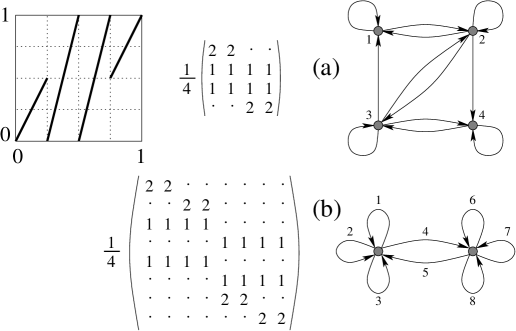
Figure 1: An example of a quantizable map and the corresponding matrices $\mathbf{B}$: (a) $|{\cal M}|=4$, the atoms of the partition are represented by the vertices of the graph; (b) $|{\cal M}|=8$, the atoms of the partition are represented by the edges of the graph.

If we view the interval $[0,1]$ with the uniform measure as a probability space, we can write $B_{jk}=\mathbb{P}\left(S(x)\in E_{k}|x\in E_{j}\right)$.

Lemma 1.

Let the set of endpoints of the partition ${\cal M}$ be invariant under $S$. Then the matrix $\mathbf{B}$ defined by (6) satisfies the following properties:

1. $\mathbf{B}$ is stochastic,

   $$\sum_{k=1}^{M}B_{jk}=1.$$

2. If the atoms $E_{j}$ of the partition ${\cal M}$ have equal measure and the map $S$ preserves this measure then $\mathbf{B}$ is doubly stochastic

   $$\sum_{j=1}^{M}B_{jk}=1.$$

3. If the atoms $E_{j}$ of the partition ${\cal M}$ have equal measure and if the map $S$ is linear with respect to $\mu$ on each atom $E_{j}$ (i.e. $\mu(S(A))=C\mu(A)$ for some $C$ and all $A\in E_{j}$) then

   $$B_{j_{0}j_{1}}B_{j_{1}j_{2}}\cdots B_{j_{k-1}j_{k}}=\frac{\mu\left(\bigcap_{r=0}^{k}S^{-r}\left(E_{j_{r}}\right)\right)}{\mu\left(E_{j_{0}}\right)}.$$ (7)

Proof.

Part 1 follows directly from (6),

$$\sum_{k=1}^{M}B_{jk}=\frac{1}{\mu(E_{j})}\,\,\mu\!\left(E_{j}\cap\left(\bigcup_{k=1}^{M}S^{-1}(E_{k})\right)\right)=\frac{\mu\left(E_{j}\cap[0,1]\right)}{\mu(E_{j})}=1.$$

Part 2 is similar: if $\mu(E_{j})=m$ for all $j$ then

$$\sum_{j=1}^{M}B_{jk}=\frac{1}{m}\,\,\mu\!\left(\left(\bigcup_{j=1}^{M}E_{j}\right)\cap S^{-1}(E_{k})\right)=\frac{\mu\left(S^{-1}(E_{k})\right)}{m}=\frac{\mu(E_{k})}{m}=1.$$

Part 3 is a consequence of the fact that, if $\mu(S(A))=C_{j}\mu(A)$ for all $A\subset E_{j}$, then $B_{jk}$ is either $0$ or $1/C_{j}$. Consider first the case $B_{j_{r}j_{r+1}}=0$ for some $r$. By definition of $\mathbf{B}$, this means that $\mu\left(E_{j_{r}}\cap S^{-1}(E_{j_{r+1}})\right)=0$. Therefore,

$$\mu\left(S^{-r}(E_{j_{r}})\cap S^{-r-1}(E_{j_{r+1}})\right)=0,$$

and the expression on the right hand side of (7) evaluates to zero.

Now consider the case $n=2$ (the case of general $n$ being analogous) with both $B_{j_{0}j_{1}}$ and $B_{j_{1}j_{2}}$ being different from zero. Let, to simplify the notation, $j_{r}=r$. Then

$$B_{0,1}=\frac{\mu\left(E_{0}\cap S^{-1}(E_{1})\right)}{\mu(E_{0})} = \frac{\mu\left(E_{0}\cap S^{-1}(E_{1})\right)}{\mu(E_{1})}$$

$$= \frac{\mu\left(E_{0}\cap S^{-1}\left(E_{1}\cap S^{-1}(E_{2})\right)\right)}{\mu\left(E_{1}\cap S^{-1}(E_{2})\right)},$$

where the last equality is true by virtue of linearity of $S$. Using the definition of $B_{1,2}$ and the identity $S^{-1}\left(A\cap B\right)=S^{-1}\left(A\right)\cap S^{-1}\left(B\right)$, we arrive to

$$B_{0,1}B_{1,2}=\frac{\mu\left(E_{0}\cap S^{-1}(E_{1})\cap S^{-2}(E_{2})\right)}{\mu(E_{1})},$$

which is the sought result, given that $\mu(E_{1})=\mu(E_{0})$. ∎

As mentioned earlier, we are interested in sequences of partitions.

Condition 2.

We consider sequences of partitions ${\cal M}_{n}$ that satisfy

1. the atoms within each of the partition have equal measure;

2. the sets of endpoints ${\cal E}({\cal M}_{n})$ are forward-invariant under the action of $S$;

3. the set of the endpoints of ${\cal M}_{n}$ contains the $j$-th pre-image of the endpoints of ${\cal M}_{0}$ for all $j=1,\ldots n$.

Remark 3.

Given a map $S$ satisfying Condition 1 one can always construct a sequence of partitions satisfying Condition 2.

Remark 4.

Conditions 1(b) and 1(c) imply that the map $S$ is non-contracting, $\mu(S(A))\geq\mu(A)$. If the map is ergodic (see definition 1 in section 4), Condition 1(a) implies that the preimages of ${\cal E}({\cal M}_{0})$ with respect to $S$ are dense in $[0,1]$. This, in turn, implies that the size of the atoms of the partitions ${\cal M}_{n}$ tends to zero (or, equivalently, $M_{n}\to\infty$).

The following lemma explains the way in which such sequences of partitions ‘resolve’ the dynamics.

Lemma 2.

Given a partition ${\cal M}_{n}$ satisfying Condition 2, let $k_{0}$ and $k_{n}$ be such that $S^{n}(E_{k_{0}})\supset E_{k_{n}}$ (cf. Remark 1). Then there exists a unique sequence $k_{1},\ldots,k_{n-1}$ such that

$$x\in E_{k_{0}}\mbox{ and }S^{n}(x)\in E_{k_{n}}\qquad\Rightarrow\qquad S^{j}(x)\in E_{k_{j}}\quad\forall 0\leq j\leq n.$$

Proof.

Consider an atom $E$ of the partition ${\cal M}_{n}$. Condition 2(c) means that for every $j=0,\ldots k$, the image $S^{j}(E)$ lies in a single atom of the “primary” partition ${\cal M}_{0}$. Since the map $S$ is one-to-one on each atom of ${\cal M}_{0}$, we conclude, by induction, that $S^{j}$ is one-to-one on $E$ for every $j=1,\ldots n+1$.

Assume that the statement of the lemma is incorrect: there are two points, $x$ and $y$, that satisfy, without loss of generality, $x,y\in E_{1}$, $S^{r}(x)\in E_{2}$, $S^{r}(y)\in E_{3}$ and $S^{n}(x),S^{n}(y)\in E_{4}$. Remark 1 implies the following inclusions:

$$S^{r}(E_{1})\supset E_{2},\qquad S^{2}(E_{1})\supset E_{3},\qquad S^{n-r}(E_{2})\supset E_{4},\qquad S^{n-r}(E_{3})\supset E_{4}.$$

Thus each $z\in E_{4}$ has $n-r$-preimages in both sets $E_{2}$ and $E_{3}$ and, therefore, two distinct $n$-preimages in $E_{1}$. This contradicts the earlier conclusion that $S^{n}$ is one-to-one on $E_{1}$. ∎

Remark 5.

Obviously, Lemma 2 is valid if, instead of the “position” of $S^{n}(x)$ (i.e. the atom $E_{j}$ such that $S^{n}(x)\in E_{j}$), we know the position of $S^{m}(x)$ for some $m<n$: we can still recover positions of all iterates $S^{j}(x)$ for $0<j<m$. In fact, a careful inspection of the proof reveals that the Lemma would still be true for $m=n+1$. However, if we know only that $x\in E_{1}$ and $S^{n+2}(x)\in E_{2}$, we would not be able to pinpoint $S^{j}(x)$, $0<j<n+2$, to any particular atom of the partition ${\cal M}_{n}$.

The next lemma exhibits the block structure of the matrix $\mathbf{B}$.

Lemma 3.

For a partition ${\cal M}_{n}$, $n>0$, define an equivalence relation between atoms by setting $E_{j}\sim E_{k}$ if $S(E_{j})$ intersects $S(E_{k})$ and then completing by transitivity. Then the maximum number of elements in an equivalence class is uniformly bounded with respect to $n$.

For example, in the partition of Figure 1, part (b), the atoms $E_{1}$, $E_{2}$, $E_{3}$ and $E_{5}$ form one equivalence class and the other four atoms form another equivalence class. Note that, if the atoms of a partition are represented by edges of the graph, the equivalence classes correspond to the groups of edges ending in the same vertex. For the map in Figure 1 the uniform bound on the size of an equivalence class is 4, as will be evident from the proof.

Proof.

Take an atom $A$ of the primary partition ${\cal M}_{0}$ and let $(x_{1},y_{1}),\ldots,(x_{k},y_{k})$ be the disjoint intervals forming the pre-image of $A$ with respect to $S$. By Condition 1(c) these intervals contain no endpoints of ${\cal M}_{0}$, therefore the map $S$ is linear on each interval. Condition 1 also implies that all slopes of the map $S$ are integer. Denote the slope of $S$ on the interval $(x_{j},y_{j})$ by $s_{j}$. To simplify the notation we assume that all $s_{j}$ are positive. Let $p$ be the least common multiple of $s_{j}$.

Condition 2(c) implies that $x_{j}$ and $y_{j}$ are endpoints of the partition ${\cal M}_{n}$. Choose $x_{j}^{\prime}\in{\cal E}({\cal M}_{n})$ such that the interval $(x_{j},x_{j}^{\prime})$ contains exactly $p/s_{j}$ atoms of the partition ${\cal M}_{n}$. Since the atoms of ${\cal M}_{n}$ have equal length (which we denote by $\mu_{n}$),

$$s_{j_{1}}(x_{j_{1}}^{\prime}-x_{j_{1}})=s_{j_{2}}(x_{j_{2}}^{\prime}-x_{j_{2}})=p\mu_{n},\qquad\mbox{for any }j_{1},j_{2}.$$ (8)

Moreover, the selected points $x_{j}^{\prime}$ are the closest to the respective $x_{j}$ to satisfy both condition (8) and $x_{j}^{\prime}\in{\cal E}({\cal M}_{n})$. In particular, this implies that $x_{j}^{\prime}\leq y_{j}$, since setting $x_{j}^{\prime}=y_{j}$ would also satisfy condition (8).

From the above we can conclude that $S$ maps all intervals $(x_{j},x_{j}^{\prime})$ to the same subinterval of $A$. The atoms of ${\cal M}_{n}$ making up the intervals $(x_{j},x_{j}^{\prime})$ thus form an equivalence class of size $p/s_{1}+\cdots+p/s_{k}$, which is independent of $n$.

We can now repeat this procedure with intervals $(x_{1}^{\prime},y_{1}),\ldots,(x_{k}^{\prime},y_{k})$ and, thereafter, with all atoms $A$ of the partition ${\cal M}_{0}$. If some of the slopes $s_{j}$ are negative, the procedure would still go through with minor variations. ∎

Having obtained a sequence of doubly stochastic matrices $\mathbf{B}_{n}$ we define their “quantizations” as unitary matrices $\mathbf{U}_{n}$ such that

$$(\mathbf{B}_{n})_{jk}=\left|(\mathbf{U}_{n})_{jk}\right|^{2}.$$ (9)

The doubly stochastic matrices $\mathbf{B}$ for which finding a corresponding $\mathbf{U}$ is possible are called unistochastic.

Condition 3.

We assume that the map $S$ is such that all of the corresponding matrices $\mathbf{B}_{n}$, bar finitely many, are unistochastic.

Not all bistochastic matrices are unistochastic. However, formulating a general sufficient conditions that ensure unistochasticity is a question of considerable difficulty. The interested reader is referred to [27, 40] and the references therein where some necessary conditions are discussed and where examples of maps satisfying and failing Condition 3 are given. To convince the reader that the class of maps $S$ satisfying Condition 3 is far from empty we state the following sufficient condition.

Lemma 4.

If the slopes of the map $S$ satisfying Condition 1 are all equal (modulo sign), Condition 3 is also satisfied.

Proof.

This Lemma follows simply from the proof of Lemma 3. Indeed, let $s$ be the absolute value of the slope of $S$. Then all matrices $\mathbf{B}_{n}$, $n>0$, have a block structure with blocks of the size $s\times s$ and elements $1/s$. Thus the question is really about finding an $s\times s$ unitary matrix with all elements satisfying $|U_{jk}|^{2}=1/s$. One example of such matrix is the Fourier matrix with elements $U_{jk}=\exp\{2\pi ijk/s\}/\sqrt{s}$. ∎

Example 1.

An example of a map $S$ which has unequal slopes but is still unistochastic is provided by the map of Figure 1.

Remark 6.

An observant reader would notice that, given one unitary $\mathbf{U}$ satisfying (9), one can produce infinitely many such matrices. For example, one can multiply a given $\mathbf{U}$ by an arbitrary diagonal unitary matrix. However, the results of our paper do not depend on the precise choice of matrices $\mathbf{U}_{n}$, provided that condition (9) is satisfied.

One can associate a graph to the matrices $\mathbf{B}$ and $\mathbf{U}$ in the following way: the indices of the matrices enumerate the directed edges of the graph; the end of an edge $j$ coincides with the start of the edge $k$ if the matrix element $B_{jk}$ is non-zero. The number of distinct vertices in such a construction should be maximized, then the vertices will correspond to the equivalence classes of Lemma 3.

The matrix $\mathbf{B}$ defines a Markov chain on the edges of the graph with $B_{jk}$ representing the transition probability from $j$ to $k$. The matrix $\mathbf{U}$ can be viewed as a quantum propagator on the graph. This geometrical interpretation of the two matrices as a graph will be helpful in the later sections when we use trajectories on the graph to describe properties of the eigenvectors of $\mathbf{U}$.

It is also possible to associate vertices of a graph to the indices of $\mathbf{B}$, see Figure 1, part (a). We use directed edges for reasons of tradition, rather than convenience.

4 Quantization of the observables

Having defined the sequences of unitary matrices $\mathbf{U}_{n}$, ergodic properties of whose eigenvectors we are going to study, we need a final ingredient, the observables $\mathbf{O}_{n}$. For a general sequence of graphs, it is not obvious how to define a consistent sequence of observables. In our case, however, there is a natural answer.

We use the discretizations of functions $\phi\in L^{2}[0,1]$ as our observables. Fix a partition ${\cal M}$ (the semi-classical limit corresponds to $|{\cal M}|\to\infty$). If the function $\phi$ is constant on each atom of the partition ${\cal M}$, its quantization $\mathbf{O}=\mathbf{O}(\phi)$ is a diagonal matrix with entries $O_{jj}=\phi(x)$ where $x\in E_{j}$. If $\phi$ is not constant on the atoms of ${\cal M}$, we replace $\phi$ by its local average. More precisely, we introduce the piecewise constant function $\widehat{\phi}$ defined by

$$\widehat{\phi}(x)=\frac{1}{\mu(E_{j})}\int_{E_{j}}\phi(y)d\mu(y),\qquad\mbox{where }E_{j}\ni x.$$

Then we define $\mathbf{O}=\mathbf{O}(\phi)$ as before, by

$$O_{jj}=O_{jj}(\phi)=\widehat{\phi}(E_{j})=\frac{1}{\mu(E_{j})}\int_{E_{j}}\phi(y)d\mu(y).$$ (10)

It is convenient to describe $\widehat{\phi}$ using the notions of probability theory. In probabilistic language, $\phi$ is a random variable defined on the probability space $[0,1]$ and $\widehat{\phi}$ is its conditional expectation, $\widehat{\phi}=\mathbb{E}\left[\left.\phi\right|{\cal M}\right]$. We will also use the notation of expectation to denote the integral over $[0,1]$:

$$\mathbb{E}\phi=\int_{0}^{1}\phi(x)d\mu(x).$$

In particular, $\|\phi\|_{2}=\left(\mathbb{E}\phi^{2}\right)^{1/2}$.

To prove quantum ergodicity, we will rely on the ergodicity of the classical map $S$. Since our observables are in $L^{2}$, the relevant version of the ergodic theorem is the $L^{2}$ ergodic theorem (see, e.g., [41]).

Definition 1.

A map $S:[0,1]\to[0,1]$ is ergodic if any set $A\subset[0,1]$ satisfying

$$S^{-1}(A)=A$$

has either full or zero measure.

Theorem 1.

($L^{2}$ Ergodic Theorem) If $\phi\in L^{2}[0,1]$ and $S$ is ergodic, then

$${\cal V}_{T}(\phi)\stackrel{{\scriptstyle\mathrm{def}}}{{=}}\mathbb{E}\left(\frac{1}{T}\sum_{t=1}^{T}\phi\circ S^{t}-\mathbb{E}\phi\right)^{2}\to 0.$$ (11)

Since the ergodic theorem applies to any function from $\phi\in L^{2}$, it also applies to $\widehat{\phi}$, whatever partition ${\cal M}$ was used to produce it. Unfortunately, a uniform estimate for the rate of convergence in (11) for different hat-versions of the same $\phi$ is not known [42]. However, it is easy to see that, for fixed $T$,

$${\cal V}_{T}(\widehat{\phi})\to{\cal V}_{T}(\phi)$$ (12)

as the partition in the definition of $\widehat{\phi}$ gets finer.

5 Quantum variance of an observable

Given a map $S$ and a sequence of partitions ${\cal M}_{n}$ we have constructed a sequence of Markov matrices $\mathbf{B}_{n}$, which, in turn, give rise to unitary matrices $\mathbf{U}_{n}$. On the other hand we are given an observable $\phi$ and we have constructed a corresponding sequence of diagonal matrices $\mathbf{O}_{n}$, which “quantize” $\phi$. We denote by $M_{n}$ the number of atoms in the partition ${\cal M}_{n}$. This is also the size of the matrices $\mathbf{B}_{n}$, $\mathbf{U}_{n}$ and $\mathbf{O}_{n}$. The semiclassical limit corresponds to $M_{n}\to\infty$.

Let $\boldsymbol{\psi}^{(n)}_{j}$, where $j=1,\ldots,M_{n}$ denote the orthonormal eigenvectors of $\mathbf{U}_{n}$. If an eigenvalue is degenerate, the particular choice of the basis for its eigenspace is unimportant. As discussed earlier, to show quantum ergodicity it is sufficient to prove that

$$\frac{1}{M_{n}}\sum_{j=1}^{M_{n}}\left(\boldsymbol{\psi}^{(n)}_{j},\mathbf{O}_{n}\boldsymbol{\psi}^{(n)}_{j}\right)\to\mathbb{E}(\phi)=\int_{0}^{1}\phi(x)dx$$ (13)

and

$$V_{n}=\frac{1}{M_{n}}\sum_{j=1}^{M_{n}}\left|\left(\boldsymbol{\psi}^{(n)}_{j},\mathbf{O}_{n}\boldsymbol{\psi}^{(n)}_{j}\right)-\mathbb{E}(\phi)\right|^{2}\to 0,$$ (14)

as $n\to\infty$. It is straightforward to verify (13). Indeed, from the unitarity of $\mathbf{U}_{n}$ and the definition of $\mathbf{O}_{n}$,

$$\frac{1}{M_{n}}\sum_{j=1}^{M_{n}}\left(\boldsymbol{\psi}^{(n)}_{j},\mathbf{O}_{n}\boldsymbol{\psi}^{(n)}_{j}\right)=\frac{1}{M_{n}}\operatorname{Tr}\mathbf{O}_{n}=\mathbb{E}\left(\widehat{\phi}\right)=\mathbb{E}(\phi).$$

Thus the main task is to show (14).

Without loss of generality we can assume that $\mathbb{E}(\phi)=0$. In what follows we will omit the sub- and super-scripts $n$ unless we want to underline the dependence of a quantity on $n$ and on the partition ${\cal M}_{n}$.

To obtain an estimate of $V_{n}$ we employ some standard manipulations. If $\boldsymbol{\psi}$ is an eigenvector of a unitary matrix $\mathbf{U}$, we have, for any matrix $\mathbf{O}$ (not necessarily diagonal) and all $t\in\mathbb{N}$

$$\left(\boldsymbol{\psi},\mathbf{O}\boldsymbol{\psi}\right)=\left(\mathbf{U}^{t}\boldsymbol{\psi},\mathbf{O}\mathbf{U}^{t}\boldsymbol{\psi}\right)=\left(\boldsymbol{\psi},(\mathbf{U}^{*})^{t}\mathbf{O}\mathbf{U}^{t}\boldsymbol{\psi}\right).$$

Summing this equality over $t=0,\ldots T-1$ we obtain

$$\left(\boldsymbol{\psi},\mathbf{O}\boldsymbol{\psi}\right)=\left(\boldsymbol{\psi},\frac{1}{T}\sum_{t=0}^{T-1}(\mathbf{U}^{*})^{t}\mathbf{O}\mathbf{U}^{t}\boldsymbol{\psi}\right).$$

We introduce the shorthand $\mathbf{O}_{n,T}$ for the time average of $\mathbf{O}_{n}$,

$$\mathbf{O}_{n,T}=\frac{1}{T}\sum_{t=0}^{T-1}(\mathbf{U}_{n}^{*})^{t}\mathbf{O}_{n}\mathbf{U}_{n}^{t}.$$

Using Cauchy-Schwarz inequality and orthonormality of $\{\boldsymbol{\psi}_{j}\}$ we estimate

$$\left|\left(\boldsymbol{\psi},\mathbf{O}\boldsymbol{\psi}\right)\right|^{2}=\left|\left(\boldsymbol{\psi},\mathbf{O}_{T}\boldsymbol{\psi}\right)\right|^{2}\leq\left(\mathbf{O}_{T}\boldsymbol{\psi},\mathbf{O}_{T}\boldsymbol{\psi}\right)=\left(\boldsymbol{\psi},\mathbf{O}_{T}^{*}\mathbf{O}_{T}\boldsymbol{\psi}\right),$$

and obtain

$$V_{n} = \frac{1}{M_{n}}\sum_{j=1}^{M_{n}}\left|\left(\boldsymbol{\psi}_{j},\mathbf{O}\boldsymbol{\psi}_{j}\right)\right|^{2}$$ (15)

$$\leq \frac{1}{M_{n}}\sum_{j=1}^{M_{n}}\left(\boldsymbol{\psi}_{j},\mathbf{O}_{T}^{*}\mathbf{O}_{T}\boldsymbol{\psi}_{j}\right)=\frac{1}{M_{n}}\operatorname{Tr}\left(\mathbf{O}_{T}^{*}\mathbf{O}_{T}\right)\stackrel{{\scriptstyle\mathrm{def}}}{{=}}K(n,T)$$

It is important to note that the above inequality is valid for all values of $T$. Thus, to show that $V_{n}\to 0$, we are free to choose an appropriate $T=T(n)$ for each $n$ as long as we can demonstrate that

$$K(n,T(n))=\frac{1}{M_{n}}\operatorname{Tr}\left(\mathbf{O}_{n,T(n)}^{*}\mathbf{O}_{n,T(n)}\right)\to 0,$$

as $n\to\infty$. In the following sections we prove that $T(n)=n$ is a suitable choice for this task.

For our purposes, it is more convenient to work with the matrices $\mathbf{S}_{n,T}$ defined by

$$\mathbf{S}_{n,T}=\mathbf{U}_{n}^{T}\mathbf{O}_{n,T}=\frac{1}{T}\sum_{t=0}^{T-1}\mathbf{U}_{n}^{T-t}\mathbf{O}_{n}\mathbf{U}_{n}^{t},$$

which is equivalent to working with $\mathbf{O}_{T}$ since $\mathbf{S}^{*}_{T}\mathbf{S}_{T}=(\mathbf{U}^{T}\mathbf{O}_{T})^{*}(\mathbf{U}^{T}\mathbf{O}_{T})=\mathbf{O}_{T}^{*}\mathbf{O}_{T}$.

Multiplying $\mathbf{S}_{T}^{*}\mathbf{S}$ out we obtain

$$\frac{1}{M}\operatorname{Tr}\left(\mathbf{S}_{T}^{*}\mathbf{S}_{T}\right)=\frac{1}{M}\sum_{s,f=1}^{M}|(\mathbf{S}_{T})_{s,f}|^{2}.$$

We can expand the entries of $\mathbf{S}_{T}$ in terms of trajectories on the graph. Using the definition of $\mathbf{S}_{T}$, we obtain

$$(\mathbf{S}_{T})_{sf} = \frac{1}{T}\sum_{t=0}^{T-1}\sum_{b_{0},\ldots b_{T}}U_{b_{0},b_{1}}\cdots U_{b_{T-t-1},b_{T-t}}O_{b_{T-t},b_{T-t}}\cdots U_{b_{T-1},b_{T}}$$

$$= \sum_{b_{0},\ldots b_{T}}U_{b_{0},b_{1}}\cdots U_{b_{T-1},b_{T}}\left(\frac{1}{T}\sum_{t=0}^{T-1}O_{b_{T-t},b_{T-t}}\right),$$

where the inner sum in the first line is over all sequences of bonds satisfying $b_{0}=s$ and $b_{T}=f$. Such a sequence of bonds we will call a trajectory. Only trajectories compatible with the graph’s geometry (i.e. those for which $U_{b_{j}b_{j+1}}\neq 0$) contribute to $K(n,T)$. A trajectory $\tau=(b_{0},\ldots,b_{T})$ is said to have length $T$ and amplitude

$$A_{\tau}\stackrel{{\scriptstyle\mathrm{def}}}{{=}}U_{b_{0}b_{1}}\cdots U_{b_{T-1}b_{T}}.$$

We will denote by $\Phi_{\tau}$ the average of the observable over the trajectory $\tau$,

$$\Phi_{\tau}\stackrel{{\scriptstyle\mathrm{def}}}{{=}}\frac{1}{T}\left(O_{b_{1}b_{1}}+\ldots+O_{b_{T}b_{T}}\right).$$

To summarize, we have shown that

$$V_{n}\leq K(n,T)=\frac{1}{M_{n}}\operatorname{Tr}\left(\mathbf{S}_{T}^{*}\mathbf{S}_{T}\right)=\frac{1}{M_{n}}\sum_{s,f=1}^{M_{n}}\left|\sum_{\tau:s\to f}\Phi_{\tau}A_{\tau}\right|^{2}\\ =\frac{1}{M_{n}}\sum_{s,f=1}^{M_{n}}\sum_{\tau_{1},\tau_{2}:s\to f}\Phi_{\tau_{1}}^{*}\Phi_{\tau_{2}}A^{*}_{\tau_{1}}A_{\tau_{2}}.$$ (16)

where the inner sum is over all possible trajectories of length $T$ starting at $s$ and finishing at $f$.

6 Diagonal terms

Equation (16) is reminiscent of a trace formula expansion of the spectral form factor (i.e. of the Fourier transform of the spectral two-point correlation function), in particular of a graph, see e.g. [14]. Such expansions are notoriously difficult to analyze rigorously as both $T$ and the size of the graph increase. The starting point of any such analysis is the evaluation of the contribution from the diagonal terms, obtained by restricting the last sum in (16) to identical trajectories, $\tau_{1}=\tau_{2}$. It is usually assumed that the off-diagonal terms sum up to a subdominant contribution, when $T$ and the size of the graph scale appropriately. This idea, called the diagonal approximation was first introduced for a general class of systems in [43]. On graphs it was explored, in particular, in [14, 44]. It is difficult, however, to give an a priori estimate on the size of the off-diagonal contributions and the analysis is usually restricted to evaluating the contributions coming from specific classes of interacting trajectories [15, 16, 17, 18].

Our strategy now is to calculate the contribution from the diagonal terms in (16). Then we will show that, in the case of graphs constructed from 1d maps, we can actually estimate the off-diagonal terms by virtue of being able to choose an appropriate $T=T(n)$.

To evaluate the diagonal contribution

$$K^{\mathrm{(diag)}}(n,T)\stackrel{{\scriptstyle\mathrm{def}}}{{=}}\frac{1}{M_{n}}\sum_{\tau}\left|\Phi_{\tau}\right|^{2}\left|A_{\tau}\right|^{2},$$

we make two observations. First, by the definition of the amplitude $A_{\tau}$ and the defining property of the matrix $\mathbf{U}$, equation (9), we obtain

$$\left|A_{\tau}\right|^{2}=|U_{b_{0},b_{1}}|^{2}\cdots|U_{b_{T-1},b_{T}}|^{2}=B_{b_{0},b_{1}}\cdots B_{b_{T-1},b_{T}}.$$

Now we recall Lemma 1, part 3, and conclude that

$$\left|A_{\tau}\right|^{2}=\frac{\mu\left(\bigcap_{t=0}^{T}S^{-t}(E_{b_{t}})\right)}{\mu\left(E_{b_{0}}\right)}.$$

On the other hand, by definition of $\Phi_{\tau}$,

$$\Phi_{\tau}=\frac{1}{T}\sum_{t=1}^{T}O_{b_{t},b_{t}}=\frac{1}{T}\sum_{t=1}^{T}\widehat{\phi}(E_{b_{t}})=\frac{1}{T}\sum_{t=1}^{T}\widehat{\phi}\circ S^{t}\left(S^{-t}(E_{b_{t}})\right),$$

where $\widehat{\phi}(E_{b})$ denotes the (constant) value of the function $\widehat{\phi}$ on the atom $E_{b}$. In fact, it is easy to see that $\Phi_{\tau}$ coincides with the value of the function

$$\widehat{\phi}_{T}\stackrel{{\scriptstyle\mathrm{def}}}{{=}}\frac{1}{T}\sum_{t=1}^{T}\widehat{\phi}\circ S^{t}$$

on the set $\bigcap_{t=0}^{T}S^{-t}(E_{b_{t}})\stackrel{{\scriptstyle\mathrm{def}}}{{=}}E_{b_{0},\ldots,b_{T}}$, if this set is non-empty. If it is empty, the value of $\Phi_{\tau}$ is of no consequence since the trajectory $\tau$ is then incompatible with the graph’s geometry and $A_{\tau}=0$.

The measure of all atoms $E_{b}$ is assumed to be equal. More precisely, it is equal to $1/M_{n}$, since $M_{n}$ is the total number of the atoms. Collecting our observations together, we can express the diagonal term as

$$K^{\mathrm{(diag)}}(n,T) = \frac{1}{M_{n}}\sum_{\tau}\left(\widehat{\phi}_{T}\left(E_{b_{0},\ldots,b_{T}}\right)\right)^{2}\frac{\mu(E_{b_{0},\ldots,b_{T}})}{M_{n}^{-1}}$$

$$= \int_{0}^{1}\left(\widehat{\phi}_{T}(x)\right)^{2}dx=\mathbb{E}\left(\frac{1}{T}\sum_{t=1}^{T}\widehat{\phi}\circ S^{t}\right)^{2}={\cal V}_{T}(\widehat{\phi}).$$

Thus, by the $L^{2}$ ergodic theorem (Theorem 1), $K^{\mathrm{(diag)}}(n,T)$ goes to zero as $T\to\infty$. On the other hand, $K(n,T)$ is bounded below by a non-negative $V_{n}$ which is, generically, non-zero for a fixed $n$. This shows that the diagonal term is a poor approximation to $K(n,T)$ in the limit $T\to\infty$. Luckily, this is not the limit we have to take.

7 Completion of the proof of quantum ergodicity

Lemma 2 has a very important consequence for the inner sum in (16).

Lemma 5.

The diagonal term $K^{\mathrm{(diag)}}(n,T)$ gives the exact value of $K(n,T)$ up to time $T=n$, i.e.

$$K(n,T)=K^{\mathrm{(diag)}}(n,T)={\cal V}_{T}(\widehat{\phi})\qquad\mbox{if }T\leq n,$$

where $\widehat{\phi}=\mathbb{E}\left[\left.\phi\right|{\cal M}_{n}\right]$.

Proof.

By Lemma 2, for every pair of bonds $s$ and $f$, there is at most one trajectory going from $s$ to $f$ in $T\leq n$ steps. Thus, for $T\leq n$,

$$K(n,T)=\frac{1}{M_{n}}\sum_{s,f=1}^{M_{n}}\left|\sum_{\tau:s\to f}\Phi_{\tau}A_{\tau}\right|^{2}\\ =\frac{1}{M_{n}}\sum_{s,f=1}^{M_{n}}\left|\Phi_{\tau(s\to f)}A_{\tau(s\to f)}\right|^{2}=\frac{1}{M_{n}}\sum_{\tau}\left|\Phi_{\tau}A_{\tau}\right|^{2}=K^{\mathrm{(diag)}}(n,T).$$

∎

As a consequence, we have the following result.

Theorem 2.

(Quantum Ergodicity) Let the map $S$ and the sequence of partitions $\{{\cal M}_{n}\}$ satisfy Conditions 1, 2 and 3; let $\{\mathbf{U}_{n}\}$ be the corresponding sequence of unitary matrices with eigenvectors $\boldsymbol{\psi}^{(n)}_{j}$; and let $\{\mathbf{O}_{n}\}$ be a sequence of diagonal matrices corresponding to an observable $\phi\in L^{2}[0,1]$ with $\mathbb{E}\phi=0$. If $S$ is ergodic, then

$$V_{n}=\frac{1}{M_{n}}\sum_{j=1}^{M_{n}}\left|\left(\boldsymbol{\psi}^{(n)}_{j},\mathbf{O}_{n}\boldsymbol{\psi}^{(n)}_{j}\right)\right|^{2}\to 0\qquad\mbox{as }n\to\infty.$$

Proof.

The variance $V_{n}$ is majorized by $K(n,T)$ for any $T$. We combine Lemma 5 with equation (12) we conclude that, for a fixed $T$,

$$K(n,T)\to{\cal V}_{T}(\phi)\qquad\mbox{as }n\to\infty.$$

Now we use the standard $\varepsilon/2$ argument: for any $\varepsilon>0$, by Theorem 1 we can find $T$ such that ${\cal V}_{T}(\phi)<\varepsilon/2$. Having fixed this $T$, we find $n(\varepsilon,T)$ such that $|K(n,T)-{\cal V}_{T}(\phi)|<\varepsilon/2$ for all $n\geq n(\varepsilon,T)$. Combining the above,

$$V_{n}\leq K(n,T)<\varepsilon/2+\varepsilon/2$$

as long as $n\geq n(\varepsilon,T)$. Since $\varepsilon$ was arbitrary, we conclude that $V_{n}\to 0$. ∎

Remark 7.

One can avoid the $\varepsilon/2$ argument in the following way. Taking the limit $n\to\infty$ of the inequality $V_{n}\leq K(n,T)$ produces

$$0\leq\limsup_{n\to\infty}V_{n}\leq\limsup_{n\to\infty}K(n,T)={\cal V}_{T}(\phi).$$

Now taking the $T\to\infty$ limit, we obtain

$$0\leq\limsup_{n\to\infty}V_{n}=\limsup_{T\to\infty}\limsup_{n\to\infty}V_{n}\leq\limsup_{T\to\infty}{\cal V}_{T}(\phi)=0.$$

8 Egorov property

In Section 4 we defined a procedure to obtain a piecewise constant function $\widehat{\phi}$ given a function $\phi\in L^{2}[0,1]$. It is enlightening to see how $\widehat{\phi\circ S}$ is related to $\widehat{\phi}$.

By definition,

$$\widehat{\phi\circ S}\Big{|}_{E_{j}}=\frac{1}{\mu(E_{j})}\int_{E_{j}}\phi(S(y))d\mu(y)=\frac{1}{\mu(E_{j})}\int_{S(E_{j})}\phi(z)\frac{d\mu(z)}{|S^{\prime}(y)|}.$$

Since $S$ is linear on $E_{j}$, its derivative is constant. In fact, it is easy to see that $1/|S^{\prime}(y)|=B_{jk}$, where $y\in E_{j}$ and $S(y)\in E_{k}$. Thus we have

$$\widehat{\phi\circ S}\Big{|}_{E_{j}}=\sum_{k:E_{k}\cap S(E_{j})\neq\emptyset}B_{jk}\frac{1}{\mu(E_{j})}\int_{E_{k}}\phi(z)d\mu(z),$$

where the sum is over the decomposition of the set $S(E_{j})$ into atoms $E_{k}$. Since $B_{jk}=0$ whenever $E_{k}\cap S(E_{j})$ is empty and since $\mu(E_{j})$ is independent of $j$, we arrive to the following conclusion

Lemma 6.

If, for a given partition ${\cal M}$, the matrices $\mathbf{B}$, $\mathbf{O}(\phi)$ and $\mathbf{O}(\phi\circ S)$ are defined according to (6) and (10) then

$$O_{jj}(\phi\circ S)=\sum_{k=1}^{M}B_{jk}O_{kk}(\phi),$$

where $M$ is the number of atoms in the partition ${\cal M}$.

Lemma 6 is a rather beautiful manifestation of the inter-consistency between the discretization procedures for maps $S$ and observables $\phi\in L^{2}$. Namely, the discretization commutes with the action of $S$ on $L^{2}$. In this, Lemma 6 is a classical analogue of the Egorov property, a result which shows that the unitary matrices $\mathbf{U}_{n}$ faithfully represent the action of the classical map $S$.

Theorem 3.

(Egorov property) Let the map $S$ and the sequence of partitions $\{{\cal M}_{n}\}$ satisfy Conditions 1, 2 and 3; let $\{\mathbf{U}_{n}\}$ be the corresponding sequence of unitary matrices with eigenvectors $\boldsymbol{\psi}^{(n)}_{j}$; and let $\{\mathbf{O}_{n}\}$ be a sequence of diagonal matrices corresponding to an observable $\phi$. If $\phi$ is Lipschitz continuous then

$$\|\mathbf{U}_{n}\mathbf{O}_{n}(\phi)\mathbf{U}_{n}^{-1}-\mathbf{O}_{n}(\phi\circ S)\|=O({M_{n}}^{-1}),$$

where the norm is the operator norm on the Euclidean space $\mathbb{R}^{M_{n}}$.

Proof.

We fix the partition ${\cal M}_{n}$, denote the corresponding $\mathbf{U}\mathbf{O}\mathbf{U}^{-1}$ by $\mathbf{Q}$ and observe that, while $\mathbf{O}(\phi\circ S)$ is a diagonal matrix, $\mathbf{Q}$ is not necessarily so.

First we treat the diagonal elements of $\mathbf{Q}$. Writing them out explicitly we get

$$Q_{jj}=\sum_{r=1}^{M_{n}}U_{jr}O_{rr}U^{-1}_{rj}=\sum_{r=1}^{M_{n}}U_{jr}O_{rr}\overline{U_{jr}}=\sum_{r=1}^{M_{n}}|U_{jr}|^{2}O_{rr}=O_{jj}(\phi\circ S),$$

where we used the unitarity of $\mathbf{U}$ and its defining property, $|U_{jr}|^{2}=B_{jr}$ and Lemma 6.

For the off-diagonal elements of $\mathbf{Q}$ we have

$$Q_{jk}=\sum_{r=0}^{M_{n}}U_{jr}O_{rr}U^{-1}_{rk} = \sum_{r=0}^{M_{n}}U_{jr}(O_{rr}-C)\overline{U_{kr}}+C\sum_{r=0}^{M_{n}}U_{jr}\overline{U_{kr}}$$

$$= \sum_{r=0}^{M_{n}}U_{jr}(O_{rr}-C)\overline{U_{kr}},$$

where $C$ is any constant and we have used the unitarity of $\mathbf{U}$ to conclude that the second sum is zero. We estimate, using Cauchy-Schwarz,

$$|Q_{jk}| \leq \max_{r}|O_{rr}-C|\sum_{r=0}^{M_{n}}|U_{jr}\overline{U_{kr}}|$$

$$\leq \max_{r}|O_{rr}-C|=\max_{x\in S(E_{j})\cap S(E_{k})}|\widehat{\phi}(x)-C|.$$

If $\phi$ is Lipschitz continuous with

$$\|\phi\|_{\mathrm{Lip}}\stackrel{{\scriptstyle\mathrm{def}}}{{=}}\sup_{x\neq y}\frac{|\phi(x)-\phi(y)|}{\mu(x,y)}<\infty,$$

we can estimate further, by choosing appropriate $C$,

$$|Q_{jk}|\leq\frac{1}{2}\big{\|}\widehat{\phi}\big{\|}_{\mathrm{Lip}}\mu\big{(}S(E_{j})\cap S(E_{k})\big{)}\leq\frac{1}{2}\|\phi\|_{\mathrm{Lip}}\max|S^{\prime}(x)|\mu(E_{j})\propto\frac{\|\phi\|_{\mathrm{Lip}}}{M_{n}}.$$

Since $U_{jr}$ is non-zero only if $S(E_{j})\cap E_{r}\neq\emptyset$ and $U_{kr}$ is non-zero only if $S(E_{k})\cap E_{r}\neq\emptyset$, we conclude that $Q_{jk}=0$ if $S(E_{j})$ and $S(E_{k})$ are disjoint. Thus the matrix $\mathbf{Q}$ is of block-diagonal structure, each block corresponding to an equivalence class as defined by Lemma 3. The norm of $\mathbf{Q}-\mathbf{O}(\phi\circ S)$ is equal to the maximum of the norms of the blocks. A norm of a block, in turn, is bounded by its dimension times the maximum absolute value of the element of the block. The dimension of a block is uniformly bounded by Lemma 3. Thus we get

$$\|\mathbf{Q}-\mathbf{O}(\phi\circ S)\|\leq D(S)\frac{\|\phi\|_{\mathrm{Lip}}}{M_{n}}$$

for some constant $D(S)$ which is independent of $\phi$ and $n$. ∎

Remark 8.

If the function $\phi$ is only assumed to be continuous on $[0,1]$, one can prove a weaker property:

$$\|\mathbf{U}_{n}\mathbf{O}_{n}(\phi)\mathbf{U}_{n}^{-1}-\mathbf{O}_{n}(\phi\circ S)\|\to 0\qquad\mbox{as }M_{n}\to\infty.$$

9 Discussion

We have succeeded in proving quantum ergodicity (QE) for a special class of sequences of quantum graphs. However, we would like to mention that the result is expected to hold for much broader class of graphs.

It is true that, given a finite quantum graph $G$, one can associate a 1d map to it by reversing the process described in the paper. Thereafter, it is possible to produce a sequence of graphs, one of which will coincide with the original graph $G$, and answer the question of QE for this sequence. In this sense, each graph corresponds to a 1d map. However, this is not true for every sequence of graphs. In fact, it is not true for most sequences. Examples of such sequences include star graphs with Kirchhoff conditions at the central vertex (for which the question of QE has been answered negatively), the complete (Kirchhoff) graphs, and the star graphs with Fourier central vertex [44], for both of which the QE is expected (but is not known) to hold in some form.

It is reassuring that the proof of QE in the present article suggests a direction for possible generalizations: study the diagonal terms and then find an estimate for the off-diagonal ones. However, for the sequences of graphs described above the diagonal approximation ceases to be exact for $T>1$ (cf. Lemma 5). This makes estimation of the off-diagonal terms a much more difficult task.

Another interesting question to consider is whether quantum unique ergodicity (when the convergence in (1) happens along all sequences of eigenvectors) is true for any quantum graphs. This has been answered in the negative [26] for graphs with Kirchhoff vertices but is unclear for other types if graphs.

Appendix A Connection between variances $V^{S}$ and $V^{U}$

To demonstrate relation (5) we start with summarizing the notation introduced in Section 2. Let the unitary $B\times B$ matrix $\mathbf{S}$ be defined by $\mathbf{S}=\mathbf{S}(\lambda)=e^{i\lambda\mathbf{L}}\mathbf{S}(0)$, where $\mathbf{L}$ is the diagonal matrix of the bond lengths of the graph and $\mathbf{S}(0)$ is some fixed unitary matrix. Let $\{\lambda_{n}\}$ be the (real) solutions of the equation $\det(\mathbf{I}-\mathbf{S}(\lambda))=0$. We assume that the spectrum $\{\lambda_{n}\}$ is non-degenerate, which is a generic situation [45].

Denote by $\boldsymbol{\phi}_{n}$ the normalized eigenvector of $\mathbf{S}(\lambda_{n})$ corresponding to the eigenvalue 1. By $\boldsymbol{\psi}_{k}(\lambda)$ we denote the $k$-th normalized eigenvector of $\mathbf{S}(\lambda)$. We further denote by $e^{i\theta_{k}(\lambda)}$ the eigenvalues of $\mathbf{S}(\lambda)$, with $\theta_{k}$ chosen to be continuous (indeed smooth) functions of $\lambda$.

When $\lambda=\lambda_{n}$ there is an index $k$ for which $\theta_{k}(\lambda)=0\mod 2\pi$. For this index $k$ we also have $\boldsymbol{\phi}_{n}=\boldsymbol{\psi}_{k}(\lambda)$.

Let $\mathbf{A}$ be a self-adjoint matrix (a generalization of the observable $\mathbf{O}$) with trace 0 (without loss of generality). We are interested in the relationship between two variances,

$$V^{S}(\Lambda,B)=\frac{1}{\overline{N}(\Lambda)}\sum_{\lambda_{n}\leq\Lambda}\langle\boldsymbol{\phi}_{n}|\mathbf{A}|\boldsymbol{\phi}_{n}\rangle^{2},$$

and

$$V^{U}(\mathbf{S}(\lambda),B)=\frac{1}{B}\sum_{k=1}^{B}\langle\boldsymbol{\psi}_{k}(\lambda)|\mathbf{A}|\boldsymbol{\psi}_{k}(\lambda)\rangle^{2},$$

where $\overline{N}(\Lambda)=\Lambda\operatorname{Tr}\mathbf{L}/2\pi$ is the mean number of the eigenvalues $\lambda_{n}$ in the interval $[0,\Lambda]$.

Introducing the notation

$$A_{k}=A_{k}(\lambda)=\left(\boldsymbol{\psi}_{k}(\lambda),\mathbf{A}\boldsymbol{\psi}_{k}(\lambda)\right)$$

we observe that

$$\operatorname{Tr}\mathbf{A}\mathbf{S}^{m}(\lambda)=\sum_{k=1}^{B}A_{k}e^{im\theta_{k}(\lambda)}.$$ (17)

In particular, $\operatorname{Tr}\mathbf{A}=\sum_{k=1}^{B}A_{k}=0$. From the theory of distributions we know that

$$\Delta_{\varepsilon}(\theta)\stackrel{{\scriptstyle\mathrm{def}}}{{=}}\frac{1}{2\pi}\left(1+\sum_{m=1}^{\infty}e^{-m\varepsilon}\left(e^{im\theta}+e^{-im\theta}\right)\right)$$

converges, in the limit $\varepsilon\to 0$, to

$$\Delta(\theta)\stackrel{{\scriptstyle\mathrm{def}}}{{=}}\sum_{r=-\infty}^{\infty}\delta(\theta-2\pi r),$$

where $\delta$ is the Dirac delta function. Substituting in the above identity $\theta=\theta_{k}$, multiplying by $A_{k}$ and performing the summation over $k$ yields

$$\sum_{k=1}^{B}\Delta_{\varepsilon}(\theta_{k})A_{k}=\frac{1}{2\pi}\left(\sum_{m=1}^{\infty}e^{-m\varepsilon}\left(\operatorname{Tr}\mathbf{A}\mathbf{S}^{m}+\operatorname{Tr}\mathbf{A}\mathbf{S}^{-m}\right)\right).$$ (18)

As $\varepsilon\to 0$ this converges to

$$\sum_{k=1}^{B}\Delta(\theta_{k})A_{k}=\sum_{n=1}^{\infty}\frac{A_{k}(\lambda_{n})}{|\theta_{k}^{\prime}(\lambda_{n})|}\delta(\lambda-\lambda_{n}),$$

where, given $\lambda_{n}$, $k$ is chosen to satisfy $\theta_{k}=0$. It is shown in [14] that

$$\theta_{k}^{\prime}(\lambda_{n})=\left(\boldsymbol{\phi}_{n},\mathbf{L}\boldsymbol{\phi}_{n}\right)=\big{(}\boldsymbol{\psi}_{k}(\lambda_{n}),\mathbf{L}\boldsymbol{\psi}_{k}(\lambda_{n})\big{)}\stackrel{{\scriptstyle\mathrm{def}}}{{=}}L_{k}(\lambda_{n}).$$

Clearly, $\theta_{k}^{\prime}(\lambda_{n})>0$ and so we can drop the modulus around $\theta_{k}^{\prime}(\lambda_{n})$ in the previous equation. Now we need the following properties of the approximants to the Dirac delta function,

$$2\pi\lim_{\varepsilon\to 0}\varepsilon\Delta_{\varepsilon}^{2}(x)=\Delta(x)$$

and, if $x_{1}\neq x_{2}$,

$$2\pi\lim_{\varepsilon\to 0}\varepsilon\left(\Delta_{\varepsilon}(x-x_{1})+\Delta_{\varepsilon}(x-x_{2})\right)^{2}=\Delta(x-x_{1})+\Delta(x-x_{2}).$$

Applying these identities gives

$$2\pi\lim_{\varepsilon\to 0}\varepsilon\left(\sum_{k=1}^{B}\Delta_{\varepsilon}(\theta_{k})A_{k}\right)^{2}=\sum_{k=1}^{B}\Delta(\theta_{k})A_{k}^{2}=\sum_{n=1}^{\infty}\frac{A_{k}^{2}(\lambda_{n})}{L_{k}(\lambda_{n})}\delta(\lambda-\lambda_{n}).$$

Integrating the right-hand side with respect to $\lambda$ we get

$$\frac{1}{\overline{N}(\Lambda)}\int_{0}^{\Lambda}\left(\sum_{n=1}^{\infty}\frac{A_{k}^{2}(\lambda_{n})}{L_{k}(\lambda_{n})}\delta(\lambda-\lambda_{n})\right)d\lambda=\frac{1}{\overline{N}(\Lambda)}\sum_{\lambda_{n}<\Lambda}\frac{A_{k}^{2}(\lambda_{n})}{L_{k}(\lambda_{n})}\stackrel{{\scriptstyle\mathrm{def}}}{{=}}\widehat{V}^{S}(\Lambda,B)$$

We will use this quantity to approximate $V^{S}(\Lambda,B)$. It is a good approximation if the bond lengths of the graph are approximately 1 (i.e. the matrix $\mathbf{L}$ is approximately unity):

$$L_{\min}\widehat{V}^{S}(\Lambda,B)\leq V^{S}(\Lambda,B)\leq L_{\max}\widehat{V}^{S}(\Lambda,B),$$

where $L_{\max}$ and $L_{\min}$ are the maximal and minimal bond lengths.

Using (18) and expanding the square we obtain

$$\widehat{V}^{S}(\Lambda,B) = \frac{1}{\overline{N}(\Lambda)}\int_{0}^{\Lambda}2\pi\lim_{\varepsilon\to 0}\varepsilon\left(\sum_{k=1}^{B}\Delta_{\varepsilon}(\theta_{k})A_{k}\right)^{2}d\lambda$$

$$= \frac{1}{2\pi\overline{N}(\Lambda)}\int_{0}^{\Lambda}\lim_{\varepsilon\to 0}\varepsilon\!\!\!\sum_{m_{1},m_{2}=-\infty}^{\infty}\!\!e^{-\varepsilon(|m_{1}|+|m_{2}|)}\operatorname{Tr}\mathbf{A}\mathbf{S}^{m_{1}}\operatorname{Tr}\mathbf{A}\mathbf{S}^{m_{2}}d\lambda.$$

We now take the $\Lambda\to\infty$ limit of the above expression and interchange it with the $\varepsilon$-limit. Due to the rational independence of the bond lengths, the limit

$$\lim_{\Lambda\to\infty}\frac{1}{\overline{N}(\Lambda)}\int_{0}^{\Lambda}\operatorname{Tr}\mathbf{A}\mathbf{S}^{m_{1}}\operatorname{Tr}\mathbf{A}\mathbf{S}^{m_{2}}d\lambda$$

is zero whenever $m_{1}\neq-m_{2}$. Indeed, we recall that $\mathbf{S}=\mathbf{S}(\lambda)=e^{i\lambda\mathbf{L}}\mathbf{S}(0)$ and expand the trace

$$\operatorname{Tr}\mathbf{A}\mathbf{S}^{m}=\sum_{b_{0},\ldots,b_{m}}A_{b_{0},b_{1}}S(0)_{b_{1},b_{2}}\cdots S(0)_{b_{m},b_{0}}\exp(i\lambda L_{p}),$$

where $L_{p}=L_{b_{1}}+\cdots+L_{b_{m}}$. If $L_{p}$ is a sum of $m_{1}$ terms and $L_{q}$ is a sum of $m_{2}\neq m_{1}$ terms, they cannot be equal. Thus, the only case when the phase factors $\exp(i\lambda L_{p})$ in a product of two traces can cancel each other is when $m_{1}=-m_{2}$.

We arrive at

$$\lim_{\Lambda\to\infty}\widehat{V}^{S}(\Lambda,B) = \lim_{\Lambda\to\infty}\frac{1}{\pi\overline{N}(\Lambda)}\int_{0}^{\Lambda}\lim_{\varepsilon\rightarrow 0}\varepsilon\sum_{m=1}^{\infty}e^{-2m\varepsilon}\operatorname{Tr}\mathbf{A}\mathbf{S}^{m}\operatorname{Tr}\mathbf{A}\mathbf{S}^{-m}\,d\lambda$$

$$= \lim_{\Lambda\to\infty}\frac{1}{2\pi\overline{N}(\Lambda)}\int_{0}^{\Lambda}\sum_{k=1}^{B}A_{k}^{2}(\lambda)\,d\lambda$$

$$= \lim_{\Lambda\to\infty}\frac{1}{2\pi\overline{N}(\Lambda)}\int_{0}^{\Lambda}V^{U}(\mathbf{S}(\lambda),B)\,d\lambda.$$

Here we used expansion (17) and the fact that

$$\lim_{\varepsilon\rightarrow 0}\varepsilon\sum_{m=1}^{\infty}e^{-2m\varepsilon}e^{im(\theta_{k_{1}}-\theta_{k_{2}})}=\lim_{\varepsilon\rightarrow 0}\frac{\varepsilon}{e^{2\varepsilon-i(\theta_{k_{1}}-\theta_{k_{2}})}-1}$$

is $1/2$ when $\theta_{k_{1}}=\theta_{k_{2}}$ and 0 otherwise.

References

- [1] A. I. Shnirelman, “Ergodic properties of eigenfunctions,” Uspehi Mat. Nauk, vol. 29, no. 6(180), pp. 181–182, 1974.
- [2] Y. Colin de Verdière, “Ergodicité et fonctions propres du laplacien,” Comm. Math. Phys., vol. 102, no. 3, pp. 497–502, 1985.
- [3] B. Helffer, A. Martinez, and D. Robert, “Ergodicité et limite semi-classique,” Comm. Math. Phys., vol. 109, no. 2, pp. 313–326, 1987.
- [4] S. Zelditch, “Uniform distribution of eigenfunctions on compact hyperbolic surfaces,” Duke Math. J., vol. 55, no. 4, pp. 919–941, 1987.
- [5] P. Gérard and É. Leichtnam, “Ergodic properties of eigenfunctions for the Dirichlet problem,” Duke Math. J., vol. 71, no. 2, pp. 559–607, 1993.
- [6] M. Degli Esposti, S. Graffi, and S. Isola, “Classical limit of the quantized hyperbolic toral automorphisms,” Comm. Math. Phys., vol. 167, no. 3, pp. 471–507, 1995.
- [7] A. Bouzouina and S. De Bièvre, “Equipartition of the eigenfunctions of quantized ergodic maps on the torus,” Comm. Math. Phys., vol. 178, no. 1, pp. 83–105, 1996.
- [8] P. Kurlberg and Z. Rudnick, “Hecke theory and equidistribution for the quantization of linear maps of the torus,” Duke Math. J., vol. 103, no. 1, pp. 47–77, 2000.
- [9] P. Kurlberg and Z. Rudnick, “On quantum ergodicity for linear maps of the torus,” Comm. Math. Phys., vol. 222, no. 1, pp. 201–227, 2001.
- [10] M. Degli Esposti, S. Nonnenmacher, and B. Winn, “Quantum variance and ergodicity for the baker’s map,” Commun. Math. Phys., vol. 263, pp. 325–352, 2006.
- [11] S. De Bièvre, “Quantum chaos: a brief first visit,” in Second Summer School in Analysis and Mathematical Physics (Cuernavaca, 2000), vol. 289 of Contemp. Math., pp. 161–218, Providence, RI: Amer. Math. Soc., 2001.
- [12] G. Berkolaiko, R. Carlson, S. Fulling, and P. Kuchment, eds., Proceedings of Joint Summer Research Conference on Quantum Graphs and Their Applications, 2005. Contemporary Mathematics, AMS, 2006.
- [13] T. Kottos and U. Smilansky, “Quantum chaos on graphs,” Phys. Rev. Lett., vol. 79, pp. 4794–4797, 1997.
- [14] T. Kottos and U. Smilansky, “Periodic orbit theory and spectral statistics for quantum graphs,” Ann. Phys., vol. 274, pp. 76–124, 1999.
- [15] G. Berkolaiko, H. Schanz, and R. S. Whitney, “Leading off-diagonal correction to the form factor of large graphs,” Phys. Rev. Lett., vol. 88, no. 10, p. 104101, 2002.
- [16] G. Berkolaiko, H. Schanz, and R. S. Whitney, “Form factor for a family of quantum graphs: an expansion to third order,” J. Phys. A, vol. 36, no. 31, pp. 8373–8392, 2003.
- [17] G. Berkolaiko, “Form factor for large quantum graphs: evaluating orbits with time reversal,” Waves Random Media, vol. 14, no. 1, pp. S7–S27, 2004.
- [18] G. Berkolaiko, “Correlations within the spectrum of a large quantum graph: a diagrammatic approach,” in Proceedings of Joint Summer Research Conference on Quantum Graphs and Their Applications, 2005 (G. Berkolaiko, R. Carlson, S. Fulling, and P. Kuchment, eds.), AMS, 2006.
- [19] S. Gnutzmann and A. Altland, “Universal spectral statistics in quantum graphs,” Phys. Rev. Lett., vol. 93, no. 19, p. 194101, 2004.
- [20] S. Gnutzmann and A. Altland, “Spectral correlations of individual quantum graphs,” Phys. Rev. E, vol. 72, no. 5, p. 056215, 2005.
- [21] G. Berkolaiko, J. P. Keating, and B. Winn, “Intermediate wave-function statistics,” Phys. Rev. Lett., vol. 91, 2003.
- [22] G. Berkolaiko, J. P. Keating, and B. Winn, “No quantum ergodicity for star graphs,” Comm. Math. Phys., vol. 250, no. 2, pp. 259–285, 2004.
- [23] J. Keating, “Fluctuation statistics for quantum star graphs,” in Proceedings of Joint Summer Research Conference on Quantum Graphs and Their Applications, 2005 (G. Berkolaiko, R. Carlson, S. Fulling, and P. Kuchment, eds.), AMS, 2006.
- [24] G. Berkolaiko and J. P. Keating, “Two-point spectral correlations for star graphs,” J. Phys. A, vol. 32, no. 45, pp. 7827–7841, 1999.
- [25] G. Berkolaiko, E. B. Bogomolny, and J. P. Keating, “Star graphs and Šeba billiards,” J. Phys. A, vol. 34, no. 3, pp. 335–350, 2001.
- [26] H. Schanz and T. Kottos, “Scars on quantum networks ignore the lyapunov exponent,” Phys. Rev. Lett., vol. 90, 2003.
- [27] P. Pakoński, K. Życzkowski, and M. Kuś, “Classical 1D maps, quantum graphs and ensembles of unitary matrices,” J. Phys. A, vol. 34, no. 43, pp. 9303–9317, 2001.
- [28] G. Lumer, “Espaces ramifiés, et diffusions sur les réseaux topologiques,” C. R. Acad. Sci. Paris Sér. A-B, vol. 291, no. 12, pp. A627–A630, 1980.
- [29] J.-P. Roth, “Le spectre du laplacien sur un graphe,” in Théorie du potentiel (Orsay, 1983), vol. 1096 of Lecture Notes in Math., pp. 521–539, Berlin: Springer, 1984.
- [30] J. von Below, “A characteristic equation associated to an eigenvalue problem on -networks,” Linear Algebra Appl., vol. 71, pp. 309–325, 1985.
- [31] S. Nicaise, “Spectre des réseaux topologiques finis,” Bull. Sci. Math. (2), vol. 111, no. 4, pp. 401–413, 1987.
- [32] O. M. Penkin and Y. V. Pokornyĭ, “On a boundary value problem on a graph (in russian),” Differentsial′nye Uravneniya, vol. 24, no. 4, pp. 701–703, 734–735, 1988.
- [33] L. Pauling, “The dimagnetic entropy of aromatic molecules,” J. Chem. Phys, vol. 4, pp. 673–677, 1936.
- [34] J. Griffith, “A free-electron theory of conjugated molecules. i. polycyclic hydrocarbons,” Trnas. Faraday Soc., vol. 49, pp. 345–351, 1953.
- [35] K. Ruedenberg and C. W. Scherr, “Free-electron network model for conjugated systems. i. theory,” J. Chem. Phycics, vol. 21, no. 9, pp. 1565–1581, 1953.
- [36] V. Kostrykin and R. Schrader, “Kirchhoff’s rule for quantum wires,” J. Phys. A, vol. 32, no. 4, pp. 595–630, 1999.
- [37] M. Harmer, “Hermitian symplectic geometry and extension theory,” J. Phys. A, vol. 33, no. 50, pp. 9193–9203, 2000.
- [38] G. Tanner, “Spectral statistics for unitary transfer matrices of binary graphs,” J. Phys. A, vol. 33, no. 18, pp. 3567–3585, 2000.
- [39] F. Barra and P. Gaspard, “On the level spacing distribution in quantum graphs,” J. Statist. Phys., vol. 101, no. 1-2, pp. 283–319, 2000. Dedicated to Grégoire Nicolis on the occasion of his sixtieth birthday (Brussels, 1999).
- [40] K. Życzkowski, M. Kuś, W. Słomczyński, and H.-J. Sommers, “Random unistochastic matrices,” J. Phys. A, vol. 36, no. 12, pp. 3425–3450, 2003.
- [41] P. Billingsley, Probability and measure. New York: J. Wiley & Sons, 3rd ed., 1995.
- [42] A. G. Kachurovskiĭ, “Rates of convergence in ergodic theorems,” Uspekhi Mat. Nauk, vol. 51, no. 4(310), pp. 73–124, 1996. translated in Russian Math. Surveys 51 (1996), no. 4, 653–703.
- [43] M. V. Berry, “Semiclassical theory of spectral rigidity,” Proc. R. Soc. Lond. A, vol. 400, pp. 229–251, 1985.
- [44] G. Tanner, “Unitary-stochastic matrix ensembles and spectral statistics,” J. Phys. A, vol. 34, no. 41, pp. 8485–8500, 2001.
- [45] L. Friedlander, “Genericity of simple eigenvalues for a metric graph,” Israel J. Math., vol. 146, pp. 149–156, 2005.