on the three state Potts model with competing interactions on the Bethe lattice

Abstract.

In the present paper the three state Potts model with competing binary interactions (with couplings $J$ and $J_{p}$) on the second order Bethe lattice is considered. The recurrent equations for the partition functions are derived. When $J_{p}=0$, by means of a construction of a special class of limiting Gibbs measures, it is shown how these equations are related with the surface energy of the Hamiltonian. This relation reduces the problem of describing the limit Gibbs measures to find of solutions of a nonlinear functional equation. Moreover, the set of ground states of the one-level model is completely described. Using this fact, one finds Gibbs measures (pure phases) associated with the translation-invariant ground states. The critical temperature is exactly found and the phase diagram is presented. The free energies corresponding to translations-invariant Gibbs measures are found. Certain physical quantities are calculated as well.
Mathematical Subject Classification: 82B20, 82B26
Keywords: Bethe lattice, Potts model, competing interactions, Gibbs measure, free energy.

1. Introduction

The Potts models describe a special and easily defined class of statistical mechanics models. Nevertheless, they are richly structured enough to illustrate almost every conceivable nuance of the subject. In particular, they are at the center of the most recent explosion of interest generated by the confluence of conformal field theory,percolation theory, knot theory, quantum groups and integrable systems. The Potts model [Po] was introduced as a generalization of the Ising model to more than two components. At present the Potts model encompasses a number of problems in statistical physics (see, e.g. [W]). Some exact results about certain properties of the model were known, but more of them are based on approximation methods. Note that there does not exist analytical solutions on standard lattices. But investigations of phase transitions of spin models on hierarchical lattices showed that they make the exact calculation of various physical quantities [DGM],[P1, P2],[T]. Such studies on the hierarchical lattices begun with development of the Migdal-Kadanoff renormalization group method where the lattices emerged as approximants of the ordinary crystal ones. On the other hand, the study of exactly solved models deserves some general interest in statistical mechanics [Ba]. Moreover, nowadays the investigations of statistical mechanics on non-amenable graphs is a modern growing topic ([L]). For example, Bethe lattices are most simple hierarchical lattices with non-amenable graph structure. This means that the ratio of the number of boundary sites to the number of interior sites of the Bethe lattice tends to a nonzero constant in the thermodynamic limit of a large system, i.e. the ratio ${W_{n}}/{V_{n}}$ (see for the definitions Sec. 2) tends to $(k-1)/(k+1)$ as $n\to\infty$, here $k$ is the order of the lattice. Nevertheless, that the Bethe lattice is not a realistic lattice, however, its amazing topology makes the exact calculation of various quantities possible [L]. It is believed that several among its interesting thermal properties could persist for regular lattices, for which the exact calculation is far intractable. In [PLM1, PLM2] the phase diagrams of the $q$-state Potts models on the Bethe lattices were studied and the pure phases of the the ferromagnetic Potts model were found. In [G] using those results, uncountable number of the pure phase of the 3-state Potts model were constructed. These investigations were based on a measure-theoretic approach developed in [Ge],[Pr],[S],[P1, P2]. The Bethe lattices were fruitfully used to have a deeper insight into the behavior of the Potts models. The structure of the Gibbs measures of the Potts models has been investigated in [G, GR]. Certain algebraic properties of the Gibbs measures associated with the model have been considered in [M].

It is known that the Ising model with competing interactions was originally considered by Elliot [E] in order to describe modulated structures in rare-earth systems. In [BB] the interest to the model was renewed and studied by means of an iteration procedure. The Ising type models on the Bethe lattices with competing interactions appeared in a pioneering work Vannimenus [V], in which the physical motivations for the urgency of the study such models were presented. In [YOS, TY] the infinite-coordination limit of the model introduced by Vannimenus was considered. It was also found a phase diagram which was similar to that model studied in [BB]. In [MTA],[SC] other generalizations of the model were studied. In all of those works the phase diagrams of such models were found numerically, so there were not exact solutions of the phase transition problem. Note that the ordinary Ising model on Bethe lattices was investigated in [BG, BRZ1, BRZ2, BRSSZ], where such model was rigourously investigated. In [GPW1, GPW2],[MR1, MR2] the Ising model with competing interactions has been rigourously studied, namely for this model a phase transition problem was exactly solved and a critical curve was found as well. For such a model it was shown that a phase transition occurs for the medium temperature values, which essentially differs from the well-known results for the ordinary Ising model, in which a phase transition occurs at low temperature. Moreover, the structure of the set of periodic Gibbs measures was described. While studying such models the appearance of nontrivial magnetic orderings were discovered.

Since the Ising model corresponds to the two-state Potts model, therefore it is naturally to consider $q$-state Potts model with competing interactions on the Bethe lattices. Note that such kind of models were studied in [NS],[Ma],[Mo1, Mo2] on standard ${\mathbb{Z}}^{d}$ and other lattices. In the present paper we are going to study a phase transition problem for the three-state ferromagnetic Potts model with competing interactions on a Bethe lattice of order two. In this paper we will use a measure-theoretic approach developed in [Ge, S], which enables us to solve exactly such a model.

The paper is organized as follows. In section 2 we give some preliminary definitions of the model with competing ternary (with couplings $J$ and $J_{p}$) and binary interactions on a Bethe lattice. In section 3 we derive recurrent equations for the partition functions. To show how the derived recurrent equations are related with the surface energy of the Hamiltonian, we give a construction of a special class of limiting Gibbs measures for the model at $J_{p}=0$. Moreover, the problem of describing the limit Gibbs measures is reduced to a problem of solving a nonlinear functional equation. In section 4 the set of ground states of the model is completely described. Using this fact and the recurrent equations, in section 5, one finds Gibbs measures (pure phases) associated with the translation-invariant ground states. A curve of the critical temperature is exactly found, under one there occurs a phase transition. In section 6, we prove the existence of the free energy. The free energy of the translations-invariant Gibbs measures is also calculated. Some physical quantities are computed as well. Discussions of the results are given in the last section.

2. Preliminaries

Recall that the Bethe lattice $\Gamma^{k}$ of order $k\geq 1$ is an infinite tree, i.e., a graph without cycles, such that from each vertex of which issues exactly $k+1$ edges. Let $\Gamma^{k}=(V,\Lambda),$ where $V$ is the set of vertices of $\Gamma^{k}$, $\Lambda$ is the set of edges of $\Gamma^{k}$. Two vertices $x$ and $y$ are called nearest neighbors if there exists an edge $l\in\Lambda$ connecting them, which is denoted by $l=<x,y>$. A collection of the pairs $<x,x_{1}>,...,<x_{d-1},y>$ is called a path from $x$ to $y$. Then the distance $d(x,y),x,y\in V$, on the Bethe lattice, is the number of edges in the shortest path from $x$ to $y$.

For a fixed $x^{0}\in V$ we set

$$W_{n}=\{x\in V|d(x,x^{0})=n\},\ \ \ V_{n}=\cup_{m=1}^{n}W_{m},$$

$$L_{n}=\{l=<x,y>\in L|x,y\in V_{n}\}.$$

Denote

$$S(x)=\{y\in W_{n+1}:d(x,y)=1\},\ \ x\in W_{n},$$

this set is called a set of direct successors of $x$.

For the sake of simplicity we put $|x|=d(x,x^{0})$, $x\in V$. Two vertices $x,y\in V$ are called the second neighbors if $d(x,y)=2$. Two vertices $x,y\in V$ are called one level next-nearest-neighbor vertices if there is a vertex $z\in V$ such that $x,y\in S(z)$, and they are denoted by $>x,y<$. In this case the vertices $x,z,y$ are called ternary and denoted by $<x,z,y>$. In fact, if $x$ and $y$ are one level next-nearest-neighbor vertices, then they are the second neighbors with $|x|=|y|$. Therefore, we say that two second neighbor vertices $x$ and $y$ are prolonged vertices if $|x|\neq|y|$ and denote them by $\widetilde{>x,y<}$.

In the sequel we will consider semi-infinite Bethe lattice $\Gamma^{2}_{+}$ of order 2, i.e. an infinite graph without cycles with 3 edges issuing from each vertex except for $x^{0}$ that has only 2 edges.

Now we are going to introduce a semigroup structure in $\Gamma^{2}_{+}$ (see [FNW]). Every vertex $x$ (except for $x^{0}$) of $\Gamma^{2}_{+}$ has coordinates $(i_{1},\dots,i_{n})$, here $i_{k}\in\{1,2\}$, $1\leq k\leq n$ and for the vertex $x^{0}$ we put $(0)$. Namely, the symbol $(0)$ constitutes level 0 and the sites $(i_{1},\dots,i_{n})$ form level $n$ of the lattice, i.e. for $x\in\Gamma^{2}_{+}$, $x=(i_{1},\dots,i_{n})$ we have $|x|=n$ (see Fig. 1).

Figure 1. The first levels of $\Gamma_{+}^{2}$

Let us define on $\Gamma^{2}_{+}$ a binary operation $\circ:\Gamma^{2}_{+}\times\Gamma^{2}_{+}\to\Gamma^{2}_{+}$ as follows: for any two elements $x=(i_{1},\dots,i_{n})$ and $y=(j_{1},\dots,j_{m})$ put

(2.1) $$x\circ y=(i_{1},\dots,i_{n})\circ(j_{1},\dots,j_{m})=(i_{1},\dots,i_{n},j_{1},\dots,j_{m})$$

and

(2.2) $$x\circ x^{0}=x^{0}\circ x=(i_{1},\dots,i_{n})\circ(0)=(i_{1},\dots,i_{n}).$$

By means of the defined operation $\Gamma^{2}_{+}$ becomes a noncommutative semigroup with a unit. Using this semigroup structure one defines translations $\tau_{g}:\Gamma^{2}_{+}\to\Gamma^{2}_{+}$, $g\in\Gamma^{2}_{+}$ by

(2.3) $$\tau_{g}(x)=g\circ x.$$

It is clear that $\tau_{(0)}=id$.

Let $\gamma$ be a permutation of $\{1,2\}$. Define $\pi^{(\gamma)}_{(0)}:\Gamma^{2}_{+}\to\Gamma^{2}_{+}$ by

(2.4) $$\left\{\begin{array}[]{ll}\pi^{(\gamma)}_{(0)}(0)=(0)\\[5.69054pt] \pi^{(\gamma)}_{(0)}(i_{1},\dots,i_{n})=(\gamma(i_{1}),\dots,i_{n})\\ \end{array}\right.$$

for all $n\geq 1$. For any $g\in\Gamma^{2}_{+}$ ($g\neq x^{0}$) define a rotation $\pi^{(\gamma)}_{g}:\Gamma^{2}_{+}\to\Gamma^{2}_{+}$ by

(2.5) $$\pi^{(\gamma)}_{g}(x)=\tau_{g}(\pi^{(\gamma)}_{(0)}(x)),\ \ x\in\Gamma^{2}_{+}.$$

Let $G\subset\Gamma^{2}_{+}$ be a sub-semigroup of $\Gamma^{2}_{+}$ and $h:\Gamma^{2}_{+}\to{\mathbb{R}}$ be a function defined on $\Gamma^{2}_{+}$. We say that $h$ is $G$-periodic if $h(\tau_{g}(x))=h(x)$ for all $g\in G$ and $x\in\Gamma^{2}_{+}$. Any $\Gamma^{2}_{+}$-periodic function is called translation invariant. We say that $h$ is quasi $G$-periodic if for every $g\in G$ one holds $h(\pi^{(\gamma)}_{g}(x))=h(x)$ for all $x\in\Gamma^{2}_{+}$ except for a finite number of elements of $\Gamma^{2}_{+}$.

Put

(2.6) $$G_{k}=\{x\in\Gamma^{2}_{+}:\ |x|/k\in{\mathbb{N}}\},\ \ k\geq 2$$

One can check that $G_{k}$ is a sub-semigroup with a unit.

Let $\Phi=\{\eta_{1},\eta_{2},...,\eta_{q}\}$, where $\eta_{1},\eta_{2},...,\eta_{q}$ are elements of ${\mathbb{R}}^{q-1}$ such that

(2.7) $$\eta_{i}\eta_{j}=\left\{\begin{array}[]{ll}1,\ \ \ \ \ \textrm{for $i=j$},\\ -\frac{1}{q-1},\ \textrm{for $i\neq j$},\end{array}\right.$$

here $xy$, $x,y\in{\mathbb{R}}^{q-1}$, stands for the ordinary scalar product on ${\mathbb{R}}^{q-1}$.

From the last equality we infer that

(2.8) $$\sum_{k=1}^{q}\eta_{k}=0.$$

The vectors $\{\eta_{1},\eta_{2},...,\eta_{q-1}\}$ are linearly independent, therefore further they will be considered as a basis of ${\mathbb{R}}^{q-1}$.

In this paper we restrict ourselves to the case $q=3$. Then every vector $h\in{\mathbb{R}}^{2}$ can be represented as $h=h_{1}\eta_{1}+h_{2}\eta_{2}$, i.e. $h=(h_{1},h_{2})$, and from (2.7) we find

(2.9) $$h\eta_{i}=\left\{\begin{array}[]{lll}h_{1}-\frac{1}{2}h_{2},\qquad\ \ \ \ \textrm{if}\ \ i=1,\\ -\frac{1}{2}h_{1}+h_{2},\qquad\ \ \textrm{if}\ \ i=2,\\ -\frac{1}{2}(h_{1}+h_{2}),\qquad\textrm{if}\ \ i=3.\\ \end{array}\right.$$

Let $\Gamma^{2}_{+}=(V,\Lambda)$. We consider models where the spin takes its values in the set $\Phi=\{\eta_{1},\eta_{2},\eta_{3}\}$ and is assigned to the vertices of the lattice $\Gamma^{2}_{+}$. A configuration $\sigma$ on $V$ is then defined as a function $x\in V\to\sigma(x)\in\Phi$; in a similar fashion one defines configurations $\sigma_{n}$ and $\sigma^{(n)}$ on $V_{n}$ and $W_{n}$, respectively. The set of all configurations on $V$ (resp. $V_{n}$, $W_{n}$) coincides with $\Omega=\Phi^{V}$ (resp. $\Omega_{V_{n}}=\Phi^{V_{n}},\ \ \Omega_{W_{n}}=\Phi^{W_{n}}$). One can see that $\Omega_{V_{n}}=\Omega_{V_{n-1}}\times\Omega_{W_{n}}$. Using this, for given configurations $\sigma_{n-1}\in\Omega_{V_{n-1}}$ and $\sigma^{(n)}\in\Omega_{W_{n}}$ we define their concatenations by the formula

$$\sigma_{n-1}\vee\sigma^{(n)}=\bigg{\{}\{\sigma_{n}(x),x\in V_{n-1}\},\{\sigma^{(n)}(y),y\in W_{n}\}\bigg{\}}.$$

It is clear that $\sigma_{n-1}\vee\sigma^{(n)}\in\Omega_{V_{n}}$.

The Hamiltonian of the Potts model with competing interactions has the form

(2.10) $$H(\sigma)=-J^{\prime}\sum\limits_{>x,y<}\delta_{\sigma(x)\sigma(y)}-J_{p}\sum\limits_{\widetilde{>x,y<}}\delta_{\sigma(x)\sigma(y)}-J_{1}^{\prime}\sum\limits_{<x,y>}\delta_{\sigma(x)\sigma(y)}$$

where $J^{\prime},J_{p},J_{1}^{\prime}\in{\mathbb{R}}$ are coupling constants, $\sigma\in\Omega$ and $\delta$ is the Kronecker symbol.

3. The recurrent equations for the partition functions and Gibbs measures

There are several approaches to derive an equation describing the limiting Gibbs measures for the models on the Bethe lattices. One approach is based on properties of Markov random fields, and second one is based on recurrent equations for the partition functions.

Recall that the total energy of a configuration $\sigma_{n}\in\Omega_{V_{n}}$ under condition $\bar{\sigma}_{n}\in\Omega_{V\setminus V_{n}}$ is defined by

$$H(\sigma_{n}|\bar{\sigma}_{n})=H(\sigma_{n})+U(\sigma_{n}|\bar{\sigma}_{n}),$$

here

(3.8) $$H(\sigma_{n}) = -J^{\prime}\sum\limits_{\tiny{\begin{array}[]{ll}>x,y<\\ x,y\in V_{n}\end{array}}}\delta_{\sigma_{n}(x)\sigma_{n}(y)}-J_{p}\sum\limits_{\tiny{\begin{array}[]{ll}\widetilde{>x,y<}\\ x,y\in V_{n}\end{array}}}\delta_{\sigma_{n}(x)\sigma_{n}(y)}$$

$$-J_{1}^{\prime}\sum\limits_{\tiny{\begin{array}[]{ll}<x,y>\\ x,y\in V_{n}\end{array}}}\delta_{\sigma_{n}(x)\sigma_{n}(y)}$$

(3.18) $$U(\sigma_{n}|\bar{\sigma}_{n}) = -J^{\prime}\sum\limits_{\tiny{\begin{array}[]{lll}>x,y<\\ x\in V_{n},\\ y\in V\setminus V_{n}\end{array}}}\delta_{\sigma_{n}(x)\bar{\sigma}_{n}(y)}-J_{p}\sum\limits_{\tiny{\begin{array}[]{lll}\widetilde{>x,y<}\\ x\in V_{n},\\ y\in V\setminus V_{n}\end{array}}}\delta_{\sigma_{n}(x)\bar{\sigma}_{n}(y)}$$

$$-J_{1}^{\prime}\sum\limits_{\tiny{\begin{array}[]{lll}<x,y>\\ x\in V_{n},\\ y\in V\setminus V_{n}\end{array}}}\delta_{\sigma_{n}(x)\bar{\sigma}_{n}(y)}$$

The partition function $Z^{(n)}$ in volume $V_{n}$ under the boundary condition $\bar{\sigma}_{n}$ is defined by

$$Z^{(n)}=\sum_{\sigma\in\Omega_{V_{n}}}\exp(-\beta H(\sigma|\bar{\sigma}_{n})),$$

where $\beta=1/T$ is the inverse temperature. Then the conditional Gibbs measure $\mu_{n}$ in volume $V_{n}$ under the boundary condition $\bar{\sigma}_{n}$ is defined by

$$\mu_{n}(\sigma|\bar{\sigma}_{n})=\frac{\exp(-\beta H(\sigma|\bar{\sigma}_{n}))}{Z^{(n)}},\ \ \sigma\in\Omega_{V_{n}}.$$

Consider $\Omega_{V_{1}}$ - the set of all configurations on $V_{1}=\{(0),(1),(2)\}$, and enumerate all elements of it as shown below:

$$\begin{array}[]{lll}\sigma^{9(i-1)+1}=\{\eta_{i},\eta_{1},\eta_{1}\},&\sigma^{9(i-1)+2}=\{\eta_{i},\eta_{1},\eta_{2}\},&\sigma^{9(i-1)+3}=\{\eta_{i},\eta_{1},\eta_{3}\},\\ \sigma^{9(i-1)+4}=\{\eta_{i},\eta_{2},\eta_{1}\},&\sigma^{9(i-1)+5}=\{\eta_{i},\eta_{2},\eta_{2}\},&\sigma^{9(i-1)+6}=\{\eta_{i},\eta_{2},\eta_{3}\},\\ \sigma^{9(i-1)+7}=\{\eta_{i},\eta_{3},\eta_{1}\},&\sigma^{9(i-1)+8}=\{\eta_{i},\eta_{3},\eta_{2}\},&\sigma^{9i}=\{\eta_{i},\eta_{3},\eta_{3}\},\end{array}$$

where $i\in\{1,2,3\}$.

We decompose the partition function $Z_{n}$ into 27 sums

$$Z^{(n)}=\sum^{27}_{i=1}Z^{(n)}_{i},$$

where

$$Z^{(n)}_{i}=\sum\limits_{\sigma_{n}\in\Omega_{V_{n}}:\sigma_{n}|_{V_{1}}=\sigma^{i}}{\exp(-\beta H_{n}(\sigma_{n}|\bar{\sigma}_{n}))},\quad i\in\{1,2,\cdots,27\}.$$

We set

$$\theta=\exp(\beta J^{\prime});\quad\theta_{p}=\exp(\beta J_{p});\quad\theta_{1}=\exp(\beta J_{1}^{\prime});$$

and

(3.20) $$\tilde{Z}^{(n)}_{i}=\sum\limits_{\sigma_{n}\in\Omega_{V_{n}}:\sigma_{n}(0)=\eta_{i}}{\exp(-\beta H_{n}(\sigma_{n}|\bar{\sigma}_{n}))},\quad i\in\{1,2,3\},$$

that is

$$\tilde{Z}^{(n)}_{i}=\sum_{k=1}^{9}Z^{(n)}_{9(i-1)+k},\quad i\in\{1,2,3\}.$$

Taking into account the denotation (A.10) through a direct calculation one gets the following system of recurrent equations

(3.30) $$\begin{array}[]{lll}Z^{(n+1)}_{1}=\theta\theta^{2}_{1}(A^{(n)}_{1})^{2},&Z^{(n+1)}_{10}=\theta(A^{(n)}_{2})^{2},&Z^{(n+1)}_{19}=\theta(A^{(n)}_{3})^{2},\\ Z^{(n+1)}_{2}=\theta_{1}A^{(n)}_{1}B^{(n)}_{1},&Z^{(n+1)}_{11}=\theta_{1}A^{(n)}_{2}B^{(n)}_{2},&Z^{(n+1)}_{20}=A^{(n)}_{3}B^{(n)}_{3},\\ Z^{(n+1)}_{3}=\theta_{1}A^{(n)}_{1}C^{(n)}_{1},&Z^{(n+1)}_{12}=A^{(n)}_{2}C^{(n)}_{2},&Z^{(n+1)}_{21}=\theta_{1}A^{(n)}_{3}B^{(n)}_{3},\\ Z^{(n+1)}_{4}=Z^{(n+1)}_{2},&Z^{(n+1)}_{13}=Z^{(n+1)}_{11},&Z^{(n+1)}_{22}=Z^{(n+1)}_{20},\\ Z^{(n+1)}_{5}=\theta(B^{(n)}_{1})^{2},&Z^{(n+1)}_{14}=\theta\theta_{1}^{2}(B^{(n)}_{2})^{2},&Z^{(n+1)}_{23}=\theta(B^{(n)}_{3})^{2},\\ Z^{(n+1)}_{6}=B^{(n)}_{1}C^{(n)}_{1},&Z^{(n+1)}_{15}=\theta_{1}B^{(n)}_{2}C^{(n)}_{2},&Z^{(n+1)}_{23}=\theta_{1}B^{(n)}_{3}C^{(n)}_{3},\\ Z^{(n+1)}_{7}=Z^{(n+1)}_{3},&Z^{(n+1)}_{16}=Z^{(n+1)}_{12},&Z^{(n+1)}_{25}=Z^{(n+1)}_{21},\\ Z^{(n+1)}_{8}=Z^{(n+1)}_{6},&Z^{(n+1)}_{17}=Z^{(n+1)}_{15},&Z^{(n+1)}_{26}=Z^{(n+1)}_{24},\\ Z^{(n+1)}_{9}=\theta(C^{(n)}_{1})^{2},&Z^{(n+1)}_{18}=\theta(C^{(n)}_{2})^{2},&Z^{(n+1)}_{27}=\theta\theta^{2}_{1}(C^{(n)}_{3})^{2}.\\ \end{array}$$

Introducing new variables

(3.37) $$\begin{array}[]{lll}x^{(n)}_{1}=Z^{(n)}_{1};&x^{(n)}_{2}=Z^{(n)}_{2}=Z^{(n)}_{4};&x^{(n)}_{3}=Z^{(n)}_{3}=Z^{(n)}_{7};\\ x^{(n)}_{4}=Z^{(n)}_{5};&x^{(n)}_{5}=Z^{(n)}_{6}=Z^{(n)}_{8};&x^{(n)}_{6}=Z^{(n)}_{9}\\ x^{(n)}_{7}=Z^{(n)}_{10};&x^{(n)}_{8}=Z^{(n)}_{11}=Z^{(n)}_{13};&x^{(n)}_{9}=Z^{(n)}_{12}=Z^{(n)}_{16};\\ x^{(n)}_{10}=Z^{(n)}_{14};&x^{(n)}_{11}=Z^{(n)}_{15}=Z^{(n)}_{17};&x^{(n)}_{12}=Z^{(n)}_{18}\\ x^{(n)}_{13}=Z^{(n)}_{19};&x^{(n)}_{14}=Z^{(n)}_{20}=Z^{(n)}_{22};&x^{(n)}_{15}=Z^{(n)}_{21}=Z^{(n)}_{25};\\ x^{(n)}_{16}=Z^{(n)}_{23};&x^{(n)}_{17}=Z^{(n)}_{24}=Z^{(n)}_{26};&x^{(n)}_{18}=Z^{(n)}_{27}\end{array}$$

the equations (3.30) are represented by

(3.47) $$\left\{\begin{array}[]{ll}x^{(n+1)}_{1}=\theta\theta^{2}_{1}(A^{(n)}_{1})^{2}&x^{(n+1)}_{2}=\theta_{1}A^{(n)}_{1}B^{(n)}_{1},\\ x^{(n+1)}_{3}=\theta_{1}A^{(n)}_{1}C^{(n)}_{1},&x^{(n+1)}_{4}=\theta(B^{(n)}_{1})^{2},\\ x^{(n+1)}_{5}=B^{(n)}_{1}C^{(n)}_{1},&x^{(n+1)}_{6}=\theta(C^{(n)}_{1})^{2},\\ x^{(n+1)}_{7}=\theta(A^{(n)}_{2})^{2},&x^{(n+1)}_{8}=\theta_{1}A^{(n)}_{2}B^{(n)}_{2},\\ x^{(n+1)}_{9}=A^{(n)}_{2}C^{(n)}_{2},&x^{(n+1)}_{10}=\theta\theta_{1}^{2}(B^{(n)}_{2})^{2},\\ x^{(n+1)}_{11}=\theta_{1}B^{(n)}_{2}C^{(n)}_{2},&x^{(n+1)}_{12}=\theta(C_{2}^{(n)})^{2}\\ x^{(n+1)}_{13}=\theta(A_{3}^{(n)})^{2},&x^{(n+1)}_{14}=A^{(n)}_{3}B^{(n)}_{3},\\ x^{(n+1)}_{15}=\theta_{1}A_{3}^{(n)}C_{3}^{(n)},&x^{(n+1)}_{16}=\theta(B_{3}^{(n)})^{2},\\ x^{(n+1)}_{17}=\theta_{1}B^{(n)}_{3}C^{(n)}_{3},&x^{(n+1)}_{18}=\theta\theta_{1}^{2}(C_{3}^{(n)})^{2}.\\ \end{array}\right.$$

The asymptotic behavior of the recurrence system (3.47) is defined by the first date $\{x^{(1)}_{k}:\ k=1,2,\dots,18\}$, which is in turn determined by a boundary condition $\bar{\sigma}$.

Let us separately consider free boundary condition, that is $U(\sigma|\bar{\sigma})$ is zero, and three boundary conditions $\bar{\sigma}_{n}\equiv\eta_{i}$, where $i=1,2,3$. Here by $\bar{\sigma}_{n}\equiv\eta$ we have meant a configuration defined by $\bar{\sigma}_{n}=\{\sigma(x):\sigma(x)=\eta,\forall x\in V\setminus V_{n}\}$.

For the free boundary we have

$$\begin{array}[]{lll}x^{(1)}_{1}=\theta\theta_{1}^{2};&x^{(1)}_{2}=\theta_{1};&x^{(1)}_{3}=\theta_{1};\\ x^{(1)}_{4}=\theta;&x^{(1)}_{5}=1;&x^{(1)}_{6}=\theta;\\ x^{(1)}_{7}=\theta;&x^{(1)}_{8}=\theta_{1};&x^{(1)}_{9}=1;\\ x^{(1)}_{10}=\theta\theta_{1}^{2};&x^{(1)}_{11}=\theta_{1};&x^{(1)}_{12}=\theta;\\ x^{(1)}_{13}=\theta;&x^{(1)}_{14}=1;&x^{(1)}_{15}=\theta_{1};\\ x^{(1)}_{16}=\theta;&x^{(1)}_{17}=\theta_{1};&x^{(1)}_{18}=\theta\theta_{1}^{2}\end{array}$$

and from the direct calculations (see (A.20)) we infer that

$$A_{1}^{(n)}=B_{2}^{(n)}=C_{3}^{(n)},$$

$$A_{2}^{(n)}=A_{3}^{(n)}=B_{1}^{(n)}=B_{3}^{(n)}=C_{1}^{(n)}=C_{2}^{(n)},$$

so that

$$\tilde{Z}_{1}^{(n)}=\tilde{Z}_{2}^{(n)}=\tilde{Z}_{3}^{(n)}.$$

Hence the corresponding Gibbs measure $\mu_{0}$ is the unordered phase, i.e. $\mu(\sigma(x)=\eta_{i})=1/3$ for any $x\in\Gamma^{2}_{+}$, $i=1,2,3$.

Now consider boundary condition $\bar{\sigma}\equiv\eta_{1}$. Then we have

$$\begin{array}[]{lll}x^{(1)}_{1}=\theta\theta_{1}^{6}\theta_{p}^{4};&x^{(1)}_{2}=\theta_{1}^{3}\theta_{p}^{4};&x^{(1)}_{3}=\theta_{1}^{3}\theta_{p}^{4};\\ x^{(1)}_{4}=\theta\theta_{p}^{4};&x^{(1)}_{5}=\theta_{p}^{4};&x^{(1)}_{6}=\theta\theta_{p}^{4};\\ x^{(1)}_{7}=\theta\theta_{1}^{4};&x^{(1)}_{8}=\theta_{1}^{3};&x^{(1)}_{9}=\theta_{1}^{2};\\ x^{(1)}_{10}=\theta\theta_{1}^{2};&x^{(1)}_{11}=\theta_{1};&x^{(1)}_{12}=\theta;\\ x^{(1)}_{13}=\theta\theta_{1}^{4};&x^{(1)}_{14}=\theta_{1}^{2};&x^{(1)}_{15}=\theta_{1}^{3};\\ x^{(1)}_{16}=\theta;&x^{(1)}_{17}=\theta_{1};&x^{(1)}_{18}=\theta\theta_{1}^{2}.\end{array}$$

By simple calculations (see (A.20)) we obtain

$$B_{1}^{(n)}=C_{1}^{(n)},\quad A_{2}^{(n)}=A_{3}^{(n)},$$

$$B_{2}^{(n)}=C_{3}^{(n)},\quad B_{3}^{(n)}=C_{2}^{(n)},$$

and

$$\tilde{Z}_{1}^{(n+1)} = \theta\theta_{1}^{2}(A_{1}^{(n)})^{2}+4\theta_{1}A_{1}^{(n)}B_{1}^{(n)}+2(\theta+1)(B_{1}^{(n)})^{2},$$

$$\tilde{Z}_{2}^{(n+1)}=\tilde{Z}_{3}^{(n+1)} = \theta(A_{2}^{(n)})^{2}+2\theta_{1}A_{2}^{(n)}B_{2}^{(n)}+2A_{2}^{(n)}C_{2}^{(n)}$$

$$+\theta\theta_{1}^{2}(B_{2}^{(n)})^{2}+2\theta_{1}B_{2}^{(n)}C_{2}^{(n)}+\theta(C_{2}^{(n)})^{2}.$$

By the same argument for the boundary condition $\bar{\sigma}\equiv\eta_{2}$ we have

$$\tilde{Z}_{1}^{(n)}=\tilde{Z}_{3}^{(n)}$$

and for the boundary condition $\bar{\sigma}\equiv\eta_{3}$

$$\tilde{Z}_{1}^{(n)}=\tilde{Z}_{2}^{(n)}.$$

If $\theta_{p}=1$, i.e. $J_{p}=0$, then from the system of equations (3.30) we derive

(3.53) $$\begin{array}[]{lll}\tilde{Z}^{(n+1)}_{1}=\theta\theta_{1}^{2}(\tilde{Z}^{(n)}_{1})^{2}+2\theta_{1}\tilde{Z}^{(n)}_{1}\tilde{Z}^{(n)}_{2}+2\theta_{1}\tilde{Z}^{(n)}_{1}\tilde{Z}^{(n)}_{3}+\theta(\tilde{Z}^{(n)}_{2})^{2}+2\theta_{1}\tilde{Z}^{(n)}_{2}\tilde{Z}^{(n)}_{3}+\theta(\tilde{Z}^{(n)}_{3})^{2}\\ \tilde{Z}^{(n+1)}_{2}=\theta(\tilde{Z}^{(n)}_{1})^{2}+2\theta_{1}\tilde{Z}^{(n)}_{1}\tilde{Z}^{(n)}_{2}+2\tilde{Z}^{(n)}_{1}\tilde{Z}^{(n)}_{3}+\theta\theta_{1}^{2}(\tilde{Z}^{(n)}_{2})^{2}+2\theta_{1}\tilde{Z}^{(n)}_{2}\tilde{Z}^{(n)}_{3}+\theta(\tilde{Z}^{(n)}_{3})^{2}\\ \tilde{Z}^{(n+1)}_{3}=\theta(\tilde{Z}^{(n)}_{1})^{2}+2\tilde{Z}^{(n)}_{1}\tilde{Z}^{(n)}_{2}+2\theta_{1}\tilde{Z}^{(n)}_{1}\tilde{Z}^{(n)}_{3}+\theta(\tilde{Z}^{(n)}_{2})^{2}+2\theta_{1}\tilde{Z}^{(n)}_{2}\tilde{Z}^{(n)}_{3}+\theta\theta_{1}^{2}(\tilde{Z}^{(n)}_{3})^{2}\end{array}$$

Letting

$$u_{n}=\frac{\tilde{Z}^{(n)}_{1}}{\tilde{Z}^{(n)}_{3}}\quad\mbox{and}\quad v_{n}=\frac{\tilde{Z}^{(n)}_{2}}{\tilde{Z}^{(n)}_{3}}.$$

then from (3.53) one gets

(3.56) $$\left\{\begin{array}[]{ll}u_{n+1}=\frac{\theta\theta_{1}^{2}u_{n}^{2}+2\theta_{1}u_{n}v_{n}+\theta v_{n}^{2}+2\theta_{1}u_{n}+2v_{n}+\theta}{\theta u_{n}^{2}+2u_{n}v_{n}+\theta v_{n}^{2}+2\theta_{1}u_{n}+2\theta_{1}v_{n}+\theta\theta_{1}^{2}},\\[8.53581pt] v_{n+1}=\frac{\theta u_{n}^{2}+2\theta_{1}u_{n}v_{n}+\theta\theta_{1}^{2}v_{n}^{2}+2u_{n}+2\theta_{1}v_{n}+\theta}{\theta u_{n}^{2}+2u_{n}v_{n}+\theta v_{n}^{2}+2\theta_{1}u_{n}+2\theta_{1}v_{n}+\theta\theta_{1}^{2}}.\end{array}\right.$$

From the above made statements we conclude that

• $u_{n}=v_{n}=1$, $\forall n\in{\mathbb{N}}$ for the free boundary condition;

• $v_{n}=1$, $\forall n\in{\mathbb{N}}$ for the boundary condition $\bar{\sigma}\equiv\eta_{1}$;

• $u_{n}=1$, $\forall n\in{\mathbb{N}}$ for the boundary condition $\bar{\sigma}\equiv\eta_{2}$;

• $u_{n}=v_{n}$, $\forall n\in{\mathbb{N}}$ for the boundary condition $\bar{\sigma}\equiv\eta_{3}$ .

Consequently, when $J_{p}=0$ we can receive an exact solution. In the next section we will find an exact critical curve and the free energy for this case.

Now let us assume that $J_{p}\neq 0$ and $\bar{\sigma}\equiv\eta_{1}$. Then the system (3.47) reduces to a system consisting of five independent variables (see Appendix A), but a new recurrence system still remains rather complicated . Therefore, it is natural to begin our investigation with the case $J_{p}=0$. In the case $J_{p}\neq 0$ a full analysis of such a system will be a theme of our next investigations [GMMP], where the modulated phases and Lifshitz points will be discussed.

Now we are going to show how the equations (3.56) are related with the surface energy (4.3) of the given Hamiltonian. To do it, we give a construction of a special class of limiting Gibbs measures for the model when $J_{p}=0$.

Let us note that the equality (2.7) implies that

$$\delta_{\sigma(x)\sigma(y)}=\frac{2}{3}\bigg{(}\sigma(x)\sigma(y)+\frac{1}{2}\bigg{)}$$

for all $x,y\in V$. Therefore, the Hamiltonian $H(\sigma)$ is rewritten by

(3.57) $$H(\sigma)=-J\sum_{>x,y<}\sigma(x)\sigma(y)-J_{1}\sum\limits_{<x,y>}\sigma(x)\sigma(y),$$

where $J=\displaystyle\frac{2}{3}J^{\prime},J_{1}=\displaystyle\frac{2}{3}J_{1}^{\prime}$.

Let ${\mathbf{h}}:x\to h_{x}=(h_{1,x},h_{2,x})\in{\mathbb{R}}^{2}$ be a real vector-valued function of $x\in V$. Given $n=1,2,...$ consider the probability measure $\mu^{(n)}$ on $\Phi^{V_{n}}$ defined by

(3.58) $$\mu^{(n)}(\sigma_{n})=(Z^{(n)})^{-1}\exp\{-\beta H(\sigma_{n})+\sum_{x\in W_{n}}h_{x}\sigma_{n}(x)\},$$

where

$$H(\sigma_{n})=-J\sum\limits_{>x,y<:x,y\in V_{n}}{\sigma_{n}(x)\sigma_{n}(y)}-J_{1}\sum\limits_{<x,y>:x,y\in V_{n}}{\sigma_{n}(x)\sigma_{n}(y)},$$

and as before $\beta=\frac{1}{T}$ and $\sigma_{n}\in\Omega_{V_{n}}$ and $Z^{(n)}$ is the corresponding partition function:

(3.59) $$Z^{(n)}\equiv Z^{(n)}(\beta,h)=\sum_{\tilde{\sigma}_{n}\in\Omega_{V_{n}}}\exp\{-\beta H(\tilde{\sigma}_{n})+\sum_{x\in W_{n}}h_{x}\tilde{\sigma}_{n}(x)\}.$$

Let $V_{1}\subset V_{2}\subset...$ $\bigcup\limits_{n=1}^{\infty}V_{n}=V$ and $\mu^{(1)},\mu^{(2)},...$ be a sequence of probability measures on $\Phi^{V_{1}},\Phi^{V_{2}},...$ given by (3.58). If these measures satisfy the consistency condition

(3.60) $$\sum_{\sigma^{(n)}}\mu^{(n)}(\sigma_{n-1}\vee\sigma^{(n)})=\mu^{(n-1)}(\sigma_{n-1}),$$

where $\sigma^{(n)}=\{\sigma(x),x\in W_{n}\}$, then according to the Kolmogorov theorem, (see, e.g. Ref. [Sh]) there is a unique limiting Gibbs measure $\mu$ on $(\Omega,\mathcal{F})$, where $\mathcal{F}$ is a $\sigma$-algebra generated by cylindrical subset of $\Omega$, such that for every $n=1,2,...$ and $\sigma_{n}\in\Phi^{V_{n}}$ the following equality holds

$$\mu\bigg{(}\{\sigma|_{V_{n}}=\sigma_{n}\}\bigg{)}=\mu^{(n)}(\sigma_{n}).$$

One can see that the consistency condition (3.60) is satisfied if and only if the function ${\mathbf{h}}$ satisfies the following equation

(3.61) $$\left\{\begin{array}[]{ll}h_{x,1}^{\prime}=\log F(h_{y}^{\prime},h_{z}^{\prime})\\ h_{x,2}^{\prime}=\log F((h_{y}^{\prime})^{t},(h_{z}^{\prime})^{t}),\end{array}\right.$$

here and below for given vector $h=(h_{1},h_{2})$ by $h^{\prime}$ and $h^{t}$ we have denoted the vectors $\frac{3}{2}h$ and $(h_{2},h_{1})$ respectively, and $F:{\mathbb{R}}^{q-1}\times{\mathbb{R}}^{q-1}\to{\mathbb{R}}$ is a function defined by

(3.62) $$F(h,r)=\frac{\theta_{1}^{2}\theta e^{h_{1}+r_{1}}+\theta_{1}(e^{h_{1}+r_{2}}+e^{h_{2}+r_{1}})+\theta e^{h_{2}+r_{2}}+\theta_{1}(e^{h_{1}}+e^{r_{1}})+e^{h_{2}}+e^{r_{2}}+\theta}{\theta e^{h_{1}+r_{1}}+e^{h_{1}+r_{2}}+e^{h_{2}+r_{1}}+\theta e^{h_{2}+r_{2}}+\theta_{1}(e^{h_{1}}+e^{r_{1}}+e^{h_{2}}+e^{r_{2}})+\theta_{1}^{2}\theta}$$

where $h=(h_{1},h_{2}),r=(r_{1},r_{2})$ and $<y,x,z>$ are ternary neighbors (see Appendix B for the proof).

Consequently, the problem of describing the Gibbs measures is reduced to the description of solutions of the functional equation (3.61). On the other hand, we see that from the derived equation (3.61) we can obtain (3.56), when the function ${\mathbf{h}}$ is translation invariant.

4. Ground states of the model

In this section we are going to describe ground states of the model. Recall that a relative Hamiltonian $H(\sigma,\varphi)$ is defined by the difference between the energies of configurations $\sigma,\varphi$

(4.1) $$H(\sigma,\varphi)=-J^{\prime}\sum_{>x,y<}(\delta_{\sigma(x)\sigma(y)}-\delta_{\varphi(x)\varphi(y)})-J_{1}^{\prime}\sum_{<x,y>}(\delta_{\sigma(x)\sigma(y)}-\delta_{\varphi(x)\varphi(y)}),$$

where $J=(J^{\prime},J_{1}^{\prime})\in{\mathbb{R}}^{2}$ is an arbitrary fixed parameter.

In the sequel as usual we denote the cardinality number of a set $A$ by $|A|$. A set $c$ consisting of three vertices $\{x_{1},\{x_{2},x_{3}\}\}$ is called a cell if these vertices are $<x_{2},x_{1},x_{3}>$ ternary. In this case, the vertex $x_{1}$ is called the origin of a cell $c$. By $\mathcal{C}$ the set of all cells is denoted. We say that two $c$ and $c^{\prime}$ cells are nearest neighbor if $|c\cap c^{\prime}|=1$, and denote them by $<c,c^{\prime}>$. From this definition we see that if $c$ and $c^{\prime}$ cells are not nearest neighbor then either they coincide or disjoint. Let $\sigma\in\Omega$ and $c\in{\mathcal{C}}$, then the restriction of a configuration $\sigma$ to $c$ is denoted by $\sigma_{c}$, and we will use to write elements of $\sigma_{c}$ as follows

$$\sigma_{c}=\{\sigma(x_{1}),\{\sigma(x_{2}),\sigma(x_{3})\}\}.$$

The set of all configurations on $c$ is denoted by $\Omega_{c}$.

The energy of a cell $c$ at a configuration $\sigma$ is defined by

(4.2) $$U(\sigma_{c})=-J^{\prime}\sum\limits_{>x,y<:x,y\in c}\delta_{\sigma(x)\sigma(y)}-J_{1}^{\prime}\sum\limits_{<x,y>:x,y\in c}\delta_{\sigma(x)\sigma(y)}.$$

From (4.2) one can deduce that for any $c\in{\mathcal{C}}$ and $\sigma\in\Omega$ we have

$$U(\sigma_{c})\in\{U_{1}(J),U_{2}(J),U_{3}(J),U_{4}(J)\},$$

where

(4.3) $$U_{1}(J)=-2J_{1}^{\prime}-J^{\prime},\ \ U_{2}(J)=-J^{\prime}_{1},\ \ U_{3}(J)=-J^{\prime},\ \ U_{4}(J)=0,\ \ J=(J^{\prime},J_{1}^{\prime}).$$

Denote

$${{\mathcal{B}}}_{i}=\{\sigma_{c}\in\Omega_{c}:U(\sigma_{c})=U_{i}\},\ \ \ i=1,2,3,4,$$

then using a combinatorial calculation one can show the following

(4.4) $${{\mathcal{B}}}_{1} = \bigg{\{}\{\eta_{i},\{\eta_{i},\eta_{i}\}\},\ i=1,2,3\bigg{\}},$$

(4.5) $${{\mathcal{B}}}_{2} = \bigg{\{}\{\eta_{i},\{\eta_{i},\eta_{j}\}\},\{\eta_{i},\{\eta_{j},\eta_{i}\}\},\ i\neq j,\ i,j\in\{1,2,3\}\bigg{\}},$$

(4.6) $${{\mathcal{B}}}_{3} = \bigg{\{}\{\eta_{j},\{\eta_{i},\eta_{i}\}\},\ i\neq j,\ i,j\in\{1,2,3\}\bigg{\}},$$

(4.7) $${{\mathcal{B}}}_{4} = \bigg{\{}\{\eta_{i},\{\eta_{j},\eta_{k}\}\},\ i,j,k\in\{1,2,3\},\ i\cdot j\cdot k=6\bigg{\}}.$$

From (4.1) we infer that

(4.8) $$H(\varphi,\sigma)=\sum_{c\in{\mathcal{C}}}(U(\varphi_{c})-U(\sigma_{c})).$$

Recall (see [R]) that a configuration $\varphi\in\Omega$ is called a ground state for the relative Hamiltonian of $H$ if

(4.9) $$U(\varphi_{c})=\min\{U_{1}(J),U_{2}(J),U_{3}(J),U_{4}(J)\},\ \ \mbox{ for any}\ \ c\in{\mathcal{C}}.$$

A couple of configurations $\sigma,\varphi\in\Omega$ coincide almost everywhere, if they are different except for a finite number of positions and which are denoted by $\sigma=\varphi$ [a.s].

Proposition 4.1.

A configuration $\varphi$ is a ground state for $H$ if and only if the following inequality holds

(4.10) $$H(\varphi,\sigma)\leq 0$$

for every $\sigma\in\Omega$ with $\sigma=\varphi$ [a.s].

Proof.

The almost every coincidence of $\sigma$ and $\varphi$ implies that there exists a finite subset $L\subset V$ such that $\sigma(x)\neq\varphi(x)$ for all $x\in L$. Denote $V_{L}=\bigcap\limits_{k=1}^{\infty}\{V_{k}:L\subset V_{k}\}$. Then taking into account that $\varphi$ is a ground state we have $U(\varphi_{c})\leq U(\sigma_{c})$ for every $c\in{\mathcal{C}}$. So, using the last inequality and (4.8) one gets

$$H(\varphi,\sigma)=\sum_{c\in{\mathcal{C}},c\in V_{L}}(U(\varphi_{c})-U(\sigma_{c}))\leq 0.$$

Now assume that (4.10) holds. Take any cell $c\in{\mathcal{C}}$. Consider the following configuration:

$$\sigma_{c,\varphi}(x)=\left\{\begin{array}[]{ll}\sigma(x),\ \ \ \textrm{if}\ \ x\in c,\\ \varphi(x),\ \ \ \textrm{if}\ \ x\notin c,\end{array}\right.$$

where $\sigma\in\Omega_{c}$. It is clear that $\sigma_{c,\varphi}=\varphi$ [a.s.], so from (4.8) and (4.10) we infer that $H(\varphi,\sigma_{c,\varphi})=U(\varphi_{c})-U(\sigma)\leq 0$, i.e. $U(\varphi_{c})\leq U(\sigma)$. From the arbitrariness of $\sigma$ one finds that $\varphi$ is a ground state. ∎

Denote

$$A_{k}=\bigg{\{}J\in{\mathbb{R}}^{2}:U_{k}(J)=\min\{U_{1}(J),U_{2}(J),U_{3}(J),U_{4}(J)\}\bigg{\}},\ \ k=1,2,3,4.$$

From equalities (4.3) we can easily get the following

$$A_{1} = \{J=(J^{\prime},J_{1}^{\prime})\in{\mathbb{R}}^{2}:J_{1}^{\prime}\geq 0,\ J_{1}^{\prime}+J^{\prime}\geq 0\}$$

$$A_{2} = \{J=(J^{\prime},J_{1}^{\prime})\in{\mathbb{R}}^{2}:J_{1}^{\prime}\geq 0,\ J_{1}^{\prime}+J^{\prime}\leq 0\}$$

$$A_{3} = \{J=(J^{\prime},J_{1}^{\prime})\in{\mathbb{R}}^{2}:J_{1}^{\prime}\leq 0,\ J^{\prime}>0\}$$

$$A_{4} = \{J=(J^{\prime},J_{1}^{\prime})\in{\mathbb{R}}^{2}:J_{1}^{\prime}\leq 0,\ J^{\prime}<0\}$$

Denote

$$B_{k}=A_{k}\setminus\bigg{(}\bigcup_{j=1}^{4}A_{k}\cap A_{j}\bigg{)},\ \ k=1,2,3,4.$$

Now we are are going to construct the ground states for the model. Before doing it let us introduce some notions. Take two nearest neighbor cells $c,c^{\prime}\in{\mathcal{C}}$ with common vertex $x\in c\cap c^{\prime}$. We say that two configurations $\sigma_{c}\in\Omega_{c}$ and $\sigma_{c^{\prime}}\in\Omega_{c^{\prime}}$ are consistent if $\sigma_{c}(x)=\sigma_{c^{\prime}}(x)$. It is easy to see that the set $V$ can be represented as a union of all nearest neighbor cells, therefore to define a configuration $\sigma$ on whole $V$, it is enough to determine one on nearest neighbor cells such that its values should be consistent on such cells. Namely, each configuration $\sigma\in\Omega$ is represented as a family of consistent configurations on $\Omega_{c}$, i.e. $\sigma=\{\sigma_{c}\}_{c\in{\mathcal{C}}}$. Therefore, from the definition of the ground state and (4.4)-(4.7) we are able to formulate the following

Proposition 4.2.

Let $J\in B_{k}$ then a configuration $\varphi=\{\varphi_{c}\}_{c\in{\mathcal{C}}}$ is a ground state if and only if $\varphi_{c}\in{\mathcal{B}}_{k}$ for all $c\in{\mathcal{C}}$.

Let us denote

(4.11) $$\sigma^{(m)}=\{\sigma(x):\sigma(x)=\eta_{m},\ \forall x\in V\},\ \ m=1,2,3.$$

Theorem 4.3.

Let $J\in B_{i}$, then for any fixed $\sigma_{c}\in{\mathcal{B}}_{i}$ (here $c$ is fixed), there exists a ground state $\varphi\in\Omega$ with $\varphi_{c}=\sigma_{c}.$

Proof.

Let $\sigma_{c}\in{\mathcal{B}}_{i}$. Without loss of generality we may assume that the center $x_{1}$ of $c$ is the origin of the lattice $\Gamma^{2}_{+}$. Further we will suppose that $\sigma(x_{1})=\eta_{1}$ (other cases are similarly proceeded). Put

$$N_{j}^{(i)}(\sigma_{c}) = \left|\bigg{\{}k\in\{1,2,3\}:\sigma_{c}(x_{k})=\eta_{j}\bigg{\}}\right|\ \ j=1,2,3,$$

$$\bar{n}_{i}(\sigma_{c}) = \bigg{(}N_{1}^{(i)}(\sigma_{c}),N_{2}^{(i)}(\sigma_{c}),N_{3}^{(i)}(\sigma_{c})\bigg{)},\ \ c\in{\mathcal{C}}.$$

It is clear that $N_{j}^{(i)}(\sigma_{c})\geq 0$ and $\sum\limits_{k=1}^{3}N_{k}^{(i)}(\sigma_{c})=3$.

According to Proposition 4.2 to find a ground state $\varphi\in\Omega$ it is enough to construct a consistent family of ground states $\{\varphi_{c}\}_{c\in{\mathcal{C}}}$.

Consider several cases with respect to $i$ ($i\in\{1,2,3,4\}$).

Case $i=1$. In this case, according to (4.4) we have $\sigma_{c}(x)=\eta_{1}$ for every $x\in c$. This means that $\bar{n}_{1}(\sigma_{c})=(3,0,0)$. Then the configuration $\sigma^{(1)}$ is the required one and it is a ground state. From (2.3) we see that $\sigma^{(1)}$ is translation-invariant.

Case $i=2$. In this case from (4.5) we find that $\bar{n}_{2}(\sigma_{c})$ is either $(2,0,1)$ or $(2,1,0)$. Let us assume that $\bar{n}_{2}(\sigma_{c})=(2,0,1)$. Now we want to construct a ground state on nearest neighbor cells, therefore take $c^{\prime},c^{\prime\prime}\in{\mathcal{C}}$ such that $<c,c^{\prime}>$, $<c,c^{\prime\prime}>$ and $c^{\prime}\neq c^{\prime\prime}$. It is clear that $c^{\prime}\cap c^{\prime\prime}=\emptyset$. Let $x_{2}$ and $x_{3}$ be the centers of $c^{\prime}$ and $c^{\prime\prime}$, respectively. So due to our assumption we find that either $\sigma(x_{2})=\eta_{1}$, $\sigma(x_{3})=\eta_{3}$ or $\sigma(x_{2})=\eta_{3}$, $\sigma(x_{2})=\eta_{1}$. Let us consider $\sigma(x_{2})=\eta_{1}$, $\sigma(x_{3})=\eta_{3}$. Then we have $\sigma_{c}=\{\eta_{1},\{\eta_{1},\eta_{3}\}\}$. We are going to determine configurations $\varphi_{c^{\prime}}\in\Omega_{c^{\prime}}$, $\varphi_{c^{\prime\prime}}\in\Omega_{c^{\prime\prime}}$ consistent with $\sigma_{c}$ and $N_{1}^{(2)}(\sigma)\cdot N_{3}^{(2)}(\sigma)=2$, $\sigma=\varphi{{}_{c}^{\prime}},\varphi{{}_{c}^{\prime\prime}}$. To do it, by means of (4.5), we choose configurations $\varphi_{c}$ and $\varphi_{c^{\prime}}$ on $c^{\prime},c^{\prime\prime}$, respectively, as follows

(4.12) $$\varphi_{c^{\prime}}=\{\eta_{1},\{\eta_{1},\eta_{3}\}\},\ \ \varphi_{c^{\prime\prime}}=\{\eta_{3},\{\eta_{1},\eta_{3}\}\}.$$

Hence continuing this procedure one can construct a configuration $\varphi$ on $V$, and denote it by $\varphi^{(1,3)}$. From the construction we infer that $\varphi^{(1,3)}$ satisfies the required conditions (see Fig. 2). The constructed configuration is quasi $\Gamma^{2}_{+}$-periodic. Indeed, from (2.4) and (4.12) one can check that for every $x\in\Gamma^{2}_{+}$ with $|x|\neq 1$ we have $\varphi^{(1,3)}(\pi^{(\gamma)}_{(0)}(x))=\varphi^{(1,3)}(x)$, here $\gamma(\{1,2\})=\{2,1\}$. So from (2.5) for every $g\in\Gamma^{2}_{+}$ one finds that $\varphi^{(1,3)}(\pi^{(\gamma)}_{g}(x))=\varphi^{(1,3)}(x)$ for all $|x|\neq 1$. Similarly, we can construct the following quasi periodic ground states:

$$\varphi^{(3,1)},\varphi^{(1,2)},\varphi^{(2,1)},\varphi^{(2,3)},\varphi^{(3,2)}.$$

Figure 2. $\varphi^{(1,3)}-$ ground state. The coupling constants belong to $B_{2}$

Case $i=3$. In this setting we have that $\bar{n}_{3}(\sigma_{c})$ is either $(1,0,2)$ or $(1,2,0)$ (see (4.6)). Let us assume that $\bar{n}_{2}(\sigma_{c})=(1,2,0)$. Let $c^{\prime},c^{\prime\prime}\in{\mathcal{C}}$ be as above. From (4.6) and our assumption one finds $\sigma(x_{2})=\sigma(x_{3})=\eta_{2}$. Then again taking into account (4.6) for $c^{\prime},c^{\prime\prime}$ we can define consistent configurations by

(4.13) $$\varphi_{c^{\prime}}=\{\eta_{2},\{\eta_{1},\eta_{1}\}\},\ \ \varphi_{c^{\prime\prime}}=\{\eta_{2},\{\eta_{1},\eta_{1}\}\}.$$

Again continuing this procedure we obtain a configuration on $V$, which we denote by $\varphi^{[1,2]}$. From the construction we infer that $\varphi^{[1,2]}$ is a ground state and satisfies the needed conditions (see Fig.3). From (4.13) and (2.3) we immediately conclude that it is $G_{2}$-periodic. Similarly, we can construct the following $G_{2}$-periodic ground states:

$$\varphi^{[2,1]},\varphi^{[1,3]},\varphi^{[3,1]},\varphi^{[2,3]},\varphi^{[3,2]}.$$

Figure 3. $\varphi^{[1,3]}-$ ground state. The coupling constants belong to $B_{3}$

Note that on $c^{\prime},c^{\prime\prime}$ we also may determine another consistent configurations by

(4.14) $$\varphi_{c^{\prime}}=\{\eta_{2},\{\eta_{3},\eta_{3}\}\},\ \ \varphi_{c^{\prime\prime}}=\{\eta_{2},\{\eta_{3},\eta_{3}\}\}.$$

Now take $b^{\prime},b^{\prime\prime}\in{\mathcal{C}}$ such that $<c^{\prime},b^{\prime}>$, $<c^{\prime},b^{\prime\prime}>$ and $b^{\prime}\neq b^{\prime\prime}$. On $b^{\prime},b^{\prime\prime}$ we define consistent configurations with $\varphi_{c^{\prime}}$ by

(4.15) $$\varphi_{b^{\prime}}=\{\eta_{3},\{\eta_{1},\eta_{1}\}\},\ \ \varphi_{b^{\prime\prime}}=\{\eta_{3},\{\eta_{1},\eta_{1}\}\}.$$

Analogously, one defines $\varphi$ on the neighboring cells of $c^{\prime\prime}$. Consequently, continuing this procedure we construct a configuration $\varphi^{[1,2,3]}$ on $V$. From (2.6),(2.3),(4.14) and (4.15) we see that $\varphi^{[1,2,3]}$ is a $G_{3}$-periodic ground state. Similarly, reasoning one can be built the following $G_{3}$-periodic ground states:

$$\varphi^{[2,1,3]},\varphi^{[2,3,1]},\varphi^{[1,3,2]},\varphi^{[3,1,2]},\varphi^{[3,2,1]}.$$

These constructions lead us to make a conclusion that for any number of collection $\{i_{1},\dots,i_{k}\}$ with $i_{m}\neq i_{m+1}$, $i_{m}\in\{1,2,3\}$ we may construct a ground state $\varphi^{[i_{1},\dots,i_{k}]}$ which is $G_{k}$-invariant. Hence, there are countable number periodic ground states.

Case $i=4$. In this case using the same argument as in the previous cases we can construct a required ground state, but it would be non-periodic (see (4.7)). ∎

Remark 1. From the proof of Theorem 4.3 one can see that for a given $\sigma_{c}\in{\mathcal{B}}_{i}$ with $i\geq 2$, there exist continuum number of ground states $\varphi\in\Omega$ such that $\varphi_{c^{\prime}}\in{\mathcal{B}}_{i}$ for any $c^{\prime}\in{\mathcal{C}}$ and $\varphi_{c}=\sigma_{c}.$ Since, in those cases at each step we had two possibilities there have been at least two possibilities to choice of $\varphi_{c^{\prime}}$ and $\varphi_{c^{\prime\prime}}$, this means that a configuration on $V$ can be constructed by the continuum number of ways.

Corollary 4.4.

Let $J\in B_{i}$($i\neq 4$), then for any fixed $\sigma_{c}\in{\mathcal{B}}_{i}$ (here $c$ is fixed), there exists a periodic (quasi) ground state $\varphi\in\Omega$ such that $\varphi_{c}=\sigma_{c}.$

By $GS(H)$ and $GS_{p}(H)$ we denote the set of all ground states and periodic ground states of the model (2.10), respectively. Here by periodic configuration we mean $G$-periodic or quasi $G$-periodic ones.

Corollary 4.5.

For the Potts model (2.10) the following assertions hold.

1. Let $J\in B_{1}$, then

   $$|GS(H)|=|GS_{p}(H)|=3;$$

2. Let $J\in B_{2}$ then

   $$|GS(H)|=c,\ \ |GS_{p}(H)|=6;$$

3. Let $J\in B_{3}$ then

   $$|GS(H)|=c,\ \ |GS_{p}(H)|=\aleph_{0};$$

4. Let $J\in B_{4}$ then

   $$|GS(H)|=c.$$

The proof immediately follows from Theorem 4.3 and Remark 1.

Remark 2. From Corollary 4.5 (see Fig.4) we see that when $J\in B_{1}$ then the model becomes ferromagnetic and for it there are only three translation-invariant ground states. When $J\in B_{3}$ then the model stands antiferromagnetic and hence it has countable number of periodic ground states. The case $J\in B_{2}$ defines dipole ground states. When $J\in B_{4}$ then the ground states determine certain solution of the tricolor problem on the Bethe lattice. All these results agree with the experimental ones (see [NS]).

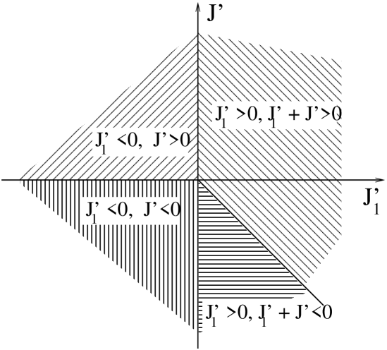
Figure 4. Phase diagram of ground states

5. Phase transition

In this section we are going to describe the existence of a phase transition for the ferromagnetic Potts model with competing interactions. We will find a critical curve under one there exists a phase transition. We also construct the Gibbs measures corresponding to the ground states $\sigma^{(i)}$ ($i=1,2,3$) in the scheme of section 3. Recall that here by a phase transition we mean the existence of at least two limiting Gibbs measures (for more definitions see [Ge],[Pr],[S]).

It should be noted that any transformation $\tau_{g}$, $g\in\Gamma^{2}_{+}$ (see (2.3)) induces a shift $\tilde{\tau}_{g}:\Omega\to\Omega$ given by the formula

$$(\tilde{\tau}_{g}\sigma)(x)=\sigma(\tau_{g}x),\ \ x\in\Gamma^{2}_{+},\ \sigma\in\Omega.$$

A Gibbs measure $\mu$ on $\Omega$ is called translation - invariant if for every $g\in\Gamma^{2}_{+}$ the equality holds $\mu(\tilde{\tau}^{-1}_{g}(A))=\mu(A)$ for all $A\in{\mathcal{F}}$, $g\in\Gamma^{2}_{+}$.

According to section 3 to show the existence of the phase transition it is enough to find two different solutions of the equation (3.61), but the analysis of solutions (3.61) is rather tricky. Therefore, it is natural to begin with translation - invariant ones, i.e. $h_{x}=h$ is constant for all $x\in V$. Such kind of solutions will describe translation-invariant Gibbs measures. In this case the equation (3.61) is reduced to the following one

(5.3) $$\left\{\begin{array}[]{ll}u=\frac{\theta_{1}^{2}\theta u^{2}+2\theta_{1}uv+\theta v^{2}+2\theta_{1}u+2v+\theta}{\theta u^{2}+2uv+\theta v^{2}+2\theta_{1}u+2\theta_{1}v+\theta_{1}^{2}\theta}\\ v=\frac{\theta u^{2}+2\theta_{1}uv+\theta_{1}^{2}\theta v^{2}+2\theta_{1}v+2u+\theta}{\theta u^{2}+2uv+\theta v^{2}+2\theta_{1}u+2\theta_{1}v+\theta_{1}^{2}\theta},\end{array}\right.$$

where $u=e^{h_{1}}$,$v=e^{h_{2}}$ for a vector $h=(h_{1},h_{2})$.

Thus for $\theta_{p}=1$ using properties of Markov random fields we get the same system of equations (3.56).

Remark 3. From (5.3) one can observe that the equation is invariant with respect to the lines $u=v$, $u=1$ and $v=1$. It is also invariant with respect to the transformation $u\to 1/u$, $v\to 1/v$. Therefore, it is enough to consider the equation on the line $v=1$, since other cases can be reduced to such a case.

So, rewrite (5.3) as follows

(5.4) $$u=f(u;\theta,\theta_{1}),$$

here

(5.5) $$f(u;\theta,\theta_{1})=\frac{\theta_{1}^{2}\theta u^{2}+4\theta_{1}u+2(\theta+1)}{\theta u^{2}+2(\theta_{1}+1)u+\theta_{1}^{2}\theta+2\theta_{1}+\theta}$$

From (5.5) we find that (5.4) reduces to the following

$$\theta u^{3}+(2\theta_{1}-\theta_{1}^{2}\theta+2)u^{2}+(\theta_{1}^{2}\theta+\theta-2\theta_{1})u-2(\theta+1)=0$$

which can be represented by

$$(u-1)\bigg{(}\theta u^{2}+(\theta_{1}+1)(\theta(1-\theta_{1})+2)u+2(\theta+1)\bigg{)}=0.$$

Thus, $u=1$ is a solution of (5.4), but to exist a phase transition we have to find other fixed points of (5.5). It means that we have to establish a condition when the following equation

(5.6) $$\theta u^{2}+(\theta_{1}+1)(\theta(1-\theta_{1})+2)u+2(\theta+1)=0$$

has two positive solutions. Of course, the last one (5.6) has the required solutions if

(5.7) $$(\theta_{1}+1)(\theta(1-\theta_{1})+2)<0,$$

(5.8) the discriminant of (5.6) is positive.

The condition (5.7) implies that

(5.9) $$\theta_{1}>1\ \ \textrm{and}\ \ \theta>\frac{2}{\theta_{1}-1}.$$

Rewrite the condition (5.8) as follows

(5.10) $$\bigg{(}(\theta_{1}^{2}-1)^{2}-8\bigg{)}\theta^{2}-4\bigg{(}(\theta_{1}+1)^{2}(\theta_{1}-1)+2\bigg{)}\theta+4(\theta_{1}+1)^{2}>0,$$

which can be represented by

(5.11) $$(\theta-\xi_{1})(\theta-\xi_{2})>0,$$

where

(5.12) $$\xi_{1,2}=\frac{2\bigg{(}(\theta_{1}+1)^{2}(\theta_{1}-1)+2\bigg{)}\mp 4\sqrt{(\theta_{1}+1)^{3}+1}}{(\theta_{1}^{2}-1)^{2}-8}.$$

From (5.10) we obtain that

(5.13) $$\xi_{1}\cdot\xi_{2}=\frac{4(\theta_{1}+1)^{2}}{(\theta_{1}^{2}-1)^{2}-8}.$$

Now we are going to compare the condition (5.9) with solution of (5.11). To do it, let us consider two cases.

Case (a). Let $(\theta_{1}^{2}-1)^{2}-8>0$. This is equivalent to $\theta_{1}>\sqrt{1+2\sqrt{2}}$. Hence, according to (5.13) we infer that both $\xi_{1}$ and $\xi_{2}$ are positive. So, the solution of (5.11) is

(5.14) $$\theta\in(0,\xi_{1})\cup(\xi_{2},\infty).$$

From (5.12) we can check that

$$\xi_{1}<\frac{2}{\theta_{1}-1}<\xi_{2}.$$

Therefore, from (5.9),(5.14) we conclude that $\theta$ should satisfy the following condition

(5.15) $$\theta>\xi_{2}\ \ \ \textrm{while}\ \ \theta_{1}>\sqrt{1+2\sqrt{2}}.$$

Case (b). Let $(\theta_{1}^{2}-1)^{2}-8<0$, then this with (5.9) yields that $1<\theta_{1}<\sqrt{1+2\sqrt{2}}$. Using (5.11) and (5.13) one can find that

(5.18) $$\left\{\begin{array}[]{ll}\theta>\xi_{1},\ \ \textrm{if}\ \ \theta^{*}<\theta_{1}<\sqrt{1+2\sqrt{2}}\\[8.53581pt] \theta>\frac{2}{\theta_{1}-1},\ \ \textrm{if}\ \ 1<\theta_{1}<\theta^{*},\end{array}\right.$$

where $\theta^{*}$ is a unique solution of the equation $(x-1)(\sqrt{(x+1)^{3}+1}-1)-4=0$.

Consequently, if one of the conditions (5.15) or (5.18) is satisfied then $f(u,;\theta,\theta_{1})$ has three fixed points $u=1$, $u^{*}_{1}$ and $u_{2}^{*}$.

Now we are interested when both $u^{*}_{1}$ and $u_{2}^{*}$ solutions are attractive. This occurs when

$$\frac{d}{du}f(u,;\theta,\theta_{1})|_{u=1}>1,$$

since the function $f(u,;\theta,\theta_{1})$ is increasing and bounded. Hence, a simple calculation shows that the last condition holds if

(5.22) $$\theta_{1}>2\ \ \textrm{and}\ \ \theta>\frac{2}{\theta_{1}-2}.$$

If $\theta_{1}>2$ then the condition (5.18) is not satisfied since $\theta^{*}<2$. Consequently, combining the conditions (5.15) and (5.22) we establish that if

(5.23) $$\theta_{1}>2\ \ \textrm{and}\ \ \theta>\max\bigg{\{}\frac{2}{\theta_{1}-2},\xi_{2}\bigg{\}},$$

then $f(u,;\theta,\theta_{1})$ has three fixed points, and two of them $u^{*}_{1}$ and $u_{2}^{*}$ are attractive. Without loss of generality we may assume that $u^{*}_{1}>u_{2}^{*}$. Then from (5.6) one sees that

$$u^{*}_{1}u_{2}^{*}=\frac{2(\theta+1)}{\theta}.$$

which implies that

(5.24) $$u^{*}_{1}\to\infty,\ \ u_{2}^{*}\to 0\ \ \textrm{as}\ \ \beta\to\infty$$

Let us denote

$$h^{*}_{1,1}=\bigg{(}\frac{2}{3}\log u^{*}_{1},0\bigg{)},\ \ h^{*}_{2,1}=\bigg{(}\frac{2}{3}\log u^{*}_{2},0\bigg{)},$$

which are translation-invariant solutions of (3.61).

According to Remark 2 the vectors

(5.25) $$\left\{\begin{array}[]{ll}h^{*}_{1,2}=(0,\frac{2}{3}\log u^{*}_{1}),\ \ h^{*}_{2,2}=(0,\frac{2}{3}\log u^{*}_{2})\\[5.69054pt] h^{*}_{1,3}=(-\frac{2}{3}\log u^{*}_{1},-\frac{2}{3}\log u^{*}_{1}),\ \ h^{*}_{2,3}=(-\frac{2}{3}\log u^{*}_{2},-\frac{2}{3}\log u^{*}_{2})\\ \end{array}\right.$$

are also translation-invariant solutions of (3.61). The Gibbs measures corresponding these solutions are denoted by $\mu_{1,i},\mu_{2,i}$, $(i=1,2,3$), respectively.

From (5.23) we infer that $(J,J_{1})$ belongs to $B_{1}$. Furthermore, we assume that (5.23) is satisfied. This means in this case there are three ground states for the model. Therefore, when $\beta\to\infty$ certain measures $\mu_{1,i},\mu_{2,i}$ should tend to the ground states $\{\sigma^{(1)},\sigma^{(2)},\sigma^{(3)}\}$. Let us choose those ones. Take $\mu_{1,1}$, then from (3.58), (2.9) and (5.24) we have

(5.26) $$\mu_{1,1}(\sigma(x)=\eta_{1}) = \displaystyle\frac{e^{h^{*}_{1,1}\eta_{1}}}{e^{h^{*}_{1,1}\eta_{1}}+e^{h^{*}_{1,1}\eta_{2}}+e^{h^{*}_{1,1}\eta_{3}}}$$

$$= \displaystyle\frac{u^{*}_{1}}{u^{*}_{1}+2}\to 1\ \ \textrm{as}\ \beta\to\infty,$$

where $x\in V$.

Similarly, using the same argument we may find

(5.27) $$\mu_{1,2}(\sigma(x)=\eta_{2})\to 1,\ \ \mu_{1,3}(\sigma(x)=\eta_{3})\to 1\ \ \textrm{as}\ \beta\to\infty.$$

Denote these measures by $\mu_{k}=\mu_{1,k}$, $k=1,2,3$. The relations (5.26),(5.27) prompt that the following should be true

$$\mu_{i}\to\delta_{\sigma^{(i)}}\ \ \ \textrm{as}\ \ \beta\to\infty,$$

here $\delta_{\sigma}$ is a delta-measure concentrated on $\sigma$. Indeed, let us without loss of generality consider the measure $\mu_{1}$. We know that $\sigma^{(1)}$ is a ground state, therefore according to Proposition 4.1 one gets that $H(\sigma_{n}|_{V_{n}})\geq H(\sigma^{(1)}|_{V_{n}})$ for all $\sigma\in\Omega$ and $n>0$. Hence, it follows from (3.58) that

$$\mu_{1}(\sigma^{(1)}|_{V_{n}}) = \frac{\exp\{-\beta H(\sigma^{(1)}|_{V_{n}})+h^{*}_{1,1}\eta_{1}|W_{n}|\}}{\sum\limits_{\tilde{\sigma}_{n}\in\Omega_{V_{n}}}\exp\{-\beta H(\tilde{\sigma}_{n})+h^{*}_{1,1}\sum\limits_{x\in W_{n}}\tilde{\sigma}(x)\}}$$

$$= \frac{1}{1+\sum\limits_{\tilde{\sigma}_{n}\in\Omega_{V_{n}},\tilde{\sigma}_{n}\neq\sigma^{(1)}|_{V_{n}}}\frac{\exp\{-\beta H(\tilde{\sigma}_{n})+h^{*}_{1,1}\sum\limits_{x\in W_{n}}\tilde{\sigma}(x)\}}{\exp\{-\beta H(\sigma^{(1)}|_{V_{n}})+h^{*}_{1,1}\eta_{1}|W_{n}|\}}}$$

$$\geq \frac{1}{1+1/u^{*}_{1}}\to 1\ \ \textrm{as}\ \beta\to\infty.$$

The last inequality yields that the required relation.

Consequently, the measures $\mu_{k}$ ($k=1,2,3$) describe pure phases of the model.

Let us find the critical temperature. To do it, rewrite (5.23) as follows:

(5.28) $$\frac{T}{J_{1}}<\frac{1}{\log 2},\ \ \ \frac{J}{J_{1}}>\max\bigg{\{}\varphi\bigg{(}\frac{T}{J_{1}}\bigg{)},\zeta\bigg{(}\frac{T}{J_{1}}\bigg{)}\bigg{\}},$$

where

$$\varphi(x) = x\log\bigg{(}\frac{2}{\exp(1/x)-2}\bigg{)}$$

$$\zeta(x) = x\log\left(\frac{2\bigg{(}(\exp(1/x)+1)^{2}(\exp(1/x)-1)+2\bigg{)}+4\sqrt{(\exp(1/x)+1)^{3}+1}}{(\exp(2/x)-1)^{2}-8}\right).$$

From these relations one concludes that the critical line (see Fig.5) is given by

(5.29) $$\frac{T_{c}}{J_{1}}=\min\bigg{\{}\varphi^{-1}\bigg{(}\frac{J}{J_{1}}\bigg{)},\zeta^{-1}\bigg{(}\frac{J}{J_{1}}\bigg{)}\bigg{\}}$$

Consequently, we can formulate the following

Theorem 5.1.

If the condition (5.28) is satisfied for the three state Potts model (3.57) on the second ordered Bethe lattice, then there exists a phase transition and three pure translation-invariant phases.

Figure 5. The curve $\frac{T_{c}}{J_{1}}=\min\bigg{\{}\varphi^{-1}\bigg{(}\frac{J}{J_{1}}\bigg{)},\zeta^{-1}\bigg{(}\frac{J}{J_{1}}\bigg{)}\bigg{\}}$ in the plane $(\frac{J}{J_{1}},\frac{T}{J_{1}})$

.

Remark 4. If we put $J=0$ to the condition (5.23) then the obtained result agrees with the results of [PLM1, PLM2], [G].

Observation. From (5.19)-(5.21) we can derive that the eigenvalues of the Jacobian at the fixed points $(u_{1}^{*},1)$, $(1,u_{1}^{*})$, $(u_{2}^{*},1)$, $(1,u_{2}^{*})$, $((u_{1}^{*})^{-1},(u_{1}^{*})^{-1})$, $((u_{2}^{*})^{-1},(u_{2}^{*})^{-1})$ are real. Therefore, in this case (i.e. $J_{p}=0$), there are not the modulated phases and Lifshitz points. On the other hand, the absolute value of the eigenvalues of the Jacobian at the fixed points $(u_{1}^{*},1)$, $(1,u_{1}^{*})$ and $((u_{1}^{*})^{-1},(u_{1}^{*})^{-1})$ are smaller than 1. The absolute value of the eigenvalues at the fixed points $(u_{2}^{*},1)$, $(1,u_{2}^{*})$ and $((u_{2}^{*})^{-1},(u_{2}^{*})^{-1})$ are bigger than 1. These show that the points $(u_{1}^{*},1)$, $(1,u_{1}^{*})$ and $((u_{1}^{*})^{-1},(u_{1}^{*})^{-1})$ are the stable fixed points of the transformation given by (5.3). The Gibbs measures associated with these points are pure phases.

Remark 5. Recall that the a Gibbs measure $\mu_{0}$ corresponding to the solution $h=(0,0)$ is called unordered phase. The purity of the unordered phase was investigated in [GR],[MR3] when $J=0$. Such a property relates to the reconstruction thresholds and percolation on lattices (see [Mar],[JM]). For $J\neq 0$ the purity of $\mu_{0}$ is an open problem.

6. A formula of the free energy

This section is devoted to the free energy and exact calculation of certain physical quantities. Since the Bethe lattice is non-amenable, so we have to prove the existence of the free energy.

Consider the partition function $Z^{(n)}(\beta,h)$ (see (3.59)) of the Gibbs measure $\mu^{h}_{\beta}$ (which corresponds to solution $h=\{h_{x},x\in V\}$ of the equation (3.61))

$$Z^{(n)}(\beta,h)=\sum_{\tilde{\sigma}_{n}\in\Omega_{V_{n}}}\exp\{-\beta H(\tilde{\sigma}_{n})+\sum_{x\in W_{n}}h_{x}\tilde{\sigma}_{n}(x)\}.$$

The free energy is defined by

(6.1) $$F_{\beta}(h)=-\lim_{n\to\infty}{1\over 3\beta\cdot 2^{n}}\ln Z^{(n)}(\beta,h).$$

The goal of this section is to prove following:

Theorem 6.1.

The free energy of the model (3.57) exists for all $h$, and is given by the formula

(6.2) $$F_{\beta}(h)=-\lim_{n\to\infty}{1\over 3\beta\cdot 2^{n}}\sum_{k=0}^{n}\sum_{x\in W_{n-k}}\log a(x,h_{y},h_{z};\theta,\theta_{1},\beta),$$

where $y=y(x),z=z(x)$ are direct successors of $x$;

(6.3) $$a(x,h_{y},h_{z};\theta,\theta_{1},\beta)=e^{-(J/2+J_{1})\beta}g(h^{\prime}_{y},h^{\prime}_{z})\bigg{[}F(h^{\prime}_{y},h^{\prime}_{z})F((h^{\prime}_{y})^{t},(h^{\prime}_{z})^{t})\bigg{]}^{1/3},$$

here the function $F(h,r)$ is defined as in (3.62), and

$$g(h,r)=\theta e^{h_{1}+r_{1}}+e^{h_{1}+r_{2}}+e^{h_{2}+r_{1}}+\theta e^{h_{2}+r_{2}}+\theta_{1}(e^{h_{1}}+e^{r_{1}}+e^{h_{2}}+e^{r_{2}})+\theta_{1}^{2}\theta,$$

where $h=(h_{1},h_{2}),r=(r_{1},r_{2})$.

Proof.

We shall use the recursive equation (B.6), i.e.

$$Z^{(n)}=A_{n-1}Z^{(n-1)},$$

where $A_{n}=\prod\limits_{x\in W_{n}}a(x,h_{y},h_{z};\theta,\theta_{1},\beta)$ $x\in V$, $y,z\in S(x)$, which is defined below. Using (B.3) we have (6.3).

Thus, the recursive equation (B.6) has the following form

(6.4) $$Z^{(n)}(\beta;h)=\exp\bigg{(}\sum_{x\in W_{n-1}}\log a(x,h_{y},h_{z};\theta,\theta_{1},\beta)\bigg{)}Z^{(n-1)}(\beta,h).$$

Now we prove existence of the RHS limit of (6.2). From the form of the function $F$ one gets that it is bounded, i.e. $|F(h,r)|\leq M$ for all $h,r\in{\mathbb{R}}^{2}$. Hence, we conclude that the solutions of the equation (3.61) are bounded, i.e. $|h_{x,i}|\leq C$ for all $x\in V$, $i=1,2$. Here $C$ is some constant and $h_{x}=(h_{x,1}h_{x,2})$. Consequently the function $a(x,h_{y},h_{z};\theta,\theta_{1},\beta)$ is bounded, and so $|\log a(x,h_{y},h_{z};\theta,\theta_{1},\beta)|\leq C_{\beta}$ for all $h_{y},h_{z}$. Hence we get

$${1\over 3\cdot 2^{n}}\sum_{k=l+1}^{n}\sum_{x\in W_{n-k}}\log a(x,h_{y},h_{z};\theta,\theta_{1},\beta)$$

(6.5) $$\leq{C_{\beta}\over 2^{n}}\sum_{k=l+1}^{n}2^{n-k-1}\leq C_{\beta}\cdot 2^{-l}.$$

Therefore, from (6) we get the existence of the limit at RHS of (6.2). ∎

Let us compute the free energy corresponding the measures $\mu_{i}$, ($i=1,2,3$). Assuming first that $h_{x}=h$ for all $x\in V$. Then from (6.2) and (6.3) one gets

$$F_{\beta}(h)=\frac{1}{\beta}\log a(h,\theta,\theta_{1},\beta),$$

here

(6.6) $$a(h,\theta,\theta_{1},\beta)=e^{-(J/2+J_{1})\beta}g(h^{\prime},h^{\prime})\bigg{[}F(h^{\prime},h^{\prime})F((h^{\prime})^{t},(h^{\prime})^{t})\bigg{]}^{1/3}.$$

Let us consider $h=h^{*}_{1,k}$, ($k=1,2,3$). Denote $F_{\beta}=F_{\beta}(h^{*}_{1,k})$. Then we have

(6.7) $$\beta F_{\beta}=\log\bigg{[}e^{-(J/2+J_{1})\beta}(u^{*}_{1})^{1/3}(\theta(u^{*}_{1})^{2}+2(\theta_{1}+1)u^{*}_{1}+\theta_{1}^{2}\theta+2\theta_{1}+\theta)\bigg{]}.$$

Taking into account (5.6) the equality (6.8) can be rewritten as follows:

(6.8) $$\beta F_{\beta}=-(J/2+J_{1})\beta+\frac{1}{3}\log u^{*}_{1}+\log(\theta_{1}-1)+\log\bigg{[}\theta(\theta_{1}+1)(u^{*}_{1}+1)+2\bigg{]}.$$

Now let us compute the internal energy $U$ of the model. It is known that the following formula holds

(6.9) $$U=\frac{\partial(\beta F_{\beta})}{\partial\beta}.$$

Before compute it we have to calculate $du^{*}_{1}/d\beta$. Taking derivation from both sides of (5.6) one finds

(6.10) $$\frac{du^{*}_{1}}{d\beta}=\frac{3\bigg{(}(J_{1}\theta_{1}(\theta\theta_{1}-1)+J(\theta_{1}+1))u^{*}_{1}+J\bigg{)}}{2\theta u^{*}_{1}+(\theta_{1}+1)(\theta(1-\theta_{1})+2)}.$$

From (6.8) and (6.9) we obtain

$$U = -(J/2+J_{1})+\frac{3}{2}\bigg{[}\frac{J_{1}}{\theta_{1}-1}+\frac{\theta((J+J_{1})\theta_{1}+J)(u^{*}_{1}+1)}{\theta(\theta_{1}+1)(u^{*}_{1}+1)+2}\bigg{]}$$

$$+\bigg{[}\frac{\theta(\theta_{1}+1)(4u^{*}_{1}+1)+2}{3u^{*}_{1}(\theta(\theta_{1}+1)(u^{*}_{1}+1)+2)}\bigg{]}\frac{du^{*}_{1}}{d\beta}$$

Again using (5.6) and (6.10) one gets

$$U = -(J/2+J_{1})+\frac{3}{2}\bigg{[}\frac{\theta\theta_{1}(J_{1}(\theta^{2}_{1}+1)+J(\theta_{1}-1))(u^{*}_{1}+1)+2J_{1}}{\theta(\theta^{2}_{1}-1)(u^{*}_{1}+1)+2(\theta_{1}-1)}\bigg{]}$$

$$+\bigg{[}\frac{\theta(\theta_{1}+1)(4u^{*}_{1}+1)+2}{(\theta(\theta_{1}+1)(\theta\theta_{1}-2)-2)u^{*}_{1}-2(\theta+1)(\theta_{1}+1)}\bigg{]}$$

$$\times\bigg{[}\frac{((J_{1}\theta_{1}(\theta\theta_{1}-1)+J(\theta_{1}+1))u^{*}_{1}+J)}{2\theta u^{*}_{1}+(\theta_{1}+1)(\theta(1-\theta_{1})+2)}\bigg{]}$$

Using this expression we can also calculate entropy of the model.

Since spins take values in ${\mathbb{R}}^{2}$, therefore the magnetization of the model would be ${\mathbb{R}}^{2}$-valued quantity. Using the result of sections 4 and 5 we can easily compute the magnetization. Let us calculate it with respect to the measure $\mu_{1}$. Note that the model is translation-invariant, therefore, we have $M_{1}=<\sigma_{(0)}>_{\mu_{1}}$, so using (2.9), (2.8) and (3.58) one finds

$$M_{1} = \eta_{1}\mu_{1}(\sigma_{(0)}=\eta_{1})+\eta_{2}\mu_{1}(\sigma_{(0)}=\eta_{2})+\eta_{3}\mu_{1}(\sigma_{(0)}=\eta_{3})$$

$$= \frac{1}{(u_{1}^{*})^{2/3}+2(u_{1}^{*})^{-1/3}}\bigg{(}\eta_{1}(u_{1}^{*})^{2/3}+\eta_{2}(u_{1}^{*})^{-1/3}+\eta_{3}(u_{1}^{*})^{-1/3}\bigg{)}$$

$$= \frac{1}{u_{1}^{*}+2}\bigg{(}\eta_{1}u_{1}^{*}+\eta_{2}+\eta_{3}\bigg{)}$$

$$= \frac{u_{1}^{*}-1}{u_{1}^{*}+2}\eta_{1}.$$

Similarly, one gets

$$M_{2}=<\sigma_{(0)}>_{\mu_{2}} = \frac{u_{1}^{*}-1}{u_{1}^{*}+2}\eta_{2}.$$

$$M_{3}=<\sigma_{(0)}>_{\mu_{3}} = \frac{u_{1}^{*}-1}{2u_{1}^{*}+1}\eta_{3}.$$

7. Discussion of results

It is known [Ba] that to exact calculations in statistical mechanics are paid attention by many of researchers, because those are important not only for their own interest but also for some deeper understanding of the critical properties of spin systems which are not obtained form approximations. So, those are very useful for testing the credibility and efficiency of any new method or approximation before it is applied to more complicated spin systems. In the present paper we have derived recurrent equations for the partition functions of the three state Potts model with competing interactions on a Bethe lattice of order two, and certain particular cases of those equations were studied. In the presence of the one-level competing interactions we exactly solved the ferromagnetic Potts model. The critical curve (5.29) such that there exits a phase transitions under it, was calculated (see Fig. 5). It has been described the set of ground states of the model (see Fig. 4). This shows that the ground states of the model are richer than the ordinary Potts model on the Bethe lattice. Using this description and the recurrent equations, one found the Gibbs measures associated with the translation-invariant ground states. Note that such Gibbs measures determine generalized 2-step Markov chains (see [D]). Moreover, we proved the existence of the free energy, and exactly calculated it for those measures. Besides, we have computed some other physical quantities too. The results agrees with [PLM1, PLM2], [G] when we neglect the next nearest neighbor interactions.

Note that for the Ising model on the Bethe lattice with in the presence of the one-level and prolonged competing interactions the modulated phases and Lifshitz points appear in the phase diagram (see [V],[YOS],[SC]). In absence of the prolonged competing interactions in the 3-state Potts model we do not have such kind of phases, this means one-level interactions could not affect the appearance the modulated phases. One can hope that the considered Potts model with $J_{p}=0$ will describe some biological models. Note that the case, when the prolonged competing interaction is nontrivial ($J_{p}\neq 0$), will be a theme of our next investigations [GMMP], where the modulated phases and Lifshitz points will be discussed.

Appendix A Recurrent equations at $J_{p}\neq 0$

Denote

(A.10) $$\left\{\begin{array}[]{lll}A^{(n)}_{1}&=&\theta^{2}_{p}Z^{(n)}_{1}+\theta_{p}Z^{(n)}_{2}+\theta_{p}Z^{(n)}_{3}+\theta_{p}Z^{(n)}_{4}+Z^{(n)}_{5}+Z^{(n)}_{6}+\theta_{p}Z^{(n)}_{7}+Z^{(n)}_{8}+Z^{(n)}_{9},\\ B^{(n)}_{1}&=&\theta^{2}_{p}Z^{(n)}_{10}+\theta_{p}Z^{(n)}_{11}+\theta_{p}Z^{(n)}_{12}+\theta_{p}Z^{(n)}_{13}+Z^{(n)}_{14}+Z^{(n)}_{15}+\theta_{p}Z^{(n)}_{16}+Z^{(n)}_{17}+Z^{(n)}_{18},\\ C^{(n)}_{1}&=&\theta^{2}_{p}Z^{(n)}_{19}+\theta_{p}Z^{(n)}_{20}+\theta_{p}Z^{(n)}_{21}+\theta_{p}Z^{(n)}_{22}+Z^{(n)}_{23}+Z^{(n)}_{24}+\theta_{p}Z^{(n)}_{25}+Z^{(n)}_{26}+Z^{(n)}_{27},\\ A^{(n)}_{2}&=&Z^{(n)}_{1}+\theta_{p}Z^{(n)}_{2}+Z^{(n)}_{3}+\theta_{p}Z^{(n)}_{4}+\theta_{p}^{2}Z^{(n)}_{5}+\theta_{p}Z^{(n)}_{6}+Z^{(n)}_{7}+\theta_{p}Z^{(n)}_{8}+Z^{(n)}_{9},\\ B^{(n)}_{2}&=&Z^{(n)}_{10}+\theta_{p}Z^{(n)}_{11}+Z^{(n)}_{12}+\theta_{p}Z^{(n)}_{13}+\theta_{p}^{2}Z^{(n)}_{14}+\theta_{p}Z^{(n)}_{15}+Z^{(n)}_{16}+\theta_{p}Z^{(n)}_{17}+Z^{(n)}_{18},\\ C^{(n)}_{2}&=&Z^{(n)}_{19}+\theta_{p}Z^{(n)}_{20}+Z^{(n)}_{21}+\theta_{p}Z^{(n)}_{22}+\theta_{p}^{2}Z^{(n)}_{23}+\theta_{p}Z^{(n)}_{24}+Z^{(n)}_{25}+\theta_{p}Z^{(n)}_{26}+Z^{(n)}_{27},\\ A^{(n)}_{3}&=&Z^{(n)}_{1}+Z^{(n)}_{2}+\theta_{p}Z^{(n)}_{3}+Z^{(n)}_{4}+Z^{(n)}_{5}+\theta_{p}Z^{(n)}_{6}+\theta_{p}Z^{(n)}_{7}+\theta_{p}Z^{(n)}_{8}+\theta_{p}^{2}Z^{(n)}_{9},\\ B^{(n)}_{3}&=&Z^{(n)}_{10}+Z^{(n)}_{11}+\theta_{p}Z^{(n)}_{12}+Z^{(n)}_{13}+Z^{(n)}_{14}+\theta_{p}Z^{(n)}_{15}+\theta_{p}Z^{(n)}_{16}+\theta_{p}Z^{(n)}_{17}+\theta_{p}^{2}Z^{(n)}_{18},\\ C^{(n)}_{3}&=&Z^{(n)}_{19}+Z^{(n)}_{20}+\theta_{p}Z^{(n)}_{21}+Z^{(n)}_{22}+Z^{(n)}_{23}+\theta_{p}Z^{(n)}_{24}+\theta_{p}Z^{(n)}_{25}+\theta_{p}Z^{(n)}_{26}+\theta_{p}^{2}Z^{(n)}_{27},\end{array}\right.$$

then the last one in terms of (3.37) is represented by

(A.20) $$\left\{\begin{array}[]{lll}A^{(n)}_{1}&=&\theta_{p}^{2}x^{(n)}_{1}+2\theta_{p}x^{(n)}_{2}+2\theta_{p}x^{(n)}_{3}+x^{(n)}_{4}+2x^{(n)}_{5}+x^{(n)}_{6},\\ B^{(n)}_{1}&=&\theta_{p}^{2}x^{(n)}_{7}+2\theta_{p}x^{(n)}_{8}+2\theta_{p}x^{(n)}_{9}+x^{(n)}_{10}+2x^{(n)}_{11}+x^{(n)}_{12},\\ C^{(n)}_{1}&=&\theta_{p}^{2}x^{(n)}_{13}+2\theta_{p}x^{(n)}_{14}+2\theta_{p}x^{(n)}_{15}+x^{(n)}_{16}+2x^{(n)}_{17}+x^{(n)}_{18},\\ A^{(n)}_{2}&=&x^{(n)}_{1}+2\theta_{p}x^{(n)}_{2}+2x^{(n)}_{3}+\theta^{2}_{p}x^{(n)}_{4}+2x^{(n)}_{5}+x^{(n)}_{6},\\ B^{(n)}_{2}&=&x^{(n)}_{7}+2\theta_{p}x^{(n)}_{8}+2x^{(n)}_{9}+\theta^{2}_{p}x^{(n)}_{10}+2x^{(n)}_{11}+x^{(n)}_{12},\\ C^{(n)}_{2}&=&x^{(n)}_{13}+2\theta_{p}x^{(n)}_{14}+2x^{(n)}_{15}+\theta^{2}_{p}x^{(n)}_{16}+2x^{(n)}_{17}+x^{(n)}_{18},\\ A^{(n)}_{3}&=&x^{(n)}_{1}+2x^{(n)}_{2}+2\theta_{p}x^{(n)}_{3}+x^{(n)}_{4}+2\theta_{p}x^{(n)}_{5}+\theta_{p}^{2}x^{(n)}_{6},\\ B^{(n)}_{3}&=&x^{(n)}_{7}+2x^{(n)}_{8}+2\theta_{p}x^{(n)}_{9}+x^{(n)}_{10}+2\theta_{p}x^{(n)}_{11}+\theta_{p}^{2}x^{(n)}_{12},\\ C^{(n)}_{3}&=&x^{(n)}_{13}+2x^{(n)}_{14}+2\theta_{p}x^{(n)}_{15}+x^{(n)}_{16}+2\theta_{p}x^{(n)}_{17}+\theta_{p}^{2}x^{(n)}_{18}.\end{array}\right.$$

From (3.20),(A.10) and (A.20) we obtain

$$A^{(n)}_{1} = \tilde{Z}^{(n)}_{1}+(\theta_{p}^{2}-1)x^{(n)}_{1}+2(\theta_{p}-1)x^{(n)}_{2}+2(\theta_{p}-1)x^{(n)}_{3},$$

$$B^{(n)}_{1} = \tilde{Z}^{(n)}_{2}+(\theta_{p}^{2}-1)x^{(n)}_{7}+2(\theta_{p}-1)x^{(n)}_{8}+2(\theta_{p}-1)x^{(n)}_{9},$$

$$C^{(n)}_{1} = \tilde{Z}^{(n)}_{3}+(\theta_{p}^{2}-1)x^{(n)}_{13}+2(\theta_{p}-1)x^{(n)}_{14}+2(\theta_{p}-1)x^{(n)}_{15},$$

$$A^{(n)}_{2} = \tilde{Z}^{(n)}_{1}+2(\theta_{p}-1)x^{(n)}_{2}+(\theta_{p}^{2}-1)x^{(n)}_{4}+2(\theta_{p}-1)x^{(n)}_{5},$$

$$B^{(n)}_{2} = \tilde{Z}^{(n)}_{2}+2(\theta_{p}-1)x^{(n)}_{8}+(\theta_{p}^{2}-1)x^{(n)}_{10}+2(\theta_{p}-1)x^{(n)}_{11},$$

$$C^{(n)}_{2} = \tilde{Z}^{(n)}_{3}+2(\theta_{p}-1)x^{(n)}_{14}+(\theta_{p}^{2}-1)x^{(n)}_{16}+2(\theta_{p}-1)x^{(n)}_{17},$$

$$A^{(n)}_{3} = \tilde{Z}^{(n)}_{1}+2(\theta_{p}-1)x^{(n)}_{3}+2(\theta_{p}-1)x^{(n)}_{5}+(\theta_{p}^{2}-1)x^{(n)}_{6},$$

$$B^{(n)}_{3} = \tilde{Z}^{(n)}_{2}+2(\theta_{p}-1)x^{(n)}_{9}+2(\theta_{p}-1)x^{(n)}_{11}+(\theta_{p}^{2}-1)x^{(n)}_{12},$$

$$C^{(n)}_{3} = \tilde{Z}^{(n)}_{3}+2(\theta_{p}-1)x^{(n)}_{15}+2(\theta_{p}-1)x^{(n)}_{17}+(\theta_{p}^{2}-1)x^{(n)}_{18}.$$

Now let us assume that $J_{p}\neq 0$ and $\bar{\sigma}\equiv\eta_{1}$. Then

$$B_{1}^{(n)}=C_{1}^{(n)},\quad A_{2}^{(n)}=A_{3}^{(n)},$$

$$B_{2}^{(n)}=C_{3}^{(n)},\quad B_{3}^{(n)}=C_{2}^{(n)},$$

and

$$\tilde{Z}_{2}^{(n)}=\tilde{Z}_{3}^{(n)}.$$

Hence the recurrence system (3.47) has the following form

(A.29) $$\left\{\begin{array}[]{ll}x^{(n+1)}_{1}=\theta\theta_{1}^{2}(A^{(n)}_{1})^{2},&x^{(n+1)}_{2}=x^{(n+1)}_{3}=\theta_{1}A^{(n)}_{1}B^{(n)_{1}},\\ x^{(n+1)}_{4}=x^{(n+1)}_{6}=\theta(B^{(n)}_{1})^{2},&x^{(n+1)}_{5}=(B^{(n)}_{1})^{2},\\ x^{(n+1)}_{7}=\theta(A^{(n)}_{2})^{2},&x^{(n+1)}_{8}=\theta_{1}A^{(n)}_{2}B^{(n)}_{2},\\ x^{(n+1)}_{9}=A^{(n)}_{2}C^{(n)}_{2},&x^{(n+1)}_{10}=\theta\theta_{1}^{2}(B^{(n)}_{2})^{2},\\ x^{(n+1)}_{11}=\theta_{1}B^{(n)}_{2}C^{(n)}_{2},&x^{(n+1)}_{12}=\theta(C_{2}^{(n)})^{2},\\ x^{(n+1)}_{13}=x^{(n+1)}_{7},&x^{(n+1)}_{14}=x^{(n+1)}_{9},\\ x^{(n+1)}_{15}=x^{(n+1)}_{8},&x^{(n+1)}_{16}=x^{(n+1)}_{12},\\ x^{(n+1)}_{17}=x^{(n+1)}_{11},&x^{(n+1)}_{18}=x^{(n+1)}_{10}.\end{array}\right.$$

Through introducing new variables

$$\left\{\begin{array}[]{ll}y^{(n)}_{1}=x^{(n)}_{1},&y^{(n)}_{2}=x^{(n)}_{2}=x^{(n)}_{3},\\ y^{(n)}_{3}=x^{(n)}_{5}=\frac{x^{(n)}_{4}}{\theta}=\frac{x^{(n)}_{6}}{\theta},&\\ y^{(n)}_{4}=x^{(n)}_{7}=x^{(n)}_{13},&y^{(n)}_{5}=x^{(n)}_{8}=x^{(n)}_{15},\\ y^{(n)}_{6}=x^{(n)}_{9}=x^{(n)}_{14},&y^{(n)}_{7}=x^{(n)}_{10}=x^{(n)}_{18},\\ y^{(n)}_{8}=x^{(n)}_{11}=x^{(n)}_{17},&y^{(n)}_{9}=x^{(n)}_{12}=x^{(n)}_{16},\end{array}\right.$$

the recurrence system (A.29) takes the following form

$$\left\{\begin{array}[]{ll}y^{(n+1)}_{1}=\theta\theta_{1}^{2}(\tilde{A}^{(n)}_{1})^{2},&y^{(n+1)}_{2}=\theta_{1}\tilde{A}^{(n)}_{1}\tilde{B}^{(n)}_{1},\\ y^{(n+1)}_{3}=(\tilde{B}^{(n)}_{1})^{2},&y^{(n+1)}_{4}=\theta(\tilde{A}^{(n)}_{2})^{2},\\ y^{(n+1)}_{5}=\theta_{1}\tilde{A}^{(n)}_{2}\tilde{B}^{(n)}_{2},&y^{(n+1)}_{6}=\tilde{A}^{(n)}_{2}\tilde{C}^{(n)}_{2},\\ y^{(n+1)}_{7}=\theta\theta_{1}^{2}(\tilde{B}^{(n)}_{2})^{2},&y^{(n+1)}_{8}=\theta_{1}\tilde{B}^{(n)}_{2}\tilde{C}^{(n)}_{2},\\ y^{(n+1)}_{9}=\theta(\tilde{C}_{2}^{(n)})^{2},&\end{array}\right.$$

where

$$\tilde{A}^{(n)}_{1} = \theta_{p}^{2}y^{(n)}_{1}+4\theta_{p}y^{(n)}_{2}+2(\theta+1)y^{(n)}_{3},$$

$$\tilde{B}^{(n)}_{1} = \theta_{p}^{2}y^{(n)}_{4}+2\theta_{p}y^{(n)}_{5}+2\theta_{p}y^{(n)}_{6}+y^{(n)}_{7}+2y^{(n)}_{8}+y^{(n)}_{9},$$

$$\tilde{A}^{(n)}_{2} = y^{(n)}_{1}+(2\theta_{p}+1)y^{(n)}_{8}+(\theta_{p}^{2}\theta+2\theta_{p}+\theta)y^{(n)}_{3},$$

$$\tilde{B}^{(n)}_{2} = y^{(n)}_{4}+2\theta_{p}y^{(n)}_{5}+2y^{(n)}_{6}+\theta_{p}^{2}y^{(n)}_{7}+2\theta_{p}y^{(n)}_{8}+y^{(n)}_{9},$$

$$\tilde{C}^{(n)}_{2} = y^{(n)}_{4}+2\theta_{p}y^{(n)}_{6}+2y^{(n)}_{5}+\theta_{p}^{2}y^{(n)}_{9}+2\theta_{p}y^{(n)}_{8}+y^{(n)}_{7}.$$

Noting that

$$\begin{array}[]{ll}\theta(y^{(n)}_{2})^{2}=y^{(n)}_{1}y^{(n)}_{3},&\theta^{2}(y^{(n)}_{5})^{2}=y^{(n)}_{4}y^{(n)}_{7},\\ \theta^{2}(y^{(n)}_{6})^{2}=y^{(n)}_{4}y^{(n)}_{9},&\theta^{2}(y^{(n)}_{8})^{2}=y^{(n)}_{7}y^{(n)}_{9},\end{array}$$

we see that only five independent variables remain.

It should be noted that if $\theta_{1}=1$, i.e. $J_{1}=0$, then for the boundary condition $\bar{\sigma}\equiv\eta_{1}$ we have

$$A_{1}^{(n)}=A_{2}^{(n)}=A_{3}^{(n)}=\theta_{p}^{4}B_{1}^{(n)},$$

$$B_{1}^{(n)}=B_{2}^{(n)}=B_{3}^{(n)}=C_{1}^{(n)}=C_{2}^{(n)}=C_{3}^{(n)},$$

$$\tilde{Z}_{2}^{(n)}=\tilde{Z}_{3}^{(n)},$$

so that

$$\frac{\tilde{Z}_{1}^{(n+1)}}{\tilde{Z}_{3}^{(n+1)}}=\frac{\theta(\theta_{p}^{4}B_{1}^{(n)})^{2}+4(\theta_{p}^{4}B_{1}^{(n)})B_{1}^{(n)}+2(\theta+1)(B_{1}^{(n)})^{2}}{\theta(\theta_{p}^{4}B_{1}^{(n)})^{2}+4(\theta_{p}^{4}B_{1}^{(n)})B_{1}^{(n)}+2(\theta+1)(B_{1}^{(n)})^{2}}=1.$$

Consequently, when $\theta_{1}=1$ for any boundary condition exists single limit Gibbs measure, namely, the unordered phase. So that the phase transition does not occur.

Appendix B Proof of the consistency condition

In this section we show that the condition (3.60) and (3.61) are equivalent. Assume that (3.60) holds. Then inserting (3.58) into (3.60) we find

$$\frac{Z^{(n-1)}}{Z^{(n)}}\prod_{x\in W_{n-1}}\sum_{\sigma_{x}^{(n)}}\exp\{\beta J_{1}\sigma(x)(\sigma(y)+\sigma(z))+\beta J\sigma(y)\sigma(z)$$

(B.1) $$+h_{y}\sigma(y)+h_{z}\sigma(z)\}=\prod_{x\in W_{n-1}}\exp\{h_{x}\sigma(x)\},$$

here given $x\in W_{n-1}$ we denoted $S(x)=\{y,z\},\ \ \sigma_{x}^{(n)}=\{\sigma(y),\sigma(z)\}$ and used $\sigma^{(n)}=\bigcup\limits_{x\in W_{n-1}}\sigma_{x}^{(n)}.$

Now fix $x\in W_{n-1}$ and rewrite (B) for the cases $\sigma(x)=\eta_{i}$ ($i=1,2$) and $\sigma(x)=\eta_{3}$, and then taking their rations we find

$${\sum_{\sigma_{x}^{(n)}=\{\sigma(y),\sigma(z)\}}\exp\{\beta J_{1}\eta_{i}(\sigma(y)+\sigma(z))+\beta J\sigma(y)\sigma(z)+h_{y}\sigma(y)+h_{z}\sigma(z)\}\over\sum_{\sigma_{x}^{(n)}=\{\sigma(y),\sigma(z)\}}\exp\{-\beta J_{1}\eta_{3}(\sigma(y)+\sigma(z))+\beta J\sigma(y)\sigma(z)+h_{y}\sigma(y)+h_{z}\sigma(z)\}}$$

(B.2) $$=\exp\{h^{\prime}_{x,i}\}.$$

Now by using (2.9) from (B) we get

(B.3) $$e^{h_{x,1}^{\prime}}=F(h_{y}^{\prime},h_{z}^{\prime}),\ \ \ e^{h_{x,2}^{\prime}}=F((h_{y}^{\prime})^{t},(h_{z}^{\prime})^{t}).$$

From the equality (B.3) we conclude that the function ${\mathbf{h}}=\{h_{x}=(h_{x,1},h_{x,2}):x\in V\}$ should satisfy (3.61).

Note that the converse is also true, i.e. if (3.61) holds that measures defined by (3.58) satisfy the consistency condition. Indeed, the equality (3.61) implies (B.3), and hence (B). From (B) we obtain

$$\sum_{\sigma_{x}^{(n)}=\{\sigma(y),\sigma(z)\}}\exp\{\beta J_{1}\eta_{i}(\sigma(y)+\sigma(z))+\beta J\sigma(y)\sigma(z)+h_{y}\sigma(y)+h_{z}\sigma(z)\}$$

$$=a(x)\exp\{\eta_{i}h_{x}\},$$

where $i=1,2,3$ and $a(x)$ is some function. This equality implies

$$\prod_{x\in W_{n-1}}\sum_{\sigma_{x}^{(n)}=\{\sigma(y),\sigma(z)\}}\exp\{\beta J_{1}(\sigma(y)+\sigma(z))\sigma(x)+\beta J\sigma(y)\sigma(z)+h_{y}\sigma(y)+h_{z}\sigma(z)\}$$

(B.4) $$=\prod_{x\in W_{n-1}}a(x)\exp\{\sigma(x)h_{x}\}.$$

Writing $A_{n}=\prod_{x\in W_{n}}a(x)$ from (B) one gets

(B.5) $$Z^{(n-1)}A_{n-1}\mu^{(n-1)}(\sigma_{n-1})=Z^{(n)}\sum_{\sigma^{(n)}}\mu_{n}(\sigma_{n-1}\vee\sigma^{(n)}).$$

Taking into account that each $\mu^{(n)},\ \ n\geq 1$ is a probability measure, i.e.

$$\sum_{\sigma_{n-1}}\sum_{\sigma^{(n)}}\mu^{(n)}(\sigma_{n-1}\vee\sigma^{(n)})=1,\ \ \sum_{\sigma_{n-1}}\mu^{(n-1)}(\sigma_{n-1})=1,$$

from (B.5) we infer

(B.6) $$Z^{(n-1)}A_{n-1}=Z^{(n)},$$

which means that (3.60) holds.

References

• [BB] P.Bak, J.von Boehm, Ising model with solitons, phasons, and ”the devil’s staircase”, Phys. Rev. B,21(1980), 5297–5308.
• [Ba] R.J. Baxter, Exactly Solved Models in Statistical Mechanics, (Academic Press, London/New York, 1982).
• [BG] P.M. Bleher, N.N. Ganikhodzhaev, Pure phases of the Ising model on Bethe lattices. Theory Probab. Appl. 35 (1990), 216–227.
• [BRZ1] P.M. Bleher, J. Ruiz, V.A. Zagrebnov, On the purity of the limiting Gibbs state for the Ising model on the Bethe lattice, Jour. Stat. Phys. 79(1995), 473–482.
• [BRZ2] P.M. Bleher, J. Ruiz and V.A. Zagrebnov, On the phase diagram of the random field Ising model on the Bethe lattice, Jour. Stat. Phys. 93(1998), 33-78.
• [BRSSZ] P.M. Bleher, J. Ruiz, R.H.Schonmann, S.Shlosman and V.A. Zagrebnov, Rigidity of the critical phases on a Cayley tree, Moscow Math. Journ. 3(2001), 345-362.
• [D] R.L. Dobrushin, The description of a random field by means of conditional probabilities and conditions of its regularity,Theor. Probab. Appl. 13 (1968), 197–224.
• [DGM] S.N. Dorogovtsev, A.V. Goltsev, J.F.F.Mendes, Potts model on complex networks, Eur. Phys. J. B 38 (2004), 177-182.
• [E] R.J. Elliott, Symmetry of Excitons in Cu2O, Phys. Rev.,124 (1961), 340–345.
• [FNW] M. Fannes, B. Nachtergaele, R.F. Werner, Ground states of VBS models on Cayley trees, Jour. Stat. Phys. 66(1992), 939-973.
• [G] N.N. Ganikhodjaev, On pure phases of the three-state ferromagnetic Potts model on the second-order Bethe lattice. Theor. Math. Phys. 85 (1990), 1125–1134.
• [GMMP] N.N.Ganikhodjaev, F.Mukhamedov, J.F.F.Mendes,C.H.Pah, on the three state Potts model with competing interactions on the Bethe lattice II. In preparation.
• [GPW1] N.N.Ganikhodjaev,C.H.Pah, M.R.B.Wahiddin, Exact solution of an Ising model with competing interactions on a Cayley tree, J.Phys. A: Math. Gen. 36(2003), 4283-4289.
• [GPW2] N.N.Ganikhodjaev,C.H.Pah, M.R.B.Wahiddin, An Ising model with three competing interactions on a Cayley tree, J. Math. Phys. 45(2004), 3645–3658.
• [GR] N.N. Ganikhodjaev, U.A. Rozikov, On disordered phase in the ferromagnetic Potts model on the Bethe lattice. Osaka J. Math. 37 (2000), 373–383.
• [Ge] H.O. Georgii, Gibbs measures and phase transitions (Walter de Gruyter, Berlin, 1988).
• [JM] S. Janson, E. Mossel, Robust reconstruction on trees is determined by the second eigenvalue. Ann. Probab. 32 (2004), 2630–2649.
• [L] R.Lyons, Phase transitions on nonamenable graphs, Jour. Math. Phys. 41(2000), 1099-1126.
• [MTA] M.Mariz, C.Tsalis and A.L.Albuquerque, Phase diagram of the Ising model on a Cayley tree in the presence of competing interactions and magnetic field, Jour. Stat. Phys. 40(1985), 577-592.
• [Ma] M.C. Marques, Three-state Potts model with antiferromagnetic interactions: a MFRG approach, J.Phys. A: Math. Gen. 21(1988), 1061-1068.
• [Mar] J.B. Martin, Reconstruction thresholds on regular trees. Discrete random walks (Paris, 2003), 191–204), In book: Discrete Math. Theor. Comput. Sci. Proc., AC, Assoc. Discrete Math. Theor. Comput. Sci., Nancy, 2003.
• [Mo1] J.L. Monroe, A new criterion for the location of phase transitions for spin systems on recursive lattices, Physics Lett. A. 188(1994), 80-84.
• [Mo2] J.L. Monroe, Critical temperature of the Potts models on the kagome lattice, Phys. Rev. E 67 (2003), 017103.
• [M] F.M.Mukhamedov, On a factor associated with the unordered phase of $\lambda$-model on a Cayley tree. Rep. Math. Phys. 53 (2004), 1–18.
• [MR1] F.M.Mukhamedov, U.A.Rozikov, On Gibbs measures of models with competing ternary and binary interactions and corresponding von Neumann algebras. Jour. Stat.Phys. 114(2004), 825-848.
• [MR2] F.M.Mukhamedov, U.A.Rozikov, On Gibbs measures of models with competing ternary and binary interactions and corresponding von Neumann algebras II. Jour. Stat.Phys. 119(2005), 427-446.
• [MR3] F.M.Mukhamedov and U.A.Rozikov, Extremality of the disordered phase of the nonhomogeneous Potts model on the Cayley tree. Theor. Math. Phys. 124 (2000), 1202–1210
• [NS] M.P. Nightingale, M. Schick, Three-state square lattice Potts antiferromagnet, J.Phys. A: Math. Gen. 15 (1982), L39-L42.
• [P1] F. Peruggi, Probability measures and Hamiltonian models on Bethe lattices. I. Properties and construction of MRT probability measures. J. Math. Phys. 25 (1984), 3303–3315.
• [P2] F. Peruggi, Probability measures and Hamiltonian models on Bethe lattices. II. The solution of thermal and configurational problems. J. Math. Phys. 25 (1984), 3316–3323.
• [PLM1] F. Peruggi, F. di Liberto, G. Monroy, Potts model on Bethe lattices. I. General results. J. Phys. A 16 (1983), 811–827.
• [PLM2] F. Peruggi, F. di Liberto, G. Monroy, Phase diagrams of the $q$-state Potts model on Bethe lattices. Physica A 141 (1987) 151–186.
• [Po] R.B. Potts, Some generalized order-disorder transformations, Proc. Cambridge Philos. Soc. 48(1952), 106–109.
• [Pr] C. Preston, Gibbs states on countable sets (Cambridge University Press, London 1974).
• [R] U.A. Rozikov, A constructive description of ground states and Gibbs measures for Ising model with two-step interactions on Cayley tree Jour. Stat. Phys. 122(2006), 217– 235
• [Sh] A.N.Shiryaev,Probability (Nauka, Moscow, 1980).
• [SC] C.R. da Silca, S. Coutinho, Ising model on the Bethe lattice with competing interactions up to the third - nearest - neighbor generation, Phys. Rev. B,34(1986), 7975-7985.
• [S] Ya.G. Sinai, Theory of phase transitions: Rigorous Results (Pergamon, Oxford, 1982).
• [T] P.N. Timonin, Inhomogeneity-induced second order phase transitions in the Potts models on hierarchical lattices. JETP 99 (2004), 1044–1053.
• [TY] M.H.R. Tragtenberg, C.S.O. Yokoi, Field behavior of an Ising model with competing interactions on the Bethe lattice, Phys. Rev. B, 52(1995), 2187-2197.
• [YOS] C.S.O.Yokoi, M.J. Oliveira, S.R. Salinas, Strange attractor in the Ising model with competing interactions on the Cayley tree, Phys. Rev. Lett.,54(1985), 163–166.
• [W] F.Y. Wu, The Potts model, Rev. Mod. Phys. 54 (1982), 235–268.
• [V] J.Vannimenus, Modulated phase of an Ising system with competing interactions on a Cayley tree, Z.Phys. B 43(1981), 141–148