Staircase polygons: moments of diagonal lengths and column heights

Abstract

We consider staircase polygons, counted by perimeter and sums of $k$-th powers of their diagonal lengths, $k$ being a positive integer. We derive limit distributions for these parameters in the limit of large perimeter and compare the results to Monte-Carlo simulations of self-avoiding polygons. We also analyse staircase polygons, counted by width and sums of powers of their column heights, and we apply our methods to related models of directed walks.

dedicated to Tony Guttmann on the occasion of his 60th birthday

1 Introduction

Self-avoiding polygons are (images of) simple closed curves on the square lattice. We are interested in counting such polygons by perimeter, enclosed area, and other quantities, where we identify polygons which are equal up to a translation. In statistical physics, self-avoiding polygons, counted by perimeter and area, serve as a model of two-dimensional vesicles, where the vesicle pressure is conjugate to the polygon area [2, 15]. Despite the long history of the problem (see [29, 19] for reviews), there is not much exact, let alone rigorous knowledge. Recent progress comes from two different directions. It appears that stochastic methods, combined with ideas of conformal invariance, describe a number of fractal curves appearing in various models of statistical physics, including self-avoiding polygons [24]. This will not further be discussed in this article.

Another line of research consists in analysing solvable subclasses of self-avoiding polygons. Such classes of polygons have been studied for a long time and by different people, see e.g. [7] and references therein for (subclasses of) column-convex polygons. In this article, we will concentrate on one such subclass, the class of staircase polygons. The perimeter generating function of staircase polygons has been given by Levine [25] and by Pólya [32], the width and area generating function has been given by Klarner and Rivest [23] and by Bender [4], the perimeter and area generating function of this model has been given by Brak and Guttmann [9], Lin and Tseng [26], Bousquet-Mélou and Viennot [6], Prellberg and Brak [34], and by Bousquet-Mélou [7], using various solution methods.

Of particular interest to the Melbourne group of statistical mechanics and combinatorics is the critical behaviour of such models, in particular their critical exponents and scaling functions. For staircase polygons, counted by perimeter and area, these quantities had been obtained in 1995 [33, 34]. On the basis of the numerical observation that rooted self-avoiding polygons, counted by perimeter and area, have the same critical exponents as staircase polygons, Tony Guttmann raised the question [35] whether their scaling functions, which describe the vesicle collapse transition, might be the same. One of the implications of this conjecture concerns the asymptotic distribution of polygon area in a uniform model, where polygons of fixed perimeter occur with equal weight. This distribution was tested for by self-avoiding polygon data from exact enumeration and found to be satisfied to a high degree of numerical accuracy [37]. A field-theoretic justification for the form of the scaling function was then given by Cardy [10]. Later, other implications of the scaling function conjecture relating to the asymptotic distribution of perimeter at criticality and to the crossover behaviour were found to be satisfied, within numerical accuracy [40].

One might thus be tempted to conclude that critical self-avoiding polygons and critical staircase polygons lie in the same universality class. Then, one should expect that also distributions of parameters different from the area should coincide for both models. Investigating the implications of this idea is one of the aims of this article. We thus re-analyse staircase polygons, which we count by a number of parameters generalising the area. In so doing, we adopt the viewpoint of analytic combinatorics [42], thereby highlighting connections to statistical physics and to a probabilistic description. For example, staircase polygons are in one-to-one correspondence to Dyck paths [11, 43], see Figure 1 for an illustration and below for definitions.

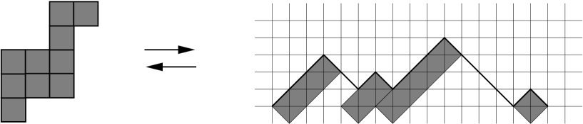
Figure 1: The set of staircase polygons is in one-to-one correspondence with the set of Dyck paths [11, 43]. Vertical column heights of a polygon correspond to peak heights of a path.

In turn, Dyck paths are classical objects of enumerative combinatorics [43], which are asymptotically described by Brownian excursions. This connection is described at various places in the literature, see e.g. [22, 44, 1]. Moreover, Dyck paths are closely related to models of trees [11, 43], as indicated in Figure 2.

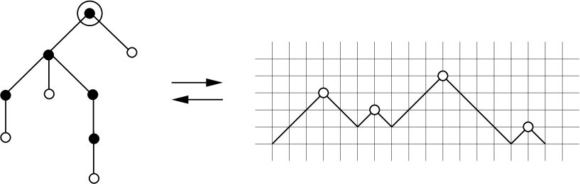
Figure 2: The set of rooted, ordered trees is in one-to-one correspondence with the set of Dyck paths [11, 43]. Leave distances to the root of a tree correspond to peak heights of a path.

In fact, the generating functions of polygon models, models of (simply generated) trees, and models of paths satisfy similar functional equations, typically leading to limit distributions of the same type. More generally, it appears that limit distributions for counting parameters are irrelevant of many details of the functional equation. This phenomenon of universality has recently been investigated using the setup of $q$-functional equations [41] and extends previous results [14, 38] by including counting parameters which generalise the polygon area. The results in [41] were obtained by an interplay between methods from statistical physics, combinatorics and stochastics. Corresponding counting parameters appeared previously within a combinatorial setup, see Duchon [14] and Nguy$\tilde{\mbox{\rm\^{e}}}$n Th$\acute{\mbox{\rm\^{e}}}$ [30, 31]. The derivation of moment recurrences of limit distributions for these parameters is inspired by the method of dominant balance as used by Prellberg and Brak [34] in polygon statistical physics, and some results for the corresponding stochastic objects appear to be unknown in the stochastics literature.

The outline of this article is as follows. We first derive a functional equation for the generating function of staircase polygons, counted by perimeter and sums of $k$-th powers of lengths of diagonals, $k$ being a positive integer. We also analyse a corresponding quantity for column heights. We then derive limit distributions for the above counting parameters in the limit of large perimeter, resp. width. We will first review the case $k=1$, which serves as a preparation for the following section, where the case of general $k$ is discussed. We then investigate the question of universality of our results by comparing them to Monte-Carlo simulations of self-avoiding polygons. The simulations indicate that the considered parameters have different laws for self-avoiding polygons and for staircase polygons. The methods discussed in this paper can be applied to similar problems concerning models of walks and models of trees. This we indicate for various models of discrete walks related to Dyck paths, such as meanders and bridges. The analysis extends previous work [30, 31], where mainly the case $k=2$ is studied.

2 Functional equations

Consider two fully directed walks on the edges of the square lattice (i.e., walks stepping only up or right), which both start at the origin and end in the same vertex, but have no other vertex in common. The edge set of such a configuration is called a staircase polygon, if it is nonempty. Each staircase polygon is a self-avoiding polygon. For a given staircase polygon, consider the construction of moving the upper directed walk one unit down and one unit to the right. For each walk, remove its first and its last edge. The resulting object is a sequence of (horizontal and vertical) edges and staircase polygons, see Figure 3. The unit square yields the empty sequence.

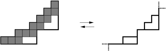
Figure 3: The set of staircase polygons is in one-to-one correspondence with the set of ordered sequences of edges and staircase polygons. A corresponding bijection is geometrically characterised by shifting the upper walk of a staircase polygon one unit down and one unit to the left, and by then removing the first and the last edge of each walk.

Using this construction, it is easy to see that the set of staircase polygons $\cal P$ is in one-to-one correspondence with the set $\cal Q$ of ordered sequences of edges and staircase polygons. Let us denote the corresponding map by $f:\cal P\to\cal Q$. Thus, for a staircase polygon $p\in\cal P$, we have $f(p)=(q_{1},\ldots,q_{n})\in\cal Q$, where $q_{i}$ is, for $i=1,\ldots,n$, either a single edge or a staircase polygon. The image of the unit square is the empty sequence $n=0$. A variant of this decomposition will be used below in order to derive a functional equation for the generating function of staircase polygons.

The horizontal (vertical) perimeter of a staircase polygon is the number of its horizontal (vertical) edges, its (total) perimeter is the sum of horizontal and vertical perimeter. The horizontal half-perimeter is also called the width of the polygon, the vertical half-perimeter is also called the height of the polygon. The area of a staircase polygon is the number of its enclosed squares. The half-perimeter of a staircase polygon is equal to the number of its (negative) diagonals plus one, the area of a staircase polygon equals the sum of the lengths of its (negative) diagonals, see Figure 4 for an illustration.

Figure 4: A staircase polygon of half-perimeter 14 and area 18. It has 8 diagonals of length one and 5 diagonals of length two.

For $k$ a nonnegative integer, we will consider $k$-th diagonal length moments of a staircase polygon $p$, defined by

$$n_{k}(p)=\sum_{d\in D(p)}l(d)^{k},$$ (2.1)

where the summation ranges over the set of diagonals $D(p)$ of $p$, with $l(d)$ denoting the length of $d$, i.e., the number of squares crossed by $d$. We count staircase polygons by half-perimeter $n_{0}(p)+1$ and by the parameters $n_{k}(p)$, where $k=1,\ldots,M$. Let $\boldsymbol{u}=(u_{0},\ldots,u_{M})$ denote formal variables. For a staircase polygon $p$, define its weight $w_{p}(\boldsymbol{u})$ by

$$w_{p}(\boldsymbol{u})=u_{0}^{n_{0}(p)+1}u_{1}^{n_{1}(p)}\cdot\ldots\cdot u_{M}^{n_{M}(p)},$$

and let $G(\boldsymbol{u})=\sum_{p\in\cal P}w_{p}(\boldsymbol{u})$ denote the generating function of $\cal P$. The bijection described above can be used to derive a functional equation for $G(\boldsymbol{u})$.

Theorem 2.1.

The generating function $G(\boldsymbol{u})$ of staircase polygons satisfies

$$G(\boldsymbol{u})=\frac{u_{0}^{2}u_{1}\cdot\ldots\cdot u_{M}}{1-2u_{0}\cdot\ldots\cdot u_{M}-G(\boldsymbol{v}(\boldsymbol{u}))},$$ (2.2)

where the functions $v_{k}({\boldsymbol{u}})$ are given by

$$v_{k}({\boldsymbol{u}})=\prod_{l=k}^{M}u_{l}^{\binom{l}{k}}\qquad(k=0,1,\ldots,M).$$ (2.3)

Proof.

For a sequence $q=(q_{1},\ldots q_{n})\in\cal Q$, its preimage $p=f^{-1}(q)\in\cal P$ can be described in the following way, which will prove more convenient for enumeration purposes. Consider the sequence $(p_{1},\ldots,p_{n})$ of staircase polygons, where $p_{i}=f^{-1}((q_{i}))$, for $i=1,\ldots,n$. The staircase polygon $p$ is obtained from $(p_{1},\ldots,p_{n})$ by concatenation, i.e., by translating $p_{i+1}$ such that the top right square of $p_{i}$ and the lower left square of $p_{i+1}$ coincide, for $i=1,\ldots,n-1$. Let us denote by $\widetilde{\cal P}\subset\cal P$ the subset of staircase polygons such that for each $p\in\widetilde{\cal P}$ we have $p=f^{-1}(q)$, where $q$ is either a single edge or a staircase polygon. The above description implies that the set of staircase polygons is in one-to-one correspondence to the set of concatenated ordered sequences of staircase polygons from $\widetilde{\cal P}$.

For a single edge $e$, the weight of the staircase polygon $f^{-1}(e)$ is given by $w_{f^{-1}(e)}(\boldsymbol{u})=u_{0}^{3}u_{1}^{2}\cdot\ldots\cdot u_{M}^{2}$. For a staircase polygon $p$, note that by the binomial theorem we have

$$n_{k}(f^{-1}(p))=\sum_{d\in D(f^{-1}(p))}l(d)^{k}=2+\sum_{d\in D(p)}(l(d)+1)^{k}=2+\sum_{i=0}^{k}\binom{k}{i}n_{i}(p).$$

This implies for the weights

$$\begin{split}w_{f^{-1}(p)}(\boldsymbol{u})&=u_{0}\prod_{l=0}^{M}u_{l}^{n_{l}(f^{-1}(p))}=u_{0}\prod_{l=0}^{M}\left(u_{l}^{2}\prod_{k=0}^{l}u_{l}^{\binom{l}{k}n_{k}(p)}\right)=u_{0}\left(\prod_{l=0}^{M}u_{l}^{2}\right)\left(\prod_{k=0}^{M}\prod_{l=k}^{M}u_{l}^{\binom{l}{k}n_{k}(p)}\right)\\ &=u_{0}^{2}\left(\prod_{l=1}^{M}u_{l}\right)\left(\prod_{l=0}^{M}u_{l}u_{l}^{n_{0}(p)}\right)\left(\prod_{k=1}^{M}\prod_{l=k}^{M}u_{l}^{\binom{l}{k}n_{k}(p)}\right)\\ &=u_{0}^{2}\left(\prod_{l=1}^{M}u_{l}\right)v_{0}(\boldsymbol{u})\prod_{k=0}^{M}v_{k}(\boldsymbol{u})^{n_{k}(p)}=u_{0}^{2}u_{1}\cdot\ldots\cdot u_{M}w_{p}(\boldsymbol{v}(\boldsymbol{u})),\end{split}$$

where the functions $v_{k}(\boldsymbol{u})$ are given by (2.3). For a sequence $(p_{1},\ldots,p_{n})$ of staircase polygons, denote their concatenation by $c(p_{1},\ldots,p_{n})$. We have $w_{c(p_{1},p_{2})}(\boldsymbol{u})=u_{0}^{-2}u_{1}^{-1}\cdot\ldots\cdot u_{M}^{-1}w_{p_{1}}(\boldsymbol{u})w_{p_{2}}(\boldsymbol{u})$, a monomial in $\boldsymbol{u}$, and thus

$$w_{c(p_{1},\ldots,p_{n})}(\boldsymbol{u})=\frac{1}{u_{0}^{2(n-1)}u_{1}^{n-1}\cdot\ldots\cdot u_{M}^{n-1}}w_{p_{1}}(\boldsymbol{u})\cdot\ldots\cdot w_{p_{n}}(\boldsymbol{u}).$$

The above bijection yields a functional equation for the generating function $G(\boldsymbol{u})$. We have

$$\begin{split}G(\boldsymbol{u})&=\sum_{n=0}^{\infty}\sum_{(p_{1},\ldots,p_{n})\in(\widetilde{\cal P})^{n}}w_{c(p_{1},\ldots,p_{n})}(\boldsymbol{u})\\ &=\sum_{n=0}^{\infty}u_{0}^{2}u_{1}\cdot\ldots\cdot u_{M}\sum_{(p_{1},\ldots,p_{n})\in(\widetilde{\cal P})^{n}}\frac{w_{p_{1}}(\boldsymbol{u})}{u_{0}^{2}u_{1}\cdot\ldots\cdot u_{M}}\cdot\ldots\cdot\frac{w_{p_{n}}(\boldsymbol{u})}{u_{0}^{2}u_{1}\cdot\ldots\cdot u_{M}}\\ &=u_{0}^{2}u_{1}\cdot\ldots\cdot u_{M}\sum_{n=0}^{\infty}\left(\frac{1}{u_{0}^{2}u_{1}\cdot\ldots\cdot u_{M}}\sum_{p\in\widetilde{\cal P}}w_{p}(\boldsymbol{u})\right)^{n}\\ &=u_{0}^{2}u_{1}\cdot\ldots\cdot u_{M}\frac{1}{1-\frac{1}{u_{0}^{2}u_{1}\cdot\ldots\cdot u_{M}}\left(2w_{f^{-1}(e)}(\boldsymbol{u})+\sum_{p\in\cal P}w_{f^{-1}(p)}(\boldsymbol{u})\right)}\\ &=\frac{u_{0}^{2}u_{1}\cdot\ldots\cdot u_{M}}{1-2u_{0}u_{1}\cdot\ldots\cdot u_{M}-G(\boldsymbol{v}(\boldsymbol{u}))}\end{split}$$

This is the functional equation (2.2). ∎

Remark. The case $M=0$ is standard, see e.g. [43]. The case $M=1$ has been studied by various techniques in [18, 11, 34, 7]. For corresponding models of walks and trees, see also the review in [17]. Analogous counting parameters for the case $M>1$ appear, within the context of wall polyominoes, in [14]. This study has been extended in [30, 31] and in [41]. Whereas the focus in [30, 31] is on particular examples of directed walks such as Dyck paths, [14] (resp. [41]) also discuss the structure of underlying classes of functional equations in the case $M=1$ (resp. $M>1$). Explicit expressions for the generating function $G(\boldsymbol{u})$ have been obtained for $M=0$ and $M=1$, see the above references. A functional equation for staircase polygons, counted by the above parameters and by width and height in addition (with formal variables $x$ and $y$), can be derived by the same method. It is obtained from (2.2) by multiplying the rhs with $xy$ and replacing the factor of two in the denominator by $(x+y)$.

Instead of considering diagonal length moments, one can also analyse $k$-th column height moments of a staircase polygon $p$, defined by $m_{k}(p)=\sum_{c\in C(p)}l(c)^{k}$, where the sum is over all (vertical) columns $c$ of $p$, with $C(p)$ denoting the set of (vertical) columns of $p$, and with $l(c)$ denoting the number of squares in column $c$. Obviously, $m_{0}(p)$ is the width, $m_{1}(p)$ the area of $p$. Counting polygons by column height moments, width and height $h(p)$ leads one to consider weights

$$\widetilde{w}_{p}(\boldsymbol{u},y)=y^{h(p)}\cdot u_{0}^{m_{0}(p)}\cdot\ldots\cdot u_{M}^{m_{M}(p)},$$

$y$ being a formal variable. Let $H(\boldsymbol{u},y)=\sum_{p\in\cal P}\widetilde{w}_{p}(\boldsymbol{u},y)$ denote the corresponding generating function. For a staircase polygon, consider the construction of moving the upper walk of the polygon one unit down, and removing its first edge and the last edge of the lower walk. Similarly to the case discussed above, this construction can be used to derive a functional equation for $H(\boldsymbol{u},y)$. It is

$$H(\boldsymbol{u},y)=y\frac{H(\boldsymbol{v}(\boldsymbol{u}),y)+u_{0}\cdot\ldots\cdot u_{M}}{1-(H(\boldsymbol{v}(\boldsymbol{u}),y)+u_{0}\cdot\ldots\cdot u_{M})},$$ (2.4)

where the functions $v_{k}({\boldsymbol{u}})$ are again given by (2.3).

Consider now the problem of counting staircase polygons by (total) half-perimeter and by column height moments. The generating function of the model is given by $H(\boldsymbol{u},u_{0})$. Since the sum of column heights of a staircase polygon is its area, for $M=1$ we have $H(u_{0},u_{1},u_{0})=G(u_{0},u_{1})$ with functional equation (2.2). For $M>1$, the diagonal moment approach for deriving a functional equation cannot be adapted to the present case, since in the inflation step, which includes the addition of a vertical layer, the height of a column may be increased by more than one unit. It is not possible to keep track of this varying height increase without introducing new auxiliary variables in the generating function. But then, the method of extracting limit distributions of section 4 cannot be applied in its present form. Since we prefer a model where limit distributions are considered with respect to large perimeter (and not to large width), we chose to discuss the diagonal length moment model. However, this choice is no restriction, since limit distributions of the first two models are of the same type, see section 4. Also, an exact analysis of the first few moments of the third model suggests the same type of limit distribution, see section 5 below.

3 Perimeter and area generating function

In this section, we will review the case $M=1$, which corresponds to counting polygons by half-perimeter and area. Whereas most results discussed below have appeared at various places in the literature [34, 14, 17, 37, 38], we recollect them here informally in order to prepare for the following section, where the case of general $M$ is discussed.

Consider the functional equation (2.2) for $M=1$ and set $u_{0}=t$ and $u_{1}=q$. The generating function $G(t,q)$ of staircase polygons, counted by half-perimeter and area, satisfies the functional equation

$$G(t,q)=\frac{t^{2}q}{1-2tq-G(tq,q)}.$$ (3.1)

The function $G(t):=G(t,1)$ is the generating function for staircase polygons counted by half-perimeter. If $q=1$, the functional equation (3.1) reduces to a quadratic equation, whose relevant solution is given by

$$\begin{split}G(t)&=\frac{1-2t-\sqrt{1-4t}}{2}=\sum_{n=1}^{\infty}\frac{1}{n+1}\binom{2n}{n}t^{n+1}=t^{2}+2t^{3}+5t^{4}+14t^{5}+{\cal O}(t^{6}),\end{split}$$

where $C_{n}=\binom{2n}{n}/(n+1)$ is the $n$-th Catalan number. Thus, the number $p_{n}$ of staircase polygons of half-perimeter $n$ is given by

$$p_{n}=C_{n-1}=\frac{1}{n}\binom{2n-2}{n-1}=\frac{1}{\sqrt{\pi}}\frac{4^{n-1}}{n^{3/2}}\left(1+{\cal O}(n^{-1})\right).$$

The above asymptotic form for $p_{n}$ can alternatively be obtained by singularity analysis of the generating function $G(t)$. Such an approach will also be used in the following section. The function $t\mapsto G(t)$ is analytic for $|t|\leq t_{c}=1/4$ except at $t=t_{c}$. The above expression yields an expansion about $t=t_{c}$ of the form

$$G(t)=G(t_{c})+\sum_{l=0}^{\infty}f_{0,l}(t_{c}-t)^{(l+1)/2},$$ (3.2)

where $G(t_{c})=1/4$, $f_{0,0}=-1$, $f_{0,1}=1$, and $f_{0,l}=0$ for $l>1$. In order to obtain information about the coefficients of $G(t)$, we remind that functions $g(x)=(x_{c}-x)^{-\gamma}$ with rational exponent $\gamma\notin\{-1,-2,\ldots\}$ satisfy

$$[x^{n}]g(x)=\frac{1}{x_{c}^{\gamma}\Gamma(\gamma)}x_{c}^{-n}n^{\gamma-1}\left(1+{\cal O}(n^{-1})\right),$$ (3.3)

where $[x^{n}]f(x)$ denotes the coefficient of order $n$ in the power series $f(x)$, and $\Gamma(z)$ denotes the Gamma function [16, 42]. Applying this result to the (finite) expansion (3.2) yields the above asymptotic form for $p_{n}$.

We are interested in a probabilistic description of staircase polygons. Let ${\cal P}_{n}\subset\cal P$ denote the subset of staircase polygons of half-perimeter $n$. Consider a uniform model, where each polygon $p\in{\cal P}_{n}$ occurs with equal probability. We ask for the mean area of a polygon of half-perimeter $n$. To this end, introduce a discrete random variable $\widetilde{X}_{n}$ of polygon area by

$$\mathbb{P}(\widetilde{X}_{n}=m)=\frac{p_{n,m}}{\sum_{m}p_{n,m}},$$

where $p_{n,m}$ denotes the number of polygons of half-perimeter $n$ and area $m$. Note that the numbers $p_{n,m}$ appear in the expansion $G(t,q)=\sum_{n,m}p_{n,m}t^{n}q^{m}$ of the perimeter and area generating function $G(t,q)$. The mean area of a staircase polygon of half-perimeter $n$ is then given by

$$\mathbb{E}[\widetilde{X}_{n}]=\frac{\sum_{m}mp_{n,m}}{\sum_{m}p_{n,m}}=\frac{[t^{n}]\left.q\frac{\partial}{\partial q}G(t,q)\right|_{q=1}}{[t^{n}]G(t,1)}.$$

The function appearing in the numerator can be obtained from the functional equation (3.1) by differentiating w.r.t. $q$ and setting $q=1$. This yields $\left.\frac{\partial}{\partial q}G(t,q)\right|_{q=1}=t^{2}/(1-4t)$, and we get

$$\mathbb{E}[\widetilde{X}_{n}]=\frac{4^{n-2}}{C_{n-1}}=\frac{\sqrt{\pi}}{4}n^{3/2}\left(1+{\cal O}(n^{-1})\right).$$

Thus, the mean area of a staircase polygon scales with its perimeter as $n^{3/2}$. For a single staircase polygon, the mean length of its diagonals is given by the quotient of area and half-perimeter $n$ minus one. Thus, the mean length of a diagonal of a random staircase polygon scales with its perimeter as $n^{1/2}$. The mean width of a staircase polygon may be analysed similarly using the width and height generating function, which is algebraic of degree two, see (2.4). It can be shown that the mean width of a staircase polygon scales with its perimeter as $n$. Also, it can be shown that the mean column height of a staircase polygon scales with its perimeter (width) as $n^{1/2}$.

Higher moments of the area random variable $\widetilde{X}_{n}$ can be computed similarly to the discussion above. For the $k$-th factorial moment of $\widetilde{X}_{n}$, where $k\in\mathbb{N}$, we have

$$\mathbb{E}[(\widetilde{X}_{n})_{k}]=\frac{\sum_{m}(m)_{k}p_{n,m}}{\sum_{m}p_{n,m}}=\frac{[t^{n}]\left.\frac{\partial^{k}}{\partial q^{k}}G(t,q)\right|_{q=1}}{[t^{n}]G(t,1)},$$ (3.4)

where $(a)_{k}=a(a-1)\cdot\ldots\cdot(a-k+1)$. Derivatives of $G(t,q)$ can be obtained recursively from the functional equation (3.1) by repeated differentiation w.r.t. $q$. The result (see Lemma 4.1 in the next section) is given a follows. The derivative in (3.4) is algebraic, with leading singular behaviour

$$\frac{1}{k!}\left.\frac{\partial^{k}}{\partial q^{k}}G(t,q)\right|_{q=1}=\frac{f_{k}}{(t_{c}-t)^{\gamma_{k}}}\left(1+{\cal O}((t_{c}-t)^{1/2})\right),$$ (3.5)

where $\gamma_{k}=3k/2-1/2$, and $f_{k}$ (strictly) positive. A recursion for the coefficient $f_{k}$ is given by

$$\frac{1}{16}\gamma_{k-1}f_{k-1}+\sum_{0\leq l\leq k}f_{l}f_{k-l}=0,$$ (3.6)

where $k\in\mathbb{N}$ and $f_{0}=-1$. Inserting (3.5) into (3.4) and extracting coefficients, using (3.3) and standard transfer theorems [16], gives

$$\mathbb{E}[(\widetilde{X}_{n})_{k}]=\frac{k!}{f_{0}t_{c}^{\gamma_{k}-\gamma_{0}}}\frac{\Gamma(\gamma_{0})}{\Gamma(\gamma_{k})}f_{k}n^{3k/2}\left(1+{\cal O}(n^{-1/2})\right).$$

The (factorial) moments of $\widetilde{X}_{n}$ diverge for large perimeter. In order to obtain a limit distribution, we introduce a normalised random variable $X_{n}$ of area by setting $X_{n}=\widetilde{X}_{n}/n^{3/2}$. This normalisation is natural in view of the scaling of the mean area with the perimeter, as described above. Alternatively, the area is the sum over diagonal lengths (column heights) and thus scales like $n\cdot n^{1/2}$, as argued above. The moments of $X_{n}$ are then asymptotically given by

$$\mathbb{E}[X_{n}^{k}]=\mathbb{E}[(X_{n})_{k}]\left(1+{\cal O}(n^{-1/2})\right)=\frac{k!}{f_{0}t_{c}^{\gamma_{k}-\gamma_{0}}}\frac{\Gamma(\gamma_{0})}{\Gamma(\gamma_{k})}f_{k}\left(1+{\cal O}(n^{-1/2})\right),$$

where we expressed the $k$-th moments in terms of the $r$-th factorial moments, $r=0,1,\ldots,k$. The recursion (3.6) can be used to show that the values $m_{k}=\lim_{n\to\infty}\mathbb{E}[X_{n}^{k}]$ satisfy the Carleman condition $\sum_{k}(m_{k})^{-1/k}=+\infty$, implying the existence and uniqueness of a limit distribution with moments $m_{k}$ [5]. This distribution is known as the Airy distribution, see [17] for a review. For models of simply generated trees, corresponding convergence results appear in [1, 13].

We finally describe a convenient technique to compute the numbers $f_{k}$, which will be central in the following sections. This approach, called the method of dominant balance [34], was initially followed when analysing the scaling function of staircase polygons [37]. Whereas it has been applied under a certain analyticity assumption on the corresponding model, it can be given a rigorous meaning at a formal level, see the remark after Lemma 4.1 in the following section. It has been proved [33, Thm. 5.3] that there exists a uniform asymptotic expansion of the perimeter and area generating function $G(t,q)$ about $t=t_{c}$, which is, to leading order, given by

$$G(t,q)\sim G(t_{c})+(t_{c}-t)^{1/2}F_{0}\left(\frac{1-q}{(t_{c}-t)^{3/2}}\right)\qquad(t\to t_{c}^{-}),$$ (3.7)

uniformly in $q\leq 1$ near unity. The function $F_{0}(\epsilon)$ is called the scaling function and admits an asymptotic expansion about $\epsilon=0$, the exponents $1/2$ and $3/2$ are called the critical exponents of the model, see also [34, 33, 19]. The scaling function is explicitly given by

$$F_{0}(\epsilon)=\epsilon^{1/3}\frac{2^{-4/3}\mbox{Ai}^{\prime}(2^{8/3}\epsilon^{-2/3})}{\mbox{Ai}(2^{8/3}\epsilon^{-2/3})}=-1-\frac{1}{64}\epsilon+\frac{5}{8192}\epsilon^{2}-\frac{15}{262144}\epsilon^{3}+{\cal O}(\epsilon^{4}),$$

where $\mbox{Ai}(z)=\frac{1}{\pi}\int_{0}^{\infty}\cos(t^{3}/3+tz){\rm d}t$ is the Airy function. The coefficients $f_{k}$ of (3.5) appear in the scaling function via $F_{0}(\epsilon)=\sum_{k\geq 0}(-1)^{k}f_{k}\epsilon^{k}$. This is seen by asymptotically evaluating the lhs of (3.5), using the scaling form (3.7), and by comparing to the rhs of (3.5). The scaling function can be extracted from the functional equation (3.1) as follows. Insert the scaling form (3.7) for the generating function $G(t,q)$ in the functional equation (3.1) and introduce new variables $s$ and $\epsilon$ by setting $x=x_{c}-s^{2}$ and $q=1-\epsilon s^{3}$. Then, the functional equation yields a differential equation for $F_{0}(\epsilon)$, when expanded up to order $s^{2}$, see also [38] for a detailed account. The differential equation for $F_{0}(\epsilon)$ is of Riccati type and given by

$$\frac{1}{16}\epsilon\left(\frac{1}{2}F_{0}(\epsilon)-\frac{3}{2}\epsilon F_{0}^{\prime}(\epsilon)\right)+F_{0}(\epsilon)^{2}=1.$$

This immediately translates into the above recursion (3.6) for the coefficients $f_{k}$ of the scaling function.

4 Limit distributions and scaling functions

We now consider the case of arbitrary $M$. Whereas this leads to cumbersome expressions, we are following the same ideas as in the previous section. Recall that the set of staircase polygons of half-perimeter $n_{0}$ is denoted by ${\cal P}_{n_{0}}$. We consider a uniform model where each polygon $p\in{\cal P}_{n_{0}}$ occurs with equal probability. Then, to each counting parameter a corresponding random variable is attached. This leads us to consider discrete random variables $\widetilde{X}_{k,n_{0}}$ for the diagonal length moments $n_{k}(p)$, for $k=1,\ldots,M$. The generating function $G(\boldsymbol{u})$ is a formal power series in $\boldsymbol{u}$, i.e., $G(\boldsymbol{u})\in\mathbb{C}[[\boldsymbol{u}]]$, where $R[[x_{1},\ldots,x_{N}]]$ denotes the ring of formal $R$-power series in the variables $x_{1},\ldots,x_{N}$. In fact, $G(\boldsymbol{u})\in\mathbb{Z}[u_{1},\ldots,u_{M}][[u_{0}]]$, where $R[x_{1},\ldots,x_{N}]$ denotes the ring of $R$-polynomials in the variables $x_{1},\ldots,x_{N}$. The function $G(\boldsymbol{u}_{0})$, where $\boldsymbol{u}_{0}=(u_{0},1,\ldots,1)$, as considered in the previous section, is the (half-) perimeter generating function of the model. Write the generating function $G(\boldsymbol{u})$ as

$$G(\boldsymbol{u})=\sum_{n_{0},n_{1},\ldots,n_{M}}p_{n_{0},n_{1},\ldots,n_{M}}u_{0}^{n_{0}}u_{1}^{n_{1}}\cdot\ldots\cdot u_{M}^{n_{M}}.$$

The coefficient $p_{n_{0},n_{1},\ldots,n_{M}}$ is the number of staircase polygons of half-perimeter $n_{0}$ where, for $k=1,\ldots,M$, the $k$-th diagonal length moment has the value $n_{k}$. We have $0<\sum_{n_{1},\ldots,n_{M}}p_{n_{0},n_{1},\ldots,n_{M}}=[u_{0}^{n_{0}}]G(\boldsymbol{u}_{0})=C_{n_{0}-1}<\infty$, where $C_{n}$ is the $n$-th Catalan number. In a uniform model, where each polygon $p\in{\cal P}_{n_{0}}$ has the same probability $1/C_{n_{0}-1}$, the discrete random variables $\widetilde{X}_{k,n_{0}}$ corresponding to the diagonal moments $n_{k}(p)$ have the probability distribution

$$\mathbb{P}(\widetilde{X}_{1,n_{0}}=n_{1},\ldots,\widetilde{X}_{M,n_{0}}=n_{M})=\frac{p_{n_{0},n_{1},\ldots,n_{M}}}{\sum_{n_{1},\ldots,n_{M}}p_{n_{0},n_{1},\ldots,n_{M}}}.$$

We will analyse the joint distribution of the random variables $\widetilde{X}_{k,n_{0}}$, where $k=1,\ldots,M$, in the limit of large perimeter. This will be achieved by studying asymptotic properties of mixed moments of the random variables $\widetilde{X}_{k,n_{0}}$, given by

$$\mathbb{E}[\widetilde{X}_{1,n_{0}}^{k_{1}}\cdot\ldots\cdot\widetilde{X}_{M,n_{0}}^{k_{M}}]=\frac{\sum_{n_{1},\ldots,n_{M}}n_{1}^{k_{1}}\cdot\ldots\cdot n_{M}^{k_{M}}p_{n_{0},n_{1},\ldots,n_{M}}}{\sum_{n_{1},\ldots,n_{M}}p_{n_{0},n_{1},\ldots,n_{M}}}.$$

We employ a generating function method. Note that we have

$$\mathbb{E}[\widetilde{X}_{1,n_{0}}^{k_{1}}\cdot\ldots\cdot\widetilde{X}_{M,n_{0}}^{k_{M}}]=\frac{[u_{0}^{n_{0}}]\left.\left(u_{1}\frac{\partial}{\partial u_{1}}\right)^{k_{1}}\cdot\ldots\cdot\left(u_{M}\frac{\partial}{\partial u_{M}}\right)^{k_{M}}G(\boldsymbol{u})\right|_{\boldsymbol{u}=\boldsymbol{u}_{0}}}{[u_{0}^{n_{0}}]G(\boldsymbol{u}_{0})}.$$

We can thus study asymptotic properties of the moments by studying asymptotic properties of the coefficients of the generating functions appearing on the rhs of the above equation. The latter problem can be treated by singularity analysis of generating functions, as indicated in the previous section. It will prove convenient to consider factorial moments, given by

$$\mathbb{E}[(\widetilde{X}_{1,n_{0}})_{k_{1}}\cdot\ldots\cdot(\widetilde{X}_{M,n_{0}})_{k_{M}}]=\frac{[u_{0}^{n_{0}}]\left.\frac{\partial^{k_{1}}}{\partial u_{1}^{k_{1}}}\cdot\ldots\cdot\frac{\partial^{k_{M}}}{\partial u_{M}^{k_{M}}}G(\boldsymbol{u})\right|_{\boldsymbol{u}=\boldsymbol{u}_{0}}}{[u_{0}^{n_{0}}]G(\boldsymbol{u}_{0})}.$$

Moments can be expressed linearly in factorial moments. It will turn out below that they are, for $k_{1},\ldots,k_{M}$ fixed, asymptotically equal. Let us introduce factorial moment generating functions $g_{\boldsymbol{k}}(u_{0})$, defined by

$$g_{\boldsymbol{k}}(u_{0}):=\left.\frac{1}{\boldsymbol{k}!}\frac{\partial^{k_{1}}}{\partial u_{1}^{k_{1}}}\cdots\frac{\partial^{k_{M}}}{\partial u_{M}^{k_{M}}}G(\boldsymbol{u})\right|_{\boldsymbol{u}=\boldsymbol{u}_{0}},$$

where $\boldsymbol{k}=(k_{1},\ldots,k_{M})\in\mathbb{N}_{0}^{M}$. We use the multi-index notation. In particular, $\boldsymbol{k}!=k_{1}!\cdot\ldots\cdot k_{M}!$, $|\boldsymbol{k}|=k_{1}+\ldots+k_{M}$, and $\boldsymbol{k}\leq\boldsymbol{l}$ if $k_{i}\leq l_{i}$ for $i=1,\ldots,M$. We will also use unit vectors $\boldsymbol{e}_{k}$, $k=1,\ldots,M$, with coordinates $(e_{k})_{i}=\delta_{i,k}$ for $i=1,\ldots,M$. We clearly have $g_{\boldsymbol{k}}(u_{0})\in\mathbb{C}[[u_{0}]]$ for all $\boldsymbol{k}$. The function $g_{\boldsymbol{0}}(u_{0})=G(\boldsymbol{u}_{0})=G(u_{c})+\sum_{l=0}^{\infty}f_{\boldsymbol{0},l}(u_{c}-u_{0})^{(l+1)/2}$ has been studied in the previous section (3.2), where we found $u_{c}=1/4$, $G(u_{c})=1/4$, $f_{\boldsymbol{0},0}=-1$, $f_{\boldsymbol{0},1}=1$, and $f_{\boldsymbol{0},l}=0$ for $l>1$. The functional equation (2.2) can be used to show that the properties of $g_{\boldsymbol{0}}(u_{0})$ carry over to those of $g_{\boldsymbol{k}}(u_{0})$ for $\boldsymbol{k}\neq\boldsymbol{0}$. We have the following lemma.

Lemma 4.1.

For $\boldsymbol{k}\neq\boldsymbol{0}$, all factorial moment generating functions $g_{\boldsymbol{k}}(u_{0})$ are algebraic. They are analytic for $|u_{0}|\leq u_{c}=1/4$, except at $u_{0}=u_{c}$, with Puiseux expansions of the form

$$g_{\boldsymbol{k}}(u_{0})=\sum_{l=0}^{\infty}f_{\boldsymbol{k},l}(u_{c}-u_{0})^{l/2-\gamma_{\boldsymbol{k}}},$$ (4.1)

where $\gamma_{\boldsymbol{k}}=-1/2+\sum_{i=1}^{M}(1+i/2)k_{i}$. The leading coefficients $f_{\boldsymbol{k},0}=f_{\boldsymbol{k}}$ are given by $f_{\boldsymbol{k}}=c_{\boldsymbol{k}}f_{\boldsymbol{0}}^{1-|\boldsymbol{k}|}f_{\boldsymbol{e}_{1}}^{k_{1}}\cdot\ldots\cdot f_{\boldsymbol{e}_{M}}^{k_{M}}$, where the numbers $c_{\boldsymbol{k}}$ are, for $\boldsymbol{k}\neq\boldsymbol{0}$, determined by the recursion

$$c_{\boldsymbol{k}}=-2\gamma_{{\boldsymbol{k}}-{\boldsymbol{e}}_{1}}c_{{\boldsymbol{k}}-{\boldsymbol{e}}_{1}}+\sum_{i=1}^{M-1}(k_{i}+1)c_{{\boldsymbol{k}}-{\boldsymbol{e}}_{i+1}+{\boldsymbol{e}}_{i}}-\frac{1}{2}\sum_{\begin{subarray}{c}{\boldsymbol{l}}\neq{\bf 0},{\boldsymbol{l}}\neq{\boldsymbol{k}}\\ {\bf 0}\leq{\boldsymbol{l}}\leq{\boldsymbol{k}}\end{subarray}}c_{\boldsymbol{l}}c_{{\boldsymbol{k}}-{\boldsymbol{l}}},$$ (4.2)

with boundary conditions $c_{\boldsymbol{0}}=1$ and $c_{\boldsymbol{k}}=0$ if $k_{j}<0$ for some $1\leq j\leq M$. The coefficients $f_{\boldsymbol{k}}$ are strictly positive for ${\boldsymbol{k}}\neq{\bf 0}$. Explicitly, we have $f_{\boldsymbol{0}}=-1$ and $f_{\boldsymbol{e}_{k}}=k!2^{-3(k+1)}$ for $k=1,\ldots,M$.

Proof.

The above lemma is a special case of [41, Prop. 5.3, 5.6]. We outline the idea of proof.

Successively differentiating the functional equation (2.2) yields $g_{\boldsymbol{k}}(u_{0})$ as rational function of $g_{\boldsymbol{0}}(u_{0})$ and its derivatives. Due to the closure properties of algebraic functions, these functions are algebraic again. The functions $g_{\boldsymbol{k}}(u_{0})$ then inherit analytic properties of $g_{\boldsymbol{0}}(u_{0})$. In particular, $g_{\boldsymbol{k}}(u_{0})$ is analytic for $|u_{0}|\leq u_{c}$, except at $u_{0}=u_{c}$, with a Puiseux expansion of the form (4.1) for some exponent $\widetilde{\gamma}_{\boldsymbol{k}}$. The value of the leading exponent $\gamma_{\boldsymbol{k}}$ and the recursion for the coefficients $f_{\boldsymbol{k}}$ (hence for the coefficients $c_{\boldsymbol{k}}$) is proved by induction, via asymptotically analysing the $\boldsymbol{k}$-th derivative of the functional equation. ∎

Remarks.
i) For the model (2.4) of staircase polygons, counted by width and (vertical) column height moments, Lemma 4.1 applies as well, however with different numbers $u_{c}=(1-\sqrt{y})^{2}$ for $0<y<1$, $f_{\boldsymbol{0}}=-y^{-1/4}$ and $f_{\boldsymbol{e}_{k}}=k!2^{-k}y^{-k/4}$ for $k=1,\ldots,M$. It has been shown that Lemma 4.1 applies in a much more general context [41, Prop. 5.6]. In particular, the amplitude ratios $f_{\boldsymbol{k}}f_{\boldsymbol{0}}^{|\boldsymbol{k}|-1}f_{\boldsymbol{e}_{1}}^{-k_{1}}\cdot\ldots\cdot f_{\boldsymbol{e}_{M}}^{-k_{M}}=c_{\boldsymbol{k}}$ are model independent in that situation, i.e., independent of $u_{c}$, $f_{\boldsymbol{0}}$ and $f_{\boldsymbol{e}_{k}}$.
ii) The recursion (4.2) for the coefficients $f_{\boldsymbol{k}}$ can be obtained mechanically, if a tight bound on the exponents $\gamma_{\boldsymbol{k}}$ is known. (Typically, analysis of the first few functions $g_{\boldsymbol{k}}(u_{0})$ suggests the form of $\gamma_{\boldsymbol{k}}$. Then, one can prove that $\gamma_{\boldsymbol{k}}$ is an exponent bound by induction, using the functional equation. Such a proof is generally easier than a full asymptotic analysis of the functional equation, see [41, Prop. 5.5].) If we replace the functions $g_{\boldsymbol{k}}(u_{0})$ in the expansion of $G(\boldsymbol{u})$ about $u_{1}=\ldots=u_{M}=1$ by their Puiseux expansions (4.1), we then have

$$\begin{split}G(\boldsymbol{u})&=\sum_{\boldsymbol{k}}(-1)^{|\boldsymbol{k}|}g_{\boldsymbol{k}}(u_{0})(1-u_{1})^{k_{1}}\cdot\ldots\cdot(1-u_{M})^{k_{M}}\\ &=G(u_{c})+\sqrt{u_{c}-u_{0}}F\left(\frac{1-u_{1}}{(u_{c}-u_{0})^{(1+2)/2}},\ldots,\frac{1-u_{M}}{(u_{c}-u_{0})^{(M+2)/2}},\sqrt{u_{c}-u_{0}}\right),\end{split}$$ (4.3)

where, for $\boldsymbol{\epsilon}=(\epsilon_{1},\ldots,\epsilon_{M})$, the function $F(\boldsymbol{\epsilon},s)\in\mathbb{C}[[\boldsymbol{\epsilon},s]]$ is a formal power series, and $F(\boldsymbol{\epsilon},s)=\sum_{l}F_{l}(\boldsymbol{\epsilon})s^{l}$, where $F_{l}(\boldsymbol{\epsilon})=\sum_{\boldsymbol{k}}(-1)^{|\boldsymbol{k}|}f_{\boldsymbol{k},l}\boldsymbol{\epsilon}^{\boldsymbol{k}}$. In statistical mechanics, the function $F_{0}(\boldsymbol{\epsilon})$ is called the scaling function, and the functions $F_{l}(\boldsymbol{\epsilon})$ are called the correction-to-scaling functions, if the equation (4.3) is valid as an asymptotic expansion in $u_{c}-u_{0}$, uniformly in $1-q_{1},\ldots,1-q_{M}$, see [19]. For a probabilistic interpretation, see the remark after Theorem 4.2.

The functional equation (2.2) induces partial differential equations for the functions $F_{l}(\boldsymbol{\epsilon})$. They are obtained by substituting (4.3) in (2.2), and by introducing variables $s,\epsilon_{1},\ldots,\epsilon_{M}$ via $u_{0}=u_{c}-s^{2}$ and $u_{k}=1-\epsilon_{k}s^{k+2}$ for $k=1,\ldots,M$. Then, a partial differential equation for $F_{l}(\boldsymbol{\epsilon})$ appears in the expansion of the functional equation in $s$ at order $s^{l+2}$. Computing these equations is called the method of dominant balance [34], see [38] for the case $M=1$, and [41] for the case of general $M$. For example, we get for $F_{0}(\boldsymbol{\epsilon})$ the equation

$$\frac{1}{16}\epsilon_{1}\left(\frac{1}{2}F_{0}(\boldsymbol{\epsilon})-\sum_{i=1}^{M}\left(1+\frac{i}{2}\right)\epsilon_{i}\frac{\partial F_{0}}{\partial\epsilon_{i}}(\boldsymbol{\epsilon})\right)+\sum_{i=1}^{M-1}\frac{(i+1)}{4}\epsilon_{i+1}\frac{\partial F_{0}}{\partial\epsilon_{i}}(\boldsymbol{\epsilon})+F_{0}(\boldsymbol{\epsilon})^{2}=1.$$ (4.4)

This yields, for $\boldsymbol{k}\neq\boldsymbol{0}$, a recursion for the coefficients $f_{\boldsymbol{k}}$ of $F_{0}(\boldsymbol{\epsilon})$ of the form

$$\frac{1}{16}\gamma_{{\boldsymbol{k}}-{\boldsymbol{e}}_{1}}f_{{\boldsymbol{k}}-{\boldsymbol{e}}_{1}}+\sum_{i=1}^{M-1}\frac{i+1}{4}(k_{i}+1)f_{{\boldsymbol{k}}-{\boldsymbol{e}}_{i+1}+{\boldsymbol{e}}_{i}}+\sum_{\bf 0\leq{\boldsymbol{l}}\leq{\boldsymbol{k}}}f_{\boldsymbol{l}}f_{{\boldsymbol{k}}-{\boldsymbol{l}}}=0,$$

which translates into the above recursion (4.2) for the coefficients $c_{\boldsymbol{k}}$.

We are now prepared for a discussion of moment asymptotics. Recall that the random variables $\widetilde{X}_{k,n_{0}}$ are related to the diagonal height moments $n_{k}(p)$, which are defined in (2.1). Since the number of diagonals of a staircase polygon equals its half-perimeter minus one, and the average diagonal length of a staircase polygon scales like $n_{0}^{1/2}$, we expect that the mean $k$-th diagonal length moment scales like $n_{0}^{1+k/2}$. We thus introduce normalised random variables $X_{k,n_{0}}$ by

$$(X_{1,n_{0}},X_{2,n_{0}},\ldots,X_{M,n_{0}})=\left(\frac{\widetilde{X}_{1,n_{0}}}{n_{0}^{3/2}},\frac{\widetilde{X}_{2,n_{0}}}{n_{0}^{4/2}},\ldots,\frac{\widetilde{X}_{M,n_{0}}}{n_{0}^{(M+2)/2}}\right).$$ (4.5)

Then, the mixed moments of the random variables $X_{k,n_{0}}$ converge to a finite, nonzero limit as $n_{0}\to\infty$. We have the following result.

Theorem 4.2.

The random variable $(X_{1,n_{0}},X_{2,n_{0}},\ldots,X_{M,n_{0}})$ of eqn. (4.5) converges in distribution,

$$(X_{1,n_{0}},X_{2,n_{0}},\ldots,X_{M,n_{0}})\stackrel{{\scriptstyle d}}{{\to}}(\alpha_{1}X_{1},\ldots,\alpha_{M}X_{M}),$$

where $X_{k}=\int e^{k}(t)\,{\rm d}t$ denotes the integral of the $k$-th power of the standard Brownian excursion of duration $1$, and the numbers $\alpha_{k}$ are given by $\alpha_{k}=-\frac{f_{\boldsymbol{e}_{k}}}{f_{\boldsymbol{0}}}\frac{2^{3-3k/2}}{k!}$. We also have moment convergence with

$$\mathbb{E}[X_{1,n_{0}}^{k_{1}}\cdot\ldots\cdot X_{M,n_{0}}^{k_{M}}]=\frac{\boldsymbol{k}!}{f_{\bf 0}u_{c}^{\gamma_{\boldsymbol{k}}-\gamma_{\bf 0}}}\frac{\Gamma(\gamma_{\boldsymbol{0}})}{\Gamma(\gamma_{\boldsymbol{k}})}f_{\boldsymbol{k}}\left(1+{\cal O}(n_{0}^{-1/2})\right),$$

where the numbers $u_{c}$, $\gamma_{\boldsymbol{k}}$ and $f_{\boldsymbol{k}}$ are those of Lemma 4.1. The numbers $\alpha_{k}$ are explicitly given by $\alpha_{k}=2^{-9k/2}$.

Proof.

Theorem 4.2 is obtained by specialising [41, Thm. 8.5] and [41, Cor. 9.1] to the functional equation (2.2). We sketch the proof.

By standard transfer theorems [16] for algebraic functions, the results of Lemma 4.1 translate to an asymptotic expression for the factorial moments. It is

$$\mathbb{E}[(\widetilde{X}_{1,n_{0}})_{k_{1}}\cdot\ldots\cdot(\widetilde{X}_{M,n_{0}})_{k_{M}}]=\frac{{\boldsymbol{k}}!}{f_{\bf 0}u_{c}^{\gamma_{\boldsymbol{k}}-\gamma_{\bf 0}}}\frac{\Gamma(\gamma_{\bf 0})}{\Gamma(\gamma_{\boldsymbol{k}})}f_{\boldsymbol{k}}n_{0}^{\gamma_{\boldsymbol{k}}-\gamma_{\bf 0}}+{\cal O}(n_{0}^{\gamma_{\boldsymbol{k}}-\gamma_{\bf 0}-1/2}),$$

The explicit error term implies that factorial moments are asymptotically equal to the (ordinary) moments $\mathbb{E}[\widetilde{X}_{1,n_{0}}^{k_{1}}\cdot\ldots\cdot\widetilde{X}_{M,n_{0}}^{k_{M}}]$. In particular, the moments $\mathbb{E}[X_{1,n_{0}}^{k_{1}}\cdot\ldots\cdot X_{M,n_{0}}^{k_{M}}]$ converge to a finite, nonzero limit as $n_{0}\to\infty$. We have

$$\mathbb{E}[X_{1,n_{0}}^{k_{1}}\cdot\ldots\cdot X_{M,n_{0}}^{k_{M}}]=\frac{\mathbb{E}[\widetilde{X}_{1,n_{0}}^{k_{1}}\cdot\ldots\cdot\widetilde{X}_{M,n_{0}}^{k_{M}}]}{n_{0}^{\gamma_{\boldsymbol{k}}-\gamma_{\bf 0}}}=\frac{{\boldsymbol{k}}!}{f_{\bf 0}u_{c}^{\gamma_{\boldsymbol{k}}-\gamma_{\bf 0}}}\frac{\Gamma(\gamma_{\bf 0})}{\Gamma(\gamma_{\boldsymbol{k}})}f_{\boldsymbol{k}}\left(1+{\cal O}(n_{0}^{-1/2})\right).$$

Set $m_{\boldsymbol{k}}=\lim_{n_{0}\to\infty}\mathbb{E}[X_{1,n_{0}}^{k_{1}}\cdot\ldots\cdot X_{M,n_{0}}^{k_{M}}]$. The recursion (4.2) or the partial differential equation (4.4) induces an upper bound on the growth of the coefficients $f_{\boldsymbol{k}}$. This can be used to show that for $\boldsymbol{t}\in\mathbb{R}^{M}$

$$\lim_{|\boldsymbol{k}|\to\infty}\frac{m_{\boldsymbol{k}}\boldsymbol{t}^{\boldsymbol{k}}}{\boldsymbol{k}!}=0.$$

This guarantees the existence and uniqueness of a limit distribution with moments $m_{\boldsymbol{k}}$ via Lévy’s continuity theorem [3]. The connection to Brownian excursions follows by comparing the moments, see [41, Thm. 2.4]. ∎

Remarks.
i) For a discussion of the case $M=1$, see the previous section. The case $M=2$ has been analysed in [30, 31]. The above approach yields the existence and uniqueness of a (joint) limit distribution for $M$ arbitrary, and provides recurrences for their mixed moments. It also allows to analyse corrections to the limiting behaviour. It applies in a more general setup of models whose generating function satisfy a $q$-functional equation [41]. This includes simply generated trees as a special case [1, 13]. For $M=1$ and $M=2$, moment recurrences for Dyck paths have also been obtained [31] via Louchard’s formula [27] from stochastics. The function $F_{0}(\boldsymbol{\epsilon})$ in (4.3) is a certain Laplace transform of the moment generating function for the limiting probability distribution, see [30, Thm. 7].
ii) For the model (2.4) of staircase polygons, counted by width and vertical column height moments, Theorem 4.2 applies as well, however with different numbers $u_{c}$, $f_{\boldsymbol{0}}$ and $f_{\boldsymbol{e}_{k}}$, see the remark after Lemma 4.1. The numbers $\alpha_{k}$ are, for $k=1,\ldots,M$, explicitly given by $\alpha_{k}=y^{(k-1)/4}2^{3-5k/2}$. The same remark also implies that the ratios

$$\frac{\mathbb{E}[X_{1,n_{0}}^{k_{1}}\cdot\ldots\cdot X_{M,n_{0}}^{k_{M}}]}{\mathbb{E}[X_{1,n_{0}}]^{k_{1}}\cdot\ldots\cdot\mathbb{E}[{X_{M},n_{0}}]^{k_{M}}}=\frac{\boldsymbol{k}!c_{\boldsymbol{k}}\Gamma(\gamma_{\boldsymbol{0}})^{1-|\boldsymbol{k}|}\Gamma(\gamma_{{\boldsymbol{e}}_{1}})^{k_{1}}\cdot\ldots\cdot\Gamma(\gamma_{{\boldsymbol{e}}_{M}})^{k_{M}}}{\Gamma(\gamma_{{\boldsymbol{k}}})}\left(1+{\cal O}\left(n_{0}^{-1/2}\right)\right).$$ (4.6)

are asymptotically model independent, i.e., asymptotically independent of $u_{c}$, $f_{\boldsymbol{0}}$, and $f_{{\boldsymbol{e}}_{k}}$, where $k=1,\ldots,M$. In particular, the corresponding numbers coincide for staircase polygons, counted by perimeter and diagonal length moments, and for staircase polygons counted by width and column height moments. For this reason, we will use the ratios (4.6) to check for a particular type of limit distribution in the following section.

5 Universality and self-avoiding polygons

For self-avoiding polygons, the notion of diagonal length moments as studied in the previous sections is not well-defined, since the intersection of a diagonal line with the (area of the) polygon need not be connected. However, we can consider a self-avoiding polygon $p$ of finite perimeter as being built from a set of diagonal layers $DL(p)$, where each layer consists of a finite number of connected segments $d$, see Figure 5. If we restrict to staircase polygons, each layer consists of a single segment, see Figure 4. We define parameters $n_{k}^{(a)}(p)$ and $n_{k}^{(b)}(p)$ by

$$n_{k}^{(a)}(p)=\sum_{L\in DL(p)}\left(\sum_{d\in L}l(d)\right)^{k},\qquad n_{k}^{(b)}(p)=\sum_{L\in DL(p)}\left(\sum_{d\in L}l(d)^{k}\right),$$

where $l(d)$ is the length of a segment $d$ of a diagonal layer $L$, see also Figure 5. Let us call these parameters $k$-th diagonal layer moments.

Figure 5: A self-avoiding polygon with eight diagonal layers, which each consist of one or several connected segments. The second and sixth diagonal layer from below each consist of two diagonal segments. The other diagonal layers each consist of a single segment.

For staircase polygons $p$, we have $n_{k}(p)=n_{k}^{(a)}(p)=n_{k}^{(b)}(p)$. For self-avoiding polygons $p$, we have $n_{1}^{(a)}(p)=n_{1}^{(b)}(p)$, and $n^{(a)}(p)$ is the area of the polygon. The case $k=1$ has been studied in a number of different investigations [37, 39], supporting the assumption that the limit distribution of staircase polygon area and self-avoiding polygon area are of the same type. Apparently, the above parameters have not been studied previously for $k>1$. We estimated moments of the parameters $n_{k}^{(a)}(p)$ and $n_{k}^{(b)}(p)$ by a Monte-Carlo simulation of self-avoiding polygons, within a uniform model where each polygon of fixed perimeter occurs with equal probability. The algorithm is described in [28]. Each Monte-Carlo step consists of an inversion or a certain reflection of a randomly chosen part of the self-avoiding polygon. Polygons which are no longer self-avoiding are rejected. Checking for self-avoidance is done in time proportional to the polygon length. Determination of the segment structure of diagonal layers is done “on the fly” in time proportional to the polygon length. For a given half-perimeter $n_{0}$, we took a sample of $10^{6}$ polygons, with at least $10\times n_{0}$ Monte-Carlo update moves between consecutive measurements. We used the random number generator ran2 described in [36]. Estimates for the $r$-th moment of the random variable corresponding to the parameter $n_{k}^{(a)}$ are, for fixed half-perimeter $n_{0}$, given by

$$m^{(a)}_{k,n_{0}}(r):=\frac{\sum_{n}n^{r}\widetilde{p}_{n_{0},n}}{\sum_{n}\widetilde{p}_{n_{0},n}},$$

where $\widetilde{p}_{n_{0},n}$ denotes the number of sampled self-avoiding polygons of half-perimeter $n_{0}$ and value $n$ of the parameter $n_{k}^{(a)}$. An analogous expression is used for the $r$-th moment $m^{(b)}_{k,n_{0}}(r)$ of the random variable corresponding to the parameter $n_{k}^{(b)}$. If the parameters $n_{k}^{(a)}$, $n_{k}^{(b)}$, and $n_{k}$ have limit distributions of the same type, then the moment ratios $m^{(a)}_{k,n_{0}}(r)/m^{(a)}_{k,n_{0}}(1)^{r}$, $m^{(b)}_{k,n_{0}}(r)/m^{(b)}_{k,n_{0}}(1)^{r}$ and $\mathbb{E}[\widetilde{X}^{r}_{k,n_{0}}]/\mathbb{E}[\widetilde{X}_{k,n_{0}}]^{r}$ are asymptotically equal, see the remark after Theorem 4.2.

For comparison, we present data of the case $k=1$ for the second area moment. Its asymptotic moment ratio is, for staircase polygons, given by

$$\lim_{n_{0}\to\infty}\frac{\mathbb{E}[(\widetilde{X}_{1,n_{0}})^{2}]}{\mathbb{E}[\widetilde{X}_{1,n_{0}}]^{2}}=\frac{10}{3\pi}\approx 1.06103$$

Figure 6: Plot of the moment ratio $m^{(a)}_{1,n_{0}}(2)/m^{(a)}_{1,n_{0}}(1)^{2}$ against $1/(2n_{0})$. The line is a least square fit through the data points.

We sampled self-avoiding polygons for perimeter values $2n_{0}\in\{64,128,256512,1024\}$ and extrapolated the asymptotic moment ratio by a least square fit, obtaining the value $1.06084$, see Figure 6. Both the value of the least square fit and the small data spread in the figure indicate that this value is consistent with the corresponding number for staircase polygons.

For $k=2$, we present data for the second diagonal layer moment in Figure 7,

Figure 7: Plots of the moment ratios $m^{(a)}_{2,n_{0}}(2)/m^{(a)}_{2,n_{0}}(1)^{2}$ (left) and $m^{(b)}_{2,n_{0}}(2)/m^{(b)}_{2,n_{0}}(1)^{2}$ (right) against $1/(2n_{0})$. The lines are least square fits through the data points.

using the two different definitions $n_{2}^{(a)}$ and $n_{2}^{(b)}$. We sampled self-avoiding polygons for perimeter values $2n_{0}\in\{64,128,256,512,1024\}$. Extrapolating the asymptotic moment ratios by a least square fit yields the values $m^{(a)}_{2,n_{0}}(2)/m^{(a)}_{2,n_{0}}(1)^{2}\to 1.2162$ and $m^{(b)}_{2,n_{0}}(2)/m^{(b)}_{2,n_{0}}(1)^{2}\to 1.3088$. For staircase polygons, the corresponding ratio is

$$\lim_{n_{0}\to\infty}\frac{\mathbb{E}[(\widetilde{X}_{2,n_{0}})^{2}]}{\mathbb{E}[\widetilde{X}_{2,n_{0}}]^{2}}=\frac{19}{15}\approx 1.26667$$

This indicates different limit distributions for both models, in contrast to the case $k=1$.

We also considered a corresponding generalisation of column height moments, which we call vertical layer moments. In section 2, we analysed the model of staircase polygons, counted by width and column height moments. We found that this model has a limit distribution of the same type than that of the model with diagonal moments. We first analysed the limit distribution of the column height moments for the model of staircase polygons counted by total perimeter. An exact analysis of the first few moment generating functions for $M=2$ and $M=3$, using the functional equation (2.4), is consistent with the assumption that the limit distributions of both models are of the same type. We also performed a Monte-Carlo analysis on self-avoiding polygons for the corresponding two types of vertical layer moments, where we sampled polygons w.r.t. half-perimeter $n_{0}$. We found that the moment ratios $m^{(a)}_{2,n_{0}}(2)/m^{(a)}_{2,n_{0}}(1)^{2}$ and $m^{(b)}_{2,n_{0}}(2)/m^{(b)}_{2,n_{0}}(1)^{2}$ for vertical layer moments yield (within numerical accuracy) the same values than the corresponding values for diagonal layer moments. This suggests that the limit distributions are of the same type, being however different from those of staircase polygons.

6 Related models

We consider some classes of directed square lattice random walks. These have been analysed in [30] by a generating function approach, mainly according to their area laws. We extend this analysis by providing moment recurrences for the laws of counting parameters of generalised area. A main ingredient in our approach is the method of dominant balance.

All walks start at the origin. The only allowed steps are forward unit steps along the positive and negative diagonals. Such walks are called Bernoulli random walks. If the walk does not step below the horizontal axis, it is called a meander. A Dyck path is a meander terminating in the horizontal axis. A bilateral Dyck path is a Bernoulli random walk terminating in the horizontal axis. These walk models are discrete counterparts of Brownian motion, meanders, excursion and bridges. Corresponding convergence results appear e.g. in [22, 1, 13].

For a Bernoulli random walk $b$, let its length be the number of its steps $n(b)$. We are interested in the $k$-th moments of (the absolute value of) height, defined by $n_{k}(b)=\sum_{s\in w}|h(s)|^{k}$, where $h(s)$ is the height of the walk at position $s$, with $s=0,1,\ldots,n(b)$. Define the weight $w_{b}(\boldsymbol{u})$ of a Bernoulli random walk $b$ by

$$w_{b}(\boldsymbol{u})=u_{0}^{n(b)}\cdot u_{1}^{n_{1}(b)}\cdot\ldots\cdot u_{M}^{n_{M}(b)},$$

and let $G^{(r)}(\boldsymbol{u})=\sum_{b\in\cal B}w_{b}(\boldsymbol{u})$ denote the generating function of the class $\cal B$ of Bernoulli random walks. Likewise, define generating functions for the other classes of random walks by restricting the summation to the corresponding subclasses of Bernoulli random walks.

Theorem 6.1 ([30]).

Let $G^{(d)}(\boldsymbol{u})$, $G^{(b)}(\boldsymbol{u})$, $G^{(m)}(\boldsymbol{u})$ and $G^{(r)}(\boldsymbol{u})$ denote the generating functions of Dyck paths, bilateral Dyck paths, meanders, and Bernoulli random walks. The following functional equations are satisfied.

$$\begin{split}G^{(d)}(\boldsymbol{u})&=\frac{1}{1-u_{0}^{2}u_{1}\cdot\ldots\cdot u_{M}G^{(d)}(\boldsymbol{v}(\boldsymbol{u}))},\\ G^{(b)}(\boldsymbol{u})&=\frac{1}{1-2u_{0}^{2}u_{1}\cdot\ldots\cdot u_{M}G^{(d)}(\boldsymbol{v}(\boldsymbol{u}))},\\ G^{(m)}(\boldsymbol{u})&=G^{(d)}(\boldsymbol{u})(1+u_{0}\cdot\ldots\cdot u_{M}G^{(m)}(\boldsymbol{v}(\boldsymbol{u})),\\ G^{(r)}(\boldsymbol{u})&=G^{(b)}(\boldsymbol{u})(1+2u_{0}\cdot\ldots\cdot u_{M}G^{(m)}(\boldsymbol{v}(\boldsymbol{u})),\end{split}$$

where the functions $v_{k}({\boldsymbol{u}})$ are given by

$$v_{k}({\boldsymbol{u}})=\prod_{l=k}^{M}u_{l}^{\binom{l}{k}}\qquad(k=0,1,\ldots,M).$$

∎

A proof of these formulae has been indicated in [30]. The underlying combinatorial constructions are as follows. Dyck paths are ordered sequences of arches, where an arch is a Dyck path, which does not touch the horizontal line, except for its start point and its end point. Bilateral Dyck paths are ordered sequences of positive or negative arches. Meanders are either Dyck paths or Dyck paths, followed by a meander with an additional base layer attached. Bernoulli random walks are either bilateral random walks, or bilateral random walks followed by a positive or negative meander, with an additionally attached base layer. These constructions translate immediately into the above functional equations, where the same techniques as in the proof of Theorem 2.1 are used. See also [41] for Dyck paths.

Singularity analysis of the moment generating functions can be done in analogy to staircase polygons. Bounds on exponents can be proved by induction, using the corresponding functional equations. Recursions for coefficients can then be obtained by applying the method of dominant balance. We have the following lemma.

Lemma 6.2.

All generating functions $g^{(\cdot)}_{\boldsymbol{k}}(u_{0})$ are algebraic, where $(\cdot)\in\{(d),(b),(m),(r)\}$. They are analytic for $|u_{0}|\leq u_{c}=1/2$, except at $u_{0}=\pm u_{c}$, with Puiseux expansions about $u_{0}=u_{c}$ of the form

$$g^{(\cdot)}_{\boldsymbol{k}}(u_{0})=\sum_{l=0}^{\infty}f^{(\cdot)}_{\boldsymbol{k},l}(u_{c}-u_{0})^{l/2-\gamma^{(\cdot)}_{\boldsymbol{k}}}.$$

The exponents $\gamma^{(\cdot)}_{\boldsymbol{k}}$ are given by

$$\gamma^{(d)}_{\boldsymbol{k}}=-\frac{1}{2}+\sum_{i=1}^{M}\left(1+\frac{i}{2}\right)k_{i},\qquad\gamma^{(b)}_{\boldsymbol{k}}=\gamma^{(m)}_{\boldsymbol{k}}=\gamma^{(d)}_{\boldsymbol{k}}+1,\qquad\gamma^{(r)}_{\boldsymbol{k}}=\gamma^{(d)}_{\boldsymbol{k}}+\frac{3}{2}.$$

The leading coefficients $f^{(\cdot)}_{\boldsymbol{k},0}=f^{(\cdot)}_{\boldsymbol{k}}$ are, for ${\boldsymbol{k}}\neq{\bf 0}$, determined by the recursions

$$\begin{split}&\gamma^{(d)}_{{\boldsymbol{k}}-{\boldsymbol{e}}_{1}}f^{(d)}_{{\boldsymbol{k}}-{\boldsymbol{e}}_{1}}+2\sum_{i=1}^{M-1}(i+1)(k_{i}+1)f^{(d)}_{{\boldsymbol{k}}-{\boldsymbol{e}}_{i+1}+{\boldsymbol{e}}_{i}}+\sum_{{\bf 0}\leq{\boldsymbol{l}}\leq{\boldsymbol{k}}}f^{(d)}_{\boldsymbol{l}}f^{(d)}_{{\boldsymbol{k}}-{\boldsymbol{l}}}=0,\\ &\gamma^{(b)}_{{\boldsymbol{k}}-{\boldsymbol{e}}_{1}}f^{(b)}_{{\boldsymbol{k}}-{\boldsymbol{e}}_{1}}+2\sum_{i=1}^{M-1}(i+1)(k_{i}+1)f^{(b)}_{{\boldsymbol{k}}-{\boldsymbol{e}}_{i+1}+{\boldsymbol{e}}_{i}}-8\sum_{{\bf 0}\leq{\boldsymbol{l}}\leq{\boldsymbol{k}}}f^{(b)}_{\boldsymbol{l}}f^{(b)}_{{\boldsymbol{k}}-{\boldsymbol{l}}}=0,\\ &\gamma^{(m)}_{{\boldsymbol{k}}-{\boldsymbol{e}}_{1}}f^{(m)}_{{\boldsymbol{k}}-{\boldsymbol{e}}_{1}}+2\sum_{i=1}^{M-1}(i+1)(k_{i}+1)f^{(m)}_{{\boldsymbol{k}}-{\boldsymbol{e}}_{i+1}+{\boldsymbol{e}}_{i}}+\sum_{{\bf 0}\leq{\boldsymbol{l}}\leq{\boldsymbol{k}}}f^{(m)}_{\boldsymbol{l}}f^{(d)}_{{\boldsymbol{k}}-{\boldsymbol{l}}}=0,\\ &f^{(r)}_{\boldsymbol{k}}=\sum_{{\bf 0}\leq{\boldsymbol{l}}\leq{\boldsymbol{k}}}f^{(b)}_{\boldsymbol{l}}f^{(m)}_{{\boldsymbol{k}}-{\boldsymbol{l}}},\end{split}$$

with boundary conditions $f^{(d)}_{\boldsymbol{0}}=-4$, $f^{(b)}_{\boldsymbol{0}}=1/2$, $f^{(m)}_{\boldsymbol{0}}=1$, $f^{(r)}_{\boldsymbol{0}}=1/2$, and $f^{(\cdot)}_{\boldsymbol{k}}=0$ if $k_{j}<0$ for some $1\leq j\leq M$. The coefficients $f^{(\cdot)}_{\boldsymbol{k}}$ are strictly positive for ${\boldsymbol{k}}\neq{\bf 0}$. ∎

Remark. The relations between the coefficients for Dyck paths, bilateral Dyck paths, meanders and Bernoulli random walks have discussed in [30] in the case $M=1$, and in [31] partly in the case $M=2$. The recurrence for Dyck paths for general $M$ is given in [41].

The above recursions can also be phrased in terms of the corresponding coefficient generating functions $F^{(\cdot)}_{0}(\boldsymbol{\epsilon})=\sum_{\boldsymbol{k}}(-1)^{|\boldsymbol{k}|}f^{(\cdot)}_{\boldsymbol{k}}\boldsymbol{\epsilon}^{\boldsymbol{k}}$, which are (candidates for) scaling functions. They are given by

$$\begin{split}&\epsilon_{1}\left(\frac{1}{2}F^{(d)}_{0}(\boldsymbol{\epsilon})-\sum_{i=1}^{M}\left(1+\frac{i}{2}\right)\epsilon_{i}\frac{\partial F^{(d)}_{0}}{\partial\epsilon_{i}}(\boldsymbol{\epsilon})\right)+2\sum_{i=1}^{M-1}(i+1)\epsilon_{i+1}\frac{\partial F^{(d)}_{0}}{\partial\epsilon_{i}}(\boldsymbol{\epsilon})+F^{(d)}_{0}(\boldsymbol{\epsilon})^{2}=16,\\ &F^{(b)}_{0}(\boldsymbol{\epsilon})=-2\left(F^{(d)}_{0}(\boldsymbol{\epsilon})\right)^{-1},\\ &\epsilon_{1}\left(\frac{1}{2}F^{(m)}_{0}(\boldsymbol{\epsilon})+\sum_{i=1}^{M}\left(1+\frac{i}{2}\right)\epsilon_{i}\frac{\partial F^{(m)}_{0}}{\partial\epsilon_{i}}(\boldsymbol{\epsilon})\right)+2\sum_{i=1}^{M-1}(i+1)\epsilon_{i+1}\frac{\partial F^{(m)}_{0}}{\partial\epsilon_{i}}(\boldsymbol{\epsilon})+\\ &+F^{(m)}_{0}(\boldsymbol{\epsilon})F^{(d)}_{0}(\boldsymbol{\epsilon})=4,\\ &F^{(r)}_{0}(\boldsymbol{\epsilon})=F^{(b)}_{0}(\boldsymbol{\epsilon})F^{(m)}_{0}(\boldsymbol{\epsilon}).\end{split}$$ (6.1)

As in section 4, one can now proceed in defining random variables and prove, after appropriate normalisation, the existence and uniqueness of a limit distribution. For Dyck paths and $k$-th height moments, the limit distributions coincide with those of $k$-th excursion moments, i.e., the integral $\int_{0}^{1}e^{k}(t)\,{\rm d}t$ over the $k$-th power of the standard Brownian excursion of duration 1. In view of the bijection described in the introduction, this result is not unexpected. For meanders, bilateral Dyck paths and Bernoulli random walks, we have convergence to $k$-th moments of meanders, of the absolute value of Brownian bridges and Brownian motion. In fact, convergence results for underlying stochastic processes have been obtained previously [22, 1, 13]. Note that, apart from moment convergence, the above method also yields moment recurrences and corrections to the asymptotic behaviour, which cannot easily be obtained following the stochastic approach, see [41] for the case of Dyck paths. Consistency with the stochastic description has been demonstrated for $k=1$, by deriving explicit expressions for the scaling functions [30]. Also, the second and the last equation of (6.1) have a stochastic counterpart, see [30, Thm. 2] and [30, Thm. 7]. We leave further details to the interested reader.

7 Conclusion

We analysed the model of staircase polygons, counted by perimeter and $k$-th diagonal length moments, and by width and $k$-th column height moments. The model may serve as a toy model of vesicle collapse in $k+1$ dimensions. For example if $k=2$, staircase polygons may be converted into a three-dimensional object (vesicle) by replacing each column of height $n$ by an $n\times n$ slice extending into the third dimension. The second column height moment is then the volume of the vesicle.

We derived limit distributions for the diagonal length moments in the limit of large perimeter. These results may be viewed as a special case of limit distributions corresponding to $q$-functional equations with a square-root singularity as dominant singularity of the perimeter generating function [41]. Distributions of the same type appear for the column height moments in the limit of large width. They also seem to appear for column height moments in the limit of large perimeter, but a proof is an open problem.

We presented corresponding results for related, but different problems of directed walks such as meanders and bridges. Variants of these models, together with a contact activity, may be useful for questions of polymer adsorption [19]. Also, the methods used in this paper can be applied in the analysis of parameters on trees, such as the Wiener index [20] and left and right pathlengths [21], see also [8].

It is perhaps surprising that staircase polygons and self-avoiding polygons might obey the same area law, but that their higher layer moments seem to be distributed differently. Apparently, both models do not share the same universality class. Understanding self-avoiding polygons remains a challenge for the future.

References

• [1] D.J. Aldous, The continuum random tree II: an overview, Stochastic Analysis, M. T. Barlow and N. H. Bingham, eds., Cambridge University Press 1991, 23–70.
• [2] J.R. Banavar, A. Maritan and A. Stella, Critical behavior of two-dimensional vesicles in the deflated regime, Phys. Rev. A 43 (1991), 5752–5754.
• [3] H. Bauer, Probability Theory, de Gruyter Studies in Mathematics, 23, de Gruyter, Berlin (1996).
• [4] E.A. Bender, Convex $n$-ominoes, Discrete Math. 8 (1974), 219–226.
• [5] P. Billingsley, Probability and Measure, John Wiley & Sons, 2nd ed., 1986.
• [6] M. Bousquet-Mélou and X.G. Viennot, Empilements de segments et $q$-énumération de polyominoes convexes dirigés, J. Comb. Theory A 60 (1992), 196–224.
• [7] M. Bousquet-Mélou, A method for the enumeration of various classes of column-convex polygons, Discrete Math. 154 (1996), 1–25.
• [8] M. Bousquet-Mélou and S. Janson, The density of the ISE and local limit laws for embedded trees, preprint (2005).
• [9] R. Brak and A.J. Guttmann, Exact solution of the staircase and row-convex polygon perimeter and area generating function, J. Phys. A: Math. Gen. 23 (1990), 4581–4588.
• [10] J.L. Cardy, Exact scaling functions for self-avoiding loops and branched polymers, J. Phys. A 34 (2001), L665–L672.
• [11] M.-P. Delest and X.G. Viennot, Algebraic languages and polyominoes enumeration, Theor. Comput. Sci. 34 (1984), 169–206.
• [12] M.-P. Delest, Generating functions for column-convex polyominoes, J. Comb. Theory A 46 (1988), 12–31.
• [13] M. Drmota and J.-F. Marckert, Reinforced weak convergence of stochastic processes, Statistics Probab. Letters 71 (2005), 283–294.
• [14] P. Duchon, $Q$-grammars and wall polyominoes, Ann. Comb. 3 (1999), 311–321.
• [15] M.E. Fisher, A.J. Guttmann and S.G. Whittington, Two-dimensional lattice vesicles and polygons, J. Phys. A: Math. Gen. 24 (1991), 3095–3106.
• [16] P. Flajolet and A.M. Odlyzko, Singularity analysis of generating functions, SIAM J. Discrete Math. 3 (1990), 216–240.
• [17] P. Flajolet and G. Louchard, Analytic variations on the Airy distribution, Algorithmica 31 (2001), 361–377.
• [18] I. Gessel, A noncommutative generalization and $q$-analog of the Lagrange inversion formula, Trans. Am. Math. Soc. 257 (1980), 455–482.
• [19] E.J. Janse van Rensburg, The Statistical Mechanics of Interacting Walks, Polygons, Animals and Vesicles, Oxford University Press, Oxford (2000).
• [20] S. Janson, The Wiener index of simply generated random trees, Random Struct. Algorithms 22 (2003) 337–358.
• [21] S. Janson, Left and right pathlengths in random binary trees, preprint (2004).
• [22] W.D. Kaigh, An invariance principle for random walk conditioned by a late return to zero, Ann. Probab. 4 (1976) 115–121.
• [23] D.A. Klarner and R.L. Rivest, Asymptotic bounds for the number of convex $n$-ominoes, Discrete Math. 8 (1974), 31–40.
• [24] G.F. Lawler, O. Schramm and W. Werner, On the scaling limit of planar self-avoiding walk, Proceedings of Symposia in Pure Mathematics 72 (2004), 339–364.
• [25] J. Levine, Note on the number of pairs of non-intersecting routes, Scripta Math. 24 (1959), 335–338.
• [26] K.Y. Lin and W.J. Tzeng, Perimeter and area generating functions of the staircase and row-convex polygons on the rectangular lattice, Internat. J. Modern Phys. B 5 (1991), 1913–1925.
• [27] G. Louchard, Kac’s formula, Lévy’s local time and Brownian excursion, J. Appl. Prob. 21 (1984), 479–499.
• [28] N. Madras, A. Orlitsky and L.A. Shepp, Monte Carlo generation of self-avoiding walks with fixed endpoints and fixed length, J. Stat. Phys 58 (1990), 159–183.
• [29] N. Madras and G. Slade, The Self-Avoiding Walk, Birkhäuser, Boston (1993).
• [30] M. Nguy$\tilde{\mbox{\rm\^{e}}}$n Th$\acute{\mbox{\rm\^{e}}}$, Area of Brownian motion with generatingfunctionology, in: Discrete Random Walks, DRW’03, C. Banderier and C. Krattenthaler (eds.), Discrete Math. Theor. Comput. Sci. Proc. (2003), 229–242.
• [31] M. Nguy$\tilde{\mbox{\rm\^{e}}}$n Th$\acute{\mbox{\rm\^{e}}}$, Area and inertial moment of Dyck paths, Combin. Probab. Comput. 13 (2004), 697–716.
• [32] G. Pólya, On the number of certain lattice polygons, J. Combin. Theory 6 (1969), 102–105.
• [33] T. Prellberg, Uniform $q$-series asymptotics for staircase polygons, J. Phys. A: Math. Gen. 28 (1995) 1289–1304.
• [34] T. Prellberg and R. Brak, Critical exponents from non-linear functional equations for partially directed cluster models, J. Stat. Phys. 78 (1995), 701–730.
• [35] T. Prellberg and A.L. Owczarek, Partially convex lattice vesicles: methods and recent results Proc. Conf. on Confronting the Infinite (Singapore: World Scientific) (1995), 204–214.
• [36] W.H. Press, S.A. Teukolsky, W.T. Vetterling and B.P. Flannery, Numerical Recipes in C, Cambridge University Press, Cambridge (1992).
• [37] C. Richard, A.J. Guttmann and I. Jensen, Scaling function and universal amplitude combinations for self-avoiding polygons, J. Phys. A: Math. Gen. 34 (2001), L495–L501.
• [38] C. Richard, Scaling behaviour of two-dimensional polygon models, J. Stat. Phys. 108 (2002), 459–493.
• [39] C. Richard, I. Jensen and A.J. Guttmann, Scaling function for self-avoiding polygons, in: D. Iagolnitzer, V. Rivasseau and J. Zinn-Justin (eds.), Proceedings of the International Congress on Theoretical Physics TH2002 (Paris), Birkhäuser, Basel (2003), Supplement, S. 267–277.
• [40] C. Richard, I. Jensen and A.J. Guttmann, Scaling prediction for self-avoiding polygons revisited, J. Stat. Mech.: Theor. Exp. (2004), P08007.
• [41] C. Richard, On $q$-functional equations and excursion moments, preprint (2005), http://arxiv.org/abs/math.CO/0503198.
• [42] R. Sedgewick and P. Flajolet, Analytic Combinatorics, preprint (2005).
• [43] R.P. Stanley, Enumerative Combinatorics, vol. 2, Cambridge University Press, Cambridge (1999).
• [44] L. Takács, A Bernoulli excursion and its various applications, Adv. Appl. Probab. 23 (1991), 575–585.