The discrete fractional random cosine and sine transforms

Abstract

Based on the discrete fractional random transform (DFRNT), we present the discrete fractional random cosine and sine transforms (DFRNCT and DFRNST). We demonstrate that the DFRNCT and DFRNST can be regarded as special kinds of DFRNT and thus their mathematical properties are inherited from the DFRNT. Numeral results of DFRNCT and DFRNST for one and two dimensional functions have been given.

1 Introduction

Recently we proposed a discrete fractional random transform (DFRNT)[1] and have demonstrated its application to image encryption and decryption. The DFRNT is a kind of discrete transform with fractional order originated from the fractional fourier transform (FrFT) [2] and especially the discrete fractional Fourier transform (DFrFT)[3], and thus has the most excellent mathematical properties as FrFT and DFrFT have. Meanwhile, however, the result of transform itself can be inherently random.

Because the close relationship of the DFRNT and the DFrFT(FrFT), we hope that the DFRNT can serve as a general mathematical and numerical tool in the field of digital signal processing. In the first step towards this end, we extend the DFRNT to discrete fractional random cosine and sine transforms (DFRNCT and DFRNST). We know that the Cosine and Sine transforms and their discrete versions are useful tools in signal and image processing, such as signal coding[4], watermarking[5] and restoration of de-focused images[6]. In the Ref. [7] Pei and Yeh extended the Cosine transform to the discrete fractional cosine transform (DFrCT) and the discrete fractional sine transform (DFrST). Both of them possess well the angle additivity property of the DFrFT. Moreover, the DFrCT and DFrST are used in the digital computation of FrFT for the reducing computational load of the DFrFT.

The motivation of this paper is to propose the definitions of the DFRNCT and DFRNST directly based on the DFRNT and investigate their mathematical properties. We find that the DFRNCT and DFRNST, generated by the method of Pei and Yeh [7], are very close to the original DFRNT. We can demonstrate that they are only two subsets of DFRNT. From DFRNCT and DFRNST we can also regenerate another DFRNT which will have nice symmetric properties for even and odd signals. Numerical simulations have demonstrated such properties.

In Section 2, we briefly introduce the definition of DFRNT and give its mathematical properties. And then we give the definitions of DFRNCT and DFRNST based on the DFRNT. Their mathematical properties and the relationships with DFRNT are also given. In Section 3 we give some numerical results. Conclusions are given in Section 4.

2 The DFRNT, DFRNCT and DFRNST

2.1 The DFRNT and its properties

The DFRNT’s of a 1-D and a 2-D signals, denoted by $x$ and $y$ respectively, can be written as matrix multiplications as follows[1]

$$X_{\alpha}=\mathcal{R}^{\alpha}x,$$ (1)

$$Y_{\alpha}=\mathcal{R}^{\alpha}y(\mathcal{R}^{\alpha})^{t},$$ (2)

where $\mathcal{R}^{\alpha}$ is the kernel transform matrix of the DFRNT and can be expressed as

$$\mathcal{R}^{\alpha}=VD^{\alpha}V^{t}.$$ (3)

In the kernel matrix, $D^{\alpha}$ is a diagonal matrix generated by a set of values $\{\exp(-2i\pi n\alpha/M):n=0,1,2,...N-1\}$, which are considered to be the eigenvalues of the DFRNT. Where $\alpha$ indicates the fractional order of the DFRNT. $M$ is a positive number, usually is an integer which has a meaning of periodicity with respective to the fractional order $\alpha$ in eigenvalues. $D^{\alpha}$ is written as follows

$$D^{\alpha}=\textrm{diag}\left[1,\;\exp(-\frac{2i\pi\alpha}{M}),\;\exp(-\frac{4i\pi\alpha}{M}),\;\dots,\>\exp(-\frac{2i(N-1)\pi\alpha}{M})\right].$$ (4)

The randomness of the transform comes from the matrices $V$ and $V^{t}$, where $[\dots]^{t}$ indicates the transpose matrix of the matrix $[\dots]$. The matrix $V$ is generated by $N$ orthogonal vectors $\{v_{1},v_{2},...,v_{N}\}$ as

$$V=[v_{1},\;v_{2},\;\dots,\;v_{N}].$$ (5)

Where $v_{n}(n=1,2,...N)$ are column vectors which are the eigenvectors of a symmetric random matrix $Q$ with $Q_{mn}=Q_{nm}$. The matrix $Q$ can be obtained by an $N\times N$ real random matrix $P$ with a relation as

$$Q=(P+P^{t})/2.$$ (6)

The matrix $V$ satisfy the relation of $VV^{t}=I$.

Even though the DFRNT results in a random vector, the transform itself still has several excellent mathematical properties as follows.

[1] Linearity. $\mathcal{R}^{\alpha}(ax_{1}+bx_{2})=a\mathcal{R}^{\alpha}x_{1}+b\mathcal{R}^{\alpha}x_{2}$.

[2] Unitarity. $\mathcal{R}^{-\alpha}=(\mathcal{R}^{\alpha})^{*}$.

[3] Index additivity. $\mathcal{R}^{\alpha}\mathcal{R}^{\beta}=\mathcal{R}^{\beta}\mathcal{R}^{\alpha}=\mathcal{R}^{\alpha+\beta}$.

[4] Multiplicity. $\mathcal{R}^{\alpha+M}=\mathcal{R}^{\alpha}$.

[5] Parseval energy conservation theorem. $\sum\limits_{K}|X_{\alpha}(K)|^{2}=\sum\limits_{k}|x(k)|^{2}$.

2.2 DFRNCT, DFRNST and their properties

The definitions of DFRNCT and DFRNST can be directly given from the DFRNT. Similar to the definitions of DFrCT and DFrST, of which the eigenvectors can obtained from the eigenvectors of the DFrFT[7], the eigenvectors of DFRNCT and DFRNST are the same with that of the DFRNT if the same symmetric random matrix $Q$ are used. That means when we construct the DFRNCT and DFRNST, we use the same method to generate the matrix $V=[v_{1},\>v_{2},\>\dots,\>v_{N}]$. However, in the following discussion, we denote the the eigenvectors of the DFRNCT and the DFRNST by matrices

$$V_{c}=[c_{1},\;c_{2},\;\dots\;,c_{N}],\quad V_{s}=[s_{1},\;s_{2},\;\dots,\;s_{N}].$$ (7)

Bear in mind that $c_{n}=s_{n}=v_{n}$ for the same matrix $Q$.

Similarly the kernel matrices of the DFRNCT and the DFRNST are defined as follows

$$R_{c}^{\alpha}=V_{c}D_{c}^{\alpha}(V_{c})^{t},\quad R_{s}^{\alpha}=V_{s}D_{s}^{\alpha}(V_{s})^{t}.$$ (8)

However the two eigenvalue diagonal matrices for DFRNCT and DFRNST, i.e. $D_{c}^{\alpha}$ and $D_{s}^{\alpha}$ are, respectively, chosen as follows

$$D_{c}^{\alpha}=\textrm{diag}\left[1,\;\exp(-\frac{4i\pi\alpha}{M}),\;\dots,\;\exp(-\frac{2(2N-2)i\pi\alpha}{M})\right],$$ (9)

$$D_{s}^{\alpha}=\textrm{diag}\left[\exp(-\frac{2i\pi\alpha}{M}),\;\exp(-\frac{6i\pi\alpha}{M}),\;\dots,\;\exp(-\frac{2(2N-1)i\pi\alpha}{M})\right].$$ (10)

The eigenvalue matrices of the DFRNCT and DFRNST are also diagonal matrices with the diagonal elements chosen within the set of $\{\exp(-2i\pi n\alpha/M):n=0,1,2,...2N-1\}$. The elements of the DFRNCT are formed by the values with $n=2j,j=0,1,2,\dots$ while the elements of the DFRNST are given by the values with $n=2j+1$. The parameter $\alpha$ indicates the fractional order of the transform and $M$ relate with the periodicity.

The DFRNCT and DFRNST of a 1-D signal $x$ and a 2-D image $y$ then can be expressed as

$$X_{c}^{\alpha}=R_{c}^{\alpha}x,\quad X_{s}^{\alpha}=R_{s}^{\alpha}x,$$ (11)

$$Y_{c}^{\alpha}=R_{c}^{\alpha}y[R_{c}^{\alpha}]^{t},\quad Y_{s}^{\alpha}=R_{s}^{\alpha}y[R_{s}^{\alpha}]^{t}.$$ (12)

When $\alpha=0$, the kernels of the DFRNCT and DFRNST are identity matrices. The DFRNCT is an identity matrix for $\alpha=M/2$, however the DFRNST is a negative identity matrix ($R_{s}^{M/2}=-I$) for $\alpha=M/2$.

From the Eq. 9 and Eq. 10 one can see that the DFRNCT and DFRNST defined here are not generated by merely taking the real and imaginary parts of the DFRNT kernel matrix. Therefore, the construction of DFRNCT and DFRNST are different from the FrCT and FrST in the Ref. [8]. If we define the DFRNCT and DFRNST that way, they would lose the property of additivity, and they would be a discrete transform in real number domain. And more significantly in such cases the corresponding inverse transforms do not exist.

On the definitions of DFRNCT and DFRNST, we adopt the method of Pei and Yeh[7]. Because we use orthogonal eigenvectors to define the DFRNCT and DFRNST, the mathematical properties of DFRNCT and DFRNST are thus similar to DFRNT.

• Unitarity. This property is directly from the diagonal matrix $D_{c}^{\alpha}$ (and $D_{s}^{\alpha}$), that is

  $$[R_{c}^{\alpha}]^{*}=[R_{c}^{\alpha}]^{-1}=R_{c}^{-\alpha},$$ (13)

  $$[R_{s}^{\alpha}]^{*}=[R_{s}^{\alpha}]^{-1}=R_{s}^{-\alpha}.$$ (14)

• Index additivity. This property always valid for DFRNCT and DFRNST because

  $$R_{c}^{\alpha}R_{c}^{\beta}=R_{c}^{\beta}R_{c}^{\alpha}=R_{c}^{\alpha+\beta}.$$ (15)

  $$R_{s}^{\alpha}R_{s}^{\beta}=R_{s}^{\beta}R_{s}^{\alpha}=R_{s}^{\alpha+\beta}.$$ (16)

  Moreover, according to this property, the matrices of inverse transform of DFRNCT and DFRNST with fractional order $\alpha$ are $R_{c}^{-\alpha}$ and $R_{s}^{-\alpha}$, respectively.

• Periodicity. The DFRNST is periodic with $M$, however the DFRNCT is periodic with $M/2$, i.e.

  $$R_{c}^{\alpha+M/2}=R_{c}^{\alpha},\quad R_{s}^{\alpha+M}=R_{s}^{\alpha}.$$ (17)

• Energy conservation theorem.

  $$\sum_{q}|R_{c}^{\alpha}x|^{2}=\sum_{m}|R_{s}^{\alpha}x|^{2}=\sum_{n}|x(n)|^{2}.$$ (18)

2.3 The relationships between DFRNCT, DFRNST and DFRNT

The general relationships between DFRNT, DFRNCT and DFRNST can be explored from the relationships of their eigenvalue matrices, which are given by the equations Eq. 4, Eq. 9 and Eq. 10. All the transforms take the same eigenvector matrices, the only differences are their eigenvalues. From the definitions, one can find immediately that

$$R_{c}^{\alpha}=\mathcal{R}^{2\alpha},\quad R_{s}^{\alpha}=\exp(-2i\alpha\pi/M)\mathcal{R}^{2\alpha}.$$ (19)

Therefore, the DFRNCT and DFRNST can be regarded as DFRNT’s with changes of scale in the fractional orders. In this instance, the DFRNCT and DFRNST form two subsets within the whole domain of DFRNT.

In above discussion we assume that all the transform kernels have the same $N\times N$ dimension. We can also regenerate a DFRNT with all the eigenvectors and eigenvalues of DFRNCT and DFRNST. Such reconstructed DFRNT will have a $2N\times 2N$ or $(2N+1)\times(2N+1)$ transform kernel matrices which can process the data with $2N$- and $(2N+1)$-points long. In order to indicate the difference between the reconstructed DFRNT and the original definition, we refer to it as ReDFRNT. We assign the following eigenvalue matrices to a ReDFRNT

$$D_{2N}^{\alpha}={\rm diag}\left[1,\;\exp(-\frac{2i\pi\alpha}{M}),\;\dots,\;\exp(-\frac{2(2N-1)i\pi\alpha}{M})\right],$$ (20)

and

$$D_{2N+1}^{\alpha}={\rm diag}\left[1,\;\exp(-\frac{2i\pi\alpha}{M}),\;\dots,\;\exp(-\frac{4Ni\pi\alpha}{M})\right].$$ (21)

For the $2N$-point ReDFRNT, the eigenvectors is given by the eigenvectors of DFRNCT and DFRNST as the following matrix

$$V_{2N}=\frac{1}{\sqrt{2}}\left[\begin{array}[]{*{7}{c}}c_{1},&s_{1},&c_{2},&s_{2},&\dots,&c_{N},&s_{N}\\ c_{1}^{z},&-s_{1}^{z},&c_{2}^{z},&-s_{2}^{z},&\dots,&c_{N}^{z},&-s_{N}^{z}\\ \end{array}\right].$$ (22)

Where $c_{n}^{z}$ (or $s_{n}^{z},n=1,2,...,N$) denotes the flipping eigenvector $c_{n}$ (or $s_{n}$) in up-down direction. The eigenvectors $V_{2N}$ are orthogonally vectors, i.e. $V_{2N}V_{2N}^{t}=I$. For a $(2N+1)$-point ReDFRNT, however, the eigenvectors should be expressed as

$$V_{2N+1}=\frac{1}{\sqrt{2}}\left[\begin{array}[]{*{9}{c}}c_{1},&s_{1},&c_{2},&s_{2},&\dots,&c_{N},&s_{N},&v_{0}&\\ 0,&0,&0,&0,&\dots,&0,&0,&\sqrt{2}\\ c_{1}^{z},&-s_{1}^{z},&c_{2}^{z},&-s_{2}^{z},&\dots,&c_{N}^{z},&-s_{N}^{z},&v_{0}\\ \end{array}\right],$$ (23)

so that $V_{2N+1}$ can also be an orthogonally eigenvectors, where $v_{0}$ is zero vector. Then the kernel matrix of the ReDFRNT can be written as

$$R^{\alpha}=V_{m}D_{m}^{\alpha}V_{m}^{t},$$ (24)

where $m$ denotes $2N$ or $2N+1$, respectively.

Obviously the ReDFRNT is different from the DFRNT originally defined. Here the ReDFRNT, similar to the DFRNCT and DFRNST, can be regarded as a subset of DFRNT. Such relationships resemble the self-affine characteristics of fractals.

The eigenvector matrices of the ReDFRNT can also be written as the format of column vectors, for instance $V_{2N}=\left[v_{1}\;v_{2}\;\dots\;v_{2N}\right]$, where

$$v_{2n-1}=\left[\begin{array}[]{c}c_{n}\\ c_{n}^{z}\\ \end{array}\right],\quad v_{2n}=\left[\begin{array}[]{c}s_{n}\\ -s_{n}^{z}\\ \end{array}\right],\;\>n=1,2,\dots,N.$$ (25)

The eigenvectors $v_{2n-1}$ and $v_{2n}$ are even and odd eigenvectors which have even and odd symmetry, respectively. Same results are also valid for the matrix $V_{2N+1}$. Because the eigenvectors of the ReDFRNT have well symmetry, the outputs can be calculated with DFRNCT and DFRNST for even and odd signals, respectively. The amplitudes of the ReDFRNT have even symmetry for both of even and odd signals, and its phases have even symmetry for the even signal. However, for the odd signal the symmetric relationship of phases is not obvious because

$$\phi(n)=\phi(2N+1-n)\pm\pi.$$ (26)

Where $\phi(n)$ is the phase of the ReDFRNT, $n$ can be taken the value from $1$ to $2N$. We then define a special phase for the ReDFRNT of an odd signal as

$$\phi^{\prime}(n)=\arctan\left\{\tan[\phi(n)]\right\},\ \phi^{\prime}(n)\in[-\pi/2,\pi/2],$$ (27)

Such defined special phase $\phi^{\prime}(n)$ will be symmetric for an odd signal, as depicted in Fig. 3.

The above proposition can be proved from the symmetry of the eigenvectors of the ReDFRNT. Numerical calculations can also demonstrate this proposition (see Fig. 1 to Fig. 3). The symmetrical properties will be useful in the practical computation of the reconstructed DFRNT. The eigenvectors of the DFRNCT and DFRNST can be chosen as uniformly distributed values, thus the computational load can be reduced to one half.

We know that in the continuous case, a function $f(x)$ can be decomposed into an even and an odd functions($f_{e}(x)$ and $f_{o}(x)$) as

$$f_{e}(x)=\frac{[f(x)+f(-x)]}{2},\ \ f_{o}(x)=\frac{[f(x)-f(-x)]}{2}.$$ (28)

Similarly a discrete $2N$-point signal $s(n)$ can also be decomposed into an even and an odd signals($s_{e}$ and $s_{o}$) as

$$s_{e}(n)=\frac{[s(n)+s(2N+1-n)]}{2},\ \ n=1,2,...,2N,$$ (29)

$$s_{o}(n)=\frac{[s(n)-s(2N+1-n)]}{2},\ \ n=1,2,...,2N.$$ (30)

Because the amplitude and the phase of a ReDFRNT have well symmetry for even and odd signals, we only need to compute the DFRNCT and the DFRNST of half of signal($s_{e}^{\prime}(n)=s_{e}(n)$ and $s_{o}^{\prime}(n)=s_{o}(n)$, $n=1,2,...,N$) as

$$S_{ec}=R_{c}^{\alpha}s_{e}^{\prime},\ \ S_{os}=R_{s}^{\alpha}s_{o}^{\prime}.$$ (31)

And the output $S(n)$ of the ReDFRNT can be computed with $S_{ec}$ and $S_{os}$ as

$$S(n)=\left\{\begin{array}[]{ll}S_{ec}(n)+S_{os}(n)&\textrm{if $1\leq n\leq N$,}\\ S_{ec}(2N+1-n)-S_{os}(2N+1-n)&\textrm{if $N<n\leq 2N$,}\\ \end{array}\right.$$ (32)

For $(2N+1)$-point signal $s(n)$, the output of ReDFRNT can been expressed this equation as follows

$$S(n)=\left\{\begin{array}[]{ll}S_{ec}(n)+S_{os}(n)&\textrm{if $1\leq n\leq N$,}\\ s(N+1)\exp(-\frac{4Ni\pi\alpha}{M})&\textrm{if $n=N+1$,}\\ S_{ec}(2N+2-n)-S_{os}(2N+2-n)&\textrm{if $N+1<n\leq 2N+1$.}\\ \end{array}\right.$$ (33)

Thereby, we can use an $N\times N$ kernel matrix to count the ReDFRNT of an arbitrary $2N$-point(or $(2N+1$)-point) discrete signal.

3 Numerical results of simulation

We know that the ReDFRNT, restructured by the DFRNCT and DFRNST, provides symmetric distribution for both even and odd signals. Such property can be easily demonstrated by the following numerical calculations.

In the computation we choose the following two simple functions $x_{1}(n)$ and $x_{2}(n)$ with size of $128$ points,

$$x_{1}(n)=\left\{\begin{array}[]{ll}1&\textrm{if $49\leq n\leq 80$,}\\ 0&\textrm{otherwise,}\\ \end{array}\right.$$ (34)

and

$$x_{2}(n)=\left\{\begin{array}[]{cll}1&\textrm{if $49\leq n\leq 64$,}\\ -1&\textrm{if $65\leq n\leq 80$,}\\ 0&\textrm{otherwise.}\\ \end{array}\right.$$ (35)

Where $x_{1}(n)$ and $x_{2}(n)$ are even and odd symmetric signals, respectively, with $1\leq n\leq 128$. The random matrices $P_{c}$ and $P_{s}$ are generated with MATLAB, and the fractional order $\alpha$ and $M$ are chosen as $\alpha=0.6$ and $M=1$, respectively. In order to compare the numerical results of DFRNCT and DFRNST with ReDFRNT, we only take one half of the above signal $x_{1}$ and $x_{2}$ for DFRNCT and DFRNST, i.e. the signals $x_{1}^{\prime}=x_{1}(n)$ and $x_{2}^{\prime}=x_{2}(n)$, $n=1,2,..,64$, respectively. The corresponding eigenvalues are calculated according to Eq. 9 and Eq. 10 with $N=64$. The matrices of the eigenvectors are computed from the random matrix $Q$ (Eq. 6), indicated by Eq. 5 and Eq. 7. The ReDFRNT’s of the signals $x_{1}$ and $x_{2}$ are calculated from the eigenvalues given by Eq. 20 and Eq. 21, with the corresponding eigenvector matrices given by Eq. 22 and Eq. 23, respectively.

The results of one dimension DFRNCT and the DFRNST are given in Fig. 1 and Fig. 2. The bold lines denote the amplitude of the DFRNCT and DFRNST for the half signals $x_{1}^{\prime}$ and $x_{2}^{\prime}$, which coincide well with the ReDFRNT’s amplitudes of $x_{1}$ and $x_{2}$, respectively, when $n\leq 64$. The symmetric properties of ReDFRNT for an even signal in both amplitudes and phases have been revealed clearly in the figures. The phase of the ReDFRNT for signal $x_{2}$ is not symmetric, however the special phase $\phi^{\prime}(n)$ defined by Eq. 27 can be totally symmetric for the ReDFRNT of the odd signal $x_{2}$. Such result is shown in Fig. 3. Where we can find both amplitude and phase $\phi^{\prime}(n)$ are symmetric with respect to the central line $x=64.5$.

For the case of two dimensional transforms, three binary images with $128\times 128$ pixels $I_{1}$, $I_{2}$ and $I_{3}$, shown in Fig. 4(a)-(c) respectively, are used. The image only contain simple rectangular patterns which is equivalent to some rectangular functions of $\textrm{rect}(x-x_{0},y-y_{0})$. Fig. 4(d)-(f) illustrate the corresponding results of ReDFRNT. Here only amplitudes are displayed. The same parameters are chosen as the case of one dimensional transforms. The results show that the ReDFRNT keeps the symmetry of input images.

4 Conclusion

In this paper, we proposed the discrete fractional random cosine and sine transforms (DFRNCT and DFRNST) based on the discrete fractional random transform (DFRNT). These two random transforms are generated by rearranging the distributions of eigenvalue matrices meanwhile keeping the eigenvector matrix unchanged. Such defined DFRNCT and DFRNST have excellent mathematical properties inherited from DFRNT. We have demonstrated that the DFRNCT and DFRNST are nothing but scaled DFRNT and form two subsets of DFRNT. From these two transforms we can also reconstruct another kind of DFRNT (ReDFRNT) which combines DFRNCT and DFRNST together. The ReDFRNT has a special feature that it has symmetric distributions for even and odd signals in both amplitudes and phases.

The DFRNT, DFRNCT, DFRNST and ReDFRNT are discrete fractional order transforms with intrinsic randomness. We have demonstrated that the DFRNT can be applied in information security such as image encryption and decryption. Further applications of these random transforms in image processing, pattern recognition, artificial intelligence and so on are left as open questions for the community of information science.

List of figure captions

Figure 1. The results of DFRNCT and ReDFRNT of the 1-D signal $x_{1}$, with $\alpha=0.6$ and $M=1$. Because the function $x_{1}$ is even, so that the ReDFRNT are symmetrical and coincides with the DFRNCT.

Figure 2. The results of DFRNST and ReDFRNT for the odd signal $x_{2}$ with $\alpha=0.6$ and $M=1$. The amplitude of ReDFRNT are symmetric and coincides with the result of DFRNST.

Figure 3. The same calculation results of DFRNST and ReDFRNT for the signal $x_{2}$ with special phase $\phi^{\prime}(n)$. Where we also take $\alpha=0.6$ and $M=1$. The special phase then is symmetric distributed for the ReDFRNT.

Figure 4. The results of ReDFRNT for 2-D functions: (a), (b) and (c) display three input images $I_{1}$, $I_{2}$ and $I_{3}$, respectively. From (d) to (f) are the corresponding ReDFRNT’s, with $\alpha=0.6$ and $M=1$, for images $I_{1}$, $I_{2}$ and $I_{3}$, respectively. From the results we can find that the ReDFRNT keep the symmetries in the input images.

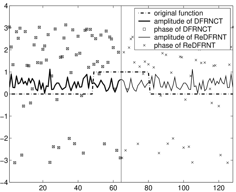
Figure 1: The results of DFRNCT and ReDFRNT of the 1-D signal $x_{1}$, with $\alpha=0.6$ and $M=1$. Because the function $x_{1}$ is even, so that the ReDFRNT are symmetrical and coincides with the DFRNCT.

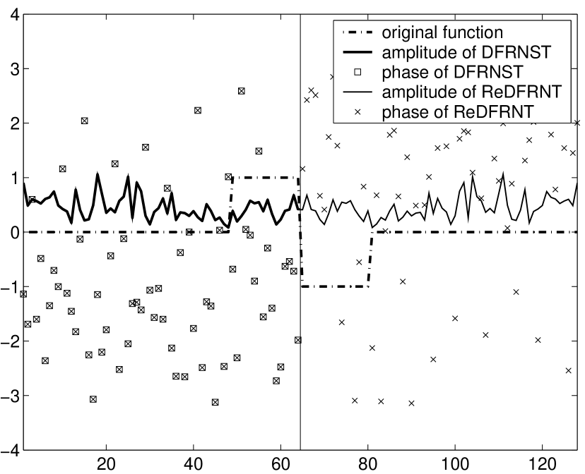
Figure 2: The results of DFRNST and ReDFRNT for the odd signal $x_{2}$ with $\alpha=0.6$ and $M=1$. The amplitude of ReDFRNT are symmetric and coincides with the result of DFRNST.

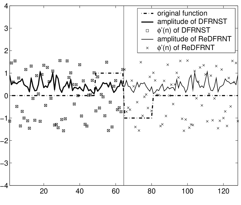
Figure 3: The same calculation results of DFRNST and ReDFRNT for the signal $x_{2}$ with special phase $\phi^{\prime}(n)$. Where we also take $\alpha=0.6$ and $M=1$. The special phase then is symmetric distributed for the ReDFRNT.

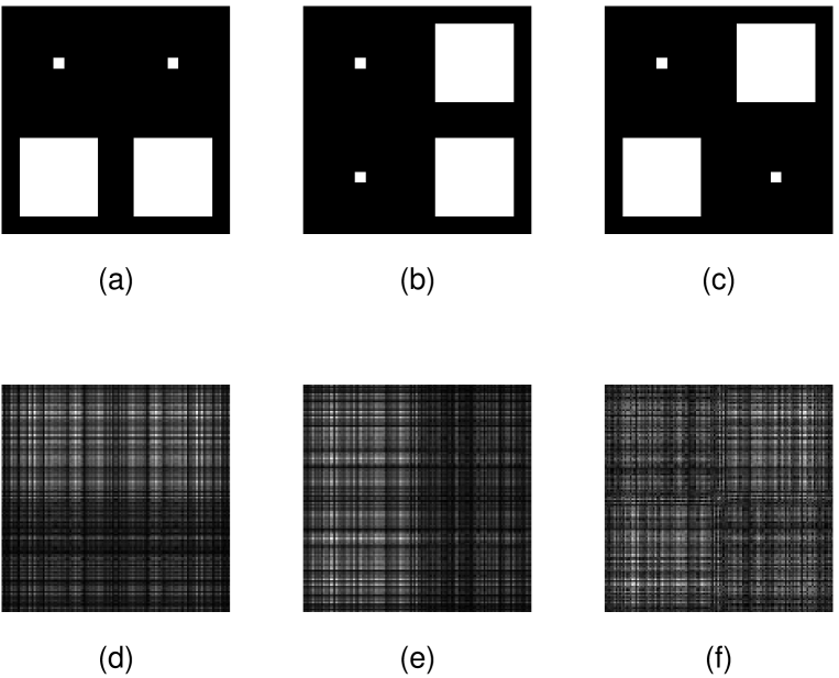
Figure 4: The results of ReDFRNT for 2-D functions: (a), (b) and (c) display three input images $I_{1}$, $I_{2}$ and $I_{3}$, respectively. From (d) to (f) are the corresponding ReDFRNT’s, with $\alpha=0.6$ and $M=1$, for images $I_{1}$, $I_{2}$ and $I_{3}$, respectively. From the results we can find that the ReDFRNT keep the symmetries in the input images.

References

- [1] Z. Liu, H. Zhao and S. Liu, A discrete fractional random transform, Opt. Comm. 255, (2005) 357.
- [2] H. M. Ozaktas, Z. Zalevsky, and M. A. Kutay, The fractional Fourier transform with applications in optics and signal processing, (New York: John Wiley & Sons), 2000.
- [3] S. C. Pei and M. H. Yeh, Improved discrete fractional Fourier transform, Opt. Lett. 22, (1997) 1407.
- [4] F. Bellifemine and R. Picco, Video signal coding with DCT and vector quantization, IEEE. Trans. Commun. 42, (1994) 200.
- [5] H. T. Chang and C. L. Tsan, Image watermarking by use of digital holography embedded in the discrete-cosine-transform domain, Appl. Opt. 44, (2005) 6211.
- [6] E. Y. Lam and J. W. Goodman, Discrete cosine transform domain restoration of defocused images, Appl. Opt. 37, (1998) 6213.
- [7] S. C. Pei and M. H. Yeh, The discrete fractional cosin and sine transform, IEEE Trans. Signal Processing, 49, (2001) 1198.
- [8] A. W. Lohmann, D. Mendlovic, Z. Zalevsky and R. G. Dorsch, Some important fractional transformations for signal processing, Opt. Comm. 125, (1996) 18.