A discrete fractional random transform

Abstract

We propose a discrete fractional random transform based on a generalization of the discrete fractional Fourier transform with an intrinsic randomness. Such discrete fractional random transform inheres excellent mathematical properties of the fractional Fourier transform along with some fantastic features of its own. As a primary application, the discrete fractional random transform has been used for image encryption and decryption.

1 Introduction

It is well known that the mathematical transforms from time (or space) to frequency domain or joint time-frequency domain, such as Fourier transform, Winger distribution function, wavelet transform and more recent fractional Fourier transform, etc. have long been powerful mathematical tools in physics and information processing. For instance, Fourier transform has been the basic tool for signal representation, analysis and processing, image processing and pattern recognition. In physics the Fourier transform describes well the Fraunhofer (far field) diffraction of light and thus has been the fundamental of information optics [1]. More recently, in the research of quantum information, Fourier transform algorithm has been adopted as an effective and fundamental algorithm in quantum computer [2]. Wavelet transform is a kind of windowed Fourier transform (Gabor transform), however with variable size of the windows [3]. Therefore wavelet transform has been an extremely powerful tool in signal representation in time-frequency joint domain with multi-resolution capability, and has been extensively used in image compression, segmentation, fusion and optical pattern recognitions.

The significance of mathematical transforms manifests itself further when the fractional Fourier transform was re-invented in 1980’s [4, 5] and became active from 1990’s after its physical interpretations were found in optics [6, 7, 8]. Actually at the beginning, Namias tried to solve Schrödinger equations in quantum mechanics using fractional Fourier transform as a tool with little notice in community. However, the fractional Fourier transform has found itself in real physical processes of light propagation in a graded index (GRIN) fiber, which is equivalent to a near field diffraction of light, Fresnel diffraction, with a quadratic factor. Thus the fractional Fourier transform can be easily realized in a bulk optical setup consisting of lenses. The fractional Fourier transform provides various of new mathematical operations which are useful in the field of optical information processing. And because fractional Fourier transform also is a kind of time-frequency joint representation of a signal [9], it has found extensive applications in signal and image processing [10].

The discrete forms of mathematical transforms have been extremely useful in applications, especially in signal processing and image manipulations. In fact, discrete transforms can approximate their continuous versions with high precision, meanwhile with high computation speed and lower complexities. Needless to say, Discrete Fourier transform (or FFT) and discrete wavelet transform have been widely used in different kinds of applications. Recently, discrete fractional Fourier transform (DFrFT) and the relevant discrete fractional cosine transform (DFrCT) have been proposed [11, 12]. We have used this fast algorithm of fractional Fourier transform in the numerical simulations of image encryption and optical security [13, 14].

As we have demonstrated that the extension of fractional Fourier transform have many different kinds of definitions according to how we fractionalize the Fourier transform [15], the DFrFT may also have different kinds of versions. In our researches of optical image encryption, we ask naturally the question, is there any possibility that the DFrFT be random? We have been motivated in searching such a random transform because then the image encryption process could be simplified by a single step of transform. Recently we found that, from the generalization of DFrFT, we can construct a discrete fractional random transform (DFRNT) with an inherent randomness. We demonstrate that such DFRNT has excellent mathematical properties as the fractional Fourier transforms have. And moreover it has some fantastic features of its own. We have also demonstrated that the DFRNT is a very efficient tool in digital image encryption and decryption with a very high speed of computation. The open questions left are concerning with the physical analogies of DFRNT and its further applications, which we are considering now.

We discuss the mathematical definition and properties of DFRNT and provide numerical simulation results of the DFRNT’s for one-dimensional and two-dimensional signals in the following sections in details.

2 Mathematics of the discrete fractional random transform

We begin our discussions from the definition of DFrFT proposed by Pei et al [11]. A one-dimensional DFrFT can be expressed as a matrix-vector multiplication

$$\mathbf{X}_{\alpha}(n)=\mathbf{F}^{\alpha}\mathbf{x}(n),$$ (1)

where $\mathbf{x}(n)$ is the input vector which has $N$ elements, $\mathbf{F}^{\alpha}$ is the kernel transform matrix and $\alpha$ is the fractional order. When $\alpha=1$, the DFrFT becomes the DFT as $\mathbf{X}(n)=\mathbf{F}\mathbf{x}(n)$, with matrix $\mathbf{F}$ indicating the kernel matrix of DFT.

The transform matrix is defined as follows. Firstly, because the fractional Fourier transform has the same eigenfunctions with the Fourier transform, we can calculate the eigenvectors $\{\mathbf{V}_{j}\}$ ($j=1,2,\dots,N$) of DFrFT with a real transform matrix $\mathbf{S}$ of discrete Fourier transform which is defined as follows [16]

$$\mathbf{S}=\left[\begin{array}[]{ccccccc}2&1&0&0&\dots&0&1\\ 1&2\cos\omega&1&0&\dots&0&0\\ 0&1&2\cos 2\omega&1&\dots&0&0\\ \vdots&\vdots&\vdots&\ddots&\vdots&\vdots&\vdots\\ 1&0&0&0&\dots&1&2\cos(N-1)\omega\end{array}\right],$$ (2)

where $\omega=2\pi/N$. The matrix $\mathbf{S}$ actually is not the kernel transform matrix $\mathbf{F}$ of the discrete Fourier transform (DFT). However, the matrix $\mathbf{S}$ commutes with matrix $\mathbf{F}$, i.e. $\mathbf{S}\mathbf{F}=\mathbf{F}\mathbf{S}$. Thus the eigenvectors of $\mathbf{S}$ are also the eigenvectors of $\mathbf{F}$, only they correspond to different eigenvalues. Because the matrix $\mathbf{S}$ is symmetrical, the eigenvectors {$\mathbf{V}_{j}$} are all real and orthonormal to each other. They form an orthonormal basis which is equivalent to the Hermite-Gaussian polynomials in the case of continuous Fourier transform and fractional Fourier transform. Therefore, from the matrix $\mathbf{S}$ we obtain the $N\times N$ eigenvector basis matrix $\mathbf{V}$, which is formed by the $N$ column eigenvectors $\{\mathbf{v}_{1},\mathbf{v}_{2},\dots,\mathbf{v}_{N}\}$ as $\mathbf{V}=\left[\mathbf{v}_{1}\;\mathbf{v}_{2}\;\dots\;\mathbf{v}_{N}\right]$. In the calculation of DFrFT, the DFT-shifted version of eigenvectors {$\mathbf{V}_{j}$} are taken.

Next step, we determine the eigenvalues of DFrFT. We know that the eigenvalues of the continuous fractional Fourier transform can be written as

$$\lambda_{k}=\exp(-i\alpha k\pi/2),\;k=0,1,2,\dots,\infty.$$ (3)

In DFrFT the eigenvalues are not changed, only we have a limited numbers of eigenvalues being taken into account, say $k=0,1,2,\dots,N$. Those eigenvalues again construct a matrix $\mathbf{D}_{\alpha}$ as follows

$$\mathbf{D}_{\alpha}=\left\{\begin{array}[]{llll}\mathrm{diag}\left(1,e^{-i\alpha\pi/2},\dots,e^{-i\alpha(N-1)\pi/2}\right)&\mbox{if $N$ is odd,}\\ \mathrm{diag}\left(1,e^{-i\alpha\pi/2},\dots,e^{-i\alpha(N-2)\pi/2},e^{-i\alpha N\pi/2}\right)&\mbox{if $N$ is even},\end{array}\right.$$ (4)

where $\mathbf{D}_{\alpha}$ is an $N\times N$ diagonal matrix. It must be noted that in the expression of $\mathbf{D}_{\alpha}$, there is a jump in the last eigenvalue for the $N$ is an even integer. Such assignments of eigenvalues of DFrFT are consistent with the DFT’s multiplicity rules [17].

So now we have already had the eigenvector basis $\mathbf{V}$ and the corresponding eigenvalues $\mathbf{D}_{\alpha}$. In the final step, we can express a kernel transform of DFrFT by the eigen-decomposition. The transform matrix of the DFrFT can then be defined as

$${\mathbf{F}}^{\alpha}=\mathbf{V}\mathbf{D}_{\alpha}\mathbf{V}^{T},$$ (5)

where $\mathbf{V}^{T}$ indicates the transpose of the matrix $\mathbf{V}$. Because the eigenvectors are orthonormal, we have $\mathbf{V}\mathbf{V}^{T}=\mathbf{I}$ and $\mathbf{I}$ is the identity matrix. And also $\mathbf{D}_{-\alpha}=\mathbf{D}_{\alpha}^{*}$. Those relations conform that the DFrFT have the same properties with the continuous FrFT.

The above procedure gives a formal way to construct the DFrFT. The matrix ${\mathbf{S}}$ is the most important figure in the both DFrFT and DFT, because from it the eigenvectors of DFT and DFrFT can be calculated. The matrix ${\mathbf{S}}$ is symmetrical and therefore its eigenvalues are all real and the eigenvectors are orthonormal. The transform kernel matrix of DFT and DFrFT can thus be constructed by eigen-decomposition with different eigenvalues.

How does a discrete fractional Fourier transform becomes random? The essence of the generalization from the DFrFT to DFRNT is to change the matrix $\mathbf{S}$ to a random matrix. The DFRNT can be defined by a symmetric random matrix $\mathbf{Q}$. The matrix $\mathbf{Q}$ is generated by an $N\times N$ real random matrix $\mathbf{P}$ with a relation of

$$\mathbf{Q}=(\mathbf{P}+\mathbf{P}^{T})/2,$$ (6)

where we have ${Q}_{lk}={Q}_{kl}$. Similar to the definition of DFrFT, we can also generate $N$ real orthogonal eigenvectors $\{\mathbf{v}^{\prime}_{R1},\mathbf{v}^{\prime}_{R2},\dots,\mathbf{v}^{\prime}_{RN}\}$ of matrix ${\mathbf{Q}}$. Those eigenvectors can be normalized by the Schmidt standard normalization procedure. Then we have $N$ orthonormal eigenvectors $\{\mathbf{v}_{R1},\mathbf{v}_{R2},\dots,\mathbf{v}_{RN}\}$. From those column vectors a matrix

$$\mathbf{V}_{R}=\left[\mathbf{v}_{R1}\;\mathbf{v}_{R2}\;\dots\;\mathbf{v}_{RN}\right]$$ (7)

can be achieved, where $\mathbf{V}_{R}\mathbf{V}_{R}^{T}=\mathbf{I}$. We do not need to DFT-shift the eigenvectors here, because these eigenvectors are generated from a symmetrical random matrix.

The coefficient matrix, that corresponds to the eigenvalues of DFRNT can be defined as

$$\mathbf{D}_{R\alpha} = \mathrm{diag}\left(1,\exp\left(-i\frac{2\pi\alpha}{M}\right),\exp\left(-i\frac{4\pi\alpha}{M}\right),\right.$$ (8)

$$\quad\quad\quad\quad\quad\quad\quad\quad\quad\left.\dots,\exp\left(-i\frac{2(N-1)\pi\alpha}{M}\right)\right),$$

which is used in the process of eigen-decomposition. One should notice that the eigenvalues of DFRNT are not necessarily relevant to those of DFrFT’s or DFT’s. However, we take a similar form so that the DFRNT may have similar mathematical properties. In Eq. (8) there is no jump for odd and even integer $N$. We introduce here an integer number $M$ in the coefficients. It indicates the periodicity of DFRNT with respect to the fractional order $\alpha$ whose significance will be shown bellow. The kernel transform matrix of DFRNT can thus be expressed as

$${\mathbf{R}}^{\alpha}=\mathbf{V}_{R}\mathbf{D}_{R\alpha}\mathbf{V}^{T}_{R}.$$ (9)

Therefore the DFRNT of a one-dimensional discrete signal is written as

$$\mathbf{X}_{R(\alpha)}(n)=\mathbf{R}^{\alpha}\mathbf{x}(n)$$ (10)

The expansion of DFRNT for two dimensional signal is straightforward as $\mathbf{X}_{R(\alpha)}=\mathbf{R}^{\alpha}\mathbf{x}\left(\mathbf{R}^{\alpha}\right)^{T}$.

The most important feature of DFRNT is that its transform kernel is random, which results from the randomness of matrix $\mathbf{Q}$, so that the result of transform is totally random. The eigenvectors of DFRNT depends upon the random matrix $\mathbf{Q}$ (or $\mathbf{P}$), therefore if we change the matrix $\mathbf{P}$, then the results of DFRNT’s is different. Furthermore, the DFRNT inheres most of the excellent properties of DFT (or DFrFT). It can be easily verified that the DFRNT has the following mathematical properties.

• Linearity, DFRNT is a linear transform, i.e. $\mathbf{R}^{\alpha}(a\mathbf{x}+b\mathbf{y})=a\mathbf{R}^{\alpha}\mathbf{x}+b\mathbf{R}^{\alpha}\mathbf{y}$, where $a$ and $b$ are constants.

• Unitarity, DFRNT is a unitary transform, i.e. $\mathbf{R}^{-\alpha}=\left(\mathbf{R}^{\alpha}\right)^{*}$ because $\mathbf{D}_{R(-\alpha)}=\mathbf{D}^{*}_{R\alpha}$. The inverse DFRNT exists and is defined as $\mathbf{R}^{-\alpha}$.

• Additivity, DFRNT obeys the additive role as the DFrFT (and FrFT) does for the fact that $\mathbf{R}^{\alpha}\mathbf{R}^{\beta}=\mathbf{R}^{\beta}\mathbf{R}^{\alpha}=\mathbf{R}^{\alpha+\beta}$.

• Multiplicity, DFRNT has a periodicity of $M$ in our definition, i.e. $\mathbf{R}^{\alpha+M}=\mathbf{R}^{\alpha}$, where we can change this periodicity with changing the integer $M$.

• Parseval, DFRNT satisfy the Parseval energy conservation theorem, i.e. $\sum_{k=0}^{N-1}\left|{X}_{\alpha(R)}(k)\right|^{2}=\sum_{m=0}^{N-1}\left|x(m)\right|^{2}$.

What we are interested most is randomness of DFRNT and the information retrieval capability because of its multiplicity. As the fractional order $\alpha=lM$, where $l$ is another integer, the DFRNT output signal $\mathbf{X}_{R(\alpha)}$ return to its original function $\mathbf{x}$. Otherwise, it will be totally random when the order $\alpha\neq lM$ even a small aberration occurs. While with the order $\alpha=lM/2$, i.e. at the half of its period, the output signal $\mathbf{X}_{R(\alpha)}$ is real. Such a fascinating feature can be rigorously proved in mathematics, because in this case $\mathbf{D}_{R\alpha}$ is real (and therefore the kernel transform matrix $\mathbf{R}^{\alpha}$ is real). It may also be intuitively seen if one recall that the Fourier transform has the property of $\mathcal{F}^{2}\{f(x)\}=f(-x)$. The only difference is that the amplitude of DFRNT, when $\alpha=lM/2$, is random but not $\left|\mathbf{x}(-n)\right|$.

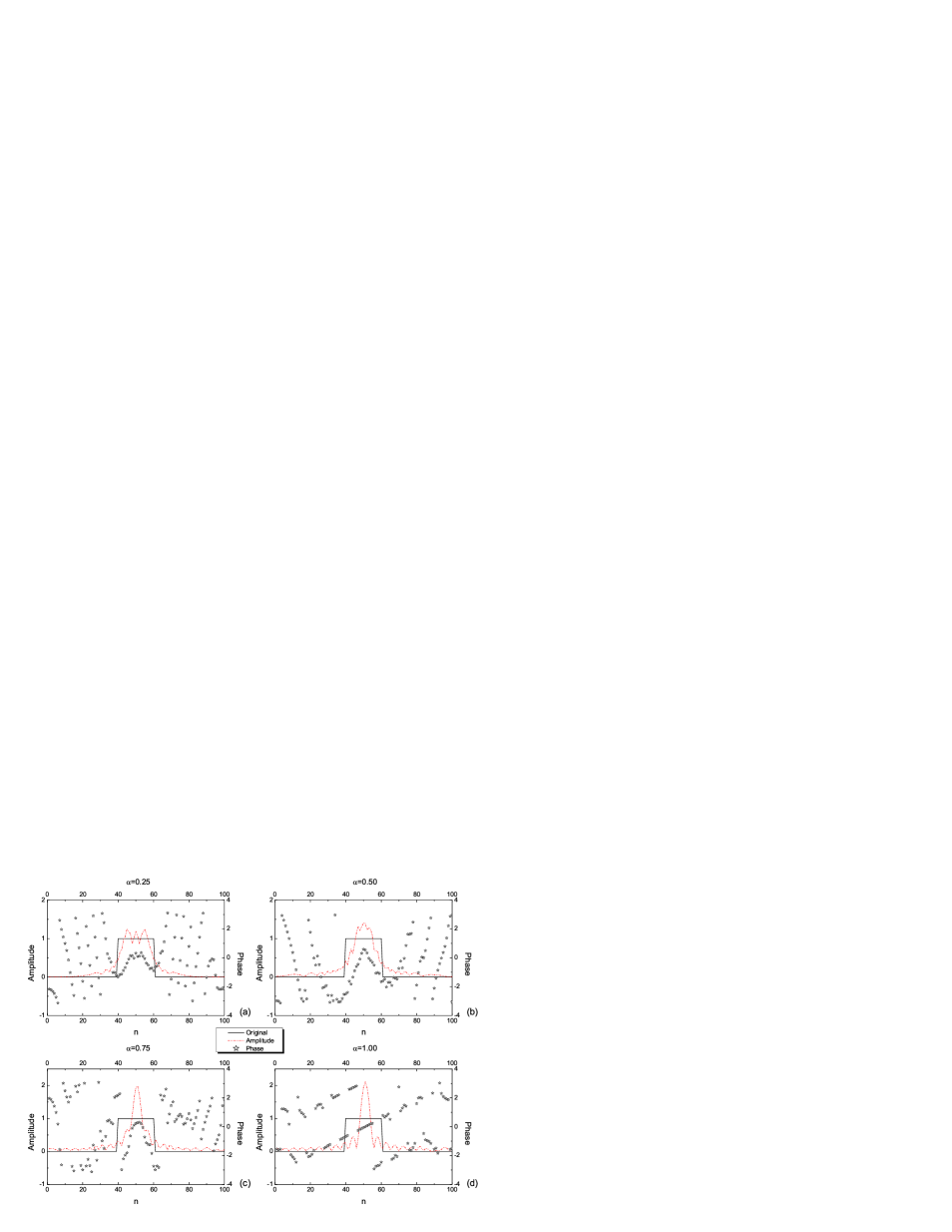
Figure 1: Numerical simulations of DFrFT of a one-dimensional rectangular window signal. The fractional orders are $\alpha=0.25$, $\alpha=0.50$, $\alpha=0.75$ and $\alpha=1.00$, respectively.

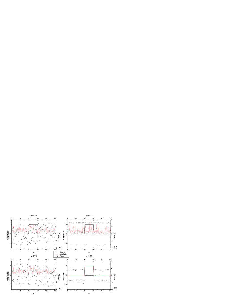
Figure 2: Numerical simulations of DFRNT of a one-dimensional rectangular window signal with normally distributed random numbers. The fractional orders are $\alpha=0.25$, $\alpha=0.50$, $\alpha=0.75$ and $\alpha=1.00$, respectively.

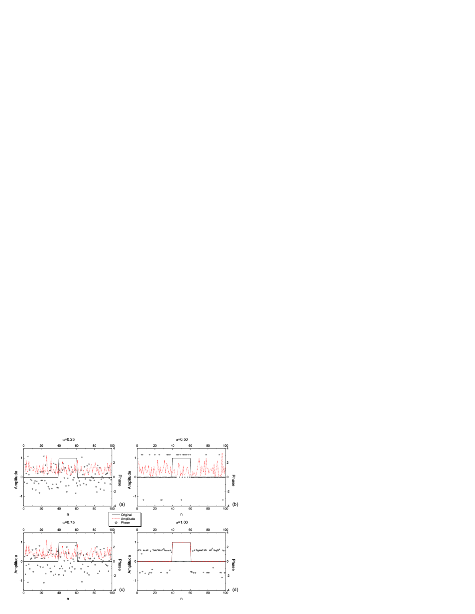
Figure 3: Numerical simulations of DFRNT of a one-dimensional rectangular window signal with uniformly distributed random numbers. The fractional orders are $\alpha=0.25$, $\alpha=0.50$, $\alpha=0.75$ and $\alpha=1.00$, respectively.

To illustrate the basic feature of DFRNT, and to make a comparison with DFrFT, we present here the simulation results for one-dimensional rectangular signal using DFrFT and DFRNT, in Fig. 1 to Fig. 3, respectively. The signal has a rectangular window with period of $[40,60]$. The total number of points is $N=100$. The numerical results of DFrFT is given in Fig. 1, with the fractional order $\alpha=0.25,\;0.50,\;0.75$ and $1.00$, respectively. We can see that the amplitudes of DFrFT’s gradually change from the original signal to its Fourier transform. However, the results will be different for the cases of DFRNT. We calculate DFRNT with two different formats of random numbers, one is normally distributed random number (illustrated in Fig. 2) and the other is uniform random number within $[0,1]$ (Fig. 3), as the matrix $\mathbf{P}$. Here we set the periodicity of DFRNT as $M=1$. From the results shown in Fig. 2 and Fig. 3, one can see that the amplitudes are all randomly distributed when the fractional order $\alpha\neq 1$. Whereas when $\alpha=1$, the output signal goes back to its original, i.e. the signal recovers.

Note that when $\alpha=0.50$, the phase values are $0$, $\pi$, or $-\pi$ whatever random matrix is used. That means we always get real transform results when the fractional order $\alpha$ is the half of the periodicity $M$. The amplitudes for $\alpha=0.25$ and $\alpha=0.75$ are the same, however their phases are conjugated. That is because $\mathbf{X}_{R(M-\alpha)}=\mathbf{X}_{R(-\alpha)}=\left(\mathbf{X}_{R(\alpha)}\right)^{*}$. When $\alpha=1$, the amplitudes of transformed signal totally retrieved, however, there exit about $\pm\pi/2$ phase fluctuations at the components of $x(k)=0$.

3 Image encryption and decryption: a primary application of DFRNT

The primary and perhaps the most important application of DFRNT is cryptography and information security. Because the DFRNT itself is random, the DFRNT of a two-dimensional signal can be directly used for image encryption with any fractional order $\alpha\neq lM$. The decryption process is simply an inverse DFRNT. The main encryption key is the matrix $\mathbf{Q}$. We have known that changing a random matrix $\mathbf{Q}$ indicates changing the present DFRNT to another DFRNT. The results are unrelated even they have the same fractional order $\alpha$. The DFRNT is quite sensitive to the random matrix and also to the fractional order, which have been demonstrated in our numerical simulations.

Numerical results of DFRNT’s of an image are given in Fig. 4 and Fig. 5 with normally and uniformly distributed random matrix respectively. The test image is the photo of Lenna with the size of $256\times 256$ pixels, shown in Fig. 4(a) and Fig. 5(a). The encryption process is simple, just an $\alpha$ order DFRNT with $\alpha\neq lM$. The encryption results are shown in Fig. 4(b), Fig. 4(c), Fig. 5(b) and Fig. 5(c), respectively, with $\alpha=0.50$ and $\alpha=0.80$. In our simulations we let $M=1$. The decryption is an inverse DFRNT with same random matrix $\mathbf{Q}$ and the fractional order $-\alpha$. However, if we perform the inverse DFRNT with another matrix $\mathbf{Q}$ which is different from the matrix we use in the encryption process, we fail to retrieve the image. The decryption results are shown in Fig. 4(d) and Fig. 5(d). And also it is worth to mention that the fractional order $\alpha$ can also be served as an extra decryption key. The inverse DFNRT’s with wrong fractional orders can not recover the image as shown in Fig. 4(e) and Fig. 5(e), with $\alpha=-0.502$ and $\alpha=-0.503$, respectively. As we have analyzed from the computation of mean square error (MSE), that the smallest security discrimination is about $|\Delta\alpha|_{min}\approx 0.02$ for normally distributed random matrix and $|\Delta\alpha|_{min}\approx 0.03$ for the case of uniformly distributed random matrix. When $|\Delta\alpha|>|\Delta\alpha|_{min}$, one can not visually recognize the image from the noisy background. The correct decryption results are shown in Fig. 4(f) and Fig. 5(f). The MSE for correct decryption process is in the order of $10^{-13}$ for both cases.

The image encryption with DFRNT using the fractional order $\alpha=lM/2$ is of great interest for real applications, because then the encrypted image has real values. It may be very useful for storing and transferring the secret data in a more convenient way, for example, by a photo plate.

The security strength of the DFRNT encryption can be estimated as $2^{N(N+1)/2}$ because the random matrix $\mathbf{Q}$ has $N(N+1)/2$ independent elements. As a matter of fact, if one try to search such a random matrix coded with uniformly distributed random numbers, the number of steps will be much larger than $2^{N(N+1)/2}$. Therefore, such an image encryption method is considerably secure in theory. This encryption algorithm can be easily implemented digitally.

Is there any applications of DFRNT in Physics? This question now is left for an open problem. Nevertheless, DFRNT has a powerful multiplicities with changing the formats of matrix $\mathbf{Q}$. The different matrix $\mathbf{Q}$ may results in different transform with different mathematical properties. Such a feature may be helpful in filter designs in signal and image processing. We can also establish an iterative mechanism that the matrix $\mathbf{Q}$ can be modified accordingly. This mechanism may be found applications in solving inverse problems in optics, such as the phase retrieval.

4 Conclusions

We have proposed a new kind of discrete transform, a discrete fractional random transform, based on a generalization of the discrete fractional Fourier transform. The intrinsic randomness of the discrete fractional random transform origins from a symmetrical random matrix, from which the eigenvectors of the transform are generated. The discrete fractional random transform inheres the excellent mathematical properties as the fractional Fourier transforms have. A new image encryption and decryption scheme is proposed that uses the discrete fractional random transform. Thus the processes of image encryption and decryption are very simple, only consisting of an operation of discrete fractional random transform and its inverse. Mathematical properties of the new discrete transform have been given in details with numerical demonstration.

List of figure captions

Figure 1. DFrFT of a one-dimensional rectangular window signal. The fractional orders are $\alpha=0.25$, $\alpha=0.50$, $\alpha=0.75$ and $\alpha=1.00$, respectively.

Figure 2. DFRNT of a one-dimensional rectangular window signal with normally distributed random numbers. The fractional orders are $\alpha=0.25$, $\alpha=0.50$, $\alpha=0.75$ and $\alpha=1.00$, respectively.

Figure 3. DFRNT of a one-dimensional rectangular window signal with uniformly distributed random numbers. The fractional orders are $\alpha=0.25$, $\alpha=0.50$, $\alpha=0.75$ and $\alpha=1.00$, respectively.

Figure 4. Numerical results of DFRNT with two-dimensional data using a normally distributed random matrix. DFRNT serves as an image encryption and decryption algorithm here. (a) The original image, (b) encrypted image with $\alpha=0.5$, (c) encrypted image with $\alpha=0.8$, (d) decryption result for image (b) with a different random matrix, (e) decryption result for image (b) with $\alpha=-0.502$, and (f) the correct decryption of the image.

Figure 5. Numerical results of DFRNT with two-dimensional data using a uniformly distributed random matrix. (a) The original image, (b) encrypted image with $\alpha=0.5$, (c) encrypted image with $\alpha=0.8$, (d) decryption result for image (b) with a different random matrix, (e) decryption result for image (b) with $\alpha=-0.503$, and (f) the correct decryption of the image.

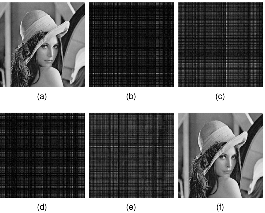
Figure 4: Numerical results of DFRNT with two-dimensional data using a normally distributed random matrix. DFRNT serves as an image encryption and decryption algorithm here. (a) The original image, (b) encrypted image with $\alpha=0.5$, (c) encrypted image with $\alpha=0.8$, (d) decryption result for image (b) with a different random matrix, (e) decryption result for image (b) with $\alpha=-0.502$, and (f) the correct decryption of the image.

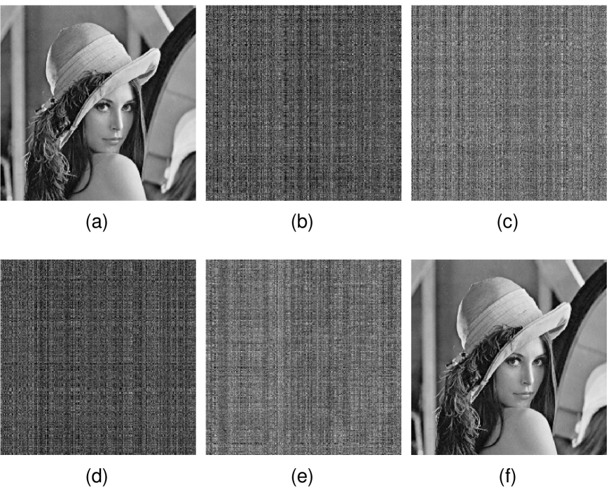
Figure 5: Numerical results of DFRNT with two-dimensional data using a uniformly distributed random matrix. DFRNT serves as an image encryption and decryption algorithm here. (a) The original image, (b) encrypted image with $\alpha=0.5$, (c) encrypted image with $\alpha=0.8$, (d) decryption result for image (b) with a different random matrix, (e) decryption result for image (b) with $\alpha=-0.503$, and (f) the correct decryption of the image.

References

- [1] J. W. Goodman, Introduction to Fourier Optics (New York: McGraw-Hill), 1968.
- [2] M. A. Nielsen and I. Chuang, Quantum computation and quantum information (Cambridge: Cambridge Uni. Press), 2000.
- [3] C. K. Chui, An intoduction to wavelets (Academic Press, Inc.), 1992.
- [4] V. Namias, The fractional Fourier order Fourier transform and its application to quantum mechanics, J. Inst. Maths Appl. 25, (1980) 241.
- [5] A. C. McBrdige and F. H. Kerr, On Namias’s fractional Fourier transforms, IMA J. Appl. Math. 39, (1987) 159.
- [6] D. Mendlovic and H. M. Ozaktas, Fractional Fourier transfroms and their optical implementation: I, J. Opt. Soc. Am. A10, (1993) 1875.
- [7] A. W. Lohmann, Image rotation, Wigner rotation, and the fractional order Fourier transform, J. Opt. Soc. Am. A10, (1993) 2181.
- [8] D. Mendlovic, H. M. Ozaktas and A. W. Lohmann, Graded-index fibers, Wigner-distibution functions, and the fractional Fourier transform, Appl. Opt. 33, (1994) 6188.
- [9] L. B. Almeida, The fractional Fourier transform and time-frequency representation, IEEE Trans. Sig. Proc. 42, (1994) 3084.
- [10] H. M. Ozaktas, Z. Zalevsky, and M. A. Kutay, The fractional Fourier transform with applications in optics and signal processing, (New York: John Wiley & Sons), 2000.
- [11] S. C. Pei and M. H. Yeh, Improved discrete fractional Fourier transform, Opt. Lett. 22, (1997) 1407.
- [12] S. C. Pei and M. H. Yeh, The discrete fractional cosine and sine transforms, IEEE Trans. Sig. Proc. 49, (2001) 1198.
- [13] S. Liu, L. Yu, and B. Zhu, Optical image encryption by cascaded fractional Fourier transforms with random phase filtering, Opt. Commun. 187, (2001) 57.
- [14] S. Liu , Q. Mi, and B. Zhu. Optical image encryption with multi-stage and multi-channel fractional Fourier domain filtering, Opt. Lett. 26, (2001) 1242.
- [15] S. Liu, J. Jiang, Y. Zhang and J. Zhang, Generalized fractional Fourier transforms, J. Phys. A: Math & Gen. 30, (1997) 973.
- [16] B. W. Dickinson and K. Steiglitz, Eigenvectors and functions of the discrete Fourier transform IEEE Trans. Acoust. Speech. & Sig. Proc. ASSP-30, (1982) 25.
- [17] J. H. McCellan and T. W. Parks, Eigenvalue and eigenvector decomposition of the discrete Fourier transform, IEEE Trans. Audio Electroacoustics 20, (1972) 66.