SLE Local Martingales, Reversibility and Duality

Abstract

We study SLE reversibility and duality using the Virasoro structure of the space of local martingales. For both problems we formulate a setup where the questions boil down to comparing two processes at a stopping time. We state algebraic results showing that local martingales for the processes have enough in common. When one has in addition integrability, the method gives reversibility and duality for any polynomial expected value.

Kalle Kyt l and Antti Kemppainen

Department of Mathematics and Statistics
P.O.Box 68, FIN-00014 University of Helsinki, Finland.
email: kalle.kytola@helsinki.fi and antti.h.kemppainen@helsinki.fi

1 Introduction

Schramm-Loewner Evolutions (SLEs) are conformally invariant random curves in two dimensions and their most important properties are determined by one parameter $\kappa\geq 0$. SLEs provide insight and a powerful method to global geometric questions in conformally invariant 2-d statistical physics at criticality. Therefore they complement the conformal field theory methods. SLEs have been successful in obtaining rigorous results about continuum limits of critical percolation ($\kappa=6$) [1], loop erased random walk ($\kappa=2$), uniform spanning tree ($\kappa=8$) [2] and massless free field level lines ($\kappa=4$) [3] but one expects results for many other models as well. In addition to the question of applying SLE to specific models of statistical physics, one can ask questions about SLEs themselves. In the seminal article [4] many fundamental properties of SLEs were worked out. Among the most important open problems, that paper states conjectures of reversibility and duality.

A chordal SLE is a random curve connecting two points on the boundary. The clever method of Loewner makes the whole SLE industry possible, but at the same time the description is made asymmetric by declaring one a starting point and the other an end point. SLE is said to be reversible if the curve is the same when we change the roles of the two points. Almost without an exception the question of reversibility is immediate in models of statistical mechanics. In fact, reversibility is known for SLE for some values of the parameter $\kappa$ because of work that shows that SLE_κ is the continuum limit of some model. Hidden in our approach to reversibility are conformal field theory concepts that again bring the starting and end points to the same status: the operators at the two points have the same conformal weight $h(\kappa)$ and both have a vanishing descendant at level two. The vanishing descendants manifest themselves in our formalism as null field equations for a partition function $Z$.

If the reversibility property is obvious in models of statistical mechanics, one might think that SLE reversibility is not a particularly interesting question from physics point of view. But conversely, failure of SLE reversibility would mean losing hope of describing the continuum limit of physical models by SLEs.

Duality is a conjectural property of SLEs that is likely to give a new kind of geometric insight to two dimensional critical phenomena. The conjecture relates SLEs with two parameter values where the SLEs have totally different behavior. The statement of the conjecture was originally vague: for $\kappa<4$ the boundary of SLE_16/κ hull looks locally like the SLE_κ trace. This conjecture is supported by considerations of fractal dimensions, a few examples of models of statistical mechanics and yet another conformal field theory concept: the central charge $c$, which takes the same value for SLE_κ and SLE_16/κ, i.e. $c(\kappa)=c(16/\kappa)$. We don’t claim to provide a satisfactory explanation of the origin of duality, but working on the precise form of the conjecture by Dubédat [5, 6], we show an algebraic reason for a class of expected values to possess the duality property.

As opposed to reversibility, duality seems directly physically relevant. As an example, it is believed that in critical $q$ state Potts model for $q\leq 4$, spin cluster boundaries in the continuum limit should be SLE_κ(q) curves with $\kappa(q)=4\cos^{-1}(-\sqrt{q}/2)/\pi\leq 4$. Potts models admit also a Fortuin-Kasteleyn random cluster model description. The boundaries of these FK clusters should look like SLE_16/κ(q) for $q\in[0,4]$. Duality would relate these different physical objects in a nontrivial geometric way. Besides the Potts model, there might be other cases of similar type. For $O(n)$ model in its graphical expansion, spin-spin correlation functions involve lattice curves connecting the points of insertion of spins. At critical point and as lattice mesh goes to zero, these curves for $n\in[0,2]$ are conjectured to become SLE_κ(n), where $\kappa(n)=4\pi/\cos^{-1}(-n/2)\in[8/3,4]$. Since $O(n)$ model allows rewritings of the same kind as the Potts model [7], it would be interesting to know whether these involve objects whose scaling limit is SLE_16/κ(n) and whether SLE duality gives insights regarding this. The relation to SLE of many statistical mechanics models is reviewed in [11].

This letter introduces a setup for the questions of reversibility and duality using the Virasoro module structure of the space of local martingales explained in [8]. We state algebraic results supporting both conjectures. The aim is to compute the behavior of martingales as distances between certain points tend to zero. Underlying the computations must be the CFT concepts of fusion and operator product expansions. In forthcoming articles [17] we will provide more careful proofs, discuss the mathematics in more detail and apply a wider set of methods.

2 Schramm-Loewner Evolutions

The definition of SLEs appropriate for this note is most conveniently given in the half plane $\mathbb{H}=\{z\in\mathbb{C}:\Im\textrm{m }z>0\}$ and allowing the level of generality of [9]. For comprehensive introduction to SLE we recommend e.g. [10, 11, 12]. The SLE map $g_{t}$ is a solution of the Loewner equation

$$\frac{\mathrm{d}}{\mathrm{d}t}g_{t}(z)=\frac{2}{g_{t}(z)-X_{t}}$$

with initial condition $g_{0}(z)=z$. The map $g_{t}$ is conformal from $\mathbb{H}\setminus K_{t}$ to $\mathbb{H}$, where $K_{t}$ is called the SLE hull at time $t$. The Loewner equation involves a real valued process $t\mapsto X_{t}\in\mathbb{R}=\partial\mathbb{H}$, the driving process, and we also allow dependency on a number of real points $Y^{K}_{t}=g_{t}(Y^{K}_{0})$, $K=1,\ldots,M$, that follow passively the Loewner flow. We assume the driving process to solve the Itô stochastic differential equation

$$\mathrm{d}X_{t}=\sqrt{\kappa}\;\mathrm{d}B_{t}+\kappa(\frac{\partial}{\partial x}\log Z)(X_{t};Y^{1}_{t},\ldots,Y^{M}_{t})\;\mathrm{d}t\textrm{ ,}$$

where $Z(x;y_{1},\ldots,y_{M})$ is the partition function (auxiliary function), which is annihilated by the operator

$$\mathcal{D}^{(x)}=\frac{\kappa}{2}\frac{\partial^{2}}{\partial x^{2}}+\sum_{K=1}^{M}\big{(}\frac{2}{y_{K}-x}\frac{\partial}{\partial y_{K}}-\frac{2\delta_{y_{K}}}{(y_{K}-x)^{2}}\big{)}\textrm{ .}$$

The numbers $\delta_{y_{K}}$ are called the conformal weights at points $Y^{K}_{0}$. The equation $\mathcal{D}^{(x)}Z=0$ is called a null field equation and it is interpreted in conformal field theory as a vanishing descendant of the operator at the position $x$ of the driving process.

When $Z$ is of a product form, the process is SLE${}_{\kappa}(\rho_{1},\ldots,\rho_{M})$, introduced in [5] in the course of studying SLE duality. The concrete expression

$$Z(x;y_{1},\ldots,y_{M})=\Big{(}\prod_{K=1}^{M}(y_{K}-x)^{\rho_{K}/\kappa}\Big{)}\Big{(}\prod_{1\leq J<K\leq M}(y_{J}-y_{K})^{\rho_{J}\rho_{K}/2\kappa}\Big{)}$$

was given in [9] and the conformal weights are $\delta_{y_{K}}=\rho_{K}(\rho_{K}+4-\kappa)/4\kappa$.

The SLE trace $\gamma$ is the (random) curve in $\overline{\mathbb{H}}$ defined by $\gamma(t)=\lim_{\varepsilon\downarrow 0}g^{-1}_{t}(X_{t}+i\varepsilon)$. Existence of the limit and continuity of $t\mapsto\gamma(t)$ were proved in [4]. The hull is generated by the trace in the sense that $\mathbb{H}\setminus K_{t}$ is the unbounded component of $\mathbb{H}\setminus\gamma[0,t]$. There is a transition in the qualitative properties of the trace: for $\kappa\leq 4$ the trace $\gamma$ is a simple path and $K_{t}=\gamma[0,t]$ whereas for $\kappa>4$ we have $\gamma[0,t]\subsetneq K_{t}$ and the trace touches itself and $\partial\mathbb{H}=\mathbb{R}$.

3 The Virasoro module $\mathcal{M}$ of local martingales

In [8] one of us showed how the local martingales of SLE form a Virasoro module. We briefly explain the result.

Denote the formal power series in $z$ whose coefficients are the independent variables $f_{m}$, $m\leq-2$, by

$$f(z)=z+\sum_{m\leq-2}f_{m}z^{1+m}\textrm{ .}$$

Notations such as $f^{\prime}(z)$ and $Sf(z)=\frac{f^{\prime\prime\prime}(z)}{f^{\prime}(z)}-\frac{3}{2}\frac{f^{\prime\prime}(z)^{2}}{f^{\prime}(z)^{2}}$ and rational functions of $f$ are understood as formal power series at infinity, always containing only finitely many positive powers of the argument. Residue of a formal power series in $z$ is the coefficient of $z^{-1}$. Given $\delta_{(\cdot)}$, $Z$ as in Section 2 and $c\in\mathbb{C}$, we can define the operators

$$\mathcal{L}_{n}\,=\, \mathrm{Res}_{r}\;r^{1-n}\Big{\{}\frac{c}{12}Sf(r)+\frac{\delta_{x}\,f^{\prime}(r)^{2}}{(f(r)-x)^{2}}+\frac{\partial_{x}Z}{Z}\;\frac{f^{\prime}(r)^{2}}{f(r)-x}$$

$$\qquad+\sum_{K}\big{(}\frac{\delta_{y_{K}}\,f^{\prime}(r)^{2}}{(f(r)-y_{K})^{2}}+\frac{\partial_{y_{K}}Z}{Z}\;\frac{f^{\prime}(r)^{2}}{f(r)-y_{K}}\big{)}$$

$$\qquad+\frac{f^{\prime}(r)^{2}}{f(r)-x}\;\frac{\partial}{\partial x}+\sum_{K}\frac{f^{\prime}(r)^{2}}{f(r)-y_{K}}\;\frac{\partial}{\partial y_{K}}$$

$$\qquad-\sum_{l\leq-2}\mathrm{Res}_{z}\;z^{-2-l}\frac{f^{\prime}(r)^{2}}{f(z)-f(r)}\;\frac{\partial}{\partial f_{l}}\Big{\}}$$

on a suitable function space $\mathcal{F}\big{(}x,(y_{K})_{1\leq K\leq M},(f_{l})_{l\leq-2}\big{)}$. A mere change of notation from [8] shows that the operators $\mathcal{L}_{n}$ satisfy the commutation relations of the Virasoro algebra $\mathfrak{vir}$ (for Virasoro algebra and its representations see e.g. [13] and [14]). For both geometric and algebraic reasons we assign degree $1$ to the variables $x,y_{1},\ldots,y_{M}$ and degree $m$ to $f_{-m}$. The degree of a monomial is the sum of degrees of its variables, counting multiplicities.

Local martingales are functions $\varphi$ such that the Itô derivative of $\varphi(X_{t},\ldots,Y^{M}_{t};g_{-2}(t),\ldots)$ has no drift term, i.e.

$$\mathrm{d}\varphi(X_{t};Y^{1}_{t},\ldots,Y^{M}_{t};g_{-2}(t),g_{-3}(t),\ldots)=0\;\mathrm{d}t+(\cdots)\;\mathrm{d}B_{t}\textrm{ .}$$

The operators $\mathcal{L}_{n}$ were shown to preserve the space of local martingales for the specific values $\delta_{x}=h(\kappa)=\frac{6-\kappa}{2\kappa}$ and $c=c(\kappa)=\frac{(3-8\kappa)(6-\kappa)}{2\kappa}$. Starting from the constant function $1$ and applying in all possible ways the operators $\mathcal{L}_{n}$ one generates the $\mathfrak{vir}$ module

$$\mathcal{M}=\mathcal{U}(\mathfrak{vir})\cdot 1$$

that consists of local martingales. In fact, as shown in [8], if $Z$ is translation invariant and homogeneous, $\mathcal{M}$ is a highest weight module for $\mathfrak{vir}$ with the constant function $1$ as its highest weight vector.

For $\kappa\notin\mathbb{Q}$, any Verma module for $\mathfrak{vir}$ with central charge $c(\kappa)$ is either irreducible or contains a maximal submodule generated by a single singular vector [14]. We refer to this case as generic $\kappa$.

4 Setup for Reversibility

The chordal SLE from $0$ to $\infty$ in $\mathbb{H}$ can be viewed as an SLE with no extra points $Y$ and constant partition function $Z(x)=1$. The reversibility conjecture states that the trace $\gamma$ has the same law as the image of $\gamma$ under the inversion $z\mapsto-1/z$ of $\mathbb{H}$. The latter is the trace of an SLE from $\infty$ to $0$ in $\mathbb{H}$.

For the question of reversibility we find it more convenient to compare the chordal SLE from $X_{0}\in\mathbb{R}$ to $Y_{0}\in\mathbb{R}$ and from $Y_{0}$ to $X_{0}$, see Figure 1. This is obtained by a Möbius coordinate change from the usual chordal SLE, see e.g. [15, 16]. This variant is SLE${}_{\kappa}(\rho)$, $\rho=\kappa-6$, and the appropriate partition function is $Z(x,y)=(y-x)^{\frac{\kappa-6}{\kappa}}$. The conformal weight at the driving process and at the endpoint is the same, $\delta_{x}=\delta_{y}=h(\kappa)=\frac{6-\kappa}{2\kappa}$. The Loewner equation for an SLE from $X_{0}$ to $Y_{0}$ is $\dot{g}^{+}_{t}=2/(g^{+}_{t}-X^{+}_{t})$, where the driving process is $\mathrm{d}X^{+}_{t}=\sqrt{\kappa}\;\mathrm{d}B_{t}+\kappa(\partial_{x}\log Z)\;\mathrm{d}t$ and the other point $Y^{+}_{t}=g^{+}_{t}(Y_{0})$ is passive. The process is defined up to the stopping time $\tau^{+}$ at which $\lim_{t\uparrow\tau^{+}}|Y^{+}_{t}-X^{+}_{t}|=0$. At the end, $g^{+}_{\tau^{+}}$ maps the “outside” $\mathbb{H}\setminus K^{+}_{\tau^{+}}$ of the SLE trace conformally onto $\mathbb{H}$.

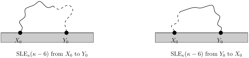
Figure 1: The two processes for reversibility.

To get a physical picture, consider for example the Ising model (believed to correspond to $\kappa=3$). Imposing boundary conditions $\uparrow$ on $[X_{0},Y_{0}]$ and $\downarrow$ on the rest of the real axis, the hull $K^{+}_{\tau^{+}}$ would be a component disconnected from $\infty$ by the curve $\gamma$ from $X_{0}$ to $Y_{0}$ that follows spin cluster boundaries.

The reverse case, an SLE from $Y_{0}$ to $X_{0}$ is obtained with the same partition function — one should observe that $Z(x,y)=(y-x)^{\frac{\kappa-6}{\kappa}}$ is annihilated not only by $\mathcal{D}^{(x)}$ but also by

$$\mathcal{D}^{(y)}=\frac{\kappa}{2}\frac{\partial^{2}}{\partial y^{2}}+\frac{2}{x-y}\frac{\partial}{\partial x}-\frac{2\delta_{x}}{(x-y)^{2}}\textrm{ .}$$

The Loewner equation $\dot{g}^{-}_{t}=2/(g^{-}_{t}-Y^{-}_{t})$ has $Y^{-}_{t}$ as its driving process, $\mathrm{d}Y^{-}_{t}=\sqrt{\kappa}\;\mathrm{d}B_{t}+\kappa(\partial_{y}\log Z)\;\mathrm{d}t$, and as a passive point $X^{-}_{t}=g^{-}_{t}(X_{0})$. At stopping time $\tau^{-}$ when $Y^{-}$ and $X^{-}$ collide, $K^{-}_{\tau^{-}}$ and $g^{-}_{\tau^{-}}$ are expected to have the same law as $K^{+}_{\tau^{+}}$ and $g^{+}_{\tau^{+}}$ in the non-reversed case — this is precisely the content of the reversibility conjecture for $\kappa\leq 4$.

Before we start the general consideration, let’s give a concrete illustration of the technique. The coefficient $g_{-2}(t)$, called the half-plane capacity, measures the size of $K_{t}$: for example if $g_{-2}(t)\leq R^{2}$ then the radius of $K_{t}$ is not more than $R$. The function $\mathcal{L}_{-2}\cdot 1\in\mathcal{M}$ is easily computed to be $-f_{-2}\,c(\kappa)/2+(y-x)^{2}\,h(\kappa)$. Therefore $-\frac{c(\kappa)}{2}g^{+}_{-2}(t)+h(\kappa)\,(Y^{+}_{t}-X^{+}_{t})^{2}$ is a local martingale. Supposing that it is in fact a closable martingale (if $\mathbb{E}[g_{-2}^{+}(\tau^{+})]<\infty$, it is), we can compute the average of $g_{-2}^{+}(\tau^{+})$ because expected values of martingales are constant in time

$$\mathbb{E}[-\frac{c(\kappa)}{2}g_{-2}^{+}(\tau^{+})]\;=\; \mathbb{E}\big{[}\big{(}\mathcal{L}_{-2}\cdot 1\big{)}(X^{+}_{\tau^{+}},Y^{+}_{\tau^{+}};g_{-2}^{+}(\tau^{+}))\big{]}$$

$$\;=\; \mathbb{E}\big{[}\big{(}\mathcal{L}_{-2}\cdot 1\big{)}(X^{+}_{0},Y^{+}_{0};g_{-2}^{+}(0))\big{]}=\mathbb{E}[h(\kappa)(Y_{0}-X_{0})^{2}]\textrm{ .}$$

Here we read that the average size of $K^{+}_{\tau^{+}}$ in terms of capacity is $\frac{2}{8-3\kappa}(Y_{0}-X_{0})^{2}$, which makes sense for $\kappa<8/3$. The same can be done with $g_{-2}^{-}(\tau^{-})$ and one finds that at least the average capacity is same for the reversed case (this is not new, though). Our strategy is to pick more complicated local martingales from $\mathcal{M}$ to determine more general expected values.

Since $Z(x,y)$ is the same for the SLE from $X_{0}$ to $Y_{0}$ and the reversed SLE, the representation $\mathcal{M}$ is obviously the same for both cases. Both cases are SLEs in the sense of Section 2, one with driving process $x$ and null field equation $\mathcal{D}^{(x)}Z=0$, the other with driving process $y$ and null field equation $\mathcal{D}^{(y)}Z=0$. Now as a consequence of $c=c(\kappa)$ and $\delta_{x}=\delta_{y}=h(\kappa)$, for any $\varphi\in\mathcal{M}=\mathcal{U}(\mathfrak{vir})\cdot 1$ the process

$$\varphi(X^{\pm}_{t},Y^{\pm}_{t};g^{\pm}_{-2}(t),g^{\pm}_{-3}(t),\ldots)$$

is a local martingale for both “$+$” and “$-$”.

The elements $\mathcal{L}_{-n_{1}}\cdots\mathcal{L}_{-n_{k}}\cdot 1$ that span the representation $\mathcal{M}$ are homogeneous polynomials of degree $\sum_{j}n_{j}$ in $x,y,f_{-2},f_{-3},\ldots$ (recall that $f_{-m}$ was assigned a degree $m$). This is because $\mathcal{L}_{-n}$ are differential operators containing only polynomial multiplications and they raise the degree by $n$. So $\mathcal{M}$ is a subspace of the space of polynomials, $\mathcal{M}\subset\mathbb{C}[x,y,f_{-2},\ldots]$. One also directly checks that $\mathcal{L}_{0}\cdot 1=0$ so $\mathcal{M}$ is a highest weight representation of highest weight $0$. By induction, keeping track of contributions of different parts of the operator $\mathcal{L}_{n}$ one establishes the important fact that $\mathcal{L}_{-n_{1}}\cdots\mathcal{L}_{-n_{k}}\cdot 1$ can be written as

$$P_{n_{1},\ldots,n_{k}}(f_{-2},\ldots)+(y-x)R_{n_{1},\ldots,n_{k}}(x,y;f_{-2},\ldots)\textrm{ ,}$$

where $P$ and $R$ are polynomials. This captures the behavior of the local martingale as $X$ and $Y$ processes come together, namely only the $P$ part remains in the limit $|x-y|\rightarrow 0$. The $P$ themselves form a highest weight module $\mathcal{P}=\mathrm{span}\;\{P_{n_{1},\ldots,n_{k}}\}\subset\mathbb{C}[f_{-2},f_{-3},\ldots]$ with highest weight vector $1$ in the obvious way.

The usefulness of the above is the consequence that local martingales for both processes have the same initial and final values and dependence of the quite different stochastic processes $X^{\pm}_{t}$, $Y^{\pm}_{t}$ disappears in the end. More precisely, choose $\varphi\in\mathcal{M}$ and denote its decomposition by $\varphi=P+(y-x)R$. Then $\varphi$ is a local martingale for both the SLE from $X_{0}$ to $Y_{0}$ and for the SLE from $Y_{0}$ to $X_{0}$. Moreover, its initial value at $t=0$ is the same for the two processes

$$\varphi(X^{\pm}_{0},Y^{\pm}_{0};g^{\pm}_{-2}(0),\ldots)=P(0,0,\ldots)+(Y_{0}-X_{0})R(X_{0},Y_{0};0,0,\ldots)$$

and the final value at $t=\tau^{\pm}$ is the same function of the coefficients of $g^{\pm}_{\tau^{\pm}}$

$$\varphi(X^{\pm}_{\tau^{\pm}},Y^{\pm}_{\tau^{\pm}};g^{\pm}_{-2}(\tau^{\pm}),\ldots)=P(g^{\pm}_{-2}(\tau^{\pm}),g^{\pm}_{-3}(\tau^{\pm}),\ldots)\textrm{ .}$$

In the case of reversibility, we can actually make an estimate of $L^{1}(\mathbb{P})$ norm to show that for $\kappa<8/(1+\sum_{j}n_{j})$, $\mathcal{L}_{-n_{1}}\cdots\mathcal{L}_{-n_{k}}\cdot 1$ is a closable martingale up to the stopping time $\tau^{\pm}$. Using this and the above observations of $\phi\in\mathcal{M}$, we establish reversibility of expected values of $P$.

Theorem 1

Let $\varphi=P+(y-x)R\in\mathcal{M}$ as above. For $\kappa$ small enough, the random variables $P(g^{\pm}_{-2}(\tau^{\pm}),g^{\pm}_{-3}(\tau^{\pm}),\ldots)$ are integrable, $\varphi(X^{\pm}_{t},Y^{\pm}_{t};g^{\pm}_{-2}(t),\ldots)$ are closable martingales up to the stopping times $\tau^{\pm}$ and consequently

$$\mathbb{E}[P(g^{\pm}_{-2}(\tau^{\pm}),g^{\pm}_{-3}(\tau^{\pm}),\ldots)]=P(0,0,\ldots)+(Y_{0}-X_{0})\;R(X_{0},Y_{0};0,0,\ldots)\textrm{ .}$$

Having discussed reversibility we now turn to the other question, duality. The strategy will be similar, even if the cumbersome details make it less transparent.

5 Setup for Duality

Recall that for $\kappa\leq 4$ the SLE_κ trace is a simple curve. For $\kappa>4$ the trace generates a strictly larger hull $K_{t}$, and the boundary of the hull, $\partial K_{t}$, can be parametrized as a continuous curve. The duality conjecture states roughly that for $0<\kappa<4$ and $\kappa^{*}=16/\kappa$, the boundary of the hull of SLE${}_{\kappa^{*}}$ looks like the trace of SLE_κ. The conjecture was formulated more precisely by Dubédat in [5, 6]. The processes we consider below are obtained by a coordinate change from Dubédat’s formulation. The general idea is again to compare the two processes at their stopping times. The driving process and other points will come together and we decompose local martingales accordingly. The decompositions show that we have continuous local martingales with same initial and final values, exactly as in the case of reversibility. The setup is explained in the paragraphs below and illustrated in Figure 2.

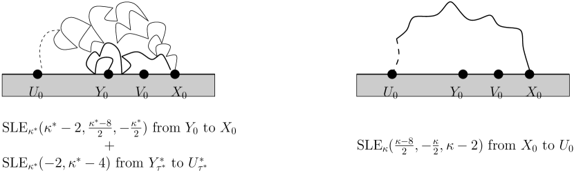
Figure 2: The two processes for duality.

Fix $\kappa<4$ and points $U_{0}<Y_{0}<V_{0}<X_{0}$. Instead of an ordinary SLE_κ we start from $X_{0}$ an SLE${}_{\kappa}(\rho_{u},\rho_{y},\rho_{v})$, where $\rho_{u}=\frac{\kappa-8}{2}$, $\rho_{y}=-\frac{\kappa}{2}$ and $\rho_{v}=\kappa-2$. The partition function is

$$Z\;=\; (y-u)^{\Delta_{y,u}}(v-u)^{\Delta_{v,u}}(x-u)^{\Delta_{x,u}}(v-y)^{\Delta_{v,y}}(x-y)^{\Delta_{x,y}}(x-v)^{\Delta_{x,v}}\textrm{ ,}$$

with the values of $\Delta_{(\cdot,\cdot)}$ and conformal weights $\delta_{(\cdot)}$ listed in Table 1 (a). The partition function satisfies $\mathcal{D}^{(x)}Z=0$ and the value of $\delta_{x}$ is $\delta_{x}=h(\kappa)$ again. The Loewner flow is $\dot{g}_{t}=2/(g_{t}-X_{t})$ and $\mathrm{d}X_{t}=\sqrt{\kappa}\;\mathrm{d}B_{t}+\kappa(\partial_{x}\log Z)\;\mathrm{d}t$ whereas the rest of the points are passive, $U_{t}=g_{t}(U_{0})$, $Y_{t}=g_{t}(Y_{0})$, $V_{t}=g_{t}(V_{0})$. Such an SLE will start from $X_{0}$ and end at $U_{0}$ at time $\tau$ at which $U_{\tau}=Y_{\tau}=V_{\tau}=X_{\tau}$.

	$u$	$y$	$v$	$x$
$u$		$\frac{8-\kappa}{8}$	$\frac{(\kappa-2)(\kappa-8)}{4\kappa}$	$\frac{\kappa-8}{2\kappa}$
$y$			$\frac{2-\kappa}{4}$	$-\frac{1}{2}$	$\Delta_{(\cdot,\cdot)}$
$v$				$\frac{\kappa-2}{\kappa}$
	$\frac{8-\kappa}{16}$	$\frac{3\kappa-8}{16}$	$\frac{\kappa-2}{2\kappa}$	$\frac{6-\kappa}{2\kappa}$	$\delta_{(\cdot)}$

	$\tilde{u}^{*}$	$\tilde{y}^{*}$	$\tilde{w}^{*}$
$\tilde{u}^{*}$		$-\frac{2}{\kappa^{*}}$	$\frac{4-\kappa^{*}}{\kappa^{*}}$
$\tilde{y}^{*}$			$\frac{\kappa^{*}-4}{\kappa^{*}}$	$\Delta_{(\cdot,\cdot)}$
	$\frac{\kappa^{*}-2}{2\kappa^{*}}$	$\frac{6-\kappa^{*}}{2\kappa^{*}}$	$0$	$\delta_{(\cdot)}$

Table 1: Values of $\Delta$ and $\delta$ in the duality setup

As in Section 4, a concrete illustration of the general technique is determining the average capacity of $K_{\tau}$. The appropriate local martingale again comes from

$$\mathcal{L}_{-2}\cdot 1=-\frac{c(\kappa)}{2}f_{-2}+u^{2}\delta_{u}+\cdots+x^{2}\delta_{x}+uy\,\Delta_{u,y}+\cdots+vx\,\Delta_{v,x},\textrm{ .}$$

Plugging in the processes at times $t=0$ and $t=\tau$ and assuming further that this gives a closable martingale, one easily reads a (not particularly enlightening but nevertheless explicit) formula for the average size of $K_{\tau}$ in terms of capacity.

We will compare the above variant of SLE_κ to a variant of SLE with the dual parameter $\kappa^{*}=16/\kappa$. This SLE will be glued from two pieces. First start from $Y_{0}$ an SLE${}_{\kappa^{*}}(\rho^{*}_{u^{*}},\rho^{*}_{v^{*}},\rho^{*}_{x^{*}})$, where $\rho^{*}_{u^{*}}=\kappa^{*}-2$, $\rho^{*}_{v^{*}}=\frac{\kappa^{*}-8}{2}$ and $\rho^{*}_{x^{*}}=-\frac{\kappa^{*}}{2}$. The driving process is $Y^{*}_{t}$, $\mathrm{d}Y^{*}_{t}=\sqrt{\kappa^{*}}\;\mathrm{d}B_{t}+\kappa^{*}(\partial_{y^{*}}Z^{*})\;\mathrm{d}t$, and the rest are passive $U^{*}_{t}=g^{*}_{t}(U_{0})$, $V^{*}_{t}=g^{*}_{t}(U_{0})$, $X^{*}_{t}=g^{*}_{t}(X_{0})$. The partition function is the same as above, $Z^{*}=Z$, and it is important that it is annihilated also by

$$\mathcal{D}^{(y^{*})}\;=\; \frac{\kappa^{*}}{2}\frac{\partial^{2}}{\partial{y^{*}}^{2}}+\frac{2}{u^{*}-y^{*}}\frac{\partial}{\partial u^{*}}+\frac{2}{v^{*}-y^{*}}\frac{\partial}{\partial v^{*}}+\frac{2}{x^{*}-y^{*}}\frac{\partial}{\partial x^{*}}$$

$$-\frac{2\delta_{u^{*}}}{(u^{*}-y^{*})^{2}}-\frac{2\delta_{v^{*}}}{(v^{*}-y^{*})^{2}}-\frac{2\delta_{x^{*}}}{(x^{*}-y^{*})^{2}}\textrm{ .}$$

The conformal weights are the same (Table 1 (a): $\delta_{u^{*}}=\delta_{u}$, …), but as the driving process is $Y^{*}_{t}$, the value that is important for the local martingales is $\delta_{y^{*}}=h(\kappa^{*})=\frac{6-\kappa^{*}}{2\kappa^{*}}=\frac{3\kappa-8}{16}$ now. We consider this process up to the first time $\tau^{*}$ at which the three points $Y^{*}$, $V^{*}$ and $X^{*}$ will collide. After that we continue from the collision point $Y^{*}_{\tau^{*}}$ an SLE${}_{\kappa^{*}}(\rho^{*}_{\tilde{u}^{*}},\rho^{*}_{\tilde{w}^{*}})$, where the extra points are started at $\tilde{U}^{*}_{\tau^{*}}=U^{*}_{\tau^{*}}$ and $\tilde{W}^{*}_{\tau^{*}}=Y^{*}_{\tau^{*}}+0$ with $\rho^{*}_{\tilde{u}^{*}}=-2$, $\rho^{*}_{\tilde{w}^{*}}=\kappa^{*}-4$. This means that we use as the initial value for $\dot{\tilde{g}}^{*}_{t}=2/(\tilde{g}^{*}_{t}-\tilde{Y}^{*}_{t})$ at $t=\tau^{*}$ the final value $g^{*}_{\tau^{*}}$. Again $\tilde{U}^{*}_{t}$ and $\tilde{W}^{*}_{t}$ are passive. The partition function for this part of the process is

$$\tilde{Z}^{*}=(\tilde{y}^{*}-\tilde{u}^{*})^{\Delta_{\tilde{y}^{*},\tilde{u}^{*}}}(\tilde{w}^{*}-\tilde{u}^{*})^{\Delta_{\tilde{w}^{*},\tilde{u}^{*}}}(\tilde{w}^{*}-\tilde{y}^{*})^{\Delta_{\tilde{w}^{*},\tilde{y}^{*}}}$$

with $\Delta_{(\cdot,\cdot)}$ and $\delta_{(\cdot)}$ as in Table 1 (b). Finally, the driving process $\tilde{Y}^{*}_{t}$ and $\tilde{U}^{*}_{t}$ will collide at stopping time $\tilde{\tau}^{*}$.

For the first SLE it turns out as before that $\mathcal{M}=\mathcal{U}(\mathfrak{vir})\cdot 1\subset\mathbb{C}[u,y,v,x,f_{-2},\ldots]$ is a highest weight module consisting of local martingales for the process. The highest weight is $0$ and the module is irreducible for generic $\kappa$. The $\kappa^{*}$ SLE was constructed by gluing two pieces. It will turn out that local martingales are obtained by gluing, too.

Consider the two representations $\mathcal{M}^{*}\subset\mathbb{C}[u^{*},y^{*},v^{*},x^{*},f_{-2},\ldots]$ and $\tilde{\mathcal{M}}^{*}\subset\mathbb{C}[\tilde{u}^{*},\tilde{y}^{*},\tilde{w}^{*},f_{-2},\ldots]$ corresponding to the partition functions $Z^{*}$ and $\tilde{Z}^{*}$. They, too, are highest weight representations with highest weight $0$ and irreducible for generic $\kappa$. We’d like to show that for any $n_{1},\ldots,n_{k}$ the “glued” process

$$\big{(}\mathcal{L}^{*}_{n_{1}}\cdots\mathcal{L}^{*}_{n_{k}}\cdot 1\big{)}(U^{*}_{t},Y^{*}_{t},V^{*}_{t},X^{*}_{t};g^{*}_{-2}(t),\ldots)\quad\textrm{ for $0\leq t\leq\tau^{*}$}$$

$$\big{(}\tilde{\mathcal{L}}^{*}_{n_{1}}\cdots\tilde{\mathcal{L}}^{*}_{n_{k}}\cdot 1\big{)}(\tilde{U}^{*}_{t},\tilde{Y}^{*}_{t},\tilde{W}^{*}_{t};\tilde{g}^{*}_{-2}(t),\ldots)\quad\textrm{ for $\tau^{*}<t\leq\tilde{\tau}^{*}$}$$

is a continuous local martingale for the “glued” SLE defined above. We denote the glued local martingale below by $\varphi^{\textrm{glued}}$. The continuity is based on decompositions of the local martingales in $\mathcal{M}^{*}$ and $\tilde{\mathcal{M}}^{*}$. One can write $\mathcal{L}^{*}_{-n_{1}}\cdots\mathcal{L}^{*}_{-n_{k}}\cdot 1$ as a sum of $Q_{n_{1},\ldots,n_{k}}^{*}(u^{*},y^{*};f_{-2},\ldots)$ and terms that have factors $(x^{*}-y^{*})$ or $(v^{*}-y^{*})$. Similarly, $\tilde{\mathcal{L}}^{*}_{-n_{1}}\cdots\tilde{\mathcal{L}}^{*}_{-n_{k}}\cdot 1$ is a sum of $\tilde{Q}^{*}_{n_{1},\ldots,n_{k}}(\tilde{u}^{*},\tilde{y}^{*};f_{-2},\ldots)$ and terms that have a factor $(\tilde{w}^{*}-\tilde{y}^{*})$. What is needed is the non-trivial fact that $Q^{*}_{n_{1},\ldots,n_{k}}$ and $\tilde{Q}^{*}_{n_{1},\ldots,n_{k}}$ are the same functions.

According to the duality conjecture, the first SLE at time $\tau$ should look the same as the second, glued SLE, at time $\tilde{\tau}^{*}$. So we need to compare the final values of local martingales in $\mathcal{M}$ and $\tilde{\mathcal{M}}^{*}$. In order to do so, we use more decompositions that exhibit the behavior of local martingales after relevant fusions. Like for reversibility, induction and splitting $\mathcal{L}^{*}_{n}$ and $\tilde{\mathcal{L}}^{*}_{n}$ in parts allow to show that any $\tilde{\mathcal{L}}^{*}_{-n_{1}}\cdots\tilde{\mathcal{L}}^{*}_{-n_{k}}\cdot 1$ can be written as a sum of $P_{n_{1},\ldots,n_{k}}(f_{-2},\ldots)$ and $(\tilde{y}^{*}-\tilde{u}^{*})\tilde{R}^{*}_{n_{1},\ldots,n_{k}}(\tilde{u}^{*},\tilde{y}^{*},\tilde{w}^{*};f_{-2},\ldots)$. Also, any $\mathcal{L}_{-n_{1}}\cdots\mathcal{L}_{-n_{k}}\cdot 1$ can be written as a sum of $P_{n_{1},\ldots,n_{k}}(f_{-2},\ldots)$ and $R_{n_{1},\ldots,n_{k}}(u,y,v,x;f_{-2},\ldots)$, where $R_{n_{1},\ldots,n_{k}}$ is a sum of terms, each of which has a factor $(y-u)$, $(v-u)$ or $(x-u)$. The polynomials $P_{n_{1},\ldots,n_{k}}$ are precisely the ones occurring also in Section 4. Since $Z^{*}=Z$ we have $\mathcal{L}^{*}_{-n_{1}}\cdots\mathcal{L}^{*}_{-n_{k}}\cdot 1=\mathcal{L}_{-n_{1}}\cdots\mathcal{L}_{-n_{k}}\cdot 1$ so that initial values of the local martingales are the same. Again the $P\in\mathbb{C}[f_{-2},f_{-3},\ldots]$ form the representation $\mathcal{P}$.

As in the reversibility case, if we have closable martingales, we can make a conclusion about expected values. For duality, we can’t control in which range of the parameter $\kappa$ the expected values are finite so the result is less explicit.

Theorem 2

Choose $\varphi\in\mathcal{M}=\mathcal{M}^{*}$ and write $\varphi=P+R$ as above. Then $\varphi$ is a local martingale for the SLE${}_{\kappa}(\rho_{u},\rho_{y},\rho_{v})$ and $\varphi^{\textrm{glued}}$ is a local martingale for the glued SLE${}_{\kappa^{*}}$. The initial value for both is $\varphi(U_{0},Y_{0},V_{0},X_{0};0,0,\ldots)$ and the final value is $P$ of the coefficients

$$\varphi|_{t=\tau}=P(g_{-2}(\tau),\ldots) \varphi^{\textrm{glued}}|_{t=\tilde{\tau}^{*}}=P(\tilde{g}^{*}_{-2}(\tilde{\tau}^{*}),\ldots)\textrm{ .}$$ and

If $P(g_{-2}(\tau),\ldots)$ and $P(\tilde{g}^{*}_{-2}(\tilde{\tau}^{*}),\ldots)$ are integrable, then the local martingales corresponding to $\varphi$ are closable martingales up to times $\tau$ and $\tilde{\tau}^{*}$ and

$$\mathbb{E}[P(g_{-2}(\tau),\ldots)]=\mathbb{E}[P(\tilde{g}^{*}_{-2}(\tilde{\tau}^{*}),\ldots)]=P(0,\ldots)+R(U_{0},Y_{0},V_{0},X_{0};0,\ldots)\textrm{ ,}$$

i.e. duality holds for the expected value of the polynomial $P$.

6 Enough local martingales to find all moments

So far we have presented setups for reversibility and duality that allow us to show that for any polynomial $P(f_{-2},f_{-3},\ldots)\in\mathcal{P}$, the reversibility and duality hold for those $\kappa$ for which $P$ at the final stopping time is in $L^{1}(\mathbb{P})$. The obvious next question is whether $\mathcal{P}$ contains enough polynomials for these statements to be useful. The answer is nice and easy — for $\kappa$ generic $\mathcal{P}$ contains all polynomials.

Indeed, it is not difficult to show that for $\kappa$ generic, $\mathcal{P}$ is the irreducible highest weight representation of highest weight $0$. This means that there is a null vector $\mathcal{L}_{-1}\cdot 1=0$. We can write $\mathcal{P}=\oplus_{n=0}^{\infty}\mathcal{P}^{(n)}$, where $\mathcal{P}^{(n)}$ is the (finite dimensional) $\mathcal{L}_{0}$ eigenspace of eigenvalue $n$. It consists of homogeneous polynomials of degree $n$. For the Verma module, the dimensions of the eigenspaces are $\dim(\mathrm{Verma}^{(n)})=p(n)=\#\{(n_{1},\ldots,n_{k}):k\in\mathbb{N},1\leq n_{1}\leq\cdots\leq n_{k},n_{1}+\cdots+n_{k}=n\}$. In the generic case, the Verma module has a maximal submodule generated by $L_{-1}|0\big{>}$, which itself is a Verma module of highest weight $1$. The quotient is irreducible and therefore isomorphic to $\mathcal{P}$ and we can conclude that the dimensions are

$$\dim(\mathcal{P}^{(n)})=p(n)-p(n-1)\textrm{ .}$$

The polynomials $f_{-2}^{m_{2}}\cdots f_{-l}^{m_{l}}$ with $l\in\mathbb{N}$ and $\sum_{j=2}^{l}jm_{j}=n$ certainly form a basis for polynomials of degree $n$ in $f_{-2},f_{-3},\ldots$ (remember that $f_{-d}$ is of degree $d$). The number of these is $q(n)=\#\{(m_{2},\ldots,m_{n})\in\mathbb{N}^{n-1}:\sum_{j=2}^{l}jm_{j}=n\}$. It’s easy to check that $q(n)=p(n)-p(n-1)=\dim(\mathcal{P}^{(n)})$, which immediately says that for generic $\kappa$, the space $\mathcal{P}^{(n)}$ contains all homogeneous polynomials of degree $n$. Combining with the $L^{1}(\mathbb{P})$ estimate in reversibility case, this has the following consequence.

Corollary 1

Fix $m_{2},\ldots,m_{l}\in\mathbb{N}$. Then for $\kappa<8/(1+\sum_{j=2}^{l}jm_{j})$, $\kappa\notin\mathbb{Q}$ the expected values

$$\mathbb{E}[g^{\pm}_{-2}(\tau^{\pm})^{m_{2}}\cdots g^{\pm}_{-l}(\tau^{\pm})^{m_{l}}]$$

exist and are equal. Similarly, for $\kappa\notin\mathbb{Q}$ such that the the expected values

$$\mathbb{E}[g_{-2}(\tau)^{m_{2}}\cdots g_{-l}(\tau)^{m_{l}}]\quad\textrm{ and }\quad\mathbb{E}[\tilde{g}^{*}_{-2}(\tilde{\tau}^{*})^{m_{2}}\cdots\tilde{g}^{*}_{-l}(\tilde{\tau}^{*})^{m_{l}}]$$

exist, they are equal. In other words, reversibility and duality hold for any monomial expected value, provided it exists.

7 Conclusions

We have exhibited setups for studying the well known open problems of reversibility and duality of SLE. An analysis of the Virasoro module structure of local martingales leads to statements strongly supporting both conjectures. For the processes that one has to compare, we can find enough local martingales of the same functional form to account for reversibility and duality in an algebraic sense. However, any given polynomial expected value only exists up to a certain value of $\kappa$, which is small when the degree of the polynomial is large. We will report on the problems in more detail and using also other methods in [17].

Acknowledgements. We thank Antti Kupiainen and Paolo Muratore-Ginanneschi for discussions and helpful suggestions. A.K. wants to thank Stanislav Smirnov for discussions on questions of reversibility and duality. A.K. was financially supported by Finnish Academy of Science and Letters, Vilho, Yrj and Kalle V is l Foundation.

References

[1]
S. Smirnov,
“Critical percolation in the plane: conformal invariance,
Cardy’s formula, scaling limits”
C. R. Acad. Sci. Paris 333, 239-244 (2001)
[2]
G. Lawler, O. Schramm and W. Werner,
“Conformal invariance of planar loop-erased random walks and
uniform spanning trees”
Ann. Prob. 32, 939-995 (2004).
[arXiv:math.PR/0112234].
[3]
O. Schramm and S. Sheffield:
“Contour lines of the two-dimensional discrete Gaussian free field”
[arXiv:math.PR/0605337]
[4]
S. Rohde, O. Schramm:
“Basic properties of SLE”
Ann. Math. 161, 879-920. (2005)
[arXiv:math.PR/0106036]
[5]
J. Dubédat:
“SLE martingales and duality”,
Ann. Prob. vol. 33 no. 1 223-243 (2005)
[arXiv:math.PR/0303128].
[6]
J. Dubédat:
“Commutation relations for SLE”
[arXiv:math.PR/0411299].
[7]
B. Nienhuis:
“Critical Behavior of Two-Dimensional Spin Models and Charge
Asymmetry in the Coulomb Gas”
J. Stat. Phys. vol. 34, nos. 5/6 (1984).
[8]
K. Kyt l ,
“Virasoro Module Structure of Local Martingales for Multiple SLEs”
[arXiv:math-ph/0604047].
[9]
K. Kyt l ,
“On conformal field theory of SLE(kappa,rho),”
to appear in J.Stat.Phys.
[arXiv:math-ph/0504057].
[10]
W. Werner,
“Random planar curves and Schramm-Loewner evolutions”
In Lectures on probability theory and statistics,
vol. 1840 of Lecture Notes in Math., p. 107-195.
[arXiv:math.PR/0303354]
Springer, Berlin, 2004.
[11]
W. Kager and B. Nienhuis,
“A Guide to Stochastic Loewner Evolution and its Applications,”
[arXiv:math-ph/0312056].
[12]
M. Bauer and D. Bernard,
“2D growth processes: SLE and Loewner chains,”
[arXiv:math-ph/0602049].
[13]
V.Kac and A.K.Raina:
“Bombay lecture on highest weight representations of
infinite-dimensional Lie algebras”
Adv. Ser. Math. Phys. 2, World Scientific Publ., NJ (1987).
[14]
B.L. Feigin and D.B.Fuks:
“Invariant skew-symmetric differential operators
on the line and Verma modules over the Virasoro algebra”
Funct. Anal. and Appl. (1982), 16 No. 2, 47-63
[15]
O. Schramm and D. Wilson:
“SLE coordinate changes”,
New York Journal of Mathematics, 11:659–669, 2005
[arXiv:math.PR/0505368]
[16]
M. Bauer, D. Bernard and K. Kytola,
“Multiple Schramm-Loewner Evolutions and Statistical Mechanics
Martingales”
J. Stat. Phys. vol. 120 nos. 5/6, 1125-1163.
[arXiv:math-ph/0503024].
[17]
A. Kemppainen, K. Kyt l and P. Muratore-Ginanneschi,
in preparation