The width of resonances for slowly varying perturbations of one-dimensional periodic Schrödinger operators

Abstract.

In this talk, we report on results about the width of the resonances for a slowly varying perturbation of a periodic operator. The study takes place in dimension one. The perturbation is assumed to be analytic and local in the sense that it tends to a constant at $+\infty$ and at $-\infty$; these constants may differ. Modulo an assumption on the relative position of the range of the local perturbation with respect to the spectrum of the background periodic operator, we show that the width of the resonances is essentially given by a tunneling effect in a suitable phase space.

Résumé. Dans cet exposé, nous décrirons le calcul de la largeur des résonances de perturbations lentes d’opérateurs de Schrödinger périodiques. Cette étude est uni-dimensionnelle. Les perturbations lentes considérées sont analytiques et locales au sens où elles tendent vers une constante en $+\infty$ et en $-\infty$ ; ces deux constantes peuvent toutefois être différentes. Sous des hypothèses adéquates sur la position relative de l’image de la perturbation locale par rapport au spectre de l’opérateur de Schrödinger périodique, nous démontrons que la largeur des résonances est donnée par un effet tunnel dans un espace de phase adéquat.

0. Introduction

The present talk is devoted to the analysis of the family of one-dimensional quasi-periodic Schrödinger operators acting on $L^{2}({\mathbb{R}})$ defined by

(0.1) $$H_{\zeta,\varepsilon}=-\frac{d^{2}}{dx^{2}}+V(x)+W(\varepsilon x+\zeta).$$

We assume that

(H1):

$V:\ {\mathbb{R}}\to{\mathbb{R}}$ is a non constant, locally square integrable, $1$-periodic function;

(H2):

$\varepsilon$ is a small positive number;

(H3):

$\zeta$ is a real parameter;

(H4):

$W$ is a potential that is real analytic in a conic neighboring the real axis that admits a limit at $+\infty$ and at $-\infty$; the precise assumption is stated in section 1.2.

As $\varepsilon$ is small, the operator (0.1) is a slow perturbation of the periodic Schrödinger operator

(0.2) $$H_{0}=-\frac{d^{2}}{dx^{2}}+V\,(x)$$

acting on $L^{2}({\mathbb{R}})$.
When $V\equiv 0$, the operator $H_{\zeta,\varepsilon}$ is independent of $\zeta$ (up to a unitary equivalence, a translation actually) and becomes a semi-classical Schrödinger operator (by a simple rescaling of the variable $x$). The resonances for such operators have been the subject of a vast literature over the last 20 years; a detailed review and many references can be found in the lecture notes [22] and in the papers [25, 26].
The problem of computing the resonances for slowly varying perturbations of a periodic Schrödinger operator has been much less studied. The papers [3, 4] deal with the multi-dimensional case; asymptotic formulas are obtained for the real part of the resonances. This is done using trace formulas and the imaginary parts of the resonances have not been computed. The papers [1, 2] are devoted to the study of Stark-Wannier resonances in a small electric field.

It is well known that the eigenvalues and resonances for $H_{\zeta,\varepsilon}$ near an energy $E$ depends very much on the region of energy one is studying. Les us assume $W$ tends to $0$ at both ends of the real axis. Then, the absolutely continuous spectrum of $H_{\zeta,\varepsilon}$ is the spectrum of $H_{0}$. In this case, we compute the resonances of $H_{\zeta,\varepsilon}$ near energies inside the spectrum of $H_{0}$. Actually, for $W$, we also consider the case when the limits of $W$ at $+\infty$ and $-\infty$ differ. We obtain that the real parts of the resonances are given by a quantization condition interpreted naturally in the adiabatic phase space (see section 1.6). The imaginary parts of the resonances are then given by an exponentially small tunneling coefficient.

Though the results depend crucially on the case dealt with, from the technical point of view, both cases can be dealt with in a similar fashion. To study (0.1), we use the asymptotic method developed in [6, 8, 20] for the analysis of slow perturbations of one-dimensional periodic equations.

1. The results

We first recall some of elements of the spectral theory of one-dimensional periodic Schrödinger operator $H_{0}$; then, we present our results.

1.1. The periodic operator

For more details and proofs we refer to section 2.1 and to [5, 11].

1.1.1. The spectrum of $H_{0}$

The spectrum of the operator $H_{0}$ defined in (0.2) is a union of countably many intervals of the real axis, say $[E_{2n+1},\,E_{2n+2}]$ for $n\in{\mathbb{N}}$ , such that

$$E_{1}<E_{2}\leq E_{3}<E_{4}\dots E_{2n}\leq E_{2n+1}<E_{2n+2}\leq\dots\,,$$

$$E_{n}\to+\infty,\quad n\to+\infty.$$

This spectrum is purely absolutely continuous. The points $(E_{j})_{j\in{\mathbb{N}}}$ are the eigenvalues of the self-adjoint operator obtained by considering the differential polynomial (0.2) acting in $L^{2}([0,2])$ with periodic boundary conditions (see [5]). The intervals $[E_{2n+1},\,E_{2n+2}]$, $n\in{\mathbb{N}}$, are the spectral bands, and the intervals $(E_{2n},\,E_{2n+1})$, $n\in{\mathbb{N}}^{*}$, the spectral gaps. When $E_{2n}<E_{2n+1}$, one says that the $n$-th gap is open; when $[E_{2n-1},E_{2n}]$ is separated from the rest of the spectrum by open gaps, the $n$-th band is said to be isolated.

From now on, to simplify the exposition, we suppose that

(O):

all the gaps of the spectrum of $H_{0}$ are open.

1.1.2. The Bloch quasi-momentum

Let $x\mapsto\psi(x,E)$ be a non trivial solution to the periodic Schrödinger equation $H_{0}\psi=E\psi$ such that, for some $\mu\in{\mathbb{C}}$ and all $x\in{\mathbb{R}}$, $\psi\,(x+1,E)=\mu\,\psi\,(x,E)$. This solution is called a Bloch solution to the equation, and $\mu$ is the Floquet multiplier associated to $\psi$. One may write $\mu=\exp(ik)$; then, $k$ is the Bloch quasi-momentum of the Bloch solution $\psi$.

The mapping $E\mapsto k(E)$ is an analytic multi-valued function; its branch points are the points $E_{1}$, $E_{2}$, $E_{3}$, $\dots$, $E_{n}$, $\dots$. They are all of “square root” type.

The dispersion relation $k\mapsto{\mathbf{E}}(k)$ is the inverse of the Bloch quasi-momentum. We refer to section 2.1 for more details on $k$.

1.2. The assumptions on $W$ and the analytic continuation of the resolvent

We now make assumption (H4) more precise. We introduce the following notation: for $C_{0}>0$, define $\mathcal{C}_{C_{0}}$ to be the cone

$$\mathcal{C}_{C_{0}}=\{z\in{\mathbb{C}};\ C_{0}|\text{Im}\,z|\leq 1+|\text{Re}\,z|\}.$$

We assume

(H4a):

there exists $C_{0}>0$ such that $W:\ \mathcal{C}_{C_{0}}\to{\mathbb{C}}$ is real analytic, non constant;

(H4b):

there exist $(W_{+},W_{-})\in{\mathbb{R}}^{2}$ and $s>1$ such that, for any $C_{1}>C_{0}$

(1.1) $$\sup_{\begin{subarray}{c}z\in\mathcal{C}_{C_{1}}\\ {\rm Re}\,z>0\end{subarray}}\left[|z|^{s}|W(z)-W_{+}|\right]+\sup_{\begin{subarray}{c}z\in\mathcal{C}_{C_{1}}\\ {\rm Re}\,z<0\end{subarray}}\left[|z|^{s}|W(z)-W_{-}|\right]<+\infty$$

So $W$ is short range in cones neighboring $+\infty$ and $-\infty$. It is well known that, when $H_{0}$ is the free Laplace operator, this assumption guarantees that the resolvent of $H_{0}+W$ can be analytically continued from the upper half-plane through the spectrum of $H_{0}$ as a mapping from $L^{2}_{r_{0}}({\mathbb{R}})$ to $L^{2}_{-r_{0}}({\mathbb{R}})$ (for some $r_{0}>0$) (see [14, 25] and references therein). Here, for $r\in{\mathbb{R}}$, we have defined

$$L^{2}_{r}=\{u\in L^{2}_{\text{loc}}({\mathbb{R}});\ e^{r|\cdot|}u(\cdot)\in L^{2}({\mathbb{R}})\}.$$

For $\text{Im}\,E>0$ and $\zeta\in{\mathbb{R}}$, the resolvent of $H_{\zeta,\varepsilon}$ at energy $E$, that is $E\mapsto R(E,\zeta,\varepsilon):=(H_{\zeta,\varepsilon}-E)^{-1}$ is a function valued in the bounded operators on $L^{2}({\mathbb{R}})$; moreover, under assumption (H4), a simple resolvent expansion shows that, for any $(E_{0},\zeta_{0})\in\{\text{Im}\,E>0\}\times{\mathbb{R}}$, it is analytic in a neighborhood of $(E_{0},\zeta_{0})$. We prove

Theorem 1.1.

Assume (H1) – (H4) are satisfied. Pick $E_{0}\in{\mathbb{R}}$ such that either $E_{0}-W_{+}\in\sigma(H_{0})\setminus\partial\sigma(H_{0})$, or $E_{0}-W_{-}\in\sigma(H_{0})\setminus\partial\sigma(H_{0})$, or both hold.
Then, there exist $\rho_{0}>0$, $r_{0}>0$, $\varepsilon_{0}>0$ and a complex valued function $\Delta:\ (E,\zeta,\varepsilon)\mapsto\Delta(E,\zeta,\varepsilon)$ defined on $D(E_{0},r_{0})\times\{\zeta;|\text{Im}\,\zeta|<r_{0}\}\times(0,\varepsilon_{0})$ such that, for $\varepsilon\in(0,\varepsilon_{0})$,

• the mapping $(E,\zeta)\mapsto\Delta(E,\zeta,\varepsilon)$ does not vanish on $\{E;\ |E-E_{0}|<r_{0},\ \text{Im}\,E>0\}\times{\mathbb{R}}$;

• the mapping $(E,\zeta)\mapsto\Delta(E,\zeta,\varepsilon)$ is analytic on $D(E_{0},r_{0})\times\{\zeta;|\text{Im}\,\zeta|<r_{0}\}$;

• the mapping $(E,\zeta)\mapsto\Delta(E,\zeta,\varepsilon)R(E,\zeta,\varepsilon)$ can be continued analytically from $\{E;\ |E-E_{0}|<r_{0},\ \text{Im}\,E>0\}\times{\mathbb{R}}$ to $\{E;\ |E-E_{0}|<r_{0}\}\times\{\zeta;|\text{Im}\,\zeta|<r_{0}\}$ as a non-vanishing bounded operator from $L^{2}_{\rho_{0}}({\mathbb{R}})$ to $L^{2}_{-\rho_{0}}({\mathbb{R}})$;

• for any $E\in D(0,r_{0})$, the mapping $\zeta\mapsto\Delta(E,\zeta,\varepsilon)$ is $\varepsilon$-periodic.

Following the now classical definition (see [4, 3, 24, 26]), we set

Definition 1.1.

Fix $\zeta$ real and $E_{0}$ as in Theorem 1.1. An energy $E\in D(E_{0},r_{0})$ is a resonance for $H_{\zeta,\varepsilon}$ if it is a pole of $E\mapsto R(E,\zeta,\varepsilon)$ i.e. if it is a zero of $E\mapsto\Delta(E,\zeta,\varepsilon)$.

Our goal is to describe the resonances for $H_{\zeta,\varepsilon}$ near $E_{0}$, an energy satisfying the assumptions of Theorem 1.1. Our main interest is in computing the imaginary part of the resonances. It is well known that the existence and the positions of resonances will depend crucially on the relative position of the spectral window $\mathcal{F}(E):=(E-W)({\mathbb{R}})$ with respect to $\sigma(H_{0})$ (see [4, 3]). Therefore, one introduces the set $\mathcal{W}(E):=(E-W)^{-1}(\sigma(H_{0}))$. It is a subset of the domain $\mathcal{C}_{C_{0}}$ where $W$ is analytic.

1.3. Assumptions on the energy $E_{0}$

Pick $E_{0}\in{\mathbb{R}}$ such that either $E_{0}-W_{+}\in\sigma(H_{0})\setminus\partial\sigma(H_{0})$, or $E_{0}-W_{-}\in\sigma(H_{0})\setminus\partial\sigma(H_{0})$, or both hold. A simple Weyl sequence argument then shows that $E\in\sigma(H_{\zeta,\varepsilon})$ (for any $\zeta\in{\mathbb{R}}$ and $\varepsilon>0$).
We consider two types of situations and therefore introduce two different assumptions

(H5):

the set $\mathcal{W}(E_{0})\cap{\mathbb{R}}$ can be decomposed into

$$\mathcal{W}(E_{0})\cap{\mathbb{R}}=U_{-}(E_{0})\cup U_{+}(E_{0})$$

where $U_{-}(E_{0})$ and $U_{+}(E_{0})$ are two-by-two disjoint and they satisfy:

• $U_{-}(E_{0})$ and $U_{+}(E_{0})$ are either empty or semi-infinite intervals, respectively neighborhoods of $-\infty$ and $+\infty$;

• the finite edges of $U_{-}(E_{0})$ and $U_{+}(E_{0})$ (when they exist) are not critical points of $W$.

and

(H6):

the set $\mathcal{W}(E_{0})\cap{\mathbb{R}}$ can be decomposed into

$$\mathcal{W}(E_{0})\cap{\mathbb{R}}=U_{-}(E_{0})\cup U(E_{0})\cup U_{+}(E_{0})$$

where $U_{-}(E_{0})$, $U(E_{0})$ and $U_{+}(E_{0})$ are two-by-two disjoint and they satisfy:

• $U(E_{0})$ is a compact interval not reduced to a single point;

• $U_{-}(E_{0})$ and $U_{+}(E_{0})$ are as in (H5).

• the finite edges of $U_{-}(E_{0})$, $U_{+}(E_{0})$ and $U(E_{0})$ (when they exist) are not critical points of $W$.

Figure 1. Examples of $W$ for which assumption (H6) holds and both $U_{\pm}$ are not empty.

In Fig. 2, 1 and 3, we provide some examples of potential profiles; we graphed $\zeta\mapsto E-W(\zeta)$, and, on the vertical axis represented the relevant spectral intervals for $H_{0}$.

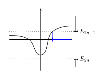
Figure 2. Examples of $W$ for which assumption (H5) holds.

Let us now shortly discuss these assumptions. One easily convinces oneself that, if (H5) or (H6) holds for some energy $E_{0}$, it will hold for all real energies in a neighborhood of $E_{0}$. Moreover, the fact that the sets $U_{-}(E)$ or $U_{+}(E)$ in the decomposition of $\mathcal{W}(E)\cap{\mathbb{R}}$ are empty will not depend on $E$ (in this neighborhood). Fig. 2 provides examples where assumption (H5) holds. Under assumption (H6), Fig. 2 provides some examples where both $U_{-}(E)$ and $U_{+}(E)$ are non empty, and Fig. 3, examples where either $U_{-}(E)$ or $U_{+}(E)$ is empty. The two assumptions (H5) and (H6) correspond to the simplest possible cases: in the general case, i.e. when the sets $E-W({\mathbb{R}})$ and $\sigma(H_{0})$ are in a general position, there can be more than one compact connected component to the set $\{\zeta\in{\mathbb{R}};\ E-W(\zeta)\in\sigma(H_{0})\}$.

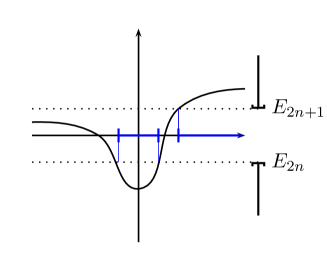
Figure 3. Examples for which assumption (H6) holds and either $U_{-}$ or $U_{+}$ is empty

We now state our results on the resonances of $H_{\zeta,\varepsilon}$.

1.4. Resonance free regions

We begin our results with the energies a neighborhood of which do not carry resonances, namely the energies satisfying (H5). Indeed, we prove

Theorem 1.2 ([16]).

Fix $E_{0}$ satisfying (H5). There exist $\varepsilon_{0}>0$, $\delta_{0}>0$, $V_{0}\subset{\mathbb{C}}$, a neighborhood of $E_{0}$ such that, for $\varepsilon\in(0,\varepsilon_{0})$, for all real $\zeta$, the set $V_{0}$ contains no resonance of $H_{\zeta,\varepsilon}$.

This is quite analogous to what is found in the case when $H_{0}$ is the free Laplace operator (see e.g. [14, 15]).

1.5. Computing the resonances

To study the real energies close to which one finds resonances, we introduce a few auxiliary functions necessary to describe the resonances.

1.5.1. The complex momentum and its branch points

The complex momentum $\zeta\mapsto\kappa(\zeta)$ is defined by

(1.2) $$\kappa(\zeta)=\kappa(\zeta,E)=k(E-W(\zeta)).$$

As $k$, $\kappa$ is analytic and multi-valued. As the branch points of $k$ are the points $(E_{i})_{i\in{\mathbb{N}}}$, the branch points of $\kappa$ satisfy

(1.3) $$E-W(\zeta)=E_{j},\ j\in{\mathbb{N}}^{*}.$$

As $E$ is real, the set of these points is symmetric with respect to the real axis, to the imaginary axis and it is $2\pi$-periodic in $\zeta$. More details are given in section 2.2.1.
Fix $E_{0}$ satisfying assumption (H6). By (1.3), for $E$ real close to $E_{0}$, the ends of $U(E)$ and the finite ends of $U_{-}(E)$ and $U_{+}(E)$ (when they are not empty) are branch points of $\kappa$. To fix ideas, let us define

$$U(E)=[\zeta_{0}^{-}(E),\zeta_{0}^{+}(E)],\quad U_{-}(E)=(-\infty,\zeta^{-}(E)]\quad\text{and}\quad U_{+}(E)=[\zeta^{+}(E),+\infty)$$

When $U_{+}(E)$ (resp. $U_{-}(E)$) is empty, we set $\zeta^{+}(E)=+\infty$ (resp. $\zeta^{-}(E)=-\infty$).
One shows that there exists a determination of the complex momentum, say $\kappa_{0}$, and a real neighborhood of $E_{0}$, say $V_{0}^{\mathbb{R}}$, such that, for $E\in V_{0}^{\mathbb{R}}$, $\kappa_{0}(\zeta)\in[0,\pi]$ for $\zeta\in U(E)$. One defines

(1.4) $$\Phi_{0}(E)=\int_{\zeta_{0}^{-}(E)}^{\zeta_{0}^{+}(E)}\kappa_{0}(\zeta,E)d\zeta\quad\text{and}\quad\delta\kappa=\frac{1}{\pi}[\kappa(\zeta_{0}^{+}(E),E)-\kappa_{0}(\zeta_{0}^{-}(E),E)].$$

One shows

Lemma 1.1 ([16]).

The constant $\delta\kappa$ belongs to $\{-1,1,0\}$ and is independent of $E$ in $V_{0}^{\mathbb{R}}$. The function $\Phi_{0}:\ V_{0}^{\mathbb{R}}\to{\mathbb{R}}^{+}$ can be extended to a function analytic in a complex neighborhood of $E_{0}$. Moreover, there exists $C>0$ such that, in this neighborhood, one has

(1.5) $$|\Phi^{\prime}_{0}(E)|\geq\frac{1}{C}\quad\text{and}\quad\Phi^{\prime}_{0}(E)\cdot\delta\kappa\geq 0.$$

Assume $U_{-}(E)$ or $U_{+}(E)$ or both are not empty. One then proves that the imaginary part of the determination $\kappa_{0}$ keeps a fixed sign in the interval between $U_{-}(E)$ and $U(E)$, and between $U(E)$ and $U_{+}(E)$, i.e. on the intervals $(\zeta_{-}(E),\zeta_{0}^{-}(E))$ and $(\zeta_{0}^{+}(E),\zeta_{+}(E))$. We define

(1.6) $$S_{-}(E)=\pm\int_{\zeta_{-}(E)}^{\zeta_{0}^{-}(E)}\text{Im}\,\kappa(\zeta)d\zeta\quad\left(\text{resp.}\quad S_{+}(E)=\pm\int_{\zeta_{0}^{+}(E)}^{\zeta_{+}(E)}\text{Im}\,\kappa(\zeta)d\zeta\right)$$

where $\pm$ is chosen so that $S_{+}(E)$ and $S_{-}(E)$ are positive. One proves

Lemma 1.2 ([16]).

Pick $\nu\in\{+,-\}$. The function $S_{\nu}:\ V_{0}^{\mathbb{R}}\to{\mathbb{R}}^{+}$ can be extended to a function analytic in a complex neighborhood of $E_{0}$.

When $U_{+}(E_{0})$ (resp. $U_{-}(E_{0})$) is empty, it stays empty for $E$ close to $E_{0}$, and one sets $S_{+}(E)=+\infty$ (resp. $S_{-}(E)=+\infty$). Define the tunneling coefficients

(1.7) $$t_{\pm}(E)=e^{-S_{\pm}(E)/\varepsilon}\quad\text{and}\quad t(E)=t_{+}(E)+t_{-}(E).$$

1.5.2. Resonances

We prove

Theorem 1.3 ([16]).

Fix $E_{0}$ satisfying (H6). There exist $\varepsilon_{0}>0$, $\delta_{0}>0$, $V_{0}\subset{\mathbb{C}}$, a neighborhood of $E_{0}$, and a real analytic function $E\mapsto\check{\Phi}(E,\varepsilon)$ defined on $V_{0}\times[0,\varepsilon_{0}]$ satisfying the uniform asymptotics

(1.8) $$\check{\Phi}(E,\varepsilon)=\Phi(E)+O(\varepsilon)\quad\text{when }\varepsilon\to 0,$$

such that, if one defines the finite sequence of points in $V_{0}\cap{\mathbb{R}}$, say $(E^{l})_{l}:=(E^{l}(\zeta,\varepsilon))_{l}$, by

(1.9) $$\frac{1}{\varepsilon}\check{\Phi}(E^{l},\varepsilon)=\frac{1}{\varepsilon}\pi\,\delta\kappa\,\zeta+\frac{\pi}{2}+\pi l,\quad l\in{\mathbb{Z}},$$

then, for $\varepsilon\in(0,\varepsilon_{0})$, for all real $\zeta$, the resonances of $H_{\zeta,\varepsilon}$ in $V_{0}$ are contained in the union of the disks

(1.10) $$D^{l}:=\left\{E\in V_{0};\ |E-E^{l}|\leq e^{-\delta_{0}/\varepsilon}\right\}.$$

More precisely, each of these disks contains exactly one simple resonance, say $\tilde{E}^{l}(\zeta,E)$, that satisfies

(1.11) $$\text{Im}\,(\tilde{E}^{l}(\zeta,E))=\varepsilon\cdot c_{0}\cdot t(E^{l})(1+o(1))$$

where $o(1)\to 0$ when $\varepsilon\to 0$ and $c_{0}$ is a constant.

Let us discuss the resonances obtained in Theorem 1.3, in particular, their behavior as functions of $\zeta$. By Theorem 1.1, the function $\zeta\mapsto\Delta(E,\zeta,\varepsilon)$ is $\varepsilon$-periodic and by Theorem 1.3, the resonances are simple, the resonances being the zeroes of $E\mapsto\Delta(E,\zeta,\varepsilon)$, they are $\varepsilon$-periodic functions of $\zeta$.

Theorem 1.3 says that their imaginary part does not oscillate to first order. It also gives some information about the oscillations of the real part. Therefore one has to distinguish the two cases $\delta\kappa\not=0$ and $\delta\kappa=0$.

When $\delta\kappa\not=0$, the quantization condition (1.9) and equations (1.5) and (1.9) show that the real part of the resonances is monotonous in $\zeta$. But, as they come in a sequence, renumbering the resonances, they can also be seen as oscillating with amplitude roughly $C\varepsilon$ (for $C>0$). Of course, to see this oscillation phenomenon, one needs to renumber the resonances. The situation is similar to that encountered when studying Stark-Wannier resonances (see [1]); in this case also, the resonances still exhibit oscillations of frequency $2\pi/\varepsilon$ but the amplitude is $\varepsilon$ (the Stark-Wannier ladders).

When $\delta\kappa\not=0$, Theorem 1.3 shows that the oscillations of the real part are at most exponentially small. Under more precise assumption than those made in the present talk, one can compute the amplitude of the oscillations of the resonances ([17]). An analogous behavior was found for the eigenvalues of $H_{\zeta,\varepsilon}$ outside the essential spectrum in [20]; they oscillate with a frequency $2\pi/\varepsilon$ and an amplitude that is exponentially small in $\varepsilon$; the amplitude was given by a complex tunneling coefficient.

Moving the energy $E$ (for a fixed $W$), one sees that, in some cases, one can pass continuously from assumption (H5) to (H6) and vice-versa. It would be interesting to study what happens to the resonances uncovered in Theorem 1.3 when one crosses this transition. Such a study has been done in [12, 13] in the case when $V\equiv 0$.

1.6. The heuristics

We now discuss the heuristics explaining these results. In the figures below, in the part indexed a), we represented the local configurations of the potential to show the assumption made on the energy $E$ in the different cases. In the part indexed b), we represented the phase space picture of the iso-energy curve i.e. the sets $\{(\kappa,\zeta)\in{\mathbb{R}}^{2};\ \kappa=\kappa(E-W(\zeta))\}$. It is $2\pi$-periodic in the $\kappa$-direction (i.e. the vertical direction) so we depicted only two periods.

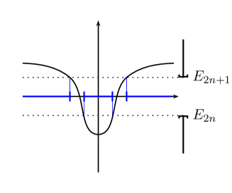
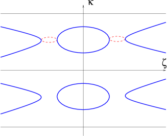
Figure 4. The phase space picture

On the same picture, we also show some loops that are dashed. These are special loops in $\{(\kappa,\zeta)\in{\mathbb{C}}^{2};\ \kappa=\kappa(E-W(\zeta))\}$ that join the connected components of $\{(\kappa,\zeta)\in{\mathbb{R}}^{2};\ \kappa=\kappa(E-W(\zeta))\}$.
Assumption (H5) just means that the real iso-energy curve is empty, in which case there are no resonances as we saw. We now assume (H6) holds.

In Fig. 4, the compact connected components of the iso-energy curve consist of a single torus per periodicity cell. The torus gives rise to the quantization condition (1.8): the corresponding phase is obtained (to first order) by integrating the canonical one-form $\kappa d\zeta$ along this torus. The fact that this corresponds to a resonance rather than to a eigenvalue is due to the fact that the iso-energy curve has components leading to infinity. The dashed curve represents the instanton linking the two. To compute the action determining the lifetime of the resonance, one integrates the canonical one-form $\kappa d\zeta$ along this curve.

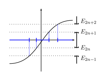
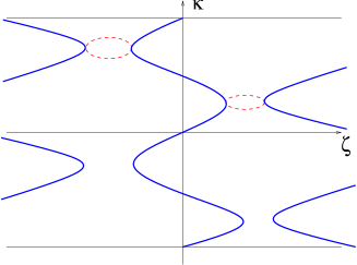
Figure 5. The phase space picture

In Fig. 5, the compact connected components of the iso-energy curve are absent. Nevertheless, one can compute a phase (to first order) by integrating the canonical one-form $\kappa d\zeta$ along a period of the central curve i.e. the one that is extended in the $\kappa$-direction. When the connected component extended in the $\zeta$-directions are absent, one can show that such a phase does not give rise to eigenvalues. The presence of these components leading to infinity in the $\zeta$-direction gives rise to resonances. Again, to compute the action determining the lifetime of the resonance, one integrates the canonical one-form $\kappa d\zeta$ along the dashed curve.

2. The adiabatic complex WKB method and the proof of Theorem 1.1

In [6] and [8], we have developed a new asymptotic method to study solutions to an adiabatically perturbed periodic Schrödinger equation i.e., to study solutions of the equation

(2.1) $$-\frac{d^{2}}{dx^{2}}\psi(x,\zeta)+(V(x)+W(\varepsilon x+\zeta))\psi(x,\zeta)=E\psi(x,\zeta)$$

in the limit $\varepsilon\to 0$. The function $\zeta\mapsto W(\zeta)$ is an analytic function in a neighborhood of the real axis. The main idea of the method is to get the information on the behavior of the solutions in $x$ from the study of their behavior on the complex plane of $\zeta$. The natural condition allowing to relate the behavior in $\zeta$ to the behavior in $x$ is the consistency condition

(2.2) $$\psi(x+1,\,\zeta,E)=\psi(x,\,\zeta+\varepsilon,E).$$

One can construct solutions to both (2.1) and (2.2) that have a simple asymptotic behavior on certain domains of the complex plane of $\zeta$.
The ideas underlying this result are simple. For solutions of (2.1) satisfying (2.2), it is equivalent to know their behavior for large $x$ or for large $\zeta$. Hence, the idea is to study their behavior for large $\zeta$. Keeping $x$ fixed to some compact interval, say $[-1,1]$, to first order in $\varepsilon$, a solution to (2.1) is a solution to

(2.3) $$-\frac{d^{2}}{dx^{2}}\psi\,(x)+V\,(x)\psi\,(x)=\mathcal{E}\psi\,(x),\quad x\in{\mathbb{R}},$$

for $\mathcal{E}=E-W(\zeta)$. Hence, the Bloch solutions are special solutions to this equation. From these solution, multiplying them by a suitably chosen function of $\zeta$ (i.e. independent of $x$), one can construct solution to both (2.1) and (2.2) at the same time. The standard form of the solutions is given below in (2.11).

We first describe the standard asymptotic behavior of consistent solutions; in order to do this, we recall some fact on periodic Schrödinger operators on ${\mathbb{R}}$. Then, we review the theory developed in [6, 8] on the existence of consistent solutions with these asymptotics. We next describe some new results used to control the behavior of the solutions at infinity. We conclude this section with the proof of Theorem 1.1.

2.1. Periodic Schrödinger operators

In this section, we discuss the periodic Schrödinger operator (0.2) where $V$ is a $1$-periodic, real valued, $L^{2}_{loc}$-function. First, we collect well known results needed in the present paper (see [11, 5, 18, 21, 23]). In the second part of the section, we introduce a meromorphic differential defined on the Riemann surface associated to the periodic operator. This object plays an important role for the adiabatic constructions (see [8]).

2.1.1. Bloch solutions

Let $\psi$ be a nontrivial solution of the equation (2.3) satisfying the relation $\psi\,(x+1)=\lambda\,\psi\,(x)$ for all $x\in{\mathbb{R}}$ with $\lambda\in{\mathbb{C}}$ independent of $x$. Such a solution is called a Bloch solution, and the number $\lambda$ is called the Floquet multiplier. We now discuss properties of Bloch solutions (see [11]).

As in section 1.1, we denote the spectral bands of the periodic Schrödinger equation by $[E_{1},\,E_{2}]$, $[E_{3},\,E_{4}]$, $\dots$, $[E_{2n+1},\,E_{2n+2}]$, $\dots$. Consider $\mathcal{S}_{\pm}$, two copies of the complex plane $\mathcal{E}\in{\mathbb{C}}$ cut along the spectral bands. Paste them together to get a Riemann surface with square root branch points. We denote this Riemann surface by $\mathcal{S}$. In the sequel, $\pi_{c}:\ {\mathcal{S}}\mapsto{\mathbb{C}}$ is the canonical projection.

One can construct a Bloch solution $\psi(x,\mathcal{E})$ of equation (2.3) meromorphic on $\mathcal{S}$. For any $\mathcal{E}$, we normalize it by the condition $\psi(1,\mathcal{E})=1$. Then, the poles of $\mathcal{E}\mapsto\psi(x,\mathcal{E})$ are projected by $\pi_{c}$ either in the open spectral gaps or at their ends. More precisely, there is exactly one simple pole per open gap. The position of the pole is independent of $x$ (see [11]).

Let $\hat{\cdot}:\ {\mathcal{S}}\mapsto{\mathcal{S}}$ be the canonical transposition mapping: for any point $\mathcal{E}\in\mathcal{S}$, the point $\hat{\mathcal{E}}$ is the unique solution to the equation $\pi_{c}(\mathcal{E})=E$ different from $\mathcal{E}$ outside the branch points.
The function $x\mapsto\psi(x,{\hat{\mathcal{E}}})$ is one more Bloch solution of (2.3). Except at the edges of the spectrum (i.e. the branch points of $\mathcal{S}$), the functions $\psi(\cdot,{\mathcal{E}})$ and $\psi(\cdot,\hat{\mathcal{E}})$ are linearly independent solutions of (2.3). In the spectral gaps, they are real valued functions of $x$, and, on the spectral bands, they differ only by the complex conjugation (see [11]).

2.1.2. The Bloch quasi-momentum

Consider the Bloch solution $\psi(x,\mathcal{E})$. The corresponding Floquet multiplier $\lambda\,(\mathcal{E})$ is analytic on $\mathcal{S}$. Represent it in the form $\lambda(\mathcal{E})=\exp(ik(\mathcal{E}))$. The function $k(\mathcal{E})$ is the Bloch quasi-momentum.
The Bloch quasi-momentum is an analytic multi-valued function of $\mathcal{E}$. It has the same branch points as $\psi(x,\mathcal{E})$ (see [11]).
Let $D\in{\mathbb{C}}$ be a simply connected domain containing no branch point of the Bloch quasi-momentum $k$. On $D$, fix $k_{0}$, a continuous (hence, analytic) branch of $k$. All other branches of $k$ that are continuous on $D$ are then given by the formula

$$k_{\pm,l}({\mathcal{E}})=\pm k_{0}({\mathcal{E}})+2\pi l,\quad l\in{\mathbb{Z}}.$$

All the branch points of the Bloch quasi-momentum are of square root type: let $E_{l}$ be a branch point, then, in a sufficiently small neighborhood of $E_{l}$, the quasi-momentum is analytic as a function of the variable $\sqrt{\mathcal{E}-E_{l}}$; for any analytic branch of $k$, one has

$$k(\mathcal{E})=k_{l}+c_{l}\sqrt{\mathcal{E}-E_{l}}+O(\mathcal{E}-E_{l}),\quad c_{l}\not=0,$$

with constants $k_{l}$ and $c_{l}$ depending on the branch.
Let ${\mathbb{C}}_{+}$ be the upper complex half-plane. There exists $k_{p}$, an analytic branch of $k$ that conformally maps ${\mathbb{C}}_{+}$ onto the quadrant $\{k\in{\mathbb{C}};\ {\rm Im}\,k>0,\,\,{\rm Re}\,k>0\}$ cut along compact vertical intervals, say $\pi l+iI_{l}$ where $l\in{\mathbb{N}}^{*}$ and $I_{l}\subset{\mathbb{R}}$, (see [11]). The branch $k_{p}$ is continuous up to the real line. It is real and increasing along the spectrum of $H_{0}$; it maps the spectral band $[E_{2n-1},E_{2n}]$ on the interval $[\pi(n-1),\pi n]$. On the open gaps, ${\rm Re}\,k_{p}$ is constant, and ${\rm Im}\,k_{p}$ is positive and has exactly one maximum; this maximum is non degenerate.
We call $k_{p}$ the main branch of the Bloch quasi-momentum.
Finally, we note that the main branch can be analytically continued on the complex plane cut only along the spectral gaps of the periodic operator.

2.1.3. Meromorphic differential $\Omega$

On the Riemann surface $\mathcal{S}$, consider the function

(2.4) $$\omega({\mathcal{E}})=-\frac{\int_{0}^{1}\psi(x,\hat{\mathcal{E}})\,\left(\dot{\psi}(x,{\mathcal{E}})-i\dot{k}({\mathcal{E}})x\,\psi(x,{\mathcal{E}})\right)\,dx}{\int_{0}^{1}\psi(x,{\mathcal{E}})\psi(x,\hat{\mathcal{E}})dx}.$$

where $k$ is the Bloch quasi-momentum of $\psi$, and the dot denotes the partial derivative with respect to ${\mathcal{E}}$. This function was introduced in [10] (the definition given in that paper is equivalent to (2.4)). In [10], we have proved that $\omega$ has the following properties:

1. the differential $\Omega=\omega\,d{\mathcal{E}}$ is meromorphic on $\mathcal{S}$; its poles are the points of $P\cup Q$, where $P$ is the set of poles of $\psi(x,{\mathcal{E}})$, and $Q$ is the set of points where $k^{\prime}({\mathcal{E}})=0$;

2. all the poles of $\Omega$ are simple;

3. $\forall p\in P\setminus Q$, ${\rm res}\,_{p}\Omega=1$; $\forall q\in Q\setminus P$, ${\rm res}\,_{q}\Omega=-1/2$; $\forall r\in P\cap Q$, ${\rm res}\,_{r}\Omega=1/2$.

4. if $\pi_{c}({\mathcal{E}})$ belongs to a gap, then $\omega({\mathcal{E}})\in{\mathbb{R}}$;

5. if $\pi_{c}({\mathcal{E}})$ belongs to a band, then $\overline{\omega({\mathcal{E}})}=\omega(\hat{\mathcal{E}})$.

2.2. Standard behavior of consistent solutions

We now discuss in more detail two analytic objects central to the complex WKB method, the complex momentum defined in (1.2) and the canonical Bloch solutions defined below. For $\zeta\in\mathcal{D}(W)$, the domain of analyticity of the function $W$, we define

(2.5) $${\mathcal{E}}(\zeta)=E-W(\zeta)$$

The complex momentum and the canonical Bloch solutions are the Bloch quasi-momentum and particular Bloch solutions of the equation

(2.6) $$-\frac{d^{2}}{dx^{2}}\psi+V\psi={\mathcal{E}}(\zeta)\psi.$$

considered as functions of $\zeta$.

2.2.1. The complex momentum

For $\zeta\in\mathcal{D}(W)$, the domain of analyticity of the function $W$, the complex momentum is given by the formula $\kappa(\zeta)=k(\mathcal{E}(\zeta))$ where $k$ is the Bloch quasi-momentum of (0.2). Clearly, $\kappa$ is a multi-valued analytic function; a point $\zeta$ such that $W^{\prime}(\zeta)\neq 0$ is a branch point of $\kappa$ if and only if it satisfies (1.3). All the branch points of the complex momentum are of square root type.

A simply connected set $D\subset\mathcal{D}(W)$ containing no branch points of $\kappa$ is called regular. Let $\kappa_{p}$ be a branch of the complex momentum analytic in a regular domain $D$. All the other branches analytic in $D$ are described by

(2.7) $$\kappa_{m}^{\pm}=\pm\kappa_{p}+2\pi m\quad\text{where}\quad m\in{\mathbb{Z}}.$$

2.2.2. Canonical Bloch solutions

To describe the asymptotic formulae of the complex WKB method, one needs Bloch solutions of equation (2.6) analytic in $\zeta$ on a given regular domain. We build them using the 1-form $\Omega=\omega\,d\mathcal{E}$ introduced in section 2.1.3.

Pick $\zeta_{0}$, a regular point i.e. a point that is not a branch point of $\kappa$. Let $\mathcal{E}_{0}=\mathcal{E}(\zeta_{0})$. Assume that $\mathcal{E}_{0}\not\in P\cup Q$ (the sets $P$ and $Q$ are defined in section 2.1.3). In $U_{0}$, a sufficiently small neighborhood of $\mathcal{E}_{0}$, we fix $k$, a branch of the Bloch quasi-momentum, and $\psi_{\pm}(x,\mathcal{E})$, two branches of the Bloch solution $\psi(x,\mathcal{E})$ such that $k$ is the Bloch quasi-momentum of $\psi_{+}$. Also, in $U_{0}$, consider $\Omega_{\pm}$, the two corresponding branches of $\Omega$, and fix a branch of the function $\mathcal{E}\mapsto q(\mathcal{E})=\sqrt{k^{\prime}(\mathcal{E})}$. Assume that $V_{0}$ is a neighborhood of $\zeta_{0}$ such that ${\mathcal{E}}(V_{0})\subset U_{0}$. For $\zeta\in V_{0}$, we let

(2.8) $$\Psi_{\pm}(x,\zeta)=q(\mathcal{E})\,e^{\int_{\mathcal{E}_{0}}^{\mathcal{E}}\Omega_{\pm}}\psi_{\pm}(x,\mathcal{E}),\quad\text{where}\quad\mathcal{E}=\mathcal{E}(\zeta).$$

The functions $\Psi_{\pm}$ are the canonical Bloch solutions normalized at the point $\zeta_{0}$. The quasi-momentum associated to these solutions is $\kappa(\zeta)=k(E-W(\zeta))$.

The properties of the differential $\Omega$ imply that the solutions $\Psi_{\pm}$ can be analytically continued from $V_{0}$ to any regular domain $D$ containing $V_{0}$.
One has (see [6])

(2.9) $$w(\Psi_{+}(\cdot,\zeta),\Psi_{-}(\cdot,\zeta))=w(\Psi_{+}(\cdot,\zeta_{0}),\Psi_{-}(\cdot,\zeta_{0}))=k^{\prime}(\mathcal{E}_{0})w(\psi_{+}(\cdot,\mathcal{E}_{0}),\psi_{-}(\cdot,\mathcal{E}_{0}))$$

As $\mathcal{E}_{0}\not\in Q\cup\{E_{l},\ l\geq 1\}$, the Wronskian $w(\Psi_{+}(\cdot,\zeta),\Psi_{-}(\cdot,\zeta))$ does not vanish.

2.2.3. Solutions having standard asymptotic behavior

Fix $E=E_{0}$. Let $D$ be a regular domain. Fix $\zeta_{0}\in D$ so that $\mathcal{E}(\zeta_{0})\not\in P\cup Q$. Let $\kappa$ be a branch of the complex momentum continuous in $D$, and let $\Psi_{\pm}$ be the canonical Bloch solutions defined on $D$, normalized at $\zeta_{0}$ and indexed so that $\kappa$ be the quasi-momentum for $\Psi_{+}$.
We recall the following basic definition from [8]

Definition 2.1.

Fix $\eta\in\{+,-\}$, $\zeta_{0}\in D$, $X>1$, $V_{0}$, a complex neighborhood of some energy $E_{0}$ and $D$ a domain in the $\zeta$-plane. We say that $f$, a solution of (2.1), has standard asymptotics (or standard behavior) $f\sim\exp(\eta\frac{i}{\varepsilon}\int_{\zeta_{0}}^{\zeta}\kappa\,du)\cdot\Psi_{\eta}$ in $(-X,X)\times D\times V_{0}$ if

• $f$ is defined and satisfies (2.1) and (2.2) for any $(x,\zeta,E)\in(-X,X)\times D\times V_{0}$;

• $f$ is analytic in $\zeta\in D$ and in $E\in V_{0}$;

• for any $K$, compact subset of $D$, there exists $V\subset V_{0}$, a neighborhood of $E_{0}$, such that, for $(x,\zeta,E)\in(-X,X)\times K\times V$, $f$ has the uniform asymptotics

  $$f(x,\zeta,E,\varepsilon)=e^{\textstyle\eta\,\frac{i}{\varepsilon}\int_{\zeta_{0}}^{\zeta}\kappa(u,E)\,du}\,(\Psi_{\eta}(x,\zeta,E)+g_{\eta}(x,\zeta,E,\varepsilon))$$

  where

  $$\lim_{\varepsilon\to 0}\ \sup_{\begin{subarray}{c}x\in(-X,X)\\ \zeta\in K\\ E\in V\end{subarray}}|g_{\eta}(x,\zeta,E,\varepsilon)|=0.$$

• this asymptotic can be differentiated once in $x$.

Let $(f_{+},f_{-})$ be two solutions of (2.1) having standard behavior $f_{\pm}\sim e^{\textstyle\pm\frac{i}{\varepsilon}\int^{\zeta}\kappa\,d\zeta}\,\Psi_{\pm}$ in $(-X,X)\times D\times V_{0}$. One computes

$$w(f_{+},f_{-})=w(\Psi_{+},\Psi_{-})+o(1).$$

By (2.9), for $\zeta$ in any fixed compact subset of $D$ and $\varepsilon$ sufficiently small, the solutions $(f_{+},f_{-})$ are linearly independent.

2.3. The main theorem of the adiabatic complex WKB method

A basic and important example of a domain where one can construct a solution with standard asymptotic behavior is a canonical domain. Let us define canonical domains and formulate the basic result of the adiabatic complex WKB method.

2.3.1. Canonical lines

We recall that a curve $\gamma$ is vertical if it intersects the lines $\{{\rm Im}\,\zeta={\rm Const}\}$ at non-zero angles $\theta$,  $0<\theta<\pi$. Vertical lines are naturally parametrized by ${\rm Im}\,\zeta$.
A set $D$ in the $\zeta$-plane is said to be bounded regular at energy $E_{0}$ if $\overline{D}$, the closure of $D$, is compact and does not contain any branch point of $\zeta\mapsto\kappa(\zeta,E_{0})$.

Let $\gamma$ be a $C^{1}$ bounded regular vertical curve at energy $E_{0}$. On $\gamma$, fix a point $\zeta_{0}$ and $\kappa$, a continuous branch of the complex momentum.

Definition 2.2.

The curve $\gamma$ is canonical with respect to $\kappa$ at energy $E_{0}$ if, along $\gamma$, for $y={\rm Im}\,\zeta$, one has

$$\frac{d}{dy}\,{\rm Im}\,\left(\int_{\zeta_{0}}^{\zeta}\kappa(u,E_{0})du\right)>0\quad\text{and}\quad\frac{d}{dy}\,\left({\rm Im}\,\int_{\zeta_{0}}^{\zeta}(\kappa(u,E_{0})-\pi)du\right)<0$$

One easily checks that,

• if a vertical curve is bounded regular at energy $E_{0}$, it is bounded regular at any energy $E$ in a neighborhood of $E_{0}$;

• if a vertical curve is bounded regular and canonical with respect to $\kappa$ at energy $E_{0}$, it is also canonical with respect to $\kappa$ at any energy $E$ in a neighborhood of $E_{0}$.

2.3.2. Canonical domains

Let $K$ be a bounded regular domain at energy $E_{0}$ i.e. $\overline{K}$ is compact and does not contain any branch point of $\zeta\mapsto\kappa(\zeta,E_{0})$. On $K$, fix a continuous branch of the complex momentum, say $\kappa$.

Definition 2.3.

The domain $K$ is called canonical (with respect to $\kappa$ at energy $E_{0}$) if there exists two points $\zeta_{1}$ and $\zeta_{2}$ located on $\partial K$, the boundary of $K$, such that $K$ is the union of curves connecting $\zeta_{1}$ and $\zeta_{2}$ that are canonical (with respect to $\kappa$ at energy $E_{0}$).

2.3.3. The main theorem of the adiabatic complex WKB theory

One has

Theorem 2.1 ([6, 8]).

Let $K$ be a bounded domain canonical with respect to $\kappa$ at energy $E_{0}$. Fix $X>1$ and $\zeta_{0}\in K$. Then, there exists $V_{0}$, a neighborhood of $E_{0}$ such that, for sufficiently small positive $\varepsilon$, there exist $(f_{\pm})$, two solutions of (0.1), having the standard behavior in $(-X,X)\times K\times V_{0}$ that is

$$f_{\pm}\sim\exp\left(\pm\frac{i}{\varepsilon}\int_{\zeta_{0}}^{\zeta}\kappa d\zeta\right)\Psi_{\pm}.$$

For any fixed $x\in{\mathbb{R}}$, the functions $(\zeta,E)\mapsto f_{\pm}(x,\zeta,E)$ are analytic in $S(K)\times V_{0}$ where $S(K)$ is the smallest horizontal strip containing $K$.

In addition to this result, we need analogues for domains that are neighborhoods of infinity. Such results were developed in [19, 20]; they are not sufficient for the purpose of the present paper. Hence, we present two new results in the next section.

2.4. Consistent solutions at infinity

The standard behavior at infinity is given by

Theorem 2.2 ([16]).

Assume (H1)-(H4) are satisfied. Fix $\eta\in\{+,-\}$ and $\alpha\in(0,1)$. Pick $E_{0}\in{\mathbb{R}}$ such that either $E_{0}-W_{\eta}\in\sigma(H_{0})\setminus\partial\sigma(H_{0})$. Fix $X>1$ and $C_{1}>C_{0}$ (where $C_{0}$ is defined in assumption (H4), section 1.2). Then, there exist $C>0$ and $\delta>0$ such that, for any $E\in D(E_{0},\delta)$, the cone $\mathcal{C}_{\eta}=\{\zeta\in{\mathbb{C}};\ \eta\text{Re}\,\zeta>C,\ C_{1}|\text{Im}\,\zeta|<\eta\text{Re}\,\zeta\}$ is a canonical domain. More precisely, fix $\zeta_{0}\in\mathcal{C}_{\eta}\cap{\mathbb{R}}$. Then, there exist a branch of the quasi-momentum $\kappa(\zeta)=\kappa(\zeta,E)$ that satisfies

(2.10) $$\forall(\zeta,E)\in\mathcal{C}_{\eta}\times D(E_{0},\delta),\quad 0<\text{Re}\,\kappa(\zeta,E)<\pi$$

and a function $(x,\zeta,E)\mapsto f(x,\zeta,E)$ defined on $(-X,X)\times\mathcal{C}_{\eta}\times D(E_{0},\delta)$ that satisfies:

• it is a consistent solution to equation (2.1)

• for $x\in(-X,X)$, $(\zeta,E)\mapsto f(x,\zeta,E)$ is analytic on $\mathcal{C}_{\eta}\times D(E_{0},\delta)$;

• the function $f$ admits the asymptotics

  (2.11) $$f(x,\zeta,E)=e^{\frac{i}{\varepsilon}\int_{\zeta_{0}}^{\zeta}\kappa(u,E)du}\left(\Psi(x,\zeta,E)+g(x,\zeta,E,\varepsilon)\right)$$

  where $\Psi$ is the canonical Bloch solutions $\Psi_{+}$ associated to $\kappa$ (see (2.8)) and

  (2.12) $$\sup_{\varepsilon\in(0,\varepsilon_{0})}\sup_{\begin{subarray}{c}\zeta\in\mathcal{C}_{+}\\ E\in D(E_{0},\delta)\end{subarray}}|\varepsilon^{\alpha-1}\zeta^{s}g(x,\zeta,E,\varepsilon)|<+\infty.$$

• the asymptotics can be differentiated once in $x$;

• define the function $(x,\zeta,E)\mapsto f^{*}(x,\zeta,E)=\overline{f(\overline{x},\overline{\zeta},\overline{E})}$ ; then, $(f,f^{*})$ form a basis of consistent solutions and satisfy

  (2.13) $$w(f(\cdot,\zeta,E),f^{*}(\cdot,\zeta,E))=w(\Psi_{+}(\cdot,\zeta_{0}),\Psi_{-}(\cdot,\zeta_{0})).$$

We will use a second result concerning consistent solutions near $\infty$. We won’t need a basis in this case: a single solution (actually the Jost solution) will be sufficient. It is given by

Theorem 2.3 ([16]).

Assume (H1)-(H4) are satisfied. Fix $\eta\in\{+,-\}$ and $\alpha\in(0,1)$. Pick $E_{0}\in{\mathbb{R}}$ such that $E_{0}-W_{\eta}\not\in\sigma(H_{0})$. Fix $X>1$ and $C_{1}>C_{0}$ (where $C_{0}$ is defined in assumption (H4), section 1.2). Then, there exist $C>0$ and $\delta>0$ such that, for any $E\in D(E_{0},\delta)$, the cone $\mathcal{C}_{\eta}=\{\zeta\in{\mathbb{C}};\ \eta\text{Re}\,\zeta>C,\ C_{1}|\text{Im}\,\zeta|<\eta\text{Re}\,\zeta\}$ is a canonical domain. More precisely, fix $\zeta_{0}\in\mathcal{C}_{\eta}\cap{\mathbb{R}}$. Then, there exist a branch of the quasi-momentum $\kappa(\zeta)=\kappa(\zeta,E)$ that satisfies, for some $\sigma\in\{0,1\}$,

(2.14) $$\forall(\zeta,E)\in\mathcal{C}_{\eta}\times D(E_{0},\delta),\quad 0<\text{Im}\,\kappa(\zeta,E)\quad\text{and}\quad\kappa^{*}(\zeta,E)=2\pi\sigma-\kappa(\zeta,E).$$

and a function $(x,\zeta,E)\mapsto f(x,\zeta,E)$ defined on $(-X,X)\times\mathcal{C}_{\eta}\times D(E_{0},\delta)$ that satisfies:

• $f$ is a consistent solution to equation (2.1)

• for $x\in(-X,X)$, $(\zeta,E)\mapsto f(x,\zeta,E)$ is analytic on $\mathcal{C}_{\eta}\times D(E_{0},\delta)$;

• the function $f$ admits the asymptotics

  (2.15) $$f(x,\zeta,E)=e^{\eta\frac{i}{\varepsilon}\int_{\zeta_{0}}^{\zeta}\kappa(u,E)du}\left(\Psi_{\eta}(x,\zeta,E)+g(x,\zeta,E,\varepsilon)\right)$$

  where $(\Psi_{+},\Psi_{-})$ are the canonical Bloch solutions associated to $\kappa$ (see (2.8)) and $g$ satisfy (2.12);

• the asymptotics can be differentiated once in $x$;

• the functions satisfy

  (2.16) $$\forall(x,\zeta,E)\in(-X,X)\times\mathcal{C}_{\eta}\times D(E_{0},\delta),\quad f^{*}(x,\zeta,E)=e^{-2\pi\sigma\eta i(\zeta-\zeta_{0})/\varepsilon}f(x,\zeta,E).$$

In [20, 19], a result analogous to Theorem 2.3 is proved, the main difference being the region in $\zeta$ where the statements hold.

2.5. The continuation diagrams

Now to achieve the goal described in section 2, namely, to construct consistent solutions to (2.1) with known asymptotics in large complex domains of $\zeta$, as we have the form of standard asymptotics locally both at a finite point in $\zeta$ and near infinity, we only need patch together the various domain on which we found consistent basis with standard asymptotics. An alternative way to obtain global asymptotics was developed in [8, 10, 7, 9]. It consists in the proof of quite general continuation lemmas that describe geometric situations in the complex plane of $\zeta$ under which one can prove that, starting from a canonical domain and solutions with standard asymptotics in this domain, one can continue them. The main obstacles to continuation (i.e. to the validity of standard asymptotics) are the nodal lines of ${\rm Im}\,\kappa$ and the branching points of $\kappa$. We will not discuss this further and refer to [16] for the details.

References

- [1] V. Buslaev and A. Grigis. Imaginary parts of Stark-Wannier resonances. J. Math. Phys., 39(5):2520–2550, 1998.
- [2] V. Buslaev and A. Grigis. Turning points for adiabatically perturbed periodic equations. J. Anal. Math., 84:67–143, 2001.
- [3] M. Dimassi. Resonances for slowly varying perturbations of a periodic Schrödinger operator. Canad. J. Math., 54(5):998–1037, 2002.
- [4] M. Dimassi and M. Zerzeri. A local trace formula for resonances of perturbed periodic Schrödinger operators. J. Funct. Anal., 198(1):142–159, 2003.
- [5] M. Eastham. The spectral theory of periodic differential operators. Scottish Academic Press, Edinburgh, 1973.
- [6] A. Fedotov and F. Klopp. A complex WKB method for adiabatic problems. Asymptot. Anal., 27(3-4):219–264, 2001.
- [7] A. Fedotov and F. Klopp. Anderson transitions for a family of almost periodic Schrödinger equations in the adiabatic case. Comm. Math. Phys., 227(1):1–92, 2002.
- [8] A. Fedotov and F. Klopp. Geometric tools of the adiabatic complex WKB method. Asymptot. Anal., 39(3-4):309–357, 2004.
- [9] A. Fedotov and F. Klopp. On the singular spectrum for adiabatic quasi-periodic Schrödinger operators on the real line. Ann. Henri Poincaré, 5(5):929–978, 2004.
- [10] A. Fedotov and F. Klopp. On the absolutely continuous spectrum of one-dimensional quasi-periodic Schrödinger operators in the adiabatic limit. Trans. Amer. Math. Soc., 357(11):4481–4516 (electronic), 2005.
- [11] N. E. Firsova. On the global quasimomentum in solid state physics. In Mathematical methods in physics (Londrina, 1999), pages 98–141. World Sci. Publishing, River Edge, NJ, 2000.
- [12] S. Fujiié and T. Ramond. Matrice de scattering et résonances associées à une orbite hétérocline. Ann. Inst. H. Poincaré Phys. Théor., 69(1):31–82, 1998.
- [13] S. Fujiié and T. Ramond. Breit-Wigner formula at barrier tops. J. Math. Phys., 44(5):1971–1983, 2003.
- [14] B. Helffer and J. Sjöstrand. Résonances en limite semi-classique. Mém. Soc. Math. France (N.S.), (24-25):iv+228, 1986.
- [15] P. Hislop and I. Sigal. Semi-classical theory of shape resonances in quantum mechanics. Memoirs of the American Mathematical Society, 78, 1989.
- [16] F. Klopp and M. Marx. Resonances for slowly varying perturbations of one-dimensional periodic Schrödinger operators. in progress.
- [17] F. Klopp and M. Marx. Resonances for slowly varying perturbations of one-dimensional periodic Schrödinger operators II: oscillation of resonances. in progress.
- [18] V. Marchenko and I. Ostrovskii. A characterization of the spectrum of Hill’s equation. Math. USSR Sbornik, 26:493–554, 1975.
- [19] M. Marx. Étude de perturbations adiabatiques de l’équation de Schrödinger périodique. PhD thesis, Université Paris 13, Villetaneuse, 2004.
- [20] M. Marx. On the eigenvalues for slowly varying perturbations of a periodic Schrödinger operator. To appear in Asymptotic Analysis, 2006.
- [21] H. P. McKean and E. Trubowitz. Hill’s surfaces and their theta functions. Bull. Amer. Math. Soc., 84(6):1042–1085, 1978.
- [22] J. Sjöstrand. Lectures on resonances, 2002. http://www.math.polytechnique.fr/~sjoestrand/CoursgbgWeb.pdf
- [23] E.C. Titschmarch. Eigenfunction expansions associated with second-order differential equations. Part II. Clarendon Press, Oxford, 1958.
- [24] M. Zworski. Counting scattering poles. In Spectral and Scattering, volume 161 of Lecture Notes in Pure and Applied Mathematics, pages 301–331, New-York, 1994. Marcel Dekker.
- [25] M. Zworski. Quantum resonances and partial differential equations. In Proceedings of the International Congress of Mathematicians, Vol. III (Beijing, 2002), pages 243–252, Beijing, 2002. Higher Ed. Press.
- [26] M. Zworski. Resonances in physics and geometry. Notices Amer. Math. Soc., 46(3):319–328, 1999.