SOLITON-LIKE EXCITATION IN LARGE-$\alpha$ QED

Аннотация

Abstract

The nonperturbative analysis of the one-particle excitation of the electron-positron field is made in the paper. The standard form of quantum electrodynamics (QED) is used but the coupling constant $\alpha_{0}$ is supposed to be of a large value ($\alpha_{0}\gg 1$). It is shown that in this case the quasi-particle excitation can be produced together with the non-zero scalar component of the electromagnetic field. Self-consistent equations for spatially localized charge distribution coupled with an electromagnetic field are derived. Soliton-like solution with a nonzero charge for these equations are calculated numerically. The solution proves to be unique if the coupling constant is fixed. It leads to the condition of charge quantization if the non-overlapping $n$-soliton states are considered. It is also proved that the dispersion law of the soliton-like excitation is consistent with Lorentz invariance of the QED equations.

PACS: 12.20.DS, 11.10.Gh
Keywords: nonperturbative theory, quenched QED, soliton, polaron.

I Introduction

The problem of quantum electrodynamics (QED) with strong a coupling between electron-positron and electromagnetic fields (the so-called "large-$\alpha$ QED") was developed by many authors (for example, large and citation therein). QED is a physical system with well defined Hamiltonian, so the approbation of various methods for this theory is of great interest for non-perturbative analysis of actual problems of quantum chromodynamics (for example, Kleinert ,QCD and citation therein).

One of the main approaches in this field is related to the Schwinger-Dyson equation (SD). the critical value of the coupling constant $\alpha_{c}\sim 1$ separating the regions of weak and strong coupling was discovered for this equation SD . The existence of the critical point $\alpha_{c}$ could affect some observed physical phenomena as some authors considered SD1 . Actually the SD equation defines the self-energy part of the fermion propagator and results from the accurate QED equations if the corrections for the vertex function and the Green’s function of the electromagnetic field are not taken into account. This corresponds to one of the variants of "quenched QED"when the truncated Fock basis is used for the variational perturbation theory Mors . A detailed analysis of nonperturbative approaches in large-$\alpha$ QED has been recently discussed in paper large .

It is important to pay attention to the fact that the mathematical structure of the interaction operator in QED is similar in many respects to the operator of the interaction between electron and quantum field of optical phonons in the ionic crystal, the so-called problem of a large-radius "polaron"described by the Fröhlich Hamiltonian Frohlich . This situation was recently used by authors of Alex for nonperturbative mass renormalization in the framework of "quenched QED". They made the variational estimation of the functional integral for QED on the basis of Feynman’s approach to the "polaron"problem Feynmanpol .

The main effect of the strong interaction between the electron and quantum field is defined by formation of the soliton-like ("polaronic") self-localized state of the particle coupled with the classical components which are selected from the quantum field by the particle itself. It was first discovered by Pekar Pekar and investigated rigorously in the papers Bogol ,Tyablikov . It was also proved that the soliton-like excitation (SLE) corresponds to the leading term in the series of $\alpha^{-1}$ for the Fröhlich Hamiltonian Bogol . Later a lot of different forms of the quasi-particles arising as a result of a "polaronic"effect were described for many concrete physical systems.

Then the following question is of interest: could some SLE exist in the framework of "large-$\alpha$ QED"? It is important to mention that the answer to this question cannot be found on the basis of SD equation. The matter is that the integral equation for the self-energy function was introduced for the "polaron"problem by Pines Pines and it is analogous to SD equation for QED. However, it is well known polaron , that Pines equation does not allow one to describe the strong coupling limit for the "polaron"problem correctly because the bound state of the electron and phonons is not included in this equation. It appeares that the essential reconstruction of the wave function both for electron and phonon field should be taken into account in zeroth approximation directly if the series in the power of $\alpha^{-1}$ is used for describing of SLE Bogol ,Tyablikov . If the same problem is considered on the basis of the variational estimation for functional integrals some model system qualitatively different from noninteracting particles should also be used for calculating the action in zeroth approximation directly Feynmanpol . Particularly, the harmonic interaction between electron and some fictitious particle was used for the "polaron"model, that the coupling constant and the mass of this particle being considered as the variational parameters Feynmanpol .

In this paper it is shown for the first time that SLE can also be found for QED if the original coupling constant for the interaction between electromagnetic and electron-positron fields is supposed to be large $\alpha_{0}\gg 1$. As distinct from "polaron"the self-localized SLE for QED is the quasi-particle excitation of the electron-positron field corresponding to a spatial charge distribution with a non-zero integral charge coupled with a classical scalar component of the electromagnetic field separated by the same charge density (see also electron ). In the terms of "quenched QED"it corresponds to the truncated Fock basis which consists of the linear superposition of one-particle excitation of the electron-positron field, non-zero scalar field and vacuum state for the transversal photons of the electromagnetic field.

The truncation of Fock space used in this paper differs greatly from other non-perturbative approaches (see, for example, large and references therein) because of the inclusion of a strong localized scalar field. However, it should be noticed that a similar variant of the quenched QED was recently considered in the paper Hainzl on the basis of mean-field approximation. Some general theorems were proved in this paper but the calculation of some concrete characteristics of the system was not given.

It is also shown in the paper that SLE with a non-zero charge corresponds to the minimum of the energy for one-paricle excitation of the system. The characteristics of SLE are defined by self-consistent equations for electron-positron wave functions and a scalar field. The equations are derived on the basis of an operator method (OM) introduced earlier for non-perturbative description of quantum systems ( for example, OM and references therein). These results are described in $\S$ 2.

The solution of these nonlinear self-consistent equations is considered in $\S$ 3 on the basis of the numerical method developed earlier for the "polaron"problem Krylov . It is shown that a non-trivial solution of these equations exists for a unique value of SLE integral charge. It can be considered as the condition of a charge quantization similar to that which appeared due to Dirac’s monopole monopol .

The dependence of SLE energy $E(\vec{P})$ on its total momentum $\vec{P}$ is analyzed in $\S$ 3. It is well known Lifshitz that this dispersion law for any one-particle excitation should be of a relativistic form because of Lorentz-invariance of QED. The problem of the relation between the localization of electron and translational invariance of the whole system also appeared for "polaron". It was rigorously solved by authors Bogol ,Gross . They proved that the "polaron"state vector did not actually break the translational symmetry of the system because the concrete point of its localization could be arbitrary in the space quasi . As is known, the dispersion law is rather complicated for the "polaron"problem and it is very difficult to find its general form analytically because the variables describing the internal dynamics of the system are not separated from the translational variables Gross .

The calculation of $E(\vec{P})$ for QED ($\S$ 3) showed that SLE localization did not contradict Lorentz-invariance of the whole system. It is also important that SLE internal degrees of freedom are separated from the translational motion and as a result its dispersion law $E(\vec{P})$ corresponds exactly to conventional dynamics of a relativistic free particle.

II Self-consistent equations for one-particle excitation in QED

Let’s consider an exact Hamiltonian QED in the Coulomb gauge Heitler , Hainzl . This representation is most convenient for us because it extracts the electrostatic interaction which, by definition, makes the main contribution to the vacuum polarization in the strong coupling limit:

$$\hat{H}=\int d\vec{r}\{\hat{\psi}^{*}(\vec{r})[\vec{\alpha}(\vec{p}+e_{0}\hat{\vec{A}}(\vec{r}))+\beta m_{0}]\hat{\psi}(\vec{r})+e_{0}\hat{\varphi}(\vec{r})\hat{\rho}(\vec{r})-\frac{1}{2}(\vec{\nabla}\hat{\varphi}(\vec{r}))^{2}\}+$$

$$\sum_{\vec{k}\lambda}\omega(\vec{k})\hat{n}_{\vec{k}\lambda};$$

$$\hat{\rho}(\vec{r})=\frac{1}{2}[\hat{\psi}^{*}(\vec{r})\hat{\psi}(\vec{r})-\hat{\psi}(\vec{r})\hat{\psi}^{*}(\vec{r})].$$ (1)

We suppose here that the field operators are given in the Schrödinger representation, the spinor components of the electron-positron operators being defined in the standard way Heitler

$$\hat{\psi}_{\nu}(\vec{r})=\sum_{s}\int\frac{d\vec{p}}{(2\pi)^{3/2}}\{a_{\vec{p}s}u_{\vec{p}s\nu}e^{i\vec{p}\vec{r}}+b^{+}_{\vec{p}s}v_{-\vec{p}-s\nu}e^{-i\vec{p}\vec{r}}\};$$

$$\hat{\psi}^{*}_{\nu}(\vec{r})=\sum_{s}\int\frac{d\vec{p}}{(2\pi)^{3/2}}\{a^{+}_{\vec{p}s}u^{*}_{\vec{p}s\nu}e^{-i\vec{p}\vec{r}}+b_{\vec{p}s}v^{*}_{-\vec{p}-s\nu}e^{i\vec{p}\vec{r}}\}.$$ (2)

In these formulas $\vec{\alpha},\beta$ are Dirac matrixes; $u_{\vec{p}s\nu}$ and $v_{\vec{p}s\nu}$ are the components of the bispinors corresponding to the solutions of Dirac equation for the free "bare"electron and positron with the momentum $\vec{p}$ and spin s; $a_{\vec{p}s}(a^{+}_{\vec{p}s})$ and $b_{\vec{p}s}(b^{+}_{\vec{p}s})$ are the annihilation (creation) operators for the "bare"electrons and positrons in the corresponding states. The field operator $\hat{\vec{A}}(\vec{r})$ and the operator of the photon number $\hat{n}_{\vec{k}\lambda}$ are related to the transversal electromagnetic field and their explicit form will be written below. It should be remembered that the parameter $e_{0}$ was introduced as a positively defined value.

We should also discuss the dependence of the QED hamiltonian on the operator of the scalar field

$$\hat{\varphi}(\vec{r})=\sqrt{4\pi}\int d\vec{k}\hat{\varphi}_{\vec{k}}e^{i\vec{k}\vec{r}}.$$ (3)

It is knownHeitler , that these operators can be excluded from the Hamiltonian in the Coulomb gauge. For that purpose one should use the solution of the operator equations of motion for $\hat{\varphi}_{\vec{k}}$ assuming that the "bare"electrons are point-like particles and "self-action"is equivalent to the substitution of the initial mass for the renormalized one. As a result the terms with scalar fields in the Hamiltonian are reduced to the Coulomb interaction between the charged particles. However, this transformation of the hamiltonian (II) cannot be used in this paper because just the dynamics of the mass renormalization is the subject under investigation.

There is another problem connected with a negative sign of the term corresponding to the self-energy of the scalar field. If the non-relativistic problems were considered then the operator of the particle kinetic energy would be positively defined and the negative operator with the square-law dependence on $\hat{\varphi}(\vec{r})$ would lead to the "fall on the center"Landau as the energy minimum would be reached at an infinitely large field amplitude. However, if the relativistic fermionic field is considered then the operator of the free particle energy (the first term in formula (II)) is not positively defined. Besides, the states of the system with the negative energy are filled. Therefore, the stable state of the system corresponds to the energy extremum (!) (the minimum one for electron and the maximum one for positron excited states). It can be reached at the finite value of the field amplitude (see below). The same reasons enable one to successfully use the states with indefinite metric Akhiezer in QED although it leads to some difficulties in the non-relativistic quantum mechanics.

According to our main assumption about the large value of the initial coupling constant $e_{0}$ we are to realize the nonperturbative description of the excited state which is the nearest to the vacuum state of the system. The basic method for the nonperturbative estimation of the energy is the variational approach with some trial state vector $|\Phi_{1}>$ for the approximate description of the one-particle excitation. The qualitative properties of the self-consistent excitation in the strong coupling limit Pekar show that such trial vector should correspond to the general form of the wave packet formed by the one-particle excitations of the "bare"electron-positron field. Besides, the effect of polarization and the appearance of the electrostatic field $\varphi(\vec{r})$ should be taken into account, so we consider $|\Phi_{1}>$ to be the eigenvector for the operator of the scalar field. Now, let’s introduce the following trial vector depending on the set of variational classical functions $U_{\vec{q}s};V_{\vec{q}s};\varphi(\vec{r})$ for the approximate description of the quasi-particle excited state of the system:

$$|\Phi_{1}>\simeq|\Phi^{(0)}_{1}(U_{\vec{q}s};V_{\vec{q}s};\varphi(\vec{r}))>=\int d\vec{q}\{U_{\vec{q}s}a^{+}_{\vec{q}s}+V_{\vec{q}s}b^{+}_{\vec{q}s}\}|0;0;\varphi(\vec{r})>;$$

$$\hat{\varphi}(\vec{r})|0;0;\varphi(\vec{r})>=\varphi(\vec{r})|0;0;\varphi(\vec{r})>;\quad a_{\vec{q}s}|0;0;\varphi(\vec{r})>=b_{\vec{q}s}|0;0;\varphi(\vec{r})>=0.$$ (4)

The ground state of the system is $|\Phi_{0}>=|0;0;0>$, if we use the same notation. It corresponds to the vacuum of both interacting fields.

Firstly, let’s consider the excitation with the zero total momentum. Then the constructed trial vector should satisfy the normalized conditions resulting from the definition of the total momentum $\vec{P}$ and the observed charge $e$ of the "physical"particle:

$$<\Phi^{(0)}_{1}|\hat{\vec{P}}|\Phi^{(0)}_{1}>=\sum_{s}\ d\vec{q}\vec{q}[|U_{\vec{q}s}|^{2}+|V_{\vec{q}s}|^{2}]=\vec{P}=0;$$

$$\sum_{s}\ d\vec{q}[|U_{qs}|^{2}+|V_{qs}|^{2}]=1.$$ (5)

$$<\Phi^{(0)}_{1}|\hat{Q}|\Phi^{(0)}_{1}>=e_{0}\sum_{s}\ d\vec{q}[|V_{qs}|^{2}-|U_{qs}|^{2}]=e.$$ (6)

The condition (II) requires that the functions $U_{qs}$ and $V_{qs}$ should depend on the modulus of the vector $\vec{q}$ only. Besides, one should take into account that the trial vector $|\Phi^{(0)}_{1}>$ is not the accurate eigenvector of the exact integrals of motion $\hat{Q}$ and $\hat{\vec{P}}$ as it represents the accurate eigenvector of the hamiltonian $|\Phi_{1}>$ only approximately. Therefore, in the considered zero approximation the conservation laws for momentum and charge can be satisfied only on average, and this leads to the above written normalized conditions. Generally, equation (6) should not be considered as the additional condition for the variational parameters but as the definition of the observed charge of the "physical"particle at the given value of the initial charge of the "bare"particle. Therefore the sign of the observed charge is not fixed a priori,the same was the case for the qualitative estimation in electron . Calculating the sequential approximations to the exact state vector $|\Phi_{1}>$ (see $\S 4$) should restore the accurate integral of motion as well. An analogous problem appears in the "polaron"theory when the momentum conservation law was taken into account for the case of the strong coupling (for example, Bogol , Gross ).

In this respect the variational approach differs greatly from the perturbation theory where the zero approximation for one-particle state is described by one of the following state vectors:

$$|\Phi_{1}>\simeq|\Phi^{(PT)}_{1}e>=a^{+}_{\vec{P}s}|0;0;0>;\quad|\Phi_{1}>\simeq|\Phi^{(PT)}_{1}p>=b^{+}_{\vec{P}s}|0;0;0>.$$ (7)

These vectors don’t depend on any parameters and are eigenvectors of the momentum and charge operators. But they correspond to one-particle excitations determined by the charge $e_{0}$ of the "bare"electron and the field $\varphi(\vec{r})=0$. We suppose that the introduction of the variational parameters into the wave function of the zero approximation will enable us to take into account the vacuum polarization, but the variational approach in this form allows to conserve the exact integral of motion only on average. This problem will be considered in more detail below ($\S$ 4).

So, the following variational estimation for the energy $E_{1}(\vec{P}=0)$ of the state corresponding to the "physical"quasi-particle excitation of the whole system is considered in the strong coupling zero approximation:

$$E_{1}(0)\simeq E^{(0)}_{1}[U_{qs};V_{qs};\varphi(\vec{r})]=<\Phi^{(0)}_{1}|\hat{H}|\Phi^{(0)}_{1}>,$$ (8)

where the average is calculated with the full hamiltonian (II) and the functions $U_{qs};V_{qs};\varphi(\vec{r})$ are to be found as the solutions of variational equations

$$\frac{\partial E^{(0)}_{1}(U_{qs};V_{qs};\varphi(\vec{r}))}{\partial U_{qs}}=\frac{\partial E^{(0)}_{1}}{\partial V_{qs}}=\frac{\partial E^{(0)}_{1}}{\partial\varphi(\vec{r})}=0$$ (9)

under some additional conditions (II - 6).

It is quite natural, that the ground state energy is calculated in the framework of the considered approximation as follows:

$$E_{0}\simeq E^{(0)}_{0}=<\Phi_{0}|\hat{H}|\Phi_{0}>.$$ (10)

Then the energy of the quasi-particle representing the "physical"electron (positron) is calculated by the formula

$$E(\vec{P}=0)=E^{(0)}_{1}-E^{(0)}_{0}.$$ (11)

Further discussion is needed in connection with the application of the variational principle (8-9) for estimating the energy of the excited state, because usually the variational principle is used for estimating the ground state energy only. As far as we know it was first applied in Caswell , Yukalov for nonperturbative calculation of the excited states of the anharmonic oscillator with an arbitrary value of anharmonicity . This approach was called the "principle of the minimal sensitivity". It was shown in our paper OM82 , that the application of the variational principle to the excited states is actually the consequence of the fact that the set of eigenvalues for the full Hamiltonian doesn’t depend on the choice of the representation for eigenfunctions. As a result, the operator method (OM) for solving Schrödinger equation was developed as the regular procedure for calculating further corrections to the zero-order approximation. Later OM was applied to a number of real physical systems and proved to be very effective when calculating the energy spectrum in the wide range of the Hamiltonian parameters and quantum numbers (OM and the cited references). These results can serve as the background for the application of the variational estimation to the excited state energy in QED.

The average value in Eq. (8) is calculated neglecting the classical components of the vector field (its quantum fluctuations should be taken into account in the further approximations)

$$<\Phi^{(0)}_{1}|\hat{\psi}^{*}(\vec{r})[\vec{\alpha}\hat{\vec{A}}(\vec{r})]\hat{\psi}(\vec{r})|\Phi^{(0)}_{1}>=0.$$ (12)

It should be noted that the possibility of constructing self-consistently the renormalized QED at the non-zero vacuum value of the scalar field operator was considered before Fradkin but the solution itself of the corresponding equations was not discussed.

It is also essential that the normal ordering of the operators wasn’t introduced in the hamiltonian (II). Therefore, its average value includes the infinite values corresponding to the vacuum energies of electron-positron field for both the ground and the excited states. However, if the normalized conditions (II) are fulfilled these values are compensated in expression (11) for the quasi-particle energy. Then the functional for determining the zero approximation for the energy of the one-particle excitation is defined as follows:

$$E(\vec{P}=0)=\int d\vec{r}\int\frac{d\vec{q}}{(2\pi)^{3/2}}\int\frac{d\vec{q}^{\prime}}{(2\pi)^{3/2}}\sum_{s,s^{\prime}}\sum_{\mu,\nu}\{U^{*}_{q^{\prime}s^{\prime}}u^{*}_{\vec{q}^{\prime}s^{\prime}\mu}[(\vec{\alpha}\vec{q}+\beta m_{0})_{\mu\nu}+$$

$$e_{0}\varphi(\vec{r})\delta_{\mu\nu}]U_{qs}u_{\vec{q}s\nu}-$$

$$V_{q^{\prime}s^{\prime}}v^{*}_{\vec{q}^{\prime}s^{\prime}\mu}[(\vec{\alpha}\vec{q}+\beta m_{0})_{\mu\nu}+e_{0}\varphi(\vec{r})\delta_{\mu\nu}]V^{*}_{qs}v_{\vec{q}s\nu}\}e^{i(\vec{q}-\vec{q}^{\prime})\vec{r}}-$$

$$\frac{1}{2}\int d\vec{r}[\vec{\nabla}\varphi(\vec{r})]^{2}.$$ (13)

In order to vary the introduced functional let us define the spinor wave functions (not operators) which describe the coordinate representation for the electron and positron wave packets in the state vector $|\Phi^{(0)}_{1}>$:

$$\Psi_{\nu}(\vec{r})=\int\frac{d\vec{q}}{(2\pi)^{3/2}}\sum_{s}U_{qs}u_{\vec{q}s\nu}e^{i\vec{q}\vec{r}};$$

$$\Psi^{c}_{\nu}(\vec{r})=\int\frac{d\vec{q}}{(2\pi)^{3/2}}\sum_{s}V^{*}_{qs}v_{\vec{q}s\nu}e^{i\vec{q}\vec{r}}.$$ (14)

In particular, if the trial state vector is chosen in one of the forms (7) of the standard perturbation theory, the wave functions (II) coincide with the plane wave solutions of the free Dirac equation. For a general case the variation of the functional (II) by the scalar field leads to

$$E(0)=\int d\vec{r}\{\Psi^{+}(\vec{r})[(-i\vec{\alpha}\vec{\nabla}+\beta m_{0})+\frac{1}{2}e_{0}\varphi(\vec{r})]\Psi(\vec{r})-$$

$$\Psi^{+c}(\vec{r})[(-i\vec{\alpha}\vec{\nabla}+\beta m_{0})+\frac{1}{2}e_{0}\varphi(\vec{r})]\Psi^{c}(\vec{r});$$

$$\int{d\vec{r}}[\Psi^{+}(\vec{r})\Psi(\vec{r})+\Psi^{+c}(\vec{r}^{\prime})\Psi^{c}(\vec{r}^{\prime})]=1;$$ (15)

$$\varphi(\vec{r})=\frac{e_{0}}{4\pi}\int\frac{d\vec{r}^{\prime}}{|\vec{r}-\vec{r}^{\prime}|}[\Psi^{+}(\vec{r}^{\prime})\Psi(\vec{r}^{\prime})-\Psi^{+c}(\vec{r}^{\prime})\Psi^{c}(\vec{r}^{\prime})];$$ (16)

$$\int{d\vec{r}}[\Psi^{+}(\vec{r})\Psi(\vec{r})+\Psi^{+c}(\vec{r}^{\prime})\Psi^{c}(\vec{r}^{\prime})]=1.$$ (17)

The main condition for the existence of the considered nonperturbative excitation in QED is defined by the extremum of the functional (II) corresponding to a non-zero classical field. The structure of this functional shows that such solutions of the variational equations could appear only if the trial state vector simultaneously included the superposition of the electron and positron wave packets.

Equation (II) and the Fourier representation (II) for the trial vector clearly indicate that the assumption concerning the localization of the functions $\Psi(\vec{r})$ near some point doesn’t contradict the translational symmetry of the system because this point can itself be situated at any point of the full space with equal probability. The general analysis of the correlation between the local violation of the symmetry and the conservation of accurate integral of motion for the arbitrary quantum system was first discussed in detail by Bogoluibov in his widely known paper "On quasi-averages"quasi . A similar analysis of the problem in question will be given in $\S$ 4.

Varying the functional (II) by the wave functions $\Psi(\vec{r})$ $\Psi^{c}(\vec{r})$ taking into account their normalization leads to the equivalent Dirac equations describing the electron (positron) motion in the field of potential $\varphi(\vec{r})$:

$$\{(-i\vec{\alpha}\vec{\nabla}+\beta m_{0})+e_{0}\varphi(\vec{r})\}\Psi(\vec{r})=0;$$

$$\{(-i\vec{\alpha}\vec{\nabla}+\beta m_{0})+e_{0}\varphi(\vec{r})\}\Psi^{c}(\vec{r})=0.$$ (18)

But it is important that in spite of the normalized condition (17) for the total state vector (II) each of its components could be normalized differently

$$\int{d\vec{r}}\Psi^{+}(\vec{r})\Psi(\vec{r})=\frac{1}{1+C};$$

$$\int{d\vec{r}}\Psi^{+c}(\vec{r}^{\prime})\Psi^{c}(\vec{r}^{\prime})=\frac{C}{1+C}.$$ (19)

The constant $C$ is arbitrary up to now. It defines the ratio of two charge states in the considered wave packet. As a result the self-consistent potential $\varphi(\vec{r})$ of the scalar field depends on $C$ because of the equation (16).

We should discuss the procedure of separating variables in more detail, because of the non-linearity of the obtained system of equations for the wave functions and the self-consistent potential. Since the considered physical system has no preferred vectors if $\vec{P}=0$, it is natural to regard the self-consistent potential as spherically symmetrical. Then the variable separation for the Dirac equation is realized on the basis of the well known spherical spinors Akhiezer :

$$\Psi_{jlM}=\left(\begin{array}[]{c}g(r)\Omega_{jlM}\\ if(r)\Omega_{jl^{\prime}M}\end{array}\right).$$ (22)

Here $\Omega_{jlM}$ are the spherical spinors Akhiezer describing the spin and angular dependence of the one-particle excitation wave functions; $j,M$ are the total excitation momentum and its projection respectively, the orbital momentum eigenvalues are connected by the correlation $l+l^{\prime}=2j$. It is natural to consider the state with the minimal energy as the most symmetrical one, corresponding to the values $j=1/2;M=\pm 1/2;l=0;l^{\prime}=1$. This choice corresponds to the condition according to which in the non-relativistic limit the "large"component of the spinor $\Psi$ $\sim g$ corresponds to the EPF electronic zone. Then the unknown radial functions $f,g$ satisfy the following system of the equations:

$$\frac{d(rg)}{dr}-\frac{1}{r}(rg)-(E+m_{0}-e_{0}\varphi(r))(rf)=0;$$

$$\frac{d(rf)}{dr}+\frac{1}{r}(rf)+(E-m_{0}-e_{0}\varphi(r))(rg)=0.$$ (23)

The states with various projections of the total momentum should be equally populated in order to be consistent with the assumption of the potential spherical symmetry with the equation (16). So, the total wave function of the "electronic"component of the EPF quasi-particle excitation is chosen in the following form:

$$\Psi=\frac{1}{\sqrt{2}}[\Psi_{1/2,0,1/2}+\Psi_{1/2,0,-1/2}]=\left(\begin{array}[]{c}g(r)\chi^{+}_{0}\\ if(r)\chi^{+}_{1}\end{array}\right);$$ (26)

$$\chi^{+}_{l}=\frac{1}{\sqrt{2}}[\Omega_{1/2,l,1/2}+\Omega_{1/2,l,-1/2}];\quad l=0;1.$$ (27)

In its turn, the wave function $\Psi^{c}$ is defined on the basis of the following bispinor:

$$\Psi^{c}_{jlM}=\left(\begin{array}[]{c}-if_{1}(r)\Omega_{jlM}\\ g_{1}(r)\Omega_{jl^{\prime}M}\end{array}\right).$$ (30)

The radial wave functions $f_{1},g_{1}$ in this case satisfy the following system of equations

$$\frac{d(rg_{1})}{dr}+\frac{1}{r}(rg_{1})-(E+m_{0}+e_{0}\varphi(r))(rf_{1})=0;$$

$$\frac{d(rf_{1})}{dr}-\frac{1}{r}(rf_{1})+(E-m_{0}+e_{0}\varphi(r))(rg_{1})=0.$$ (31)

These equations correspond to the positronic branch of the EPF spectrum with the "large"component $\sim g_{1}$ in the non-relativistic limit.

It is important to note that the functions $\Psi$ and $\Psi^{c}$ satisfy the equations (II) with the same energy E(0). It imposes an additional condition of the orthogonality on them:

$$<\Psi^{c}|\Psi>=0.$$ (32)

Taking into account this condition and also the requirement that the states with different values of M should be equally populated one finds the "positronic"wave function

$$\Psi^{c}=\frac{1}{\sqrt{2}}[\Psi^{c}_{1/2,0,1/2}-\Psi^{c}_{1/2,0,-1/2}]=\left(\begin{array}[]{c}-if_{1}(r)\chi^{-}_{0}\\ g_{1}(r)\chi^{-}_{1}\end{array}\right);$$ (35)

$$\chi^{-}_{l}=\frac{1}{\sqrt{2}}[\Omega_{1/2,l,1/2}-\Omega_{1/2,l,-1/2}];\quad l=0;1.$$ (36)

The equation for the self-consistent potential follows from the definition of $\varphi(r)$ in formula (II)taking into account the normalization of the spherical spinors Akhiezer :

$$\frac{d^{2}\varphi}{dr^{2}}+\frac{2}{r}\frac{d\varphi}{dr}=-\frac{e_{0}}{4\pi}[f^{2}+g^{2}-f_{1}^{2}-g_{1}^{2}].$$ (37)

The boundary condition for the potential is equivalent to the normalization condition (6) and defines the charge of the "physical"electron (positron) e

$$\varphi(r)|_{r\rightarrow\infty}=\frac{e}{4\pi r}=$$

$$\frac{e_{0}}{4\pi r}\int_{0}^{\infty}r^{2}_{1}dr_{1}[f^{2}(r_{1})+g^{2}(r_{1})-f_{1}^{2}(r_{1})-g_{1}^{2}(r_{1})].$$ (38)

It is important to stress that the form of the functions given above is defined practically uniquely by the imposed conditions. At the same time the obtained equations are consistent with the symmetries defined by the physical properties of the system. The first symmetry is quite evident and relates to the fact that the excitation energy doesn’t depend on the choice of the quantization axis of the total angular momentum.

Moreover, these equations satisfy the condition of the charge symmetry Akhiezer . Indeed, by direct substitution, one can check that one more pair of bispinors leads to the equations completely coinciding with (II),(II)

$$\tilde{\Psi}_{jlM}=\left(\begin{array}[]{c}ig_{1}(r)\Omega_{jl^{\prime}M}\\ -f_{1}(r)\Omega_{jlM}\end{array}\right);$$ (41)

$$\tilde{\Psi}^{c}_{jlM}=\left(\begin{array}[]{c}-f(r)\Omega_{jl^{\prime}M}\\ -ig(r)\Omega_{jlM}\end{array}\right).$$ (44)

It means that these bispinors allow one to find another pair of the wave functions which are orthogonal to each other and to the functions (26),(35) but include the same set of the radial functions

$$\tilde{\Psi}=\left(\begin{array}[]{c}ig_{1}(r)\chi^{-}_{1}\\ -f_{1}(r)\chi^{-}_{0}\end{array}\right);\quad\tilde{\Psi}^{c}=\left(\begin{array}[]{c}-f(r)\chi^{+}_{1}\\ -ig(r)\chi^{+}_{0}\end{array}\right).$$ (49)

These functions differ from the set (26),(35) in that they have a different sign of the observed charge of the quasi-particle due to the boundary condition (49).

Let us now proceed to the solution of the variational equations. It follows from the qualitative analysis that the important property of the trial state vector freedom is the relative contribution of the electronic and positronic components of the wave function. Therefore let us introduce the variational parameter C in the following way:

$$\int_{0}^{\infty}r^{2}dr[f^{2}(r)+g^{2}(r)]=\frac{1}{1+C};$$

$$\int_{0}^{\infty}r^{2}dr[f_{1}^{2}(r)+g_{1}^{2}(r)]=\frac{C}{1+C}.$$ (50)

The dimensionless variables and new functions can be introduced

$$x=rm_{0};\quad E=\epsilon m_{0};\quad e_{0}\varphi(r)=m_{0}\phi(x);\quad\frac{e^{2}_{0}}{4\pi}=\alpha_{0};$$

$$u(x)\sqrt{m_{0}}=rg(r);\quad v(x)\sqrt{m_{0}}=rf(r);\quad u_{1}(x)\sqrt{m_{0}}=rg_{1}(r);\quad v_{1}(x)\sqrt{m_{0}}=rf_{1}(r).$$ (51)

As a result the system of equations for describing the radial wave functions of the EPF one-particle excitation and the self-consistent potential of the vacuum polarization can be obtained.

$$\frac{du}{dx}-\frac{1}{x}u-(\epsilon+1-\phi(x))v=0;$$

$$\frac{dv}{dx}+\frac{1}{x}v+(\epsilon-1-\phi(x))u=0;$$

$$\frac{du_{1}}{dx}+\frac{1}{x}u_{1}-(\epsilon+1+\phi(x))v_{1}=0;$$

$$\frac{dv_{1}}{dx}-\frac{1}{x}v_{1}+(\epsilon-1+\phi(x))u_{1}=0;$$

$$\phi(x)=\alpha_{0}[\int_{x}^{\infty}dy\frac{\rho(y)}{y}+\frac{1}{x}\int_{0}^{x}dy\rho(y)];$$

$$\rho(x)=[u^{2}(x)+v^{2}(x)-u^{2}_{1}(x)-v^{2}_{1}(x)].$$ (52)

III Numerical solution of the self-consistent equations

The mathematical structure of equations (II) is analogous to that of the self-consistent equations for localized state of "polaron"in the strong coupling limit Bogol ,Tyablikov . Therefore the same approach can be used for the numerical solution of these nonlinear equations. It has been developed and applied Krylov for the "polaron"problem on the basis of the continuous analog of Newton’s method (CANM) NAMN .

Let us take into account that the system of equations (II) can be simplified because the pairs of the functions $u,v$ and $u_{1},v_{1}$ are satisfied by the same equations and differ only by the normalized condition. Therefore they can be represented by means of one pair of functions if special notations are used:

$$u=\sqrt{\frac{1}{1+C}}u_{0};\ v=\sqrt{\frac{1}{1+C}}v_{0};$$

$$u_{1}=\sqrt{\frac{C}{1+C}}v_{0};\ v_{1}=\sqrt{\frac{C}{1+C}}u_{0};$$

$$\int_{0}^{\infty}dx[u_{0}^{2}(x)+v_{0}^{2}(x)]=1;\ \rho_{0}(x)=u_{0}^{2}(x)+v_{0}^{2}(x);$$

$$\frac{du_{0}}{dx}-\frac{1}{x}u_{0}-(1-\phi(x))v_{0}=0;$$

$$\frac{dv_{0}}{dx}+\frac{1}{x}v_{0}-(1+\phi(x))u_{0}=0;$$

$$\phi(x)=\alpha_{0}\frac{1-C}{1+C}\phi_{0}(x);\ \phi_{0}(x)=[\int_{x}^{\infty}dy\frac{\rho_{0}(y)}{y}+\frac{1}{x}\int_{0}^{x}dy\rho_{0}(y)].$$ (53)

The energy of the system (II) can also be calculated by these functions

$$E(0)=m_{0}\frac{1-C}{1+C}[T+\frac{1}{2}\alpha_{0}\frac{1-C}{1+C}\Pi];$$

$$T=\int_{0}^{\infty}dx[(u_{0}^{\prime}v_{0}-v_{0}^{\prime}u_{0})-2\frac{u_{0}v_{0}}{x}+(u_{0}^{2}-v_{0}^{2})];$$

$$\Pi=\int_{0}^{\infty}dx\phi_{0}(u_{0}^{2}+v_{0}^{2}).$$ (54)

and equations (III) can be obtained as the result of the variation of the functional (III).

The required solutions are to be normalized and this condition defines the asymptotic behavior of the functions near the integration interval boundaries:

$$u_{0}\approx Ax[1+\frac{1-\phi^{2}(0)}{6}x^{2}],\quad v_{0}\approx A\frac{1-\phi(0)}{3}x^{2},\quad x\rightarrow 0;$$

$$u_{0}\approx A_{1}\exp(-x),v_{0}\approx-A_{1}\exp(-x)\quad x\rightarrow\infty.$$ (55)

The quantity

$$a=\alpha_{0}\frac{1-C}{1+C},$$ (56)

is a free parameter and it should be chosen from the condition of the existence of non-zero and normalized solution of equations (III).

In order to use the method developed in ref.Krylov especially for nonlinear eigenvalue problems let us consider instead of (III) the following system of equations:

$$\frac{du_{k}}{dx}-\frac{1}{x}u_{k}-(k^{2}-\phi(x))v_{k}=0;$$

$$\frac{dv_{k}}{dx}+\frac{1}{x}v_{k}-(k^{2}+\phi(x))u_{0}=0;$$

$$\int_{0}^{\infty}dx[u_{k}^{2}(x)+v_{k}^{2}(x)]=1;\ \rho_{k}(x)=u_{k}^{2}(x)+v_{k}^{2}(x);$$

$$\phi(x)=a\phi_{k}(x);\ \phi_{k}(x)=[\int_{x}^{\infty}dy\frac{\rho_{k}(y)}{y}+\frac{1}{x}\int_{0}^{x}dy\rho_{k}(y)].$$ (57)

Here the eigenvalue $k^{2}(a)$ is introduced when the parameter $a$ is fixed. In this case the normalization and the boundary conditions

$$u_{k}\approx Ax[1+\frac{k^{2}-\phi_{k}^{2}(0)}{6}x^{2}],\quad v_{0}\approx A\frac{k^{2}-\phi(0)}{3}x^{2},\quad x\rightarrow 0;$$

$$u_{k}\approx kA_{1}\exp(-kx),v_{k}\approx-A_{1}\exp(-kx)\quad x\rightarrow\infty$$ (58)

allow one to calculate $k^{2}(a)$ by means of the numerical method from ref. Krylov . Then one should change the parameter $a$ in order to find the value $a_{0}$ which satisfies the condition

$$k^{2}(a_{0})=1.$$ (59)

Let us consider briefly the iteration procedure for calculating the functions $u_{k}(x),v_{k}(x)$ and the value $k$. If $(s)$ iterations are made, the desired values are defined by some approximate expression

$$u^{(s)}_{k}(x),\ v^{(s)}_{k}(x)\ k^{(s)};$$

$$\int_{0}^{\infty}\rho^{(s)}_{k}(x)dx=1,\ \rho^{(s)}_{k}(x)=[|u^{(s)}_{k}(x)|^{2}+|v^{(s)}_{k}(x)|^{2}],$$

$$\phi^{(s)}_{k}(x)=a[\int_{x}^{\infty}dy\frac{\rho^{(s)}_{k}(y)}{y}+\frac{1}{x}\int_{0}^{x}dy\rho^{(s)}_{k}(y)].$$ (60)

Then the following recurrent equations describe the wave functions and eigenvalues for the subsequent iterations:

$$u^{(s+1)}_{k}(x)=A^{(s)}\{u^{(s)}_{k}(x)+\tau[\psi^{(s)}(x)+\mu^{(s)}\psi^{(s)}_{\mu}(x)]\},$$

$$v^{(s+1)}_{k}(x)=A^{(s)}\{v^{(s)}_{k}(x)+\tau[\psi^{(s)}_{1}(x)+\mu^{(s)}\psi^{(s)}_{1\mu}(x)]\},$$

$$k^{(s+1)}=k^{(s)}+\mu^{(s)},$$ (61)

and the exact solutions are calculated as the limits of sequences

$$u_{k}(x)=\lim_{s\rightarrow\infty}u^{(s)}_{k}(x),\ v_{k}(x)=\lim_{s\rightarrow\infty}v^{(s)}_{k}(x),\ k=\lim_{s\rightarrow\infty}k^{(s)}.$$ (62)

Here $\tau<1$ is an arbitrary parameter determining the step of discretization for the evolutional equation corresponding to CANM NAMN for the considered problem (III). The corrections $\psi^{(s)}(x),\psi^{(s)}_{1}(x),\psi^{(s)}_{\mu}(x),\psi^{(s)}_{1\mu}(x)$ are supposed to be small if the zeroth approximation is good. They can be calculated as the solutions of the nonhomogeneous equations resulting from the initial problem (III) Krylov

$$\frac{d\psi^{(s)}}{dx}-\frac{1}{x}\psi^{(s)}-(k^{(s)2}-\phi^{(s)}_{k})\psi^{(s)}_{1}=-[\frac{du^{(s)}_{k}}{dx}-\frac{1}{x}u^{(s)}_{k}-(k^{(s)2}-\phi^{(s)}_{k})v^{(s)}_{0}];$$

$$\frac{d\psi^{(s)}_{1}}{dx}+\frac{1}{x}\psi^{(s)}_{1}-(k^{(s)2}+\phi^{(s)}_{k})\psi^{(s)}=-[\frac{dv^{(s)}_{k}}{dx}+\frac{1}{x}v^{(s)}_{k}-(k^{(s)2}+\phi^{(s)}_{0})u^{(s)}_{0}];$$

$$\frac{d\psi^{(s)}_{\mu}}{dx}-\frac{1}{x}\psi^{(s)}_{\mu}-(k^{(s)2}-\phi^{(s)}_{k})\psi^{(s)}_{1\mu}=2k^{(s)}\phi^{(s)}_{k}v^{(s)}_{k};$$

$$\frac{d\psi^{(s)}_{1\mu}}{dx}+\frac{1}{x}\psi^{(s)}_{1\mu}-(k^{(s)2}+\phi^{(s)}_{k})\psi^{(s)}_{\mu}=2k^{(s)}\phi^{(s)}_{k}u^{(s)}_{k}.$$ (63)

The system of differential equations should be supplemented by the boundary conditions resulting from (III)

$$\psi^{(s)}_{1}(x)-\frac{k^{(s)2}+\phi^{(s)}_{k}(0)}{3}x\psi^{(s)}(x)=-[v^{(s)}(x)-\frac{k^{(s)2}+\phi^{(s)}_{k}(0)}{3}xu^{(s)}(x)],\ x\rightarrow 0,$$

$$k^{(s)}\psi^{(s)}_{1}(x)+\psi^{(s)}(x)=-[k^{(s)}v^{(s)}(x)+u^{(s)}(x)],\ x\rightarrow\infty,$$

$$\psi^{(s)}_{1\mu}(x)-\frac{k^{(s)2}+\phi^{(s)}_{k}(0)}{3}x\psi^{(s)}_{\mu}(x)=2x\frac{k^{(s)}}{3}u^{(s)}(x),\ x\rightarrow 0,$$

$$k^{(s)}\psi^{(s)}_{1\mu}(x)+\psi^{(s)}_{\mu}(x)=-v^{(s)}(x),\ x\rightarrow\infty.$$ (64)

The correction $\mu^{(s)}$ for the eigenvalue $k^{(s)}$ and the normalization amplitude $A^{(s)}$ are calculated on the basis of the normalization condition for the wave function. The first order correction for the normalization integral tends to zero by means of the available choice of the value $\mu^{(s)}$ :

$$\mu^{(s)}=-\frac{I_{s}}{I_{\mu s}};$$

$$I_{s}=\int_{0}^{\infty}[u^{(s)}_{0}\psi^{(s)}+v^{(s)}_{0}\psi^{(s)}_{1}]dx;$$

$$I_{\mu s}=\int_{0}^{\infty}[u^{(s)}_{0}\psi^{(s)}_{\mu}+v^{(s)}_{0}\psi^{(s)}_{1\mu}]dx.$$ (65)

The coefficient $A^{(s)}$ allows one to normalize functions (III) for the subsequent iteration with the second order accuracy on the value $\mu^{(s)}$. The convergence of the considered iteration scheme was proved in ref.Krylov .

It is known log , that the numerical solution of the differential equations (III) within the interval $[0,\infty]$ is more effective if the following logarithmic change of variables is used

$$x=e^{\theta},\ \theta=\ln x,\ dx=e^{\theta}d\theta,\ -\infty<\theta<\infty,$$ (66)

It allows one to distribute the nodes for the finite-difference approximation of equations (III) in a nonuniform way. As a result the step of integration is small in the range $x\leq 1$, where the desired functions are most significant, and increases for large values of $x$ when the functions are small.

Zeroth approximation for the recurrent equations (III) can be calculated by means of the variational estimation for the functional (III) using the following trial functions electron

$$u_{k}^{(0)}=Ax(1+bx)e^{-bx},\ v_{k}^{(0)}=Bx^{2}e^{-bx},$$

$$7A^{2}+3B^{2}=4b^{3}.$$ (67)

Thus, for example, the recurrent sequence (62) converges quite quickly into the value $k(a)=1.05$ for the following initial values of the parameters

$$A=\sqrt{2/7},\ B=\sqrt{2/3},\ k^{(0)}=1,\ \tau=0.5,\ b=1,\ a=-3.3.$$ (68)

It is important that the variation of the initial approximation for the functions and parameters affects the speed of the iteration convergence but does not change the final result for $k(a)$. It corresponds to the only global extremum for the functional (III).

The numerical solutions $u_{k}(x),v_{k}(x),k(a)$ calculated with the fixed value $a$ were used further as the initial approximation for the iteration solution of the equations (III) with the variation of the parameter $a_{1}=a+\Delta a$. This procedure was repeated until the condition (59) was satisfied with some given accuracy. As a result $a_{0}$ was calculated up to 4 significant figures:

$$a_{0}\approx-3.296,$$ (69)

and this value corresponds to the desired soliton-like solution with nonzero charge.

The numerical analysis of the equations (III) in wide range of parameters has shown that the only solution described above existed under the condition that the function $u_{0}$ should not have zero points for the ground state. The value $a_{0}$ can also be expressed in terms of the integrals from the functional (III) provided of its minimum relative to the parameter $\delta=(1-C)/(1+C)$, which defines the contributions of the electron and positron components to SLE :

$$a_{0}=-\frac{T}{\Pi};\quad E(0)=-\frac{m_{0}}{\alpha_{0}}\frac{Ta}{2}.$$ (70)

The calculated value of the integral

$$T=0.749.$$ (71)

Fig.1 shows the solutions $u_{0},v_{0}$ of the Dirac equation and Fig.2 represents the self-consistent potential $\phi_{0}$ corresponding to the value $a_{0}$. The characteristic size $\Delta r$ of the spatial localization of the excitation is defined by the parameter

$$\Delta r\approx m_{0}^{-1}.$$ (72)

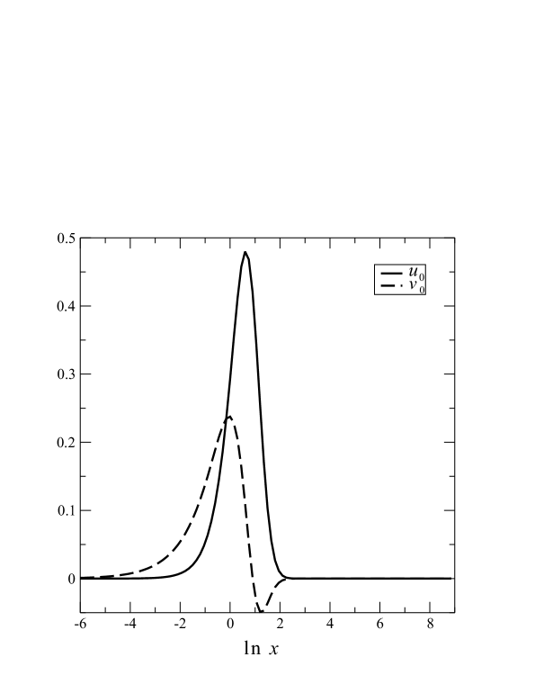
Рис. 1: Solutions of the Dirac equation for SLE

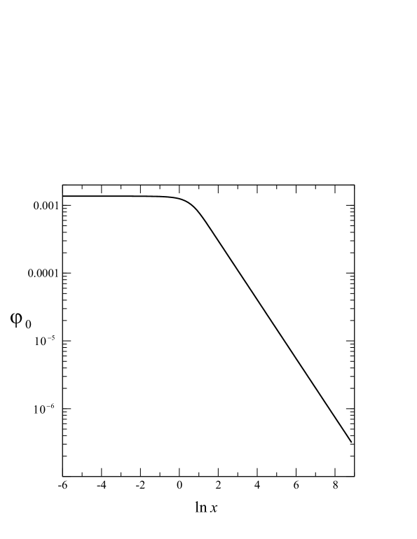
Рис. 2: Self-consistent potential of SLE

The equations (49) and (II) lead to the following relation between the "bare"charge $e_{0}$ and the integral charge of SLE:

$$e_{0}\frac{(1-C)}{(1+C)}=e;$$

$$e\ e_{0}=4\pi a,\quad e=\frac{4\pi a}{e_{0}}\approx-\frac{41.42}{e_{0}}.$$ (73)

It is of interest that the formula (III) has the same structure and consequences that result from the Dirac monopole theorymonopol despite of a different physical interpretation. In particular, if the calculated self-localized one-particle excitation of the electron-positron field (EPF) could be considered as a "physical"electron the only possible value of the parameter $a_{0}$ together with the ratio (III) leads to the condition of the observed charge quantization with the fixed value of the "bare"charge $e_{0}$. Indeed, on the analogy with the "polaron"theory bipolaron ,Solodovnikova1 n-particle excitation of EPF can be considered as the superposition of n different SLE’ that are at the distances exceeding the size of localization $\Delta r$. Then the charge of such n-soliton excitation $q_{n}$ would be always multiple to the elementary charge of SLE $q_{n}=ne$.

IV EPF quasi-particle excitation with an arbitrary momentum

In the previous section we have considered the possibility for a resting quasi-particle with a non-trivial self-consistent charge distribution, the finite energy $E(0)$ and a zero total momentum $\vec{P}=0$ to exist in the framework of a nonperturbative QED.

The obtained solution allows one to imagine the internal structure of the resting "physical"electron (positron) as a strongly coupled state of charge distributions of the opposite sign, the large values of integral charges of these distributions compensating each other almost completely and their heavy masses being "absorbed"by the binding energy.

Actually the energy $\pm E(0)$ defines the boundaries of the renormalized electron and positron zones resulting from the strong polarization of EPF when the excitation appears. But this excitation could be interpreted as the "physical"electron (positron) if the sequence of the levels in every zone determined by the vector $\vec{P}\not=0$ (Fig.1) were described by the relativistic energy spectrum of real particles, that is

$$E(\vec{P})=\sqrt{P^{2}+E^{2}(0)}=\sqrt{P^{2}+m^{2}}.$$ (74)

Only in this case the energy E(0) can really be used for calculating the mass $m_{0}$ of the "bare"electron.

It is worth saying, that the problem of studying the dynamics of the self-localized excitation should be solved for any system with a strong interaction between quantum fields in order to calculate its effective mass. For example, a similar problem for Pekar "polaron"Pekar in the ionic crystal was considered in papers PV ,Bogol , Tyablikov , Feynmanpol , Gross and in many more recent works. It is essential that because of the non-linear coupling between the particle and a self-consistent field the energy dispersion $E(\vec{P})$ for the quasi-particle proves to be very complicated. As the result, its dynamics in the crystal is similar to the motion of the point "physical"particle only at a small enough total momentum.

However, in the case of QED the problem is formulated in a fundamentally different way. There is currently no doubt that the dynamics of the "physical"excitation should be described by the formula (74) for any (!) values of the momentum $\vec{P}$. It means that the considered nonperturbative approach for describing the internal structure of the "physical"electron should lead to the energy dispersion law (74) for the entire range of the momentum $\vec{P}$.

The rigorous method of taking into account the translational symmetry in the strong coupling theory for the "polaron"problem was elaborated in the works of Bogolubov Bogol and Gross Gross . Let’s remember that this method was based on the introduction of the collective variable $\vec{R}$ conjugated to the total momentum operator $\hat{\vec{P}}$, the canonical character of the transformation caused by three new variables $R_{i}$ being provided by the same number of additional conditions imposed on the other variables of the system. In the "polaron"problem the quantum field interacting with the particle contributes to the total momentum of the system. It allows one to impose these conditions on the canonical field variables Bogol , Gross and the concrete form of the variable transformation is based mainly on the permutation relations for the boson field operators.

The considered problem has some specific features in comparison with the "polaron"problem. Firstly, the formation of the one-particle wave packet is the multi-particle effect because this packet includes all initial states of EPF as the fermionic field. Secondly, its self-localization is provided by the polarization potential of the scalar field that doesn’t contribute to the total momentum of the system. Therefore, we use a different approach in order to select the collective coordinate $\vec{R}$. Let us return to the configuration representation in the Hamiltonian (II) , where QED is considered to be the totality of N $(N\rightarrow\infty)$ point electrons interacting with the quantum EMF in the Coulomb gauge Heitler :

$$\hat{H}=\sum_{a=1}^{N}\{\vec{\alpha}_{a}[\hat{\vec{p}_{a}}+e_{0}\hat{\vec{A}}(\vec{r}_{a})]+\beta_{a}m_{0}+e_{0}\hat{\varphi}(\vec{r}_{a})\}-$$

$$\frac{1}{2}\int d\vec{r}(\vec{\nabla}\hat{\varphi}(\vec{r}))^{2}+\sum_{\vec{k}\lambda}\omega(\vec{k})\hat{n}_{\vec{k}\lambda};$$

$$\omega(\vec{k})=k;\quad\hat{n}_{\vec{k}\lambda}=c^{+}_{\vec{k}\lambda}c_{\vec{k}\lambda};\quad\lambda=1,2;$$

$$\hat{\vec{A}}(\vec{r})=\sum_{\vec{k}\lambda}\frac{1}{\sqrt{2k\Omega}}\vec{e}^{(\lambda)}[c_{\vec{k}\lambda}e^{i\vec{k}\vec{r}}+c^{+}_{\vec{k}\lambda}e^{-i\vec{k}\vec{r}}]$$ (75)

Here $\Omega$ is the normalized volume; $c^{+}_{\vec{k}\lambda}(c_{\vec{k}\lambda})$ are the operators of the creation (annihilation) of quanta of a transversal electromagnetic field, the quantum having the wave vector $\vec{k}$, polarization $\vec{e}^{(\lambda)}$ and energy $\omega(\vec{k})=k$. The sign of the interaction operators differs from the standard one because the parameter $e_{0}$ is introduced as a positive quantity.

As it was stated above the zero approximation of nonperturbative QED is defined only by a strong interaction of electrons with the scalar field, where the interaction with the transversal field is to be taken into account in the framework of the standard perturbation theory when the conservation of the total momentum is provided automatically Akhiezer . Therefore, while describing the quasi-particle excitation we should consider the conservation of the total momentum only for the system of electrons. In the considered representation it is defined by the sum of the momentum operators of individual particles

$$\hat{\vec{P}}=\sum_{a=1}^{N}\hat{\vec{p}_{a}};$$

$$\hat{\vec{P}}|\Phi_{1}(\vec{P})>=\vec{P}|\Phi_{1}(\vec{P})>.$$ (76)

It means that in the configuration space the variable $\vec{R}$ conjugated to the total momentum is simply a coordinate of the center of mass and the desired transformation to new variables is as follows:

$$\vec{r}_{a}=\vec{R}+\vec{\rho}_{a};\quad\vec{R}=\frac{1}{N}\sum_{a=1}^{N}\vec{r}_{a};\quad\sum_{a=1}^{N}\vec{\rho}_{a}=0;$$

$$\hat{\vec{p}_{a}}=-i\vec{\nabla}_{a}=-\frac{i}{N}\vec{\nabla}_{R}+\hat{\vec{p}^{\prime}_{a}};\quad\hat{\vec{P}}=-i\vec{\nabla}_{R};\quad\hat{\vec{p}^{\prime}_{a}}=-i\vec{\nabla}_{\rho_{a}}+\frac{i}{N}\sum_{b=1}^{N}\vec{\nabla}_{\rho_{b}};\quad\sum_{a=1}^{N}\hat{\vec{p}^{\prime}_{a}}=0.$$ (77)

The Hamiltonian (IV) with new variables is of the following form

$$\hat{H}=\sum_{a=1}^{N}\{\vec{\alpha}_{a}[-\frac{i}{N}\vec{\nabla}_{R}+\hat{\vec{p}^{\prime}_{a}}+e_{0}\hat{\vec{A}}(\vec{\rho}_{a}+\vec{R})]+\beta_{a}m_{0}+e_{0}\hat{\varphi}(\vec{\rho}_{a}+\vec{R})\}-$$

$$\frac{1}{2}\int d\vec{r}(\vec{\nabla}\hat{\varphi}(\vec{r}))^{2}+\sum_{\vec{k}\lambda}\omega(\vec{k})\hat{n}_{\vec{k}\lambda}.$$ (78)

It should be noted that the matrix elements of an arbitrary operator in a new configuration representation are to be calculated in accordance with the following norm (we introduce a special notation for this norm)

$$<<\Phi_{1}|\hat{M}|\Phi_{2}>>=\int d\vec{R}\prod_{a}d\vec{\rho}_{a}\Phi_{1}^{*}(\vec{R},\{\vec{\rho}_{a}\})\hat{M}\Phi_{2}(\vec{R},\{\vec{\rho}_{a}\}).$$ (79)

Let us denote by $\hat{H}_{0}$ that part of the operator (IV) which doesn’t depend on the transversal EMF and describes the internal structure of "physical"particles. In fact, the operator $\hat{H}_{0}$ doesn’t depend on the coordinate $\vec{R}$ either, because of its commutativity with the operator of the total momentum of the system of electrons. This also follows from the well known result Heitler that in the Coulomb gauge the scalar potential could be excluded from the hamiltonian. As a result the operator $\hat{H}_{0}$ depends only on the vector differences $(\vec{r}_{a}-\vec{r}_{b})=(\vec{\rho}_{a}-\vec{\rho}_{b})$ and doesn’t change with the simultaneous translation of all the coordinates. As a consequence, the eigenfunctions of the hamiltonian $\hat{H}_{0}$ depend on the coordinate $\vec{R}$ in the same way as for a free particle:

$$\Phi(\vec{R},\{\vec{\rho}_{a}\})=\frac{1}{(2\pi)^{3/2}}e^{i\vec{P}\vec{R}}|\Phi_{1}(\vec{P},\{\vec{\rho}_{a}\})>;$$

$$\hat{H}_{0}\rightarrow\hat{H}_{0}(\vec{P})=\sum_{a=1}^{N}\{\vec{\alpha}_{a}[\frac{1}{N}\vec{P}+\hat{\vec{p}^{\prime}_{a}}]+\beta_{a}m_{0}+e_{0}\hat{\varphi}(\vec{\rho}_{a})\}-\frac{1}{2}\int d\vec{r}(\vec{\nabla}\hat{\varphi}(\vec{r}))^{2}$$ (80)

Further calculations consist in returning to the field representation by the variables $\vec{\rho}_{a}$ in the limit $(N\rightarrow\infty)$ and in using the approximate trial wave packet $|\Phi_{1}(\vec{P})>$ similar to (II) but with the coefficient functions depending on $\vec{P}$ . Thus, in the framework of non-perturbation QED the orthogonalized and normalized set of states for the EPF one-particle excitation is defined as follows

$$|\Phi^{(0)}_{1}(\vec{P})>\simeq\frac{1}{(2\pi)^{3/2}}e^{i\vec{P}\vec{R}}\int d\vec{q}\{U_{\vec{q}s}(\vec{P})a^{+}_{\vec{q}s}+V_{\vec{q}s}(\vec{P})b^{+}_{\vec{q}s}\}|0;0;\varphi(\vec{r})>;$$ (81)

with the norm (79) and the coefficient functions $U_{\vec{q}s}(\vec{P});V_{\vec{q}s}(\vec{P})$.

Using the coordinate representation for these functions

$$\Psi_{\nu}(\vec{r},\vec{P})=\int\frac{d\vec{q}}{(2\pi)^{3/2}}\sum_{s}U_{\vec{q}s}(\vec{P})u_{\vec{q}s\nu}e^{i\vec{q}\vec{r}};$$

$$\Psi^{c}_{\nu}(\vec{r},\vec{P})=\int\frac{d\vec{q}}{(2\pi)^{3/2}}\sum_{s}V_{\vec{q}s}(\vec{P})v_{\vec{q}s\nu}e^{i\vec{q}\vec{r}},$$ (82)

one can find the following functional for calculating the value $E(\vec{P})=E_{1}^{(0)}-E_{0}^{(0)}$ corresponding to the energy of one-particle excitation with an arbitrary momentum

$$E(\vec{P})=\int d\vec{r}\{\Psi^{+}(\vec{r},\vec{P})[(\vec{\alpha}\vec{P}-i\vec{\alpha}\vec{\nabla}+\beta m_{0})+e_{0}\frac{1}{2}\varphi(\vec{r},\vec{P})]\Psi(\vec{r},\vec{P})-$$

$$\Psi^{+c}(\vec{r},\vec{P})[(-\vec{\alpha}\vec{P}-i\vec{\alpha}\vec{\nabla}+\beta m_{0})+e_{0}\frac{1}{2}\varphi(\vec{r},\vec{P})]\Psi^{c}(\vec{r},\vec{P});$$

$$\varphi(\vec{r},\vec{P})=e_{0}\int\frac{d\vec{r}^{\prime}}{|\vec{r}-\vec{r}^{\prime}|}[\Psi^{+}(\vec{r}^{\prime},\vec{P})\Psi(\vec{r}^{\prime},\vec{P})-\Psi^{+c}(\vec{r}^{\prime},\vec{P})\Psi^{c}(\vec{r}^{\prime},\vec{P})];$$

$$\int{d\vec{r}}[\Psi^{+}(\vec{r},\vec{P})\Psi(\vec{r},\vec{P})+\Psi^{+c}(\vec{r}^{\prime},\vec{P})\Psi^{c}(\vec{r}^{\prime},\vec{P})]=1.$$ (83)

It should be noted that the mean value of the operator $\hat{H}_{0}(\vec{P})$ in the representation of the second quantization was calculated by taking into account the expression

$$\lim_{N\to\infty}\frac{1}{N}\sum_{\vec{p}}=1,$$

that follows from a well known formula for the density of states when EPF is quantized within the normalized volume $\Omega$ Akhiezer .

It was mentioned above, that there is quite a close analogy between the nonperturbative description of QED and the theory of strong coupling in the "polaron"problem. Therefore, it is of interest to compare the obtained functional (IV)with the results of various methods of including the translational motion in the "polaron"problem. The simplest one was used by Landau and Pekar PV who introduced the Lagrange multipliers in the form

$$J(\vec{P})=J(\vec{P}=0)+(\vec{P}\vec{V}),$$ (84)

with the functional $J(\vec{P}=0)$ referring to a resting "polaron"and the Lagrange multiplier $V_{i}$ denoting the components of the quasi-particle average velocity.

We can see that the obtained functional(IV) has the same form as (84)if the relativistic velocity of the excitation is determined by the formula

$$\vec{V}=\int d\vec{r}\{\Psi^{+}(\vec{r},\vec{P})(\vec{\alpha})\Psi(\vec{r},\vec{P})+\Psi^{+c}(\vec{r},\vec{P})(\vec{\alpha})\Psi^{c}(\vec{r},\vec{P})\}.$$ (85)

This corresponds to the well known interpretation of Dirac matrixes.

Varying this functional by taking into account the normalized conditions leads to the following equations for the wave functions

$$\{(\vec{\alpha}\vec{P}-i\vec{\alpha}\vec{\nabla}+\beta m_{0})+e_{0}\varphi(\vec{r},\vec{P})-E(\vec{P})\}\Psi(\vec{r},\vec{P})=0;$$

$$\{(\vec{\alpha}\vec{P}+i\vec{\alpha}\vec{\nabla}-\beta m_{0})-e_{0}\varphi(\vec{r},\vec{P})-E(\vec{P})\}\Psi^{c}(\vec{r},\vec{P})=0.$$ (86)

These equations show that unlike the "polaron"problem Bogol , the translational motion of the quasi-particle determining the momentum $\vec{P}$ is related in our case to its internal movement described by the coordinate $\vec{r}$ by means of spinor variables only. The physical reason for this separation of variables is explained by the fact that in QED the self-localized state is formed by the scalar field, and its interaction with the particle doesn’t involve the momentum exchange. In order to find the analytical energy spectrum $E(\vec{P})$ the system of non-linear equations(IV should be diagonalized relative to the spinor variables. The possibility of such diagonalization seems to be a non-trivial requirement for the nonperturbative QED under consideration.

The solution of the equations (IV) can be found on the basis of the states for which the dependence on the vector $\vec{q}$ in the wave packet amplitudes $U_{\vec{q},s},V_{\vec{q},s}$ remains the same as it was in the motionless "physical"electron. However, the relation between the spinor components of these functions can be changed. But as the self-consistent scalar potential involves the summation over all spinor components it can be assumed that the potential doesn’t depend on the momentum for the class of states in question:

$$\varphi(\vec{r},\vec{P})=\varphi(r)|_{\vec{P}=0}.$$ (87)

In the coordinate representation the transformation of the spinor components of the wave functions satisfying the equations (IV) takes place because of the dependence on the momentum. It seems that there are some general arguments based on the Hamiltonian symmetry that make the diagonalization of equations (IV) easier. However, we have desired the solution by sorting out various linear combinations of the wave functions found in Section 3 for a resting electron. These functions correspond to the degenerated states in the case of $\vec{P}=0$ but are mixed for a moving electron. It is found that there is only one normalized linear combination satisfying all the necessary conditions of self-consistency :

$$\Psi(\vec{r},\vec{P})=L(\vec{P})\Psi(\vec{r})+K(\vec{P})\tilde{\Psi^{c}}(\vec{r});$$

$$\Psi^{c}(\vec{r},\vec{P})=L_{1}(\vec{P})\Psi^{c}(\vec{r})+K_{1}(\vec{P})\tilde{\Psi}(\vec{r});$$

$$|L|^{2}+|K|^{2}=|L_{1}|^{2}+|K_{1}|^{2}=1.$$ (88)

The condition (87) according to which the potential doesn’t depend on the momentum for the excitation at the energy $E(\vec{P})$, is fulfilled if the coefficients are related as

$$L_{1}=-K;\qquad K_{1}=L.$$ (89)

These relations are also consistent with Equations (IV) for wave functions.

This means that the "physical"electron moves in such a way that its states are transformed in the phase space of the orthogonal wave functions (26),(35),(44),(49)but the amplitudes of its "internal"charge distributions are not changed. These results, however, are valid only for the case of neglecting the interaction with the transverse electromagnetic field.

Substituting the superpositions (IV) into equations (IV) we use the following relations:

$$(\vec{\alpha}\vec{P})\Psi(\vec{r})=\left(\begin{array}[]{c}if(r)(\vec{\sigma}\vec{P})\Omega_{1/2,1,M}\\ g(r)(\vec{\sigma}\vec{P})\Omega_{1/2,0,M}\end{array}\right);\quad(\vec{\alpha}\vec{P})\Psi^{c}(\vec{r})=\left(\begin{array}[]{c}g_{1}(r)(\vec{\sigma}\vec{P})\Omega_{1/2,1,M}\\ -if_{1}(r)(\vec{\sigma}\vec{P})\Omega_{1/2,0,M}\end{array}\right);$$ (94)

$$(-i\vec{\alpha}\vec{\nabla}+\beta m_{0}+e_{0}\varphi)\Psi(\vec{r})=E(0)\left(\begin{array}[]{c}g(r)\Omega_{1/2,0,M}\\ if(r)\Omega_{1/2,1,M}\end{array}\right);$$ (97)

$$(-i\vec{\alpha}\vec{\nabla}+\beta m_{0}+e_{0}\varphi)\Psi^{c}(\vec{r})=-E(0)\left(\begin{array}[]{c}-if_{1}(r)\Omega_{1/2,0,M}\\ g_{1}(r)\Omega_{1/2,1,M}\end{array}\right),$$ (100)

and similar formulas for the functions $\tilde{\Psi}(\vec{r});\tilde{\Psi^{c}}(\vec{r})$; $\sigma_{i}$ are the Pauli matrixes.

For equations (IV) to be fulfilled for any vector $\vec{r}$ it is necessary to set the coefficients of spherical spinors equal to the same indexes $l$. The corresponding radial functions are proved to be the same under these conditions, and the following system of equations for the spinors $\chi_{0,1}^{\pm}$ is obtained

$$iL(\vec{\sigma}\vec{P})\chi^{+}_{1}+K(E+E_{0})\chi_{1}^{+}=0;\quad iK(\vec{\sigma}\vec{P})\chi^{+}_{0}+L(E-E_{0})\chi_{0}^{+}=0;$$

$$L(\vec{\sigma}\vec{P})\chi^{+}_{0}+iK(E+E_{0})\chi_{0}^{+}=0;\quad K(\vec{\sigma}\vec{P})\chi^{+}_{1}+iL(E-E_{0})\chi_{1}^{+}=0;$$

$$L_{1}(\vec{\sigma}\vec{P})\chi^{-}_{1}-iK_{1}(E-E_{0})\chi_{1}^{-}=0;\quad K_{1}(\vec{\sigma}\vec{P})\chi^{-}_{0}-iL_{1}(E+E_{0})\chi_{0}^{-}=0;$$

$$iL_{1}(\vec{\sigma}\vec{P})\chi^{-}_{1}-K_{1}(E-E_{0})\chi_{1}^{-}=0;\quad iK_{1}(\vec{\sigma}\vec{P})\chi^{-}_{0}-L_{1}(E+E_{0})\chi_{0}^{-}=0.$$ (101)

Spin variables in Equations (IV) are also separated. In order to show this one can use, for example, the relation between the coefficients resulting from the 4th equation in (IV) in the first one of these equations:

$$\chi_{1}^{+}=i\frac{K(\vec{\sigma}\vec{P})\chi^{+}_{1}}{L(E-E_{0})}.$$

As aresult there exists a non-trivial solution of these equations for two branches of the energy spectrum

$$E_{e,p}=\pm\sqrt{E^{2}_{0}+P^{2}},$$ (102)

referring to the electron and positron zones, respectively (Fig.1). The same expressions can be obtained for all conjugated pairs of the equations in (IV). The coefficients in the wave functions (IV) can be found taking into consideration the normalization condition:

$$L^{e}=K^{e}_{1}=\frac{P}{\sqrt{P^{2}+(E_{e}-E_{0})^{2}}};\quad K^{e}=-L^{e}_{1}=\frac{E_{e}-E_{0}}{\sqrt{P^{2}+(E_{e}-E_{0})^{2}}};$$

$$L^{p}=K^{p}_{1}=\frac{P}{\sqrt{P^{2}+(E_{e}+E_{0})^{2}}};\quad K^{p}=-L^{p}_{1}=-\frac{E_{e}+E_{0}}{\sqrt{P^{2}+(E_{e}+E_{0})^{2}}}.$$ (103)

One can see that this set of coefficients coincides with the set of spinor components for solving the Dirac equation for a free electron with the observed mass $m=E_{0}$. Thus, the results of this section show that the "internal"structure of the "physical"electron (positron) considered in this paper is consistent with the experimental energy dispersion (102) for a real free particle due to the relativistic invariance of the Dirac equation.

For the interpretation of the wave packet (81) as the state vector for a "physical"particle it is essential that it is the eigenvector of the total momentum of EPF in the framework of the considered "quenched QED". It means that SLE with different momenta form the set of orthogonal and normalized functions if the condition (79) is taken into account:

$$<<\Phi^{(0)}_{1}(\vec{P}_{1})|\Phi^{(0)}_{1}(\vec{P})>>=\delta(\vec{P}-\vec{P}_{1}).$$ (104)

V Conclusions

Thus, in the present paper new variational self-consistent equations for interacting electron-positron and scalar electromagnetic fields have been derived in the framework of the "large-$\alpha$ QED". These equations differ from the Schwinger-Dyson equations and describe the one-particle excitation of the system that doesn’t contain the quanta of the transversal electromagnetic field.

The soliton-like solution of the desired equations has been calculated numerically. It includes a non-zero integral charge ("charge"soliton) and can be regarded as the spatially localized collective excitation of the electron-positron field coupled with the localized scalar field. It is shown that this solution is unique if the coupling constant $\alpha_{0}$ for the field interaction is fixed. This result leads to the quantization condition for the "observed"charge of $n$-soliton excitations of the system.

The dependence of the energy of the soliton-like excitation on its total momentum has been also studied. It is shown that the corresponding law of the energy dispersion is consistent with Lorentz invariance of QED and the effective mass of the "charge soliton"can be calculated.

It should be emphasized that the main aim of the paper is to prove the possibility of the existence of such non-trivial solutions of the "large-$\alpha$ QED"equations that could not be derived on the basis of the standard perturbation theory. However, the physical interpretation of the desired solution requires further research.

- (1) J.R.Hiller and S.J.Brodsky, Phys. Rev. D, 59,(1998), 016006.
- (2) Proceedings: Fluctuating Paths and Fields, (Singapore, World Scientific, 2001).
- (3) S.P.Klevansky, Rev. of Modern Phys, 64,(1992), 649.
- (4) J.Schwinger, Phys. Rev. , 125,(1962),397; R.Fukuda and R.Kugo, Nucl. Phys. , B117,(1976),250;P.I.Fomin, V.P.Gusynin, V.A.Miransky and Y.A.Sytenko, Riv. Nuovo Chim. , 6,(1983),1.
- (5) Y.Kikichi and Y.Ng, Phys.Rev. D , 38,(1988),3578; V.P.Gusynin, V.A.Miransky and I.A.Shovkovy, Phys.Rev. D , 67,(2003),107703.
- (6) P.M.Morse and H.Feshbach, Methods of Theoretical Physics, (N.Y.:McGraw-Hill Book Co., 1953).
- (7) H.Fröhlich , Adv. Phys. , 3,(1954),325.
- (8) C.Alexandrou, R.Rosenfelder and A.W.Schreiber , Phys.Rev. D , 62,(2000),085009.
- (9) R.P.Feynman, Phys. Rev., 97,(1955), 660.
- (10) S.I.Pekar, Zh. Exper. Teor. Fiz., 16,(1946), 769-774.
- (11) N.N.Bogoliubov, Uspekhi Matematicheskih Nauk, 2,(1950), 3-24.
- (12) S.V.Tyablikov, Zh. Exper. Teor. Fiz., 21,(1951), 377-388.
- (13) D.Pines, Polarons and Excitons, G.G.Kuper, G.D.Whitfield, eds., (N.Y.:Plenum Press, 1962, p. 155).
- (14) Polarons. Ed. Yu.B.Firsov, (Moscow: Nauka, 1973).
- (15) I.D.Feranchuk, arXiv: hep-th/0309072.
- (16) Gross E.P. Annals of Physics (NY), 99,(1976), 1.
- (17) G.Hainzl, M.Lewin and E.Sere , J. of Phys. A, 38,(2005), 4483.
- (18) I.D.Feranchuk, L.I.Komarov and A.P.Ulyanenkov, Ann. Phys. (N.Y.), 238,(1995), 370-440; J. of Phys. A, 29,(1996), 4035-4047; I.D.Feranchuk and A.A.Ivanov, J. of Phys. A, 37,(2004), 9841-9860.
- (19) L.I.Komarov, E.V.Krylov and I.D.Feranchuk, Zh. Numerical Math. and Math. Fiz., 18,(1978), 681-691; Zh. Teoret. and Math. Fiz., 32,(1977), 262.
- (20) Ya. M. Shnir Monopole, (Berlin, Springer, 2005).
- (21) E.M.Lifshitz and L.P.Pitaevskii, Relativistic Quantum Theory. Part II, (Moscow, Nauka, 1971).
- (22) N.N.Bogoliubov, Quasi-mean Values in The Problems of Statistical Mechanics. In "Selected Works v.3, (Kiev, "Navukova Dumka 1971).
- (23) W.Heitler, The Quantum Theory of Radiation, (Oxford, The Clarendon Press, 1954).
- (24) L.D.Landau and E.M.Lifshitz Quantum Mechanics, (Moscow, Nauka, 1963).
- (25) A.I.Akhiezer and V.B.Beresteckii, Quantum Electrodynamics, (Moscow, Nauka, 1969).
- (26) V.I.Yukalov, Vestnik Moscow Univ.(russian) 23,(1976), 10; Teoret. Matem. Fiz.(russian) 28,(1976), 652.
- (27) W.E.Caswell, Ann. Phys. (N.Y.), 123,(1979), 153.
- (28) I.D.Feranchuk and L.I.Komarov, Phys. Lett. A, 88,(1982), 211-213.
- (29) E.S.Fradkin, Proceedings of Fiz. Inst. of Soviet Academy of Science, 29,(1965), 1-154; Nucl. Phys. 76, (1966), 588.
- (30) E.P.Zhidkov, G.I.Makarenko and I.V.Puzynin, Elementary Particles and Atomic Nuclei, Dubna, JINR , 4,(1973), 127-166.
- (31) S.K.Godunov and V.S.Ryabenkii Introduction to the theory of finite-difference schemes (Moscow, Fizmatgiz, 1962).
- (32) V.L.Vinetzkii,Zh.of Exper. and Theoret. Physics,40,(1961), 1459.
- (33) E.P.Solodovnikova and A.N.Tavhelidze,Teoret. and Math. Fiz.,21,(1974), 13.
- (34) L.D.Landau and S.I.Pekar,Zh.of Exper. and Theoret. Physics,18,(1948), 419.
- (35) G. Hö ler,Zh. Phyzik,146,(1956), 372.
- (36) E.P.Solodovnikova, A.N.Tavhelidze and O.A.Khrustalov,Teoret. and Math. Fiz., 11,(1972), 317.
- (37) S.T.Zavtrak, L.I.Komarov and I.D.Feranchuk,Teoret. and Math. Fiz.,47,(1981), 55.