A class of nonholonomic kinematic constraints in elasticity

Abstract

We propose a first example of a simple classical field theory with nonholonomic constraints. Our model is a straightforward modification of a Cosserat rod. Based on a mechanical analogy, we argue that the constraint forces should be modeled in a special way, and we show how such a procedure can be naturally implemented in the framework of geometric field theory. Finally, we derive the equations of motion and we propose a geometric integration scheme for the dynamics of a simplified model.

1 Introduction

Motivation

Nonholonomic constraints in mechanical systems have a long and illustrious history going back to the work of Hertz at the end of the nineteenth century. For nonholonomic constraints in field theories, the case is not so clear, and to the best of our knowledge, no convincing example has been proposed to this day. In this paper, we intend to rectify this omission by giving a simple example of a continuum theory with nonholonomic constraints. The basic model is that of a Cosserat rod, a special kind of continuum theory. This rod moves in a horizontal plane which is supposed to be sufficiently rough, so that the rod rolls without sliding.

In the Cosserat theory one assumes that the laminae at right angles to the centerline are rigid discs. The nonholonomic Cosserat rod therefore touches the plane along a curve (rather than in an open subset of the plane, which would be the case for a fully three-dimensional continuum) and the nonholonomic constraint translates to the fact that the instantaneous velocity of these contact points is zero.

Our example can also be modeled as the continuum limit of a nonholonomic mechanical system. Consider $N$ rigid discs rolling vertically without sliding on a horizontal plane, and assume that these discs are interconnected by flexible beams of length $\ell/N$, as in figure 1. Now let the number of discs go to infinity, while keeping the total length $\ell$ fixed: the result is the nonholonomic Cosserat rod.

This mechanical model is interesting for a number of reasons. First of all, the nonholonomic field equations are derived by varying the action with respect to admissible variations, and this obviously requires the specification of a bundle of admissible variations, or equivalently, a bundle of reaction forces. In mechanics, this is commonly done by taking recourse to the principle of d’Alembert, which states that the virtual work of the reaction forces is zero. In field theory, this principle can be interpreted in a number of non-equivalent ways, and it is the mechanical model which will eventually determine our choice.

Secondly, our model is a counterexample to the often-held belief that constraints in classical field theories are necessarily vakonomic. In sections 1.1 and 1.2 these two aspects are treated more in detail.

Plan of the paper

After giving a quick overview of jet bundle theory, we derive the Euler-Lagrange equations in the presence of nonholonomic constraints. Our treatment relies on the fact that the space of independent variables is a product of space and time, and that the fields are sections of a trivial fibre bundle. This is the case, for instance, for nonrelativistic elasticity. These assumptions allow us to split the jet bundle in a part involving spatial derivatives, and a part involving derivatives with respect to time. Using this natural splitting, we propose a bundle of reaction forces, based on the mechanical model (to be outlined in section 1.2). As we shall see, these reaction forces are very similar to the ones used in mechanics.

The remainder of the paper is then devoted to the study of a specific example of a nonholonomic field theory. First, we give an outline of the theory of Cosserat rods moving in the plane, and we pay particular attention to aspects of symmetry. In the second part, we then outline a suitable class of nonholonomic constraints, and we derive the equations of motion. The paper concludes with a brief foray into the field of geometric integration, where a simple explicit algorithm for the integration of the nonholonomic dynamics is proposed.

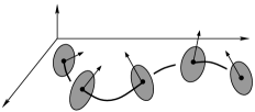
Figure 1: Geometry of the constrained rod

1.1 Relation with other approaches

In a number of papers [1, 2], Bibbona, Fatibene, and Francaviglia contrasted the vakonomic and the nonholonomic treatments for classical field theories, and showed that for relativistic hydrodynamics only the former gives correct results. Another typical example of a vakonomic constraint is the incompressibility constraint in nonrelativistic fluid dynamics, treated by Marsden et al. [3]. Many more can be found in Antman’s book [4] and in the papers by García et al. [5].

In contrast, our field theory arises as the continuum limit of the vertically rolling disc, a textbook example of a nonholonomic mechanical system. These nonholonomic constraints survive in the continuum limit and hence provide a very strong motivation for the study of nonholonomic techniques in field theories.

In previous papers (see [6, 7, 8, 9]) various theoretical frameworks were established for the study of nonholonomic field theories. Our model fits into these descriptions, but involves a number of additional ingredients which cannot be derived from these theoretic considerations alone. In particular the bundle of reaction forces takes a special form, motivated by similar definitions from mechanics.

It should also be noted that similar theories as ours were explored before by Vignolo and Bruno (see [10]). They considered constraints depending only on the time derivatives of the fields, and their resulting analysis is therefore more direct. However, the underlying philosophy is the same: the constraints are “(…) purely kinetic restrictions imposed separately on each point of the continuum”.

1.2 Modeling the constraint forces

Nonholonomic mechanical systems

The mechanical background is not essential for the description of the continuum theory, but rather serves as a justification for some of our definitions. In particular, it provides a number of valuable clues regarding the type of constraint forces needed to maintain such a nonholonomic constraint. Let $S$ be the configuration space of the vertically rolling disc, so that the configuration space for the entire model, consisting of $N$ discs, is the product space $S^{N}$. Denote by $\varphi^{\alpha}_{(i)}$ the constraints of rolling without sliding imposed on the $i$th wheel; $\varphi^{\alpha}_{(i)}$ is a function on $TS^{N}$.

With these conventions, a motion of the system is a curve $t\mapsto c(t)$ in $S^{N}$, and a variation of such a motion $c$ is then a vector field $(X_{1},X_{2},\ldots,X_{N})$ on $S^{N}$ along $c$, i.e. a collection of maps $X_{i}:\mathbb{R}\rightarrow TS$ such that $X_{i}(t)\in T_{c^{i}(t)}S$ for all $i=1,\ldots,N$, where $c^{i}:=\mathrm{pr}_{i}\circ c$.

Let us now consider the one-forms $\Phi_{(i)}^{\alpha}:=J^{\ast}(\mathrm{d}\varphi_{(i)}^{\alpha})$, where $J$ is the vertical endomorphism on $TS^{N}$. In geometric mechanics, linear combinations of these one-forms represent the possible reaction forces at the $i$th wheel; the bundle $F$, defined as

$$F:=\left<{\Phi^{\alpha}_{(1)}}\right>\oplus\left<{\Phi^{\alpha}_{(2)}}\right>\oplus\cdots\oplus\left<{\Phi^{\alpha}_{(N)}}\right>$$

then represents the totality of all reaction forces along the rod. In coordinates, the one-forms $\Phi^{\alpha}_{(i)}$ are given by

$$\Phi^{\alpha}_{(i)}=\frac{\partial\varphi^{\alpha}_{(i)}}{\partial\dot{y}_{(i)}}\mathrm{d}y_{(i)}\quad\left(=\sum_{a}\frac{\partial\varphi^{\alpha}_{(i)}}{\partial\dot{y}^{a}_{(i)}}\mathrm{d}y^{a}_{(i)}\right)\quad\mbox{for all}\>i=1,\ldots,N.$$ (1)

Here, $(y_{(i)},\dot{y}_{(i)})$ is a coordinate system on the $i$th factor of $TS^{N}$. Note that there is no summation over the index $i$ in (1), and that the summation over individual coordinates is implicit, as shown in the term between brackets.

Knowing the precise form of the bundle of reaction forces $F$ is important because the nonholonomic equations of motion are derived by varying the action with respect to admissible variations. Moreover, the principle of d’Alembert shows us that a variation is admissible if it belongs to the annihilator of $F$, i.e. a variation $(X_{1},\ldots,X_{N})$ of $c$ is admissible if

$$\left<\bar{X}_{i}(t),\alpha(c(t))\right>=0,\quad\mbox{for all}\>(i,t)\in\{1,\ldots,N\}\times\mathbb{R}\quad\mathrm{and}\quad\alpha\in F,$$ (2)

where $\bar{X}_{i}$ is a lift of $X_{i}$ to $T(TS)$ such that $T\tau_{S}\circ\bar{X}_{i}=X_{i}$. Note that there is again no summation over $i$. In coordinates, this is equivalent to

$$v_{i}\frac{\partial\varphi_{(i)}}{\partial\dot{y}_{(i)}}\quad\mbox{for all}\>i=1,\ldots,N,$$ (3)

where we have written $X_{i}=v_{i}\frac{\partial}{\partial y_{(i)}}$.

In the next paragraph, we will let the number $N$ go to infinity, while keeping the length $\ell$ constant. The result is a field theory, and a reaction force will be a continuous assignment of a one-form on $TS$ to each point of the centerline of the rod. This definition will be the starting point for our treatment in the main body of the text; once we know the bundle of reaction forces, we can then derive the nonholonomic field equations.

The continuum model

In the continuum limit, a field is a map $\phi$ from $[0,\ell]\times\mathbb{R}$ to $S$. It is customary in classical field theory to view these fields as sections of a trivial bundle $\pi$, whose base space is $[0,\ell]\times\mathbb{R}$, and with standard fibre $S$. The role of the velocity space is then played by the first jet bundle $J^{1}\pi$, and the constraints $\varphi_{(i)}$ from the previous paragraph are replaced by a constraint function $\varphi^{\alpha}$ on $J^{1}\pi$.

In field theory, a variation of a field $\phi$ is now a map $X:[0,\ell]\times\mathbb{R}\rightarrow TS$ with the property that $X(s,t)\in T_{\phi(s,t)}S$; in other words, a vector field along $\phi$. Taking our cue from (3), we say that a variation $X$ is admissible if the following holds (in coordinates):

$$X(s,t)^{a}\frac{\partial\varphi^{\alpha}}{\partial y^{a}_{0}}=0,$$

where we have written $X(s,t)=X(s,t)^{a}\frac{\partial}{\partial y^{a}}$.

This condition can be rewritten in intrinsic form by using the following observation: as we shall show below, there exists a natural isomorphism between the first jet bundle and the product bundle $\mathbb{R}\times[J^{1}(M,S)\times_{S}TS]$. Now, let $J$ be the vertical endomorphism on $TS$. This map has a trivial extension to the whole of $\mathbb{R}\times[J^{1}(M,S)\times_{S}TS]$, and by using the natural isomorphism with $J^{1}\pi$, we obtain a map $J^{\ast}$ from $T^{\ast}(J^{1}\pi)$ to itself. The bundle $F$ of constraint forces is then generated by the forms $\Phi^{\alpha}:=J^{\ast}(\mathrm{d}\varphi^{\alpha})$. The similarity with the mechanical case is obvious.

2 Lagrangian field theories

In this paper, we will mostly be concerned with the description of elastic bodies. The geometric description of these theories is well known and we refer to [11, 12] for more information.

Let $M$ be a smooth $n$-dimensional compact manifold, and let $S$ be a general smooth $m$-dimensional manifold, with $n\leq m$. The points of $M$ are “material points”, labelling the points of the body, whereas $S$ is the physical space in which the body moves. In most cases, $S$ will be the Euclidian space $\mathbb{R}^{3}$, whereas $M$ can be one-, two-, or three-dimensional, corresponding to models of rods, shells, and three-dimensional continua. Furthermore, $M$ is assumed to be oriented, with volume form $\eta_{M}$.

On $M$ we consider a coordinate system $(x^{i})$ , $i=1,\ldots,n$, such that $\eta_{M}$ can locally be written as $\eta_{M}=\mathrm{d}x^{1}\wedge\cdots\wedge\mathrm{d}x^{n}$, and on $S$ we take a coordinate system $(y^{a})$, $a=1,\ldots,m$.

2.1 The bundle picture

In this section, we give a brief overview of the theory of jet bundles. For an introduction to classical field theory using jet bundles, we refer to [13, 14, 15] and the references therein.

Consider the fibre bundle $\pi:Y\rightarrow X$, where $X:=\mathbb{R}\times M$, $Y:=X\times S$, and the projection $\pi$ is the projection onto the first factor. The manifold $X$ is equipped with a coordinate system denoted by $(x^{\mu})$, where $\mu=0,\ldots,n$, and such that $x^{0}:=t$. Similarly, $S$ has a coordinate system $(x^{\mu},y^{a})$ which is adapted to the projection in the sense that the projection $\pi$ is locally given by $\mathrm{pr}_{2}:(x^{\mu},y^{a})\mapsto(x^{\mu})$. Note that $M$ is equipped with a volume form $\eta=\mathrm{d}t\wedge\eta_{M}$, which we write in coordinates as $\mathrm{d}^{n+1}x:=\mathrm{d}{x}^{0}\wedge\cdots\wedge\mathrm{d}{x}^{n}$. We will employ the following short-hand notation:

$$\mathrm{d}^{n}x_{\mu}:=\frac{\partial}{\partial x^{\mu}}\vrule height=0.0pt,depth=0.4pt,width=3.0pt\vrule height=7.0pt,depth=0.4pt\kern 3.0pt\eta=(-1)^{\mu}\mathrm{d}x_{0}\wedge\cdots\wedge\mathrm{d}x^{\mu-1}\wedge\mathrm{d}x^{\mu+1}\wedge\cdots\wedge\mathrm{d}x^{n}.$$

The first jet bundle $J^{1}\pi$ is the appropriate stage for Lagrangian first-order field theories. Its elements are equivalence classes of sections of $\pi$, where two sections are said to be equivalent at a point $x\in X$ if they have the same value at $x$ and if their first-order Taylor expansions at $x$ agree. The equivalence class of a section $\phi$ at $x$ is denoted by $j^{1}_{x}\phi$. Hence, $J^{1}\pi$ is naturally equipped with a projection $\pi_{1,0}:J^{1}\pi\rightarrow Y$, defined by $\pi_{1,0}(j^{1}_{x}\phi)=\phi(x)$, and a projection $\pi_{1}:J^{1}\pi\rightarrow X$, defined by $\pi_{1}(j^{1}_{x}\phi)=x$. The induced coordinate system on $J^{1}\pi$ is written as $(x^{\mu},y^{a};y^{a}_{\mu})$.

Furthermore, we define the manifold $J^{1}(M,S)$ of jets of mappings from $M$ to $S$ as the first jet manifold of the trivial bundle $\mathrm{pr}_{1}:M\times S\rightarrow M$. The usual jet bundle projections $\pi_{1}$ and $\pi_{1,0}$ induce projections $\pi_{M}$, onto $M$, and $\pi_{S}$, onto $S$, respectively.

Because of the special structure of the bundle $\pi$, viz. the fact that $X$ is the product $\mathbb{R}\times M$ and that $\pi$ is trivial, $J^{1}\pi$ can be written in a special form. Recall that the fibre coordinates of $J^{1}\pi$ represent the derivatives of the fields with respect to space and time: the decomposition of lemma 2.1 then provides an invariant way of making the distinction between time derivatives and spatial derivatives. Such an invariant decomposition is not possible for general jet bundles.

The bundle $\mathbb{R}\times[J^{1}(M,S)\times_{S}TS]$, a fibered product, consists of triples $(t,\kappa,v)$ such that $\pi_{S}(\kappa)=\tau(v)$, where $\tau:TS\rightarrow S$ is the tangent bundle projection. It is equipped with a projection $\hat{\pi}$ onto $Y$ defined as $\hat{\pi}(t,\kappa,v)=(t,\pi_{M}(\kappa);\tau(v))$. Moreover, $\hat{\pi}:\mathbb{R}\times[J^{1}(M,S)\times_{S}TS]\rightarrow Y$ is an affine bundle.

Lemma 2.1.

The first jet bundle $J^{1}\pi$ is isomorphic, as an affine bundle over $Y=\mathbb{R}\times M\times S$, to $\mathbb{R}\times[J^{1}(M,S)\times_{S}TS]$.

Proof:  A more general statement can be found in section 6B of [16].

Take any point $(t,m,s)$ in $\mathbb{R}\times M\times S$ and consider a $1$-jet $\gamma$ such that $\pi_{1,0}(\gamma)=(t,m,s)$. An alternative interpretation of $\gamma$ is that of a linear map $\gamma:T_{(t,m)}(\mathbb{R}\times M)\rightarrow T_{s}S$. Consider now the map $\Psi_{(t,m,s)}$, mapping $\gamma$ to the element of $\mathbb{R}\times[J^{1}(M,S)\times_{S}TS]$ given by

$$\Psi_{(t,m,s)}(\gamma)=\left(t,\gamma(0_{t},\cdot),\gamma\left(\frac{\partial}{\partial t}\Big{|}_{t},0_{m}\right)\right),$$

where $0_{m}$ and $0_{t}$ are the zero vectors in $T_{m}M$ and in $T_{t}\mathbb{R}$, respectively. It is easy to check that the map $\Psi$ is an isomorphism of affine bundles. $\Box$

In coordinates $(y^{a},\dot{y}^{a})$ on $TS$ and $(x^{i},y^{a};y^{a}_{;i})$ on $J^{1}(M,S)$, the isomorphism of lemma 2.1 is given by $(x^{\mu},y^{a};y^{a}_{\mu})\mapsto(t;x^{i},y^{a},y^{a}_{;i}=y^{a}_{i};y^{a},\dot{y}^{a}=y^{a}_{0})$.

For future reference, we remark here that the tangent bundle $TS$ is equipped with a $1$-$1$ tensor field, denoted by $J:T(TS)\rightarrow T(TS)$, and given in coordinates by

$$J=\frac{\partial}{\partial\dot{y}^{a}}\otimes\mathrm{d}y^{a}.$$

An intrinsic definition can be found in [17]. The adjoint of $J$ will be denoted by $J^{\ast}$ and is a map from $T^{\ast}(TS)$ to itself defined by $\left<{J^{\ast}(\alpha),v}\right>=\left<{\alpha,J(v)}\right>$, for all $v\in T(TS)$.

In section 3, we will encounter higher-order field theories, in particular of order $2$. In order to be able to deal with this type of field theory, we introduce the manifold $J^{k}\pi$ of $k$th order jets. The elements of $J^{k}\pi$ are again equivalence classes of sections of $\pi$, where two sections are equivalent at $x\in X$ if they have the same value at $x$ and if their Taylor expansions at $x$ agree up to the $k$th order. The $k$th order jet bundle is equipped with a number of projections $\pi_{k,l}:J^{k}\pi\rightarrow J^{l}\pi$ (where $l\leq k$), constructed by “truncating” to order $l$ the Taylor expansion defining an element of $J^{k}\pi$. A detailed account of jet bundles is provided in [18].

As a matter of fact, we will only need the third-order jet manifold $J^{3}\pi$. A natural coordinate system on $J^{3}\pi$ is given by $(x^{\mu},y^{a};y^{a}_{\mu};y^{a}_{\mu\nu};y^{a}_{\mu\nu\kappa})$, for $a=1,\ldots,m$ and $\mu,\nu,\kappa=0,\ldots,n$, with the convention that

$$y^{a}_{\mu\nu}=y^{a}_{\nu\mu}\quad\mathrm{and}\quad y^{a}_{\mu\nu\kappa}=y^{a}_{\sigma(\mu\nu\kappa)}$$

for any permutation $\sigma$ of the three indices (expressing the commutativity of partial derivatives).

2.2 Covariant field theories of first and second order

2.2.1 First-order field theories

The geometry of first-order field theories has been studied by many authors (see [3, 14, 15, 18, 19] and the references therein for a non-exhaustive survey) and is by now well established. In this section, we recall some basic constructions.

Consider a first-order Lagrangian $L:J^{1}\pi\rightarrow\mathbb{R}$. There exists an $(n+1)$-form $\Theta_{L}$ on $J^{1}\pi$, called the Cartan form. Different intrinsic constructions of $\Theta_{L}$ can be found in [13, 14, 18], but here its coordinate expression will suffice:

$$\Theta_{L}=L\mathrm{d}^{n+1}x+\frac{\partial L}{\partial y^{a}_{\mu}}(\mathrm{d}y^{a}-y^{a}_{\nu}\mathrm{d}x^{\nu})\wedge\mathrm{d}^{n}x_{\mu}.$$ (4)

Let us also define the $(n+2)$-form $\Omega_{L}:=-\mathrm{d}\Theta_{L}$ on $J^{1}\pi$.

Let $S$ be the action functional defined as

$$S(\phi)=\int_{U}L(j^{1}\phi)\eta,$$ (5)

for each section $\phi$ of $\pi$ with compact support $U$. We now look for critical points of this functional under arbitrary variations, which are defined as follows.

Definition 2.2.

An infinitesimal variation of a field $\phi$ defined on $U$ is a vertical vector field $V$ defined in a neighbourhood of $\phi(U)$ in $Y$, with the added restriction that $V(y)=0$ for all $y\in\phi(\partial U)$.

An infinitesimal variation gives rise to a local one-parameter group of diffeomorphisms $\Phi_{\epsilon}:Y\rightarrow Y$ defined in a neighbourhood of $\phi(U)$. The fact that $V$ vanishes on $\phi(\partial U)$ implies that $\Phi_{\epsilon}(y)=y$ for all $y\in\phi(\partial U)$. The composition of $\Phi_{\epsilon}$ with a section $\phi$ of $\pi$ is hence a new section of $\pi$, denoted by $\phi_{\epsilon}$.

The critical points of $S$ therefore satisfy

$$0=\frac{\mathrm{d}}{\mathrm{d}\epsilon}S(j^{1}(\Phi_{\epsilon}\circ\phi))\Big{|}_{\epsilon=0}=\int_{U}\left(\frac{\partial L}{\partial y^{a}}-\frac{\mathrm{d}}{\mathrm{d}x^{\mu}}\frac{\partial L}{\partial y^{a}_{\mu}}\right)V^{a}\mathrm{d}^{n+1}x.$$ (6)

As the variations $V$ are arbitrary, we obtain the usual Euler-Lagrange equations for a section $\phi$ of $\pi$:

$$\left[\frac{\partial L}{\partial y^{a}}-\frac{\mathrm{d}}{\mathrm{d}x^{\mu}}\frac{\partial L}{\partial y^{a}_{\mu}}\right](j^{2}\phi)=0.$$

These partial differential equations can be rewritten in intrinsic form by means of the Cartan form (see [13, 14, 19]):

Theorem 2.3.

A section $\phi$ of $\pi$ is a critical point of the action $S$, or, equivalently, satisfies the Euler-Lagrange equations, if and only if

$$(j^{1}\phi)^{\ast}(i_{W}\Omega_{L})=0$$ (7)

for all vector fields $W$ on $J^{1}\pi$.

Symmetries and Noether’s theorem

Let $G$ be a Lie group acting on $X$ by diffeomorphisms, and on $Y$ by bundle automorphisms. For $g\in G$, consider the bundle automorphism $\Phi_{g}:Y\rightarrow Y$ with base map $f_{g}:X\rightarrow X$. The prolongation to $J^{1}\pi$ of the action of $G$ is then defined in terms of bundle automorphisms $j^{1}\Phi_{g}:J^{1}\pi\rightarrow J^{1}\pi$, defined by

$$j^{1}\Phi_{g}(j^{1}_{x}\phi)=j^{1}_{f_{g}(x)}(\Phi_{g}\circ\phi\circ f_{g}^{-1}).$$

Consider an element $\xi$ of $\mathfrak{g}$ and denote the infinitesimal generator of the prolonged action corresponding to $\xi$ by $\xi_{J^{1}\pi}$. Note that $\xi_{J^{1}\pi}$ is just $j^{1}\xi_{Y}$, the prolongation of the infinitesimal generator on $Y$ corresponding to $\xi$. We recall that if $\xi_{Y}$ is given in coordinates by

$$\xi_{Y}=\xi^{\mu}\frac{\partial}{\partial x^{\mu}}+\xi^{a}\frac{\partial}{\partial y^{a}},$$

then its prolongation $j^{1}\xi_{Y}$ is defined as

$$j^{1}\xi_{Y}=\xi^{\mu}\frac{\partial}{\partial x^{\mu}}+\xi^{a}\frac{\partial}{\partial y^{a}}+\left(\frac{\mathrm{d}\xi^{a}}{\mathrm{d}x^{\mu}}-y^{a}_{\nu}\frac{\mathrm{d}\xi^{\nu}}{\mathrm{d}x^{\mu}}\right)\frac{\partial}{\partial y^{a}_{\mu}}.$$

We say that a Lagrangian $L$ is invariant under the prolonged action of $G$ if $L\circ j^{1}\Phi_{g}=(\det[Df_{g}])^{-1}L$ for all $g\in G$ and $\gamma\in J^{1}\pi$, where $\det[Df_{g}]$ is the Jacobian of $f_{g}$. This condition can be expressed concisely as $(j^{1}\Phi_{g})^{\ast}(L\eta)=L\eta$. It can be shown that invariance of the Lagrangian implies invariance of the Cartan $(n+1)$-form, expressed as $j^{1}\Phi_{g}^{\ast}\Theta_{L}=\Theta_{L}$ for all $g\in G$, or, infinitesimally,

$$\mathscr{L}_{\xi_{J^{1}\pi}}\Theta_{L}=0.$$ (8)

Let $L$ be a $G$-invariant Lagrangian. Associated to this symmetry is a map defined as $J^{L}_{\xi}:=\xi_{J^{1}\pi}\vrule height=0.0pt,depth=0.4pt,width=3.0pt\vrule height=7.0pt,depth=0.4pt\kern 3.0pt\Theta_{\mathcal{L}}$. We now define the momentum map $J^{L}:J^{1}\pi\rightarrow\Omega^{n}(J^{1}\pi)\otimes\mathfrak{g}^{\ast}$ by $\left<{J^{L},\xi}\right>=J^{L}_{\xi}$. The importance of the momentum map lies in the following theorem, which we have taken here from [14, thm. 4.7]:

Proposition 2.4 (Noether).

Let $L$ be an invariant Lagrangian. For all $\xi\in\mathfrak{g}$, the following conservation law holds:

$$\mathrm{d}[(j^{1}\phi)^{\ast}J^{L}_{\xi}]=0,$$

for all sections $\phi$ of $\pi$ that are solutions of the Euler-Lagrange equations (7).

A comprehensive account of symmetries in classical field theory can be found in [20].

2.2.2 Second-order field theories

Many of the Lagrangians arising in elasticity are of higher order. In particular, we will encounter a second-order model in section 3. In some papers (see [18, 21] and the references therein) a geometric framework for second-order field theories has been developed and we now recall a number of relevant results.

A second-order Lagrangian is a function $L$ on $J^{2}\pi$. The corresponding second-order Cartan $(n+1)$-form is a form on $J^{3}\pi$, whose coordinate expression reads

$$\Theta_{L}=\left[\frac{\partial L}{\partial y^{a}_{\nu}}-\frac{\mathrm{d}}{\mathrm{d}x^{\mu}}\left(\frac{\partial L}{\partial y^{a}_{\nu\mu}}\right)\right]\mathrm{d}y^{a}\wedge\mathrm{d}^{n}x_{\nu}+\frac{\partial L}{\partial y^{a}_{\nu\mu}}\mathrm{d}y^{a}_{\nu}\wedge\mathrm{d}^{n}x_{\mu}$$

$$+\left[L-\frac{\partial L}{\partial y^{a}_{\nu}}y^{a}_{\nu}+\frac{\mathrm{d}}{\mathrm{d}x^{\mu}}\left(\frac{\partial L}{\partial y^{a}_{\nu\mu}}\right)y^{a}_{\nu}-\frac{\partial L}{\partial y^{a}_{\nu\mu}}y^{a}_{\nu\mu}\right]\mathrm{d}^{n+1}x.$$ (9)

Many results from the previous section on first-order field theories carry over immediately to the higher-order case. The action $S$ is defined as

$$S(\phi)=\int_{U}L(j^{2}\phi)\eta,$$

where $\phi$ is again a section of $\pi$ with compact support $U$. A section $\phi$ is a critical point of this functional if and only if it satisfies the second-order Euler-Lagrange equations:

$$\left[\frac{\partial L}{\partial y^{a}}-\frac{\mathrm{d}}{\mathrm{d}x^{\mu}}\left(\frac{\partial L}{\partial y^{a}_{\mu}}\right)+\frac{\mathrm{d}^{2}}{\mathrm{d}x^{\mu}\mathrm{d}x^{\nu}}\left(\frac{\partial L}{\partial y^{a}_{\mu\nu}}\right)\right](j^{4}\phi)=0.$$ (10)

There also exists an intrinsic formulation of the Euler-Lagrange equations. We quote from [21]:

Proposition 2.5.

Let $L$ be a second-order Lagrangian. A section $\phi$ of $\pi$ is a solution of the second-order Euler-Lagrange equations if and only if $(j^{3}\phi)^{\ast}(W\vrule height=0.0pt,depth=0.4pt,width=3.0pt\vrule height=7.0pt,depth=0.4pt\kern 3.0pt\Omega_{L})=0$ for all vector fields $W$ on $J^{3}\pi$. Here, $\Omega_{L}:=-\mathrm{d}\Theta_{L}$ is the second-order Poincaré-Cartan form.

Remark 2.6.

It should be noted that there always exists a Cartan form for higher-order field theories, but that uniqueness is not guaranteed (contrary to the first-order case). However, by imposing additional conditions, Saunders [18] was able to prove uniqueness for second-order field theories. This unique form, given in (2.2.2), was derived by Kouranbaeva and Shkoller [21] by means of a variational argument. $\diamond$

The action of a Lie group $G$ acting on $Y$ by bundle automorphisms gives rise to a prolonged action on $J^{2}\pi$. If a Lagrangian is $G$-invariant with respect to this action, then the momentum map $J^{L}\in\Omega^{n}(J^{3}\pi)\otimes\mathfrak{g}^{\ast}$, defined as $\left<{J^{L},\xi}\right>=J^{L}_{\xi}$, where $J^{L}_{\xi}=\xi_{J^{3}\pi}\Theta_{L}$, gives rise to a conservation law: $\mathrm{d}[(j^{3}\phi)^{\ast}J^{L}_{\xi}]=0$ for all sections $\phi$ of $\pi$ that are solutions of the Euler-Lagrange equations (10).

2.3 Nonholonomic field theories

2.3.1 The field equations

We now derive the Euler-Lagrange equations in the presence of nonholonomic constraints. The nonholonomic problem involves the specification of two distinct elements: the constraint manifold $\mathcal{C}$, and the bundle of reaction forces $F$. Following Marle [22], we impose no a priori relation between $\mathcal{C}$ and $F$.

The constraint manifold $\mathcal{C}$ is a submanifold of $J^{1}\pi$ of codimension $k$ and represents the external constraints imposed on the system. For the sake of definiteness, we will assume that $\mathcal{C}$ projects onto the whole of $Y$ (i.e. $\pi_{1,0}(\mathcal{C})=Y$), and that the restriction $(\pi_{1,0})_{|\mathcal{C}}:\mathcal{C}\rightarrow Y$ is a fibre bundle. This need not be an affine subbundle of $J^{1}\pi$. For the benefit of clarity, $\mathcal{C}$ is assumed to be given here by the vanishing of $k$ functionally independent functions $\varphi^{\alpha}$ on $J^{1}\pi$:

$$\mathcal{C}:=\{\gamma\in J^{1}\pi:\varphi^{\alpha}(\gamma)=0\quad\mbox{for }\alpha=1,\ldots,k\}.$$

The treatment can be easily extended to the case where the $\varphi^{\alpha}$s are only locally defined.

Secondly, we assume the existence of a $k$-dimensional codistribution $F$ on $J^{1}\pi$, along $\mathcal{C}$, of reaction forces. The elements of $F$ are maps $\alpha:\mathcal{C}\rightarrow T^{\ast}S$ such that $\alpha(\gamma)\in T^{\ast}_{s}S$, where $s=(\mathrm{pr}_{2}\circ\pi_{1,0})(\gamma)$. If we denote by $\pi_{TS}:J^{1}\pi\rightarrow TS$ the composition $\pi_{TS}:=\mathrm{pr}_{3}\circ\Psi$, where $\Psi$ is the isomorphism defined in lemma 2.1, then the elements of $F$ can equivalently be viewed as one-forms along the projection $\pi_{TS}$. By pull-back, these one-forms then induce proper one-forms defined along $\mathcal{C}$. In local coordinates, an element $\alpha$ of $F$ can be represented as $\alpha=A_{a}(x^{\mu},y^{a},y^{a}_{\mu})\mathrm{d}y^{a}$, where the $A_{a}$ are local functions on $\mathcal{C}$.

We define the annihilator $F^{\circ}$ of $F$ as the following subbundle of $TJ^{1}\pi$ along $\mathcal{C}$: for all $\gamma\in\mathcal{C}$,

$$F^{\circ}_{\gamma}:=\{v_{\gamma}\in T_{\gamma}J^{1}\pi:\left<{\alpha_{\gamma},v_{\gamma}}\right>=0\quad\mbox{for all}\>\alpha_{\gamma}\in F_{\gamma}\}.$$

An arbitrary element $v_{\gamma}$ of $F^{\circ}_{\gamma}$ has the following form:

$$v_{\gamma}=v^{\mu}\frac{\partial}{\partial x^{\mu}}+v^{a}\frac{\partial}{\partial y^{a}}+v^{a}_{\mu}\frac{\partial}{\partial y^{a}_{\mu}},\quad\mathrm{where}\>v^{a}A^{\alpha}_{a}(\gamma)=0.$$

Here, we have chosen a basis of sections $A^{\alpha}_{a}\mathrm{d}{y^{a}}$ of $F$. No further restrictions are imposed on the coefficients $v^{\mu}$ and $v^{a}_{\mu}$, but note that this is not the end of the story; see the appendix.

The local work done by a “force” $\alpha$ along a variation $V$ (see definition 2.2) is then given by the pairing $\left<{\alpha(\gamma),j^{1}V(\gamma)}\right>$, where $\gamma\in\mathrm{Im}\,j^{1}\phi$, and the global work done at time $t$ by the integral $\int_{M}(j^{1}\phi_{t})^{\ast}\left<{\alpha,j^{1}V}\right>\eta_{M}$, where $\phi_{t}$ is the instantaneous configuration defined by $\phi_{t}(u):=\phi(t,u)$.

Definition 2.7.

A variation $V$ of a field $\phi$ defined over an open subset $U$ with compact closure is admissible if $(j^{1}\phi)^{\ast}(j^{1}V\vrule height=0.0pt,depth=0.4pt,width=3.0pt\vrule height=7.0pt,depth=0.4pt\kern 3.0pt\alpha)=0$ for all $\alpha\in F$.

Definition 2.8.

A local section $\phi$ of $\pi$, defined on an open subset $U\subset X$ with compact closure, is a solution of the nonholonomic problem determined by $L$, $\mathcal{C}$, and $F$ if $j^{1}\phi(U)\subset\mathcal{C}$ and (6) holds for all admissible variations $V$ of $\phi$.

It follows from (6) that a local section $\phi$ is a solution of the nonholonomic problem if it satisfies the nonholonomic Euler-Lagrange equations:

$$\left[\frac{\partial L}{\partial y^{a}}-\frac{\mathrm{d}}{\mathrm{d}x^{\mu}}\frac{\partial L}{\partial y^{a}_{\mu}}\right](j^{2}\phi)=\lambda_{\alpha}A^{\alpha}_{a}(j^{1}\phi)\quad\mathrm{and}\quad\varphi^{\alpha}(j^{1}\phi)=0.$$ (11)

Here, $\lambda_{\alpha}$ are unknown Lagrange multipliers, to be determined from the constraints. This is proved below.

Theorem 2.9.

Let $\phi$ be a section of $\pi$. If $\mathrm{Im}\,j^{1}\phi\subset\mathcal{C}$, then the following assertions are equivalent:

1. $\phi$ is a stationary point of the action (5) under admissible variations;

2. $\phi$ satisfies the Euler-Lagrange equations (11);

3. for all $\pi$-vertical vector fields $V$ such that $j^{1}_{\gamma}V\in F^{\circ}_{\gamma}$ for all $\gamma\in\mathcal{C}$,

   $$(j^{1}\phi)^{\ast}(j^{1}V\vrule height=0.0pt,depth=0.4pt,width=3.0pt\vrule height=7.0pt,depth=0.4pt\kern 3.0pt\Omega_{L})=0.$$ (12)

Proof:  Let us first prove the equivalence of (a) and (c). For arbitrary, not necessarily admissible variations, the following result holds (this is equation 3C.5 in [14]):

$$\frac{\mathrm{d}}{\mathrm{d}\epsilon}S(\phi_{\epsilon})\Big{|}_{\epsilon=0}=-\int_{X}(j^{1}\phi)^{\ast}(j_{1}V\vrule height=0.0pt,depth=0.4pt,width=3.0pt\vrule height=7.0pt,depth=0.4pt\kern 3.0pt\Omega_{L}).$$

For admissible variations, we have therefore

$$\int_{X}(j^{1}\phi)^{\ast}(j_{1}V\vrule height=0.0pt,depth=0.4pt,width=3.0pt\vrule height=7.0pt,depth=0.4pt\kern 3.0pt\Omega_{L})=0.$$

Now, we may multiply $V$ by an arbitrary function on $X$ and this result will still hold true. The fundamental lemma of the calculus of variations therefore shows that

$$(j^{1}\phi)^{\ast}(j_{1}V\vrule height=0.0pt,depth=0.4pt,width=3.0pt\vrule height=7.0pt,depth=0.4pt\kern 3.0pt\Omega_{L})=0,$$ (13)

for all admissible variations $V$. By using a partition of unity as in [14], it can then be shown that (12) holds for all $\pi$-vertical vector fields $V$ such that $\left<{j^{1}V,\alpha}\right>=0$ for all $\alpha\in F$.

The equivalence of (b) and (c) is just a matter of writing out the definitions. In coordinates, the left-hand side of (12) reads

$$(j^{1}\phi)^{\ast}(j^{1}V\vrule height=0.0pt,depth=0.4pt,width=3.0pt\vrule height=7.0pt,depth=0.4pt\kern 3.0pt\Omega_{L})=V^{a}(j^{1}\phi)\left(\frac{\partial L}{\partial y^{a}}(j^{1}\phi)-\frac{\mathrm{d}}{\mathrm{d}x^{\mu}}\frac{\partial L}{\partial y^{a}_{\mu}}(j^{1}\phi)\right)\mathrm{d}^{n+1}x,$$

and this holds for all variations $j^{1}V\in F^{\circ}$. Therefore, if $\phi$ satisfies (12), then there exist $k$ functions $\lambda_{\alpha}$ such that

$$\frac{\partial L}{\partial y^{a}}(j^{1}\phi)-\frac{\mathrm{d}}{\mathrm{d}x^{\mu}}\frac{\partial L}{\partial y^{a}_{\mu}}(j^{1}\phi)=\lambda_{\alpha}A^{\alpha}_{a}(j^{1}\phi).$$

The converse is similar. $\Box$

Remark 2.10.

In (12), only prolongations of vertical vector fields were considered, whereas in similar expressions in theorem 2.3 and proposition 2.5, arbitrary vector fields occurred. This is due to the fact, also mentioned in the appendix, that only vertical variations are considered.

For the derivation of the nonholonomic Euler-Lagrange equations, it is enough to consider only vertical variations. However, if one wants to prove the nonholonomic Noether theorem for symmetries that act nontrivially on the base space, one needs an expression like (12) but with $j^{1}V$ replaced by a vector field $W$ which is not necessarily the prolongation of a vertical vector field. As we point out in the appendix, this can be done, but then one needs to modify the definition of $F$. $\diamond$

2.3.2 The Chetaev principle

In section 2.3.1, we defined reaction forces as certain maps from $\mathcal{C}$ to $T^{\ast}S$, but their exact nature was left unspecified. We now conclude our derivation of the nonholonomic field equations by proposing a concrete definition for these reaction forces. As will become clear in a moment, this definition is formally identical to the one used in mechanics; roughly speaking, the reaction forces are constructed by composing $\mathrm{d}\varphi^{\alpha}$ with the vertical endomorphism $J$ on $TS$, which is what one might call the Chetaev principle.

Indeed, the vertical endomorphism $J$ on $TS$ trivially extends to a $(1,1)$-tensor $\hat{J}$ on $\mathbb{R}\times[J^{1}(M,S)\times_{S}TS]$, defined as

$$\hat{J}(\alpha,\beta,\gamma):=(0,0,J(\gamma)),$$ (14)

where $\alpha\in T^{\ast}_{t}\mathbb{R}$, $\beta\in T^{\ast}_{u}J^{1}(M,S)$, and $\gamma\in T^{\ast}_{v}(TS)$ (and where $(t,u,v)\in\mathbb{R}\times[J^{1}(M,S)\times_{S}TS]$). We denote the adjoint of this map as $\hat{J}^{\ast}$.

Let $\varphi^{\alpha}$ be the $k$ constraint functions. By means of the isomorphism $\Psi$ of lemma 2.1, these functions induce $k$ functions on $\mathbb{R}\times[J^{1}(M,S)\times_{S}TS]$, which we also denote by $\varphi^{\alpha}$.

Definition 2.11.

The bundle of reaction forces $F$ is the co-distribution on $J^{1}\pi$ locally generated by the following forms: $F=\mathrm{Span}(\Phi^{\alpha})$, where

$$\Phi^{\alpha}:=\Psi^{\ast}[\hat{J}^{\ast}(\mathrm{d}\varphi^{\alpha})].$$

In local coordinates on $J^{1}\pi$, the generating forms $\Phi^{\alpha}$ are given by

$$\Phi^{\alpha}=\frac{\partial\varphi^{\alpha}}{\partial y^{a}_{0}}\mathrm{d}{y^{a}}.$$ (15)

This corresponds to the coordinate expressions based on the mechanical analogue: compare, for instance, with (1). Again, we emphasize that there is an obvious distinction between spatial derivatives and derivatives with respect to time.

Using these reaction forces, the nonholonomic Euler-Lagrange equations become

$$\left[\frac{\partial L}{\partial y^{a}}-\frac{\mathrm{d}}{\mathrm{d}x^{\mu}}\frac{\partial L}{\partial y^{a}_{\mu}}\right](j^{2}\phi)=\lambda_{\alpha}\frac{\partial\varphi^{\alpha}}{\partial y^{a}_{0}}(j^{1}\phi)\quad\mathrm{and}\quad\varphi^{\alpha}(j^{1}\phi)=0,$$

where the $\lambda_{\alpha}$ are again a set of unknown Lagrange multipliers, to be determined from the constraints.

3 A Cosserat-type model

The theory of Cosserat rods constitutes an approximation to the full three-dimensional theory of elastic deformations of rod-like bodies. Originally conceived at the beginning of the twentieth century by the Cosserat brothers, it laid dormant for more than fifty years until it was revived by the pioneers of rational mechanics (see [11, §98] for an overview of its history). It is now an important part of modern nonlinear elasticity and its developments are treated in great detail for instance in [4], which we follow here.

A Cosserat rod can be visualised as specified by a curve $s\mapsto\mathbf{r}(s)$ in $\mathbb{R}^{3}$, called the centerline, to which is attached a frame $\{\mathbf{d}_{1}(s),\mathbf{d}_{2}(s),\mathbf{d}_{3}(s)\}$, called the director frame (models with different numbers of directors are also possible). The rough idea is that the centerline characterizes the configuration of the rod when its thickness is neglected, whereas the directors model the configuration of the laminae transverse to the centerline. In the Cosserat theory, the laminae are assumed to deform homogeneously, and therefore the specification of a director frame in $\mathbb{R}^{3}$, fixed to a lamina, completely specifies the configuration of that lamina.

In the special case where the laminae are rigid discs at right angles to the centerline, one can choose the director frame $\{\mathbf{d}_{1},\mathbf{d}_{2},\mathbf{d}_{3}\}$ to be orthogonal with, in addition, $\mathbf{d}_{2}$ and $\mathbf{d}_{3}$ of unit length (attached to the laminae) and $\mathbf{d}_{1}$ aligned with $\mathbf{r}^{\prime}(s)$, the tangent vector to the centerline. If, in addition, the centerline is assumed to be inextensible, so that we may choose the parameter $s$ to be arclength, $\mathbf{d}_{1}$ is also of unit length and the director frame is orthonormal. In this case, the specification of, say, $\mathbf{d}_{2}$ is enough to determine a director frame: putting $\mathbf{d}_{1}\equiv\mathbf{r}^{\prime}$, we then know that $\mathbf{d}_{3}=\mathbf{d}_{1}\times\mathbf{d}_{2}$. Here and in the following, a prime (^′) denotes derivation with respect to $s$.

Here, we will consider the case of a Cosserat rod with an inextensible centerline and rigid laminae. In addition, we will assume that the centerline is planar in the $(x,y)$-plane, which will allow us to eliminate the director frame almost completely. The result is a Lagrangian field theory of second order, to which the results of section 2.2 can be applied.

3.1 The planar Cosserat rod

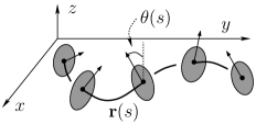
Figure 2: Geometry of the constrained rod

Consider an inextensible Cosserat rod of length $\ell$ equipped with three directors. If we denote the centerline at time $t$ as $s\mapsto\mathbf{r}(t,s)$, inextensibility allows us to assume that the parameter $s$ is the arclength. Secondly, we can take the director frame $\{\mathbf{d}_{1},\mathbf{d}_{2},\mathbf{d}_{3}\}$ to be orthonormal, such that $\mathbf{d}_{1}$ is the unit tangent vector $\mathbf{r}^{\prime}$. We will not take the effect of gravity into account.

In addition, we now assume that the centerline is a planar curve moving in the horizontal $(x,y)$-plane, i.e. $\mathbf{r}(t,s)$ can be written as $(x(t,s),y(t,s),0)$. We introduce the slope $\varphi(t,s)$ of the centerline as $(\cos\varphi,\sin\varphi)=(x^{\prime}(t,s),y^{\prime}(t,s))$. Furthermore, we define the angle $\theta(t,s)$, referred to as the torsion of the rod, as the angle subtended between $\mathbf{e}_{z}$ and $\mathbf{d}_{3}$. The director frame is completely determined once we know the slope $\varphi(s,t)$ and the torsion $\theta(s,t)$.

The specific constraints imposed on our rod model therefore allow us to eliminate the director frame in favour of the slope $\varphi$ and the torsion $\theta$. Furthermore, as we shall see, the slope $\varphi$ is related to the curvature of the centerline. Note that, in formulating the dynamics, we still have to impose the inextensibility condition $(x^{\prime})^{2}+(y^{\prime})^{2}=1$.

Remark 3.1.

Note that $\theta$ has nothing to do with the usual geometric concept of torsion of a curve in $\mathbb{R}^{3}$, and neither is $\theta$ related to the concept of shear in (for example) the theory of the Timoshenko beam. $\diamond$

3.2 The dynamics

As the director frame is orthonormal, there exists a vector $\mathbf{u}$, defined by $\mathbf{d}^{\prime}_{i}=\mathbf{u}\times\mathbf{d}_{i}$, called the strain or Darboux vector. With the conventions from the previous section, $\mathbf{u}$ takes the following form:

$$\mathbf{u}=\theta^{\prime}\mathbf{d}_{1}+\varphi^{\prime}\mathbf{e}_{z}.$$

($\mathbf{u}$ can be thought of as an “angular momentum” vector, but with time-derivatives replaced by derivatives with respect to arclength.)

The dynamics of our rod model can be derived from a variational principle. The kinetic energy is given by

$$T=\frac{1}{2}\int_{0}^{\ell}\left(\rho(s)(\dot{x}^{2}+\dot{y}^{2})+\alpha\dot{\theta}^{2}\right)\,\mathrm{d}s,$$

where $\alpha$ is an appropriately chosen constant. Here, the mass density is denoted by $\rho$, and will be assumed constant from now on.

For a hyperelastic rod, the potential energy is of the form

$$V=\int_{0}^{\ell}W(u_{1},u_{2},u_{3})\mathrm{d}s,$$

where $W(u_{1},u_{2},u_{3})$ is called the stored energy density, and the $u_{i}$ are the components of $\mathbf{u}$ relative to the director frame: $u_{i}=\mathbf{u}\cdot\mathbf{d}_{i}$. In the simplest case, of linear elasticity, $W$ is a quadratic function of the strains:

$$W(u_{1},u_{2},u_{3})=\frac{1}{2}\left(K_{1}u_{1}^{2}+K_{2}u_{2}^{2}+K_{3}u_{3}^{2}\right).$$ (16)

We will not dwell on the physical interpretation of the constants $K_{i}$ any further (in this case, they are related to the moments of inertia of the laminae). If the rod is transversely isotropic, i.e. if the laminae are invariant under rotations around $\mathbf{d}_{1}$, we may take $K_{2}=K_{3}$. The potential energy then becomes

$$V=\frac{1}{2}\int_{0}^{\ell}\left(\beta(\theta^{\prime})^{2}+K\kappa^{2}\right)\mathrm{d}s,$$ (17)

where $\kappa$ is the curvature of the centerline, i.e. $\kappa^{2}=(\varphi^{\prime})^{2}=(x^{\prime\prime})^{2}+(y^{\prime\prime})^{2}$, and where we have put $\beta:=K_{1}$ and $K:=K_{2}$. Models with a similar potential energy abound throughout the literature and are generally referred to as the Euler elastica. For more information, see [23] and the references therein.

3.3 The second-order model

Having eliminated the derivative of the slope $\varphi$ from the stored energy density, we end up with a model in which the fields are the coordinates of the centerline $(x(t,s),y(t,s))$ and the torsion angle $\theta(t,s)$. This model fits into the framework developed in section 2.2.2; the base space $X$ is $\mathbb{R}^{2}$, with coordinates $(t,s)$ and the total space $Y$ is $X\times\mathbb{R}^{2}\times\mathbb{S}^{1}$, with fibre coordinates $(x,y,\theta)$.

The total Lagrangian now consists of the density of kinetic energy minus that of potential energy, as well as an additional term enforcing the constraint of inextensibility, and can be written as

$$L=\frac{\rho}{2}(\dot{x}^{2}+\dot{y}^{2})+\frac{\alpha}{2}\dot{\theta}^{2}-\frac{1}{2}\left(\beta(\theta^{\prime})^{2}+K\kappa^{2}\right)-\frac{1}{2}p\left((x^{\prime})^{2}+(y^{\prime})^{2}-1\right),$$ (18)

where $p$ is a Lagrange multiplier associated to the constraint of inextensibility. The field equations associated to this Lagrangian take the following form:

$$\left\{\begin{array}[]{rcl}\rho\ddot{x}+Kx^{\prime\prime\prime\prime}&=&\frac{\partial}{\partial s}(px^{\prime})\\ \rho\ddot{y}+Ky^{\prime\prime\prime\prime}&=&\frac{\partial}{\partial s}(py^{\prime})\\ \alpha\ddot{\theta}-\beta\theta^{\prime\prime}&=&0,\end{array}\right.$$ (19)

to be supplemented with the inextensibility constraint

$$(x^{\prime})^{2}+(y^{\prime})^{2}=1,$$ (20)

which allows to determine the multiplier $p$. Note in passing that the dynamics of the centerline and the torsion angle $\theta$ are completely uncoupled. This will change once we add nonholonomic constraints.

3.4 Field equations and symmetries

We recall the expression (2.2.2) for the second-order Cartan form. If a Lie group $G$ is acting on $Y$ by bundle automorphisms, and on $J^{3}\pi$ by prolonged bundle automorphisms, there is a Lagrangian momentum map $J^{L}_{\xi}=\xi_{J^{3}\pi}\vrule height=0.0pt,depth=0.4pt,width=3.0pt\vrule height=7.0pt,depth=0.4pt\kern 3.0pt\Omega_{L}$, as described in section 2.2. We now turn to a brief overview of the symmetries associated to the rod model introduced in the previous section. For an overview of symmetries in the general theory of Cosserat rods, see [24].

Translations in time

The Lie group $\mathbb{R}$ acts on $X$ by translations in time: $\Phi_{\epsilon}:(s,t)\mapsto(s,t+\epsilon)$. The Lagrangian is invariant and the pullback to $X$ (by a solution $j^{3}\phi$ of the field equations) of the momentum map associated to the infinitesimal generator $\frac{\partial}{\partial t}$ is given by

$$(j^{3}\phi)^{\ast}J^{L}_{1}=\left[(px^{\prime}-Kx^{\prime\prime\prime})\dot{x}+(py^{\prime}-Ky^{\prime\prime\prime})\dot{y}+\beta\theta^{\prime}\dot{\theta}+K(x^{\prime\prime}\dot{x}^{\prime}+y^{\prime\prime}\dot{y}^{\prime})\right]\mathrm{d}t$$ (21)

$$\hbox to0.0pt{\hss${}+{}$}\big{[}\underbrace{\frac{\rho}{2}(\dot{x}^{2}+\dot{y}^{2})+\frac{\alpha}{2}\dot{\theta}^{2}+\frac{K}{2}((x^{\prime\prime})^{2}+(y^{\prime\prime})^{2})+\frac{\beta}{2}(\theta^{\prime})^{2}+\frac{p}{2}((x^{\prime})^{2}+(y^{\prime})^{2}-1)}_{\mathcal{E}}\big{]}\mathrm{d}s,$$

where we have introduced the energy density $\mathcal{E}$. By taking the exterior derivative of (21) and integrating the conservation law $\mathrm{d}[(j^{3}\phi)^{\ast}J^{L}_{1}]=0$ over $[0,\ell]\times[t_{0},t_{1}]\subset\mathbb{R}^{2}$, we obtain

$$E(t_{1})-E(t_{0})=\int_{t_{0}}^{t_{1}}\left[(px^{\prime}-Kx^{\prime\prime\prime})\dot{x}+(py^{\prime}-Ky^{\prime\prime\prime})\dot{y}+\beta\theta^{\prime}\dot{\theta}+K(x^{\prime\prime}\dot{x}^{\prime}+y^{\prime\prime}\dot{y}^{\prime})\right]^{\ell}_{0}\mathrm{d}t,$$ (22)

where $E(t)=\int_{0}^{\ell}\mathcal{E}\mathrm{d}s$ is the total energy, which is conserved if suitable boundary conditions are imposed. This is the case, for instance, for periodic boundary conditions or when both ends of the rod can move freely, i.e. when

$$px^{\prime}-Kx^{\prime\prime\prime}=py^{\prime}-Ky^{\prime\prime\prime}=0\quad\mathrm{and}\quad x^{\prime\prime}=y^{\prime\prime}=\theta^{\prime}=0\quad\mbox{at $s=0,\ell$}.$$

Spatial translations

Consider the Abelian group $\mathbb{R}^{2}$ acting on the total space $Y$ by translation, i.e. for each $(a,b)\in\mathbb{R}^{2}$ we consider the map $\Phi_{(a,b)}:(s,t;x,y,\theta)\mapsto(s,t;x+a,y+b,\theta)$. The Lagrangian density is invariant under this action and the associated momentum map is

$$(j^{3}\phi)^{\ast}J^{L}_{(v_{1},v_{2})}=-\rho(v_{1}\dot{x}+v_{2}\dot{y})\mathrm{d}s-(v_{1}px^{\prime}-v_{1}Kx^{\prime\prime\prime}+v_{2}py^{\prime}-v_{2}Ky^{\prime\prime\prime})\mathrm{d}t$$

for all $(v_{1},v_{2})\in\mathbb{R}^{2}$. Again, under suitable boundary conditions, $J^{L}_{(v_{1},v_{2})}$ gives rise to a conserved quantity, namely the total linear momentum of the rod.

Similarly, $\mathbb{S}^{1}$ acts on $Y$ by translations in $\theta$, with infinitesimal generator of the form $\frac{\partial}{\partial\theta}$, and the corresponding momentum map is

$$(j^{3}\phi)^{\ast}J^{L}_{1}=-\beta\theta^{\prime}\mathrm{d}t-\alpha\dot{\theta}\mathrm{d}s.$$

The ensuing conservation law is given by $\alpha\ddot{\theta}=\beta\theta^{\prime\prime}$ and, hence, is just the equation of motion for $\theta$.

Spatial rotations

Finally, we note that the rotation group $SO(2)$ acts on $Y$ by rotations in the $(x,y)$-plane. The infinitesimal generator corresponding to $1\in\mathfrak{so}(2)\cong\mathbb{R}$ is given by $y\frac{\partial}{\partial x}-x\frac{\partial}{\partial y}$; its prolongation to $J^{3}\pi$ is

$$\xi_{J^{3}\pi}=y\frac{\partial}{\partial x}-x\frac{\partial}{\partial y}+\dot{y}\frac{\partial}{\partial\dot{x}}-\dot{x}\frac{\partial}{\partial\dot{y}}+y^{\prime}\frac{\partial}{\partial x^{\prime}}-x^{\prime}\frac{\partial}{\partial y^{\prime}}+\cdots,$$

where the dots represent terms involving higher-order derivatives. As $\Theta_{L}$ is semibasic with respect to $\pi_{3,1}$, these terms make no contribution to the momentum map. The momentum map is given by

$$(j^{3}\phi)^{\ast}J^{L}_{1}=\left[-x(-py^{\prime}+Ky^{\prime\prime\prime})+y(-px^{\prime}+Kx^{\prime\prime\prime})-K(x^{\prime\prime}y^{\prime}+y^{\prime\prime}x^{\prime})\right]\mathrm{d}t+\rho(x\dot{y}-y\dot{x})\mathrm{d}s,$$

leading to the conservation of total angular momentum. Note that the angular momentum does not involve $\theta$, in contrast to the corresponding expression in more general treatments of Cosserat media. This is a consequence of the fact that we defined the action of $SO(2)$ on $Y$ to act trivially on the $\theta$ part.

3.5 A nonholonomic model

Consider again a Cosserat rod as in the previous section. The constraint that we are now about to introduce is a generalization of the familiar concept of rolling without sliding in mechanics: we assume that the rod is placed on a horizontal plane, which we take to be perfectly rough, so that each of the laminae rolls without sliding.

However, as the Cosserat rod is also supposed to be incompressible, one must take care that the additional constraints do not become too restrictive. Indeed, a simple argument shows that the model of an incompressible rod which rolls without sliding, and which cannot move transversally, can only move like a rigid body.

There are two immediate solutions: either one relaxes the incompressibility constraint, or one allows the rod to move laterally as well. Either solution introduces a lot of mathematical tedium which greatly obscures the physical background of the system. For this paper, we will therefore consider a simplified model containing aspects of both models.

In particular, we will assume that the motion of the nonholonomic rod is such that the incompressibility constraint is satisfied approximately throughout the motion; this is equivalent to the following assumption:

$$\sqrt{(x^{\prime})^{2}+(y^{\prime})^{2}}\cong 1.$$ (23)

By neglecting the incompressibility constraint in the Lagrangian, a simplified model is then obtained. Of course, this new model is a mathematical simplification of the true physics. However, numerical simulations show that $\sqrt{(x^{\prime})^{2}+(y^{\prime})^{2}}$ is bounded throughout the motion, and it’s therefore reasonable that the dynamics of this model is close to the true dynamics. One could think of the mathematical model as describing a Cosserat rod whose constitutive equation is specified on mathematical grounds, rather than derived from first principles.

The constraints of rolling without sliding are given by (see [25, 26]):

$$\dot{x}+R\dot{\theta}\sin\varphi=0\quad\mathrm{and}\quad\dot{y}-R\dot{\theta}\cos\varphi=0,$$ (24)

where $R$ is the radius of the laminae. By eliminating the slope $\varphi$ we then obtain

$$\dot{x}+R\dot{\theta}y^{\prime}=0\quad\mathrm{and}\quad\dot{y}-R\dot{\theta}x^{\prime}=0.$$ (25)

Incidentally, the passage from (24) to (25) again illustrates why derivatives with respect to time play a fundamentally different role as opposed to the other derivatives.

The Lagrangian density of the nonholonomic rod is still given by (18); we recall that it is of second order, as the stored energy function (16) is of grade two. The constraint on the other hand is of first order. By demanding that the action be stationary under variations compatible with the given constraint (a similar approach to section 2.3), we obtain the following field equations:

Definition 3.2.

A section $\phi$ of $\pi$ is a solution of the nonholonomic problem if and only if $\mathrm{Im}\,j^{1}\phi\subset\mathcal{C}$, and, along $\mathcal{C}$,

$$(j^{3}\phi)^{\ast}(j^{3}V\vrule height=0.0pt,depth=0.4pt,width=3.0pt\vrule height=7.0pt,depth=0.4pt\kern 3.0pt\Omega_{L})=0$$ (26)

for all $\pi$-vertical vector fields $V$ on $Y$ such that $(j^{1}\phi)^{\ast}(j^{1}V\vrule height=0.0pt,depth=0.4pt,width=3.0pt\vrule height=7.0pt,depth=0.4pt\kern 3.0pt\alpha)=0$ for all $\alpha\in F$.

The left-hand side of (26) is just the Euler-Lagrange equation (10) for a second-order Lagrangian. As the constraint is first order, it can be treated exactly as in section 2.3. In coordinates, the nonholonomic field equations hence are given by

$$\left[\frac{\partial L}{\partial y^{a}}-\frac{\mathrm{d}}{\mathrm{d}x^{\mu}}\left(\frac{\partial L}{\partial y^{a}_{\mu}}\right)+\frac{\mathrm{d}^{2}}{\mathrm{d}x^{\mu}\mathrm{d}x^{\nu}}\left(\frac{\partial L}{\partial y^{a}_{\mu\nu}}\right)\right](j^{4}\phi)=\lambda_{\alpha}\frac{\partial\varphi^{\alpha}}{\partial y^{a}_{0}}(j^{1}\phi).$$

By substituting the Lagrangian (18), without the inextensibility constraint, and the constraints (25) into the Euler-Lagrange equations, we obtain the following set of nonholonomic field equations:

$$\left\{\begin{array}[]{rcl}\rho\ddot{x}+Kx^{\prime\prime\prime\prime}&=&\lambda\\ \rho\ddot{y}+Ky^{\prime\prime\prime\prime}&=&\mu\\ \alpha\ddot{\theta}-\beta\theta^{\prime\prime}&=&R(\lambda y^{\prime}+\mu x^{\prime})\end{array}\right.$$ (27)

where $\lambda$ and $\mu$ are Lagrange multipliers associated with the nonholonomic constraints. These equations are to be supplemented by the constraint equations (25).

In the familiar case of the rolling disc, it is well known that energy is conserved. There is a similar conservation law for the nonholonomic rod.

Proposition 3.3.

The total energy (22) is conserved for each solution of the nonholonomic field equations (27) and constraints (25). A fortiori, the solutions of the nonholonomic field equations satisfy the local conservation law $\mathrm{d}[(j^{3}\phi)^{\ast}J^{L}_{1}]=0$, where $J^{L}_{1}$ is the momentum map associated to time translation introduced in (21).

Proof:  This follows immediately from proposition 6.1 in the appendix, and the fact that $\frac{\partial}{\partial t}$ (or rather its prolongation to $J^{1}\pi$) annihilates $\bar{F}$ along the constraint manifold. Indeed, the bundle of $(n+1)$-forms $\bar{F}$ is generated by $\Phi^{1}$ and $\Phi^{2}$, defined as follows:

$$\Phi^{1}=(\mathrm{d}x-\dot{x}\mathrm{d}t)\wedge\mathrm{d}s+Ry^{\prime}(\mathrm{d}\theta-\dot{\theta}\mathrm{d}t)\wedge\mathrm{d}s;$$

$$\Phi^{2}=(\mathrm{d}y-\dot{y}\mathrm{d}t)\wedge\mathrm{d}s-Rx^{\prime}(\mathrm{d}\theta-\dot{\theta}\mathrm{d}t)\wedge\mathrm{d}s.$$

Therefore, we have that

$$\left(\frac{\partial}{\partial t}\right)_{J^{1}\pi}\vrule height=0.0pt,depth=0.4pt,width=3.0pt\vrule height=7.0pt,depth=0.4pt\kern 3.0pt\Phi^{1}=-(\dot{x}+R\dot{\theta}y^{\prime})\mathrm{d}s,$$

which vanishes when restricted to $\mathcal{C}$. A similar argument shows that the contraction of $\frac{\partial}{\partial t}$ with $\Phi^{2}$ vanishes. Hence, proposition 6.1 can be applied; the associated momentum map is just (21). $\Box$

4 Discrete nonholonomic field theories

In this section we present an extension to the case of field theories of the discrete d’Alembert principle described in [27]. We also study an elementary numerical integration scheme aimed at integrating the field equations (27).

As in the previous sections, we will consider the trivial bundle $\pi$ with base space $X=\mathbb{R}\times M$ (where $M=[0,\ell]$), and total space $Y$ the product $X\times S$, where $S=\mathbb{R}^{2}\times\mathbb{S}^{1}$. Our discretization scheme is the most straightforward possible: The base space $X$ will be discretized by means of the uniform mesh $\mathbb{Z}\times\mathbb{Z}$, and the total space $Y$ by replacing it with $X\times\mathbb{R}^{2}\times\mathbb{R}$.

4.1 Discrete Lagrangian field theories

We begin by giving an overview of discrete Lagrangian field theories, inspired by [21, 28]. In order to discretize the second-order jet bundle, we need to approximate the derivatives of the field (of first and second order). This we do by means of central differences with spatial step $k$ and time step $h$:

$$\dot{\eta}\approx\frac{\eta_{n+1,i}-\eta_{n,i}}{h},\quad\eta^{\prime}\approx\frac{\eta_{n,i+1}-\eta_{n,i-1}}{2k},\quad\mathrm{and}\quad\eta^{\prime\prime}\approx\frac{\eta_{n,i+1}-2\eta_{n,i}+\eta_{n,i-1}}{k^{2}},$$ (28)

where $\eta$ stands for either $x$ or $y$. Other derivatives will not be needed. For $\theta$, we use

$$\dot{\theta}\approx\frac{\theta_{n+1,i}-\theta_{n,i}}{h}\quad\mathrm{and}\quad\theta^{\prime}\approx\frac{\theta_{n,i+1}-\theta_{n,i}}{k}.$$ (29)

Let $\mathcal{M}$ be the uniform mesh in $X=\mathbb{R}^{2}$ whose elements are points with integer coordinates; i.e. $\mathcal{M}=\mathbb{Z}\times\mathbb{Z}$. The elements of $\mathcal{M}$ are denoted as $(n,i)$, where the first component refers to time, and the second to the spatial coordinate. We define a $9$-cell centered at $(n,i)\in\mathcal{M}$, denoted by $[x]_{(n,i)}$, to be a nine-tuple of the form

$$[x]_{(n,i)} := \big{(}(n-1,i-1),(n-1,i),(n-1,i);(n,i-1),$$

$$(n,i),(n,i+1);(n+1,i-1),(n+1,i),(n+1,i+1)\big{)}$$

It is clear from the finite difference approximations that a generic second-order jet $j^{2}_{x}\phi$ can be approximated by specifying the values of $\phi$ at the nine points of a cell.

However, in the case of the nonholonomic rod, the Lagrangian depends only on the derivative coordinates whose finite difference approximations were given in (28) and (29). Therefore, we can simplify our exposition by defining a $6$-cell at $(n,i)$ to be the six-tuple

$$[x]_{(n,i)}:=\big{(}(n,i-1),(n,i),(n,i+1);(n+1,i-1),(n+1,i),(n+1,i+1)\big{)}.$$ (31)

We will refer to $6$-cells simply as cells. Let us denote the set of all cells by $\mathbb{X}^{6}:=\{[x]_{(n,i)}:(n,i)\in\mathcal{M}\}$. We now define the discrete $2$nd order jet bundle to be $J^{2}_{d}\pi:=\mathbb{X}^{6}\times S^{6}$ (see [21, 28, 29]). A discrete section of $\pi$ (also referred to as a discrete field) is a map $\phi:\mathcal{M}\rightarrow S$. Its second jet extension is the map $j^{2}\phi:\mathbb{X}^{6}\rightarrow J^{2}_{d}\pi$ defined as

$$j^{2}\phi([x]_{(n,i)}):=([x]_{(n,i)};\phi(x_{1}),\ldots\phi(x_{6})),$$

where $x_{1},\ldots,x_{6}$ are the vertices that make up $[x]_{(n,i)}$ (ordered as in (31)). Given a vector field $W$ on $Y$, we define its second jet extension to be the vector field $j^{2}W$ on $J^{2}_{d}$ given by

$$j^{2}W([x];f_{1},\ldots,f_{6})=(W(x_{1},f_{1}),W(x_{2},f_{2}),\ldots,W(x_{6},f_{6})).$$

Let us now assume that a discrete Lagrangian $L_{d}:J^{2}_{d}\pi\rightarrow\mathbb{R}$ is given. The action sum $S_{d}$ is then defined as

$$S_{d}(\phi)=\sum_{[x]}L_{d}(j^{2}\phi([x])).$$ (32)

Given a vertical vector field $V$ on $Y$ and a discrete field $\phi$, we obtain a one-parameter family $\phi_{\epsilon}$ by composing $\phi$ with the flow $\Phi$ of $V$:

$$\phi_{\epsilon}([x])=\left([x];\Phi_{\epsilon}(\phi([x])_{1}),\ldots,\Phi_{\epsilon}(\phi([x])_{6})\right).$$ (33)

The variational principle now consists of seeking discrete fields $\phi$ that extremize the discrete action sum. The fact that $\phi$ is an extremum of $S$ under variations of the form (33) is expressed by

$$\sum_{(n,i)\in\mathcal{M}}\Big{<}X(\phi_{(n,i)}),D_{1}L(j^{2}\phi([x]_{(n,i+1)}))+D_{2}L(j^{2}\phi([x]_{(n,i)}))+D_{3}L(j^{2}\phi([x]_{(n,i-1)}))$$ (34)

$$\hbox to0.0pt{\hss${}+{}$}D_{4}L(j^{2}\phi([x]_{(n-1,i+1)}))+D_{5}L(j^{2}\phi([x]_{(n-1,i)}))+D_{6}L(j^{2}\phi([x]_{(n-1,i-1)}))\Big{>}=0.$$

As the variation $X$ is completely arbitrary, we obtain the following set of discrete Euler-Lagrange field equations:

$$D_{1}L(j^{2}\phi([x]_{(n,i+1)}))+D_{2}L(j^{2}\phi([x]_{(n,i)}))+D_{3}L(j^{2}\phi([x]_{(n,i-1)}))+$$ (35)

$$D_{4}L(j^{2}\phi([x]_{(n-1,i+1)}))+D_{5}L(j^{2}\phi([x]_{(n-1,i)}))+D_{6}L(j^{2}\phi([x]_{(n-1,i-1)}))=0.$$

for all $(n,i)$. Here, we have denoted the values of the field $\phi$ at the points $(n,i)$ as $\phi_{n,i}$.

4.2 The discrete d’Alembert principle

Our discrete d’Alembert principle is nothing more than a suitable field-theoretic extension of the discrete Lagrange-d’Alembert principle described in [27]. Just as in that paper, in addition to the discrete Lagrangian $L_{d}$, two additional ingredients are needed: a discrete constraint manifold $\mathcal{C}_{d}\subset J^{1}_{d}\pi$ and a bundle of constraint forces $F_{d}$ on $J^{2}_{d}\pi$. However, as our constraints (in particular (25)) are not linear in the derivatives, as opposed to the case in [27], our analysis will be more involved.

The discrete constraint manifold $\mathcal{C}_{d}\hookrightarrow J^{1}_{d}\pi$ will usually be constructed from the continuous constraint manifold $\mathcal{C}$ by subjecting it to the same discretization as used for the discretization of the Lagrangian (i.e. (28) and (29)). To construct the discrete counterpart $F_{d}$ of the bundle of discrete constraint forces, somewhat more work is needed.

Remark 4.1.

For the discretization of the constraint manifold, it would appear that we need a discrete version of the first-order jet bundle as well. A similar procedure as for the discretization of the second-order jet bundle (using the same finite differences as in (28) shows that a discrete $1$-jet depends on the values of the field at the same four points of a cell as a discrete $2$-jet: the difference between $J^{1}_{d}\pi$ and $J^{2}_{d}\pi$ lies in the way in which the values of the field at these points are combined. Therefore, we can regard the discrete version of $\mathcal{C}$, to be defined below, as a subset of $J^{2}_{d}\pi$. $\diamond$

4.2.1 The bundle of discrete constraint forces

In this section, we will construct $F_{d}$ by following a discrete version of the procedure used in section 2.3. Just as in the continuous case, it is here that the difference between spatial and time derivatives will become fundamental. Indeed, we will discretize with respect to space first, and (initially) not with respect to time. It should be noted that the construction outlined in this paragraph is not entirely rigorous but depends strongly on coordinate expressions. Presumably, one would need a sort of discrete Cauchy analysis in order to solidify these arguments. For now, we will just accept that this reasoning provides us with the correct form of the constraint forces.

For the sake of convenience, we suppose that $\mathcal{C}$ is given by the vanishing of $k$ independent functions $\varphi^{\alpha}$ on $J^{1}\pi$. By applying the spatial discretizations in (28) and (29) to $\varphi^{\alpha}$, we obtain $k$ functions, denoted as $\varphi^{\alpha}_{1/2}$, on $J^{2}_{d}\times TS$. We define the semi-discretized constraint submanifold $\mathcal{C}_{1/2}$ to be the zero level set of the functions $\varphi^{\alpha}_{1/2}$.

Consider now the forms

$$\Phi^{\alpha}_{1/2}:=J^{\ast}(\mathrm{d}\varphi^{\alpha}_{1/2})$$

(where $J$ is the vertical endomorphism on $TS$); they are the semi-discrete counterparts of the forms $\Phi^{\alpha}$ defined in (15). The forms $\Phi^{\alpha}_{1/2}$ are semi-basic. By discretizing the time derivatives, however, we obtain a set of basic forms on $J^{2}_{d}\pi$, which we also denote by $\Phi^{\alpha}_{1/2}$. An example will make this clearer.

Example 4.2.

Consider, for instance, the constraint manifold $\mathcal{C}\hookrightarrow J^{2}\pi$ defined as the zero level set of the function $\varphi=A_{ab}\,y^{a}_{0}y^{b}_{1}+B_{b}(y^{b}_{1})^{2}$, where $A_{ab}$ and $B_{b}$ are constants. By applying (28) and (29), it follows that $\mathcal{C}_{d}$ is given as the zero level set of the function

$$\varphi_{d}([y]):=A_{ab}\frac{y^{a}_{n+1,i}-y^{a}_{n,i}}{h}\frac{y^{b}_{n,i+1}-y^{b}_{n,i-1}}{2k}+B_{b}\left(\frac{y^{b}_{n,i+1}-y^{b}_{n,i-1}}{2k}\right)^{2}$$

for $[y]\in J^{1}_{d}\pi$, and $\mathcal{C}_{1/2}$ as the zero level set of the function

$$\varphi_{1/2}([y],v):=A_{ab}\,\dot{v}^{a}\,\frac{y^{b}_{n,i+1}-y^{b}_{n,i-1}}{2k}+B_{b}\left(\frac{y^{b}_{n,i+1}-y^{b}_{n,i-1}}{2k}\right)^{2}$$

for $[y]\in J^{1}_{d}\pi$ and $v\in TS$. The bundle $F_{d}$ is then generated by the one-form $\Phi_{1/2}:=S^{\ast}(\mathrm{d}\varphi_{1/2})$, or explicitly,

$$\Phi=A_{ab}\frac{y^{b}_{n,i+1}-y^{b}_{n,i-1}}{2k}\mathrm{d}y^{a}.$$

4.2.2 The discrete nonholonomic field equations

Assuming that $L_{d}$, $\mathcal{C}_{d}$ and $F_{d}$ are given (their construction will be treated in more detail in the next section), the derivation of the discrete nonholonomic field equations is similar to the continuum derivation: we are looking for a discrete field $\phi$ such that $\mathrm{Im}\,j^{1}\phi\subset\mathcal{C}_{d}$ and such that $\phi$ is an extremum of (32) for all variations compatible with the constraints, in the sense that the variation $X$ satisfies, for all $(n,i)$,

$$X(\phi_{(n,i)})\vrule height=0.0pt,depth=0.4pt,width=3.0pt\vrule height=7.0pt,depth=0.4pt\kern 3.0pt\Phi^{\alpha}_{1/2}(j^{2}\phi([x]_{(n,i)}))=0.$$

From (34) we then obtain the discrete nonholonomic field equations:

$$D_{1}L(j^{2}\phi([x]_{(n,i+1)}))+D_{2}L(j^{2}\phi([x]_{(n,i)}))+D_{3}L(j^{2}\phi([x]_{(n,i-1)}))+D_{4}L(j^{2}\phi([x]_{(n-1,i+1)}))$$

$$\hbox to0.0pt{\hss${}+{}$}D_{5}L(j^{2}\phi([x]_{(n-1,i)}))+D_{6}L(j^{2}\phi([x]_{(n-1,i-1)}))=\lambda_{\alpha}\Phi^{\alpha}_{1/2}(j^{2}\phi([x]_{(n,i)})),$$ (36)

where the Lagrange multipliers $\lambda_{\alpha}$ are to be determined from the requirement that $\mathrm{Im}\,j^{2}\phi\subset\mathcal{C}_{d}$.

4.3 An explicit, second-order algorithm

In this section, we briefly present some numerical insights into the nonholonomic field equations of section 3.5. Our aim is twofold: for generic boundary conditions, the nonholonomic field equations (27) cannot be solved analytically and in order to gain insight into the behaviour of our model, we therefore turn to numerical methods. Secondly, in line with the fundamental tenets of geometric integration, we wish to show that the construction of practical integration schemes is strongly guided by geometric principles.

In discretizing our rod model, we effectively replace the continuous rod by $N$ rigid rolling discs interconnected by some potential (see [30]). This is again an illustration of the fact that the constraints are truly nonholonomic. Our integrator is just a concatenation of the leapfrog algorithm for the spatial part, and a nonholonomic mechanical integrator for the integration in time.

As a first attempt at integrating (27), we present an explicit, second-order algorithm. In the Lagrangian, the derivatives are approximated by

$$\dot{x}\approx\frac{x_{n+1,i}-x_{n,i}}{h}\quad\mathrm{and}\quad x^{\prime\prime}\approx\frac{x_{n,i-1}-2x_{n,i}+x_{n+1,i}}{k^{2}},$$

where $h$ is the time step, and $k$ is the space step. Similar approximations are used for the derivatives of $y$, and for $\theta$ we use

$$\dot{\theta}\approx\frac{\theta_{n+1,i}-\theta_{n,i}}{h}\quad\mathrm{and}\quad\theta^{\prime}\approx\frac{\theta_{n,i+1}-\theta_{n,i}}{k}.$$ (37)

The discrete Lagrangian density can then be found by substituting these approximations into the continuum Lagrangian (18). Explicitly, it is given by

$$L_{d}=\frac{\rho}{2h^{2}}\left((x_{n+1,i}-x_{n,i})^{2}+(y_{n+1,i}-y_{n,i})^{2}\right)+\frac{\alpha}{2h^{2}}(\theta_{n+1,i}-\theta_{n,i})^{2}-\frac{\beta}{2k^{2}}(\theta_{n,i+1}-\theta_{n,i})^{2}$$

$$\hbox to0.0pt{\hss${}-{}$}\frac{K}{2k^{4}}(x_{n,i-1}-2x_{n,i}+x_{n,i+1})^{2}-\frac{K}{2k^{4}}(y_{n,i-1}-2y_{n,i}+y_{n,i+1})^{2}.$$ (38)

Note that $L_{d}$ only depends on four of the six points in each cell (see (31)). The discrete constraint manifold $\mathcal{C}_{d}$ is found by discretizing the constraint equations (25). In order to obtain a second-order accurate approximation, we use central differences:

$$x^{\prime}\approx\frac{x_{n,i+1}-x_{n,i-1}}{2k},$$

(and similar for $y^{\prime},\dot{x},\dot{y},\dot{\theta}$) and hence we obtain that $\mathcal{C}_{d}$ is given by

$$x_{n+1,i}-x_{n-1,i}+\frac{R}{2k}(\theta_{n+1,i}-\theta_{n-1,i})(y_{n,i+1}-y_{n,i-1})=0,$$ (39)

and

$$y_{n+1,i}-y_{n-1,i}-\frac{R}{2k}(\theta_{n+1,i}-\theta_{n-1,i})(x_{n,i+1}-x_{n,i-1})=0,$$ (40)

for all $(n,i)$. The semi-discrete constraint manifold $\mathcal{C}_{1/2}$, on the other hand, is given by

$$\dot{x}_{n,i}+\frac{R}{2k}\dot{\theta}_{n,i}(y_{n,i+1}-y_{n,i-1})=0,$$

and

$$\dot{y}_{n,i}-\frac{R}{2k}\dot{\theta}_{n,i}(x_{n,i+1}-x_{n,i-1})=0,$$

and hence $F_{d}$ is generated by

$$\Phi^{1}=\mathrm{d}x+\frac{R}{2k}(y_{n,i+1}-y_{n,i-1})\mathrm{d}\theta\quad\mathrm{and}\quad\Phi^{2}=\mathrm{d}y-\frac{R}{2k}(x_{n,i+1}-x_{n,i-1})\mathrm{d}\theta.$$

We conclude that the discrete nonholonomic field equations (36) are in this case

$$x_{n+1,i}-2x_{n,i}+x_{n-1,i}=h^{2}\lambda_{i}-\frac{h^{2}K}{k^{4}}\Delta^{4}x_{n,i}$$ (41)

and

$$y_{n+1,i}-2y_{n,i}+y_{n-1,i}=h^{2}\mu_{i}-\frac{h^{2}K}{k^{4}}\Delta^{4}y_{n,i}$$ (42)

as well as

$$\alpha(\theta_{n+1,i}-2\theta_{n,i}+\theta_{n-1,i})=Rh^{2}\left(\lambda_{i}\frac{y_{n,i+1}-y_{n,i-1}}{2k}-\mu_{i}\frac{x_{n,i+1}-x_{n,i-1}}{2k}\right)+\frac{\beta h^{2}}{k^{2}}\Delta^{2}\theta_{n,i},$$

where $\Delta^{2}$ and $\Delta^{4}$ are the 2nd and 4th order finite difference operators in the spatial direction, respectively:

$$\Delta^{2}f_{n,i}:=f_{n,i+1}-2f_{n,i}+f_{n,i-1}$$

and

$$\Delta^{4}f_{n,i}:=f_{n,i+2}-4f_{n,i+1}+6f_{n,i}-4f_{n,i-1}+f_{n,i-2}.$$

In order to determine $\lambda_{i}$ and $\mu_{i}$, these equations need to be supplemented by the discrete constraints (39) and (40).

For the purpose of numerical simulation, the following values were used: $\alpha=1$, $\beta=0.8$, $\rho=1$, $K=0.7$, $\ell=4$, and $R=1$. For the spatial discretization, $32$ points were used (corresponding to $k\approx 0.1290$) and the time step was set to $h=1/8k^{2}$, a fraction of the maximal allowable time step for the Euler-Bernoulli beam equation (see [31]). The ends of the rod were left free and the following initial conditions were used:

$$\mathbf{r}_{0}(s)=(s,0),\quad\theta_{0}(s)=-\frac{\pi}{2}\cos\frac{\pi s}{\ell}\quad\mathrm{and}\quad\dot{\mathbf{r}}_{0}(s)=(0,0),\quad\dot{\theta}_{0}(s)=0.$$

An mpeg movie (created with Povray, an open source raytracer) depicting the motion of the nonholonomic Cosserat rod is available from the author’s web page. In figure 3, an impression of the motion of the rod is given. The arrows represent the director field $\mathbf{d}_{3}$ and serve as an indication of the torsion. The rod starts from an initially straight, but twisted state and gradually untwists, meanwhile effecting a rotation.

In figure 4, the energy of the nonholonomic rod is plotted. Even though our algorithm is by its very nature not symplectic (or multi-symplectic – see [32]), there is still the similar behaviour of “almost” energy conservation.

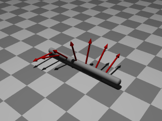
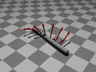
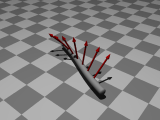
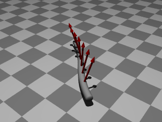
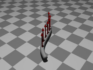
Figure 3: Motion of the rod from $t=0$ to $t\approx 4.5$.

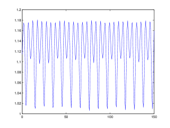
Figure 4: Energy behaviour of the integration algorithm on moderate time scales (the interval $[0,150]$).

5 Conclusions

It is clear that the study of nonholonomic field theories forms a vast subject. This paper gives only a brief survey of a number of straightforward results, but there are many more things to be explored. An acute problem is the lack of an extensive number of interesting examples; while this of course impedes progress on the theoretical front, there are nevertheless a number of points worth investigating, which we now discuss.

In proposition 3.3 we used the fact that the bundle of reaction forces is annihilated by the generator of time translations in order to prove conservation of energy. Even when this is not the case, experience from mechanics (see [33, 34, 35]) as well as from different types of nonholonomic field theories (see [36]) seems to suggest that it might be possible to prove a nonholonomic momentum equation instead.

From a numerical point of view, the explicit algorithm of section 4.3 is not very accurate. It is second-order in space and time and suffers from a restrictive stability condition. The development of more sophisticated integration schemes that exactly preserve the nonholonomic constraints would definitely be very interesting. Perhaps the most interesting of all, at least in line with the current investigations, would be a simulation of a nonholonomic model with a more physical constitutive equation than the one used in section 3.5.

6 Appendix: the nonholonomic Noether theorem

In the derivation of the Euler-Lagrange equations, both in the free as in the constrained case, we have restricted our attention to vertical variations. While it is well known that arbitrary variations do not yield any new information beyond the Euler-Lagrange equations (see [3]), the situation is not at all clear for nonholonomic field theories.

This is especially important for the derivation of the nonholonomic Noether theorem. Therefore, we propose the following modified bundle of reaction forces: if $F=\left<{A^{\alpha}_{a}\mathrm{d}y^{a}}\right>$, then

$$\bar{F}:=\left<{A^{\alpha}_{a}(\mathrm{d}y^{a}-y^{a}_{\mu}\mathrm{d}x^{\mu})\wedge\mathrm{d}^{n}x_{0}}\right>\subset\Omega^{(n+1)}(J^{1}\pi).$$ (43)

This situation is reminiscent of the comparison between Bridges’ $(n+1)$ multisymplectic $1$-forms and the Cartan $(n+1)$-form $\Theta_{L}$ in the work of Marsden and Shkoller [37], and is similar to the variational derivation of the Cartan form: if only vertical variations are taken into account, then the Cartan form is missing the $\mathrm{d}^{n+1}x$ term (see [3]).

The precise form of the bundle $\bar{F}$ can be derived by using arguments from Cauchy analysis (see [16]). The idea is to reformulate the field equations as a mechanical system on an infinite dimensional configuration space. The reaction forces can then be introduced in a straightforward way on this infinite-dimensional space, and by returning to the jet bundle one then obtains (43). The details of that derivation would lead us too far; more information on this technique will appear in a forthcoming publication (see also [38]). For now, we will simply accept the bundle $\bar{F}$ as given.

In [36] a similar type of bundle was used in the derivation of the nonholonomic momentum lemma. From that paper, we cite the following nonholonomic Noether theorem:

Proposition 6.1.

Let $L$ be a $G$-invariant Lagrangian density. Assume that $\xi\in\mathfrak{g}$ is such that $\xi_{J^{1}\pi}\vrule height=0.0pt,depth=0.4pt,width=3.0pt\vrule height=7.0pt,depth=0.4pt\kern 3.0pt\alpha=0$ along $\mathcal{C}$ for all $\alpha\in\bar{F}$. Then the following conservation law holds:

$$\mathrm{d}[(j^{1}\phi)^{\ast}J^{L}_{\xi}]=0,$$

for all sections $\phi$ of $\pi$ that are solutions of the nonholonomic field equations.

Note that a vertical vector $v$ belongs to $F^{\circ}$ if and only if $\left<{v,\alpha}\right>=0$ for all $\alpha\in\bar{F}$. Only for non-vertical vectors there is a difference between $F$ and $\bar{F}$. Therefore, if $\xi_{J^{1}\pi}$ in proposition 6.1 is vertical, then the nonholonomic Noether theorem follows from the Euler-Lagrange equations (2.9). In the other case, the techniques from [36] have to be used.

References

References

- [1] Bibbona E, Fatibene L and Francaviglia M 2006 Gauge-natural parameterized variational problems, vakonomic field theories and relativistic hydrodynamics of a charged fluid Int. J. Geom. Meth. Mod. Phys. 3 1573–1608
- [2] —–2006 Chetaev vs. vakonomic prescriptions in constrained field theories with parametrized variational calculus. Preprint math-ph/0608063
- [3] Marsden J E, Pekarsky S, Shkoller S, and West M 2001 Variational methods, multisymplectic geometry and continuum mechanics J. Geom. Phys. 38 253–84
- [4] Antman S S 2005 Nonlinear Problems of Elasticity (Berlin: Springer-Verlag)
- [5] García P L, García A and Rodrigo C 2006 Cartan forms for first order constrained variational problems, J. Geom. Phys. 56 571–610
- [6] Binz E, de León M, Martín de Diego D and Socolescu D 2002 Nonholonomic Constraints in Classical Field Theories Rep. Math. Phys. 49 151–66
- [7] Vankerschaver J, Cantrijn F, de León M and Martín de Diego D 2005 Geometric aspects of nonholonomic field theories Rep. Math. Phys. 56 387–411
- [8] Krupková O 2005 Partial differential equations with differential constraints J. Diff. Eq. 220 354–95
- [9] Krupková O and Volný P 2005 Euler-Lagrange and Hamilton equations for nonholonomic systems in field theory J. Phys. A: Math. Gen. 38 8715–45
- [10] Vignolo S and Bruno D 2002 Iper-ideal constraints in continuum mechanics J. Math. Phys. 43 325–43
- [11] Truesdell C and Noll W 1965 The non-linear field theories of mechanics (Berlin: Springer-Verlag)
- [12] Epstein M and Segev R 1980 Differentiable manifolds and the principle of virtual work in continuum mechanics J. Math. Phys. 21 1243–5
- [13] Cariñena J F, Crampin M and Ibort L A 1991 On the multisymplectic formalism for first order field theories Diff. Geom. Appl. 1 345–74
- [14] Gotay M J, Isenberg J and Marsden J E 1997 Momentum Maps and Classical Relativistic Fields. Part I: Covariant Field Theory Preprint physics/9801019
- [15] de León M, McLean M, Norris L, Roca A R, and Salgado M 2002 Geometric structures in field theory Preprint math-ph/0208036
- [16] Gotay M J, Isenberg J, and Marsden J E 1999 Momentum Maps and Classical Relativistic Fields. Part II: Canonical Analysis of Field Theories Preprint math-ph/0411032
- [17] Crampin M 1983 Tangent bundle geometry for Lagrangian dynamics J. Phys. A: Math. Gen. 16 3755–3772
- [18] Saunders D J 1989 The Geometry of Jet Bundles (Cambridge: Cambridge University Press)
- [19] Binz E, Śniatycki J and Fischer H 1988 Geometry of Classical Fields (Amsterdam: North-Holland Publishing)
- [20] de León M, Martín de Diego D and Santamaría-Merino A 2004 Symmetries in classical field theory Int. J. Geom. Meth. Mod. Phys. 1 651–710
- [21] Kouranbaeva S and Shkoller S 2000 A variational approach to second-order multisymplectic field theory J. Geom. Phys. 35 333–66
- [22] Marle C M 1998 Various approaches to conservative and nonconservative nonholonomic systems Rep. Math. Phys. 42 211–229
- [23] Langer J and Singer D A 1996 Lagrangian aspects of the Kirchhoff elastic rod SIAM Review 38 605–18
- [24] Dichmann D J, Li Y and Maddocks J H 1996 Hamiltonian formulations and symmetries in rod mechanics IMA Vol. Math. Appl. vol 82 (New York: Springer New York) p 71
- [25] Bloch A 2003 Nonholonomic mechanics and control (Berlin: Springer-Verlag)
- [26] Cortés J 2002 Geometric, control and numerical aspects of nonholonomic systems (Lecture Notes in Mathematics vol 1793) (Berlin: Springer-Verlag)
- [27] Cortés J and Martínez S 2001 Non-holonomic integrators Nonlinearity 14 1365–92
- [28] Marsden J E, Patrick G W and Shkoller S 1998 Multisymplectic geometry, variational integrators, and nonlinear PDEs Comm. Math. Phys. 199 351–95
- [29] Vankerschaver J and Cantrijn F 2005 Lagrangian field theories on Lie groupoids Preprint math-ph/0511080
- [30] Barth E, Leimkuhler B and Reich S 1999 A time-reversible variable-stepsize integrator for constrained dynamics SIAM J. Sci. Comput. 21 1027–44
- [31] Ames W F 1997 Numerical methods for partial differential equations (New York: Academic Press)
- [32] Bridges T J and Reich S 2001 Multi-symplectic integrators: numerical schemes for Hamiltonian PDEs that conserve symplecticity Phys. Lett. A 284 184–93
- [33] Bates L and Śniatycki J 1993 Nonholonomic reduction Rep. Math. Phys. 32 99–115
- [34] Bloch A, Krishnaprasad P, Marsden J E and Murray R 1996 Nonholonomic mechanical systems with symmetry Arch. Rat. Mech. Anal. 136 21–99
- [35] Cantrijn F, de León M, Marrero J C and Martín de Diego D 1998 Reduction of nonholonomic mechanical systems with symmetry Rep. Math. Phys. 42 25–45
- [36] Vankerschaver J 2005 The momentum map for nonholonomic field theories with symmetry Int. J. Geom. Meth. Mod. Phys. 2 1029–41
- [37] Marsden J E and Shkoller S 1999 Multisymplectic geometry, covariant Hamiltonians and water waves Math. Proc. Camb. Phil. Soc. 125 553–575
- [38] Vankerschaver J 2007 Geometric aspects of nonholonomic field theories, Ph.D. thesis (Ghent University)