Virasoro Module Structure of Local Martingales of SLE Variants

Abstract

Martingales often play an important role in computations with Schramm-Loewner evolutions (SLEs). The purpose of this article is to provide a straightforward approach to the Virasoro module structure of the space of local martingales for variants of SLEs. In the case of ordinary chordal SLE, it has been shown in Bauer&Bernard: Phys.Lett.B 557 that polynomial local martingales form a Virasoro module. We will show for more general variants that the module of local martingales has a natural submodule $\mathcal{M}$ that has the same interpretation as the module of polynomial local martingales of chordal SLE, but it is in many cases easy to find more local martingales than that. We discuss the surprisingly rich structure of the Virasoro module $\mathcal{M}$ and construction of the “SLE state” or “martingale generating function” by Coulomb gas formalism. In addition, Coulomb gas or Feigin-Fuchs integrals will be shown to transparently produce candidates for multiple SLE pure geometries.

Kalle Kyt l

kalle.kytola@cea.fr

Service de Physique Théorique de Saclay, CEA/DSM/SPhT

CEA-Saclay, 91191 Gif-sur-Yvette, France

1 Introduction

In [37] Oded Schramm introduced the SLE (stochastic Loewner evolution or Schramm-Loewner evolution) to describe random conformally invariant curves by Loewner slit mapping technique. The study of such objects is motivated by two dimensional statistical mechanics at criticality. Continuum limits of critical models, when they can be defined, are scale invariant and it seems natural to expect conformal invariance as well. SLE would then describe the continuum limits of curves or interfaces in such models. The introduction of SLE marked a leap in understanding geometric questions in critical statistical mechanics. However, the original definition of SLEs is quite restrictive what comes to the boundary conditions it allows. To treat more general boundary conditions, one uses variants of SLEs. Already the first papers [31, 32, 33, 36, 34] involved a couple of variants, and later further generalizations have been explored. This paper treats variants of quite general kind: we allow several curves and dependency on other marked points.

The question of continuum limit of critical models of statistical mechanics has been studied by means of conformal field theory (CFT) as well. Roughly speaking CFT classifies local operators by their transformation properties under local conformal trasformations. Such classification resorts to representations of Virasoro algebra. The relation between SLEs and CFTs has attracted quite a lot of attention recently, see e.g. [2, 20, 21, 9, 27]. CFT and a related method known as Coulomb gas have lead to numerous succesful exact predictions about two dimensional models at criticality during the past two and a half decades. Applying the Coulomb gas approach to SLEs has also been considered in the literature [9, 28, 35, 23].

In this paper we will show that the space of local martingales for SLE variants carries a representation of the Virasoro algebra — thus bringing the classification by conformal symmetry to natural SLE quantities also. A group theoretic point of view behind this kind of result was presented for the particular case of chordal SLE in [3]. The approach of this paper is more straightforward and concepts that are needed are simpler (maybe at the loss of some elegance). Furthermore, we will address the question of the structure of this representation. It is remarkable that already when considering some of the simplest SLE variants, many different kinds of representations of the Virasoro algebra appear naturally: from irreducible highest weight modules to quotients of Verma modules by nonmaximal submodules and Fock spaces.

The Coulomb gas method will be studied as means of constructing the “SLE state” (or martingale generating function). It will also lead to explicit solutions of a system of differential equations that are needed to define multiple SLEs [12, 6, 22] in a way much reminiscent of [14]. In [6] a conjecture about topological configurations of multiple SLEs was presented. Our explicit solutions are argued to be the “pure geometries” meant by that conjecture, that is multiple SLEs with a deterministic topological configuration.

The paper is organized as follows. In Section 2 we introduce SLE and give the definition appropriate for the purposes of this paper. Section 3 is an informal review of the idea of “SLE state” (in the spirit of Bauer and Bernard), which constitutes the core philosophy and heuristics underlying our results. The main results of algebraic nature are then stated in Section 4: we define a representation of the Virasoro algebra in a space of functions of SLE data and show that local martingales form a subrepresentation. A further natural submodule $\mathcal{M}$ can be constructed using nothing but the defining auxiliary function of the SLE variant in question. In the light of a few examples we make the first remarks about the structure of this Virasoro module. Section 5 briefly reviews some algebraic aspects of the Coulomb gas method which are then applied to constructions of SLE${{}_{\kappa}}(\underline{\rho})$ and multiple SLE states. In particular concrete solutions to the system of differential equations needed for multiple SLE definition are obtained as Feigin-Fuchs integrals. Finally in Section 6, we digress to discuss various aspects of the topics of earlier sections. Choices of integration contours of screening charges are argued to give rise to the “pure geometries”, we comment on fully Möbius invariant SLE variants and discuss prospects of completely resolving the structure of the Virasoro module $\mathcal{M}$ by BRST cohomology.

The general purpose of this paper is to exhibit a useful algebraic structure of local martingales for the multiple SLEs, and to provide a language and an elementary approach to this structure. The approach has applications to SLE questions of different kinds, in particular to the well known conjectures of chordal SLE reversibility and SLE duality [29, 26].

2 Schramm-Loewner Evolutions (SLEs)

2.1 Curves in statistical mechanics at criticality and SLEs

The realm of two dimensional models of statistical physics at their critical point allows lots of exact results, much owing to the observation that these models often exhibit conformal invariance. There is indeed a general argument that at criticality the continuum limit of a two-dimensional model with local interactions is described by a conformal field theory. Since 1980’s, this approach to studying the critical point has proved extremely powerful. A key point in conformal field theory is to observe that we can let Virasoro algebra act on local operators, thus vastly reducing the amount of different operators needed to study. The moral of this paper as well is that the action of Virasoro algebra on an operator located at infinity allows us to build local martingales for SLEs. We will comment on this interpretation in Section 3.2.

While conformal field theory is traditional and successful, Schramm’s seminal article [37] uses another way of exploiting the presumed conformal invariance. Instead of local objects the attention is directed to objects of macroscopic scale. Whenever there exists a natural way of defining an interface or curve of macroscopic size in the lattice model, the same could be hoped for in its continuum limit. The conformal invariance conjecture then concerns the law of this curve in continuum limit.

To be more precise about the setup let us consider the case that corresponds to chordal SLE, the simplest of SLE variants. Imagine our model is defined in a simply connected two dimensional domain $\Lambda\subset\mathbb{C}$ and that there is a curve in the model from point $a\in\partial\Lambda$ to $b\in\partial\Lambda$. Let us denote by $\gamma_{\Lambda;a,b}$ the random curve thus obtained. The conformal invariance assumption states that for the same model in another domain $\Lambda^{\prime}$ such that there is a curve from $a^{\prime}\in\partial\Lambda^{\prime}$ to $b^{\prime}\in\partial\Lambda^{\prime}$, the law of $\gamma_{\Lambda^{\prime};a^{\prime},b^{\prime}}$ is the same as that of the image of $\gamma_{\Lambda;a,b}$ under a conformal map $f:\Lambda\rightarrow\Lambda^{\prime}$ with $f(a)=a^{\prime}$ and $f(b)=b^{\prime}$.

In addition to the conformal invariance one needs another property that is frequently satisfied by curves arising in models of statistical mechanics. If one considers the model conditioned on a piece of the curve starting from $a$, say, then the result is often just the same model in a subdomain with the piece of the curve removed and the remaining part of the curve should now continue from the tip of the removed piece. This property is referred to as the domain Markov property.

It is an exquisite observation by Schramm that when one uses Loewner’s slit map technique to describe the curve starting from $a$, then the requirements of conformal invariance and domain Markov property can be used together in a simple but powerful manner. The conclusion is that there is a one parameter family of probability measures on curves in $\overline{\Lambda}$ from $a$ to $b$ that satisfy the two requirements. The sole significant parameter is called $\kappa\geq 0$. For concreteness take $\Lambda=\mathbb{H}=\{z\in\mathbb{C}:\Im\textrm{m }z>0\}$, $a\in\mathbb{R}$, $b=\infty$, and $\gamma:[0,\infty)\rightarrow\overline{\mathbb{H}}$ a continuous parametrization of the random curve $\gamma_{\mathbb{H};a,\infty}$. Then the conformal maps $g_{t}$ from the unbounded component of $\mathbb{H}\setminus\gamma[0,t]$ to $\mathbb{H}$ satisfy $g_{0}(z)=z$ and the Loewner’s equation

$$\mathrm{d}g_{t}(z)\;=\;\frac{2}{g_{t}(z)-X_{t}}\;\mathrm{d}\langle A\rangle_{t}\textrm{ ,}$$

where $A_{t}$ is a continuous martingale, $\langle A\rangle_{t}$ its quadratic variation, and $X_{0}=a$, $\mathrm{d}X_{t}=\sqrt{\kappa}\;\mathrm{d}A_{t}$. The curve can be recovered through $\gamma(t)=\lim_{\varepsilon\downarrow 0}g_{t}^{-1}(X_{t}+i\varepsilon)$, see [36]. The usual SLE terminology is the following: $\gamma[0,\infty)\subset\overline{\mathbb{H}}$ is called the SLE trace and by filling regions surrounded by the trace one obtains the hull $K_{t}$, the closure of the complement of the unbounded component of $\mathbb{H}\setminus\gamma[0,t]$. Thus $g_{t}:\mathbb{H}\setminus K_{t}\rightarrow\mathbb{H}$ is a conformal map.

By now there are many very good and comprehensive reviews of SLEs, e.g. [40, 25, 5, 23, 10], each of them taking a different perspective to the topic. In these the reader will find motivation, definitions, history, properties and of course applications of SLE.

2.2 Definition of SLE variants

The chordal SLE described above arises from simple boundary conditions that ensure the existence of a curve from one boundary point to another such that no other point plays a special role. However, we may easily imagine our models with boundary conditions that depend on other points and perhaps give rise to several curves. We will thus give a less restrictive definition. However, to keep the notation reasonable we allow these special points only at the boundary. To allow marked points in the bulk, $z\in\Lambda$, is a straightforward generalization (a bulk point can be treated just as a pair of boundary points) but it would lead to an unnecessarily heavy notation.

The definition is motivated by the connection of conformal field theory and statistical mechanics, see e.g. [1, 6]. If the reader doesn’t find this motivation sufficient, the use of our definition can be justified by the fact that most SLE variants proposed so far are covered by this definition: chordal SLE_κ, SLE${}_{\kappa}(\underline{\rho})$, commonly used variants of multiple SLEs [6, 22, 14], and with minor changes radial SLE_κ and radial SLE${}_{\kappa}(\underline{\rho})$ as well as mixed cases [38].

We will give the definition of SLE variants in the upper half plane $\mathbb{H}=\{z\in\mathbb{C}:\Im\textrm{m }z>0\}$. In other domains the SLEs are defined by conformal invariance.

Let $\kappa>0$. There will be SLE curves starting at points $X^{1}_{0},\ldots,X^{N}_{0}\in\mathbb{R}=\partial\mathbb{H}$. The curves look locally like chordal SLE_κ or chordal SLE${}_{\kappa^{*}}$, $\kappa^{*}=16/\kappa$. These are the two values of kappa that can be consistently considered at the same time [22, 12] and the only two that correspond to CFT of central charge $c(\kappa)=\frac{1}{4}(6-\kappa)(6-16/\kappa)$. Thus for $I=1,\ldots,N$ let $\kappa_{I}\in\{\kappa,16/\kappa\}$. We denote $h_{x_{I}}=\frac{6-\kappa_{I}}{2\kappa_{I}}$, in CFT these are the conformal weights of boundary one-leg operators.

The “boundary conditions” may also depend on points $Y^{1}_{0},\ldots,Y^{M}_{0}\in\mathbb{R}$. Numbers $h_{y_{1}},\ldots,h_{y_{M}}\in\mathbb{R}$ are parameters: in CFT they are the conformal weights of the boundary (primary) operators at the points $Y^{1}_{0},\ldots,Y^{M}_{0}$. The points $X^{1}_{0},\ldots,X^{N}_{0},Y^{1}_{0},\ldots Y^{M}_{0}$ should be distinct. They will serve as initial conditions for the stochastic processes $X^{I}_{t}$ and $Y^{K}_{t}$ defined below.

The definition of SLE variant consists of requirements for an auxiliary function $Z$ (the partition function), system of stochastic differential equations governing the driving processes $X^{I}_{t}$ and passive points $Y^{K}_{t}$, and the multiple slit Loewner equation for the uniformizing map $g_{t}$. After listing these requirements we will also recall the definitions of hull and traces, which are similar to ordinary SLE definitions.

The auxiliary function $Z$ is a function of the arguments $x_{1},\ldots,x_{N};y_{1},\ldots,y_{M}$ that are ordered on the real line in the same way as $X^{1}_{0},\ldots,X^{N}_{0};Y^{1}_{0},\ldots,Y^{M}_{0}$. We assume the following properties:

• Smoothness and positivity: $Z$ is a smooth function of $x_{1},\ldots,x_{N},y_{1},\ldots,y_{M}$ taking positive real values, that is $Z\in C^{\infty}(S\rightarrow\mathbb{R}_{+})$, where $S\subset\mathbb{R}^{N+M}$ is the set where the arguments $x_{1},\ldots,x_{N},y_{1},\ldots,y_{M}$ are ordered in the same way as $X^{1}_{0},\ldots,X^{N}_{0},Y^{1}_{0},\ldots,Y^{M}_{0}$.

• Null field equations: $Z$ is annihilated by the differential operators

  $$\mathcal{D}_{I}\;=\; \frac{\kappa_{I}}{2}\;\frac{\partial^{2}}{\partial x_{I}^{2}}+\sum_{J\neq I}\big{(}\frac{2}{x_{J}-x_{I}}\;\frac{\partial}{\partial x_{J}}+\frac{(\kappa_{J}-6)/\kappa_{J}}{(x_{J}-x_{I})^{2}}\big{)}$$

  $$+\sum_{K=1}^{M}\big{(}\frac{2}{y_{K}-x_{I}}\frac{\partial}{\partial y_{K}}-\frac{2h_{y_{K}}}{(y_{K}-x_{I})^{2}}\big{)}$$

  for all $I=1,\ldots,N$.

• Translation invariance: $Z(x_{1}+\sigma,\ldots,y_{M}+\sigma)=Z(x_{1},\ldots,y_{M})$ for all $\sigma\in\mathbb{R}$.

• Homogeneity: For some $\Delta\in\mathbb{R}$ and all $\lambda>0$ we have $Z(\lambda x_{1},\ldots,\lambda y_{M})=\lambda^{\Delta}Z(x_{1},\ldots,y_{M})$.

Sometimes we use only some of the assumptions or modifications of these. We will try to make it explicit which properties are used at each step.

The “driving processes” $X^{I}_{t}$, $I=1,\ldots,N$, and “passive points” $Y^{K}_{t}$, $K=1,\ldots,M$, are assumed to solve the system of Itô differential equations

$$\left\{\begin{array}[]{ll}\mathrm{d}X^{I}_{t}\quad=&\sqrt{\kappa_{I}}\;\mathrm{d}A^{I}_{t}+\sum_{J\neq I}\frac{2}{X^{I}_{t}-X^{J}_{t}}\;\mathrm{d}\langle A^{J}\rangle_{t}\\ &\quad+\kappa_{I}\big{(}\partial_{x_{I}}\log Z)(X^{1}_{t},\ldots,Y^{M}_{t})\big{)}\;\mathrm{d}\langle A^{I}\rangle_{t}\\ \mathrm{d}Y^{K}_{t}\quad=&\sum_{J}\frac{2}{Y^{K}_{t}-X^{J}_{t}}\;\mathrm{d}\langle A^{J}\rangle_{t}\end{array}\right.\textrm{ ,}$$ (4)

where the $A^{I}$ are continuous martingales, $\langle A^{I}\rangle_{t}$ their quadratic variations and the cross variations vanish, $\langle A^{I},A^{J}\rangle_{t}=0$ for $I\neq J$. The solution is defined on a random time interval $t\in[0,\tau)$, $\tau$ being for example the stopping time at which some of the processes $X^{1},\ldots,Y^{M}$ hit each other for the first time or any stopping time smaller than that. If $\frac{\mathrm{d}\langle A^{I}\rangle_{t}}{\mathrm{d}t}$ exists, it’s interpretation is is the growth speed in terms of half plane capacity of the $I^{\textrm{th}}$ curve at time $t$.

The growth process itself is encoded in a family of conformal mappings $(g_{t})_{t\in[0,\tau)}$, which are hydrodynamically normalized at infinity

$$g_{t}(z)\;=\;z+\sum_{m\leq-2}g_{m}^{(t)}z^{1+m}\;=\;z+\mathcal{O}(z^{-1})\textrm{ .}$$ (5)

The conformal mappings are obtained from the Loewner equation

$$\mathrm{d}g_{t}(z)=\sum_{I=1}^{N}\frac{2}{g_{t}(z)-X^{I}_{t}}\;\mathrm{d}\langle A^{I}\rangle_{t}\textrm{ ,}$$ (6)

with initial condition $g_{0}(z)=z$ for all $z\in\mathbb{H}$. The set $K_{t}$ is the closure in $\overline{\mathbb{H}}$ of the complement of the maximal set in which the solution of (6) exists up to time $t$. We call $K_{t}$ the hull of the SLE at time $t$ — it is compact, its complement $\mathbb{H}\setminus K_{t}$ is simply connected and $g_{t}:\mathbb{H}\setminus K_{t}\rightarrow\mathbb{H}$ is the unique conformal map from $\mathbb{H}\setminus K_{t}$ to $\mathbb{H}$ with hydrodynamic normalization (5).

One defines the traces by $\gamma^{I}_{t}=\lim_{\varepsilon\downarrow 0}g_{t}^{-1}(X^{I}_{t}+i\varepsilon)$. By absolute continuity with respect to independent SLEs one argues that the traces have the same almost sure properties as ordinary SLE traces, see [22]. If $\kappa_{I}\leq 4$ the trace $\gamma^{I}:[0,\tau)\rightarrow\overline{\mathbb{H}}$ is a simple curve. On the other hand, if $\kappa_{I}>4$ the trace is a curve with self intersections and if $\kappa_{I}\geq 8$ it is a space-filling curve. For example the fractal dimension of the trace $\gamma^{I}$ is almost surely $\min\{1+\frac{\kappa_{I}}{8},2\}$ as shown in [7]. Note also that for $\kappa\neq 4$ precisely one of the values $\kappa,\kappa^{*}=16/\kappa$ corresponds to simple curves and one to self-intersecting curves.

Although the traces of SLE are the random curves that one is originally interested in, we hardly need them in this paper. Rather, our purpose is to gain an algebraic insight to the stochastic process defined by (4) and (6), which will sometimes turn out useful for studying the traces themselves.

3 Prologue: SLE state à la Bauer & Bernard

3.1 The state of the SLE quantum mechanics style

Before even being precise about the setup, let us comment on a general philosophy that allows to guess how to build an appropriate Virasoro module of functions of SLE data, which we will do in Sections 4.4 and 4.5. Here we intend to be impressionistic rather than precise, to get an overall picture. The idea resembles quantum mechanics: one wants to encode the state of the SLE at each instant of time in a vector space. This vector space carries a representation of the physical symmetries of the problem — in our case notably the conformal symmetry is represented infinitesimally by Virasoro algebra.

The auxiliary function $Z$ has been argued to correspond to statistical mechanics partition function of the underlying model with appropriate boundary conditions [1, 6]. In conformal field theory this should be a correlation function of the (primary) fields implementing the boundary conditions

$$Z(x_{1},\ldots,y_{M})=\big{<}\psi_{\delta_{\infty}}(\infty)\;\prod_{K}\psi_{\delta_{y_{K}}}(y_{K})\prod_{I}\psi_{\delta_{x_{I}}}(x_{I})\big{>}^{CFT}_{\mathbb{H}}\textrm{ .}$$

In the operator formalism of conformal field theory this is written as

$$Z(x_{1},\ldots,y_{M})=\big{<}\omega^{*}_{\infty},\Psi(x_{1},\ldots,x_{N};y_{1},\ldots,y_{M})\omega_{0}\big{>}\textrm{ ,}$$

where $\omega_{0}$ is the absolute vacuum, $\Psi$ is a “composition” of intertwining operators and $\omega^{*}_{\infty}$ is a vacuum whose conformal weight is that of the operator at infinity.

Remark 3.1.

The $\delta_{y_{K}}$ and $\delta_{x_{I}}$ are conformal weights of the boundary primary fields and should be the same as $h_{y_{K}}$ and $h_{x_{I}}$. But for the moment let us keep them as free parameters, it is instructive to see at which point we will have to fix their values.

To create the state of SLE, one should start from the absolute vacuum $\omega_{0}$ of CFT in the half plane, apply the operator $\Psi$, implement the conformal map $g_{t}^{-1}$ by an operator $G_{g_{t}}$, and normalize by the partition function $Z$:

$$M_{t}=\frac{1}{Z(X^{1}_{t},\ldots,Y^{M}_{t})}\;G_{g_{t}}\;\Psi(X^{1}_{t},\ldots,X^{N}_{t};Y^{1}_{t},\ldots,Y^{M}_{t})\;\omega_{0}\textrm{ .}$$

While $Z$ corresponded to the partition function, the ratios

$$\frac{\big{<}u^{*},G_{g_{t}}\Psi(X^{1}_{t},\ldots,Y^{M}_{t})\omega_{0}\big{>}}{Z(X^{1}_{t},\ldots,Y^{M}_{t})}\;=\;\big{<}u^{*},M_{t}\big{>}$$ (7)

for any dual vectors $u^{*}$ correspond to correlation functions conditioned on information at time $t$, see [1, 6]. The state $M_{t}$ in the state space of the conformal field theory would be a vector valued local martingale, a kind of martingale generating function [2, 3, 4].

3.2 The role of the Virasoro module

We expect the space that we are working in to carry a representation of the Virasoro algebra. We recall that the Virasoro algebra $\mathfrak{vir}$ is the Lie algebra spanned by $L_{n}$, $n\in\mathbb{Z}$, and $C$ with the commutation relations

$$[L_{n},L_{m}]=(n-m)\;L_{n+m}+\frac{1}{12}(n^{3}-n)\delta_{n+m,0}\;C\quad\textrm{ and }\quad[C,L_{n}]=0\textrm{ .}$$

The central element $C$ acts as a multiplication by a number $c\in\mathbb{C}$ in all the representations we will study. This number is called the central charge. If we need several representations simultaneously, $c$ takes the same value in all of them.

In (7) we are free to project to any dual vector $u^{*}$. A trivial thing to do is to choose $u^{*}=\omega^{*}_{\infty}$, in which case the numerator is also $Z$ and the ratio (7) is constant $1$, obviously a (local) martingale.

But since the dual also carries a representation of $\mathfrak{vir}$ defined by $\big{<}L_{n}u^{*},u\big{>}=\big{<}u^{*},L_{-n}u\big{>}$, one easily obtains more interesting correlation functions. We can choose $u^{*}=L_{-n_{1}}\cdots L_{-n_{k}}\omega^{*}_{\infty}$ and thus build a whole highest weight module

$$\big{<}\mathcal{U}(\mathfrak{vir})\omega^{*}_{\infty},G_{g_{t}}\Psi(X^{1}_{t},\ldots,Y^{M}_{t})\omega_{0}\big{>}$$

of these. In the rest of the paper what is denoted by $\mathcal{M}$ will play the role of this module. Morally it appears as the contravariant representation of the space in which the SLE state is encoded. Thus is should be interpreted as consisting of the descendants of the local operator at infinity.

3.3 Explicit form of the representation

Above it was argued that there should exist a Virasoro module consisting of local martingales. Let us now give a little concreteness to these thoughts. We should take a closer look at a couple of objects that appeared in the discussion: the vacua $\omega_{0}$ and $\omega^{*}_{\infty}$, the operator $G_{g_{t}}$ implementing conformal transformation $g^{-1}_{t}$ and the intertwining operator $\Psi$.

The absolute vacuum $\omega_{0}$ in conformal field theory is a highest weight state of weight $0$, in other words it is a singular vector $L_{n}\omega_{0}=0$ for all $n>0$ and has the $L_{0}$ eigenvalue $0$, $L_{0}\omega_{0}=0$. Moreover the vacuum $\omega_{0}$ should be translation invariant and since $L_{-1}$ represents an infinitesimal translation this means $L_{-1}\omega_{0}=0$. These observations say that (generically) the $\mathfrak{vir}$ module generated by $\omega_{0}$ is an irreducible highest weight module of highest weight $0$.

It is not as obvious that $\omega^{*}_{\infty}$ should be the absolute vacuum. If it were, we would at least have $\delta_{\infty}=0$. This case is related to Möbius invariance and it deserves a separate discussion, Section 6.2. But for now we only assume that $\omega^{*}_{\infty}$ is a singular vector, $L_{n}\omega^{*}_{\infty}=0$ for $n>0$, and has weight $\delta_{\infty}$, $L_{0}\omega^{*}_{\infty}=\delta_{\infty}\,\omega^{*}_{\infty}$. These assumptions mean that the boundary operator at infinity is primary.

In the operator formalism of CFT, to a primary field $\psi_{\delta}(x)$ of conformal weight $\delta$ corresponds an intertwining operator $\Psi_{\delta}(x)$ from one Virasoro module to another. The intertwining relations $[L_{n},\Psi_{\delta}(x)]=(x^{1+n}\frac{\partial}{\partial x}+(1+n)\delta x^{n})\,\Psi_{\delta}(x)$ are the infinitesimal form of the transformation property $\psi_{\delta}(x)\overset{f}{\longrightarrow}f^{\prime}(x)^{\delta}\psi_{\delta}(f(x))$ of the primary field under conformal transformations $f$. Our operator $\Psi(x_{1},\ldots,x_{N};y_{1},\ldots,y_{M})$ should be composed of several intertwining operators and thus it should have the intertwining property

$$[L_{n},\Psi(\cdots)]\;=\; \Big{(}\sum_{I}\big{(}x_{I}^{1+n}\frac{\partial}{\partial x_{I}}+(1+n)\delta_{x_{I}}x_{I}^{n}\big{)}$$

$$+\sum_{K}\big{(}y_{K}^{1+n}\frac{\partial}{\partial y_{K}}+(1+n)\delta_{y_{K}}y_{K}^{n}\big{)}\Big{)}\Psi(\cdots)$$

Finally we discuss the operator $G_{f}$ implementing the inverse of a hydrodynamically normalized conformal map $f$ whose power series expansion at infinity is $f(z)=z+\sum_{l\leq-2}f_{l}z^{1+l}$. The construction of $G_{f}$ was done in [4]. The operator takes values in the completion of the universal enveloping algebra of negative generators of $\mathfrak{vir}$, that is $G_{f}\in\overline{\mathcal{U}(\mathfrak{vir}_{-})}$, and the mapping $f\mapsto G_{f}$ is a group anti-homomorphism. The defining properties are $G_{\mathrm{id}_{\mathbb{H}}}=1$ and

$$\frac{\partial}{\partial f_{m}}G_{f}= -\sum_{k\leq m}\frac{1}{2\pi i}\oint_{\infty}\left({w^{1+m}\frac{f^{\prime}(w)}{f(w)^{2+k}}}\right)\,\mathrm{d}{w}\;G_{f}L_{k}\textrm{ .}$$ (8)

Conversely it was also computed that for $k\leq-2$ we have

$$G_{f}L_{k}= -\sum_{l\leq-2}\frac{1}{2\pi i}\oint_{\infty}\left({z^{-2-l}f(z)^{1+k}}\right)\,\mathrm{d}{z}\;\frac{\partial}{\partial f_{l}}G_{f}\textrm{ .}$$

In addition Bauer and Bernard showed that under conjugation by $G_{f}$, $L_{n}$ transforms in the following way

$$G_{f}^{-1}L_{n}G_{f}= \frac{c}{12}\frac{1}{2\pi i}\oint_{\infty}\left({u^{1+n}Sf(u)}\right)\,\mathrm{d}{u}+\sum_{k\leq n}\frac{1}{2\pi i}\oint_{\infty}\left({u^{1+n}\frac{f^{\prime}(u)^{2}}{f(u)^{2+k}}}\right)\,\mathrm{d}{u}\;L_{k}\textrm{ ,}$$

where $Sf(z)=\frac{f^{\prime\prime\prime}(z)}{f^{\prime}(z)}-\frac{3}{2}\big{(}\frac{f^{\prime\prime}(z)}{f^{\prime}(z)}\big{)}^{2}$ is the Schwarzian derivative. This is the transformation formula of the modes of stress tensor under the conformal map $f$.

The properties of $G_{f}$ above can be combined, by separating $k\leq-2$ and $-1\leq k$ in $G_{f}^{-1}L_{-n}G_{f}$, to yield

$$G_{f}^{-1}L_{-n}G_{f}$$

$$=\; \frac{c}{12}\frac{1}{2\pi i}\oint_{\infty}\left({u^{1-n}Sf(u)}\right)\,\mathrm{d}{u}+\sum_{-1\leq k\leq-n}\frac{1}{2\pi i}\oint_{\infty}\left({u^{1-n}\frac{f^{\prime}(u)^{2}}{f(u)^{2+k}}}\right)\,\mathrm{d}{u}\;L_{k}$$

$$+\sum_{l\leq-2}\frac{1}{2\pi i}\oint_{\infty}\left({\frac{1}{2\pi i}\oint_{\infty}\left({u^{1-n}f^{\prime}(u)^{2}z^{-2-l}\frac{1}{f(z)-f(u)}}\right)\,\mathrm{d}{z}}\right)\,\mathrm{d}{u}\;\frac{\partial}{\partial f_{l}}G_{f}\textrm{ .}$$

Using the intertwining property of $\Psi$ to commute the $L_{k}$, $k\geq-1$, to the right we obtain for all $u^{*}$ the formula

$$\big{<}L_{n}u^{*},G_{f}\Psi(x_{1},\ldots,y_{M})\omega_{0}\big{>}\;=\; \big{<}u^{*},L_{-n}G_{f}\Psi(x_{1},\ldots,y_{M})\omega_{0}\big{>}$$

$$\;=\; \big{<}u^{*},G_{f}(G_{f}^{-1}L_{-n}G_{f})\Psi(x_{1},\ldots,y_{M})\omega_{0}\big{>}$$

$$\;=\; \mathcal{L}_{n}\;\big{<}u^{*},G_{f}\Psi(x_{1},\ldots,y_{M})\omega_{0}\big{>}\textrm{ ,}$$

where $\mathcal{L}_{n}$ is the differential operator

$$\mathcal{L}_{n}\;=\; \frac{c}{12}\frac{1}{2\pi i}\oint_{\infty}\left({u^{1-n}Sf(u)}\right)\,\mathrm{d}{u}-\sum_{l\leq 2}\frac{1}{2\pi i}\oint_{\infty}{\frac{1}{2\pi i}\oint_{\infty}\left({\frac{u^{1-n}f^{\prime}(u)^{2}z^{-2-l}}{f(z)-f(u)}}\right)\,\mathrm{d}{z}}\;\mathrm{d}{u}\;\frac{\partial}{\partial f_{l}}$$

$$+\sum_{I}\Big{\{}\frac{1}{2\pi i}\oint_{\infty}\left({\frac{\delta_{x_{I}}}{(f(u)-x_{I})^{2}}}\right)\,\mathrm{d}{u}+\frac{1}{2\pi i}\oint_{\infty}\left({\frac{u^{1-n}f^{\prime}(u)^{2}}{f(u)-x_{I}}}\right)\,\mathrm{d}{u}\;\frac{\partial}{\partial x_{I}}\Big{\}}$$

$$+\sum_{K}\Big{\{}\frac{1}{2\pi i}\oint_{\infty}\left({\frac{\delta_{y_{K}}}{(f(u)-y_{K})^{2}}}\right)\,\mathrm{d}{u}+\frac{1}{2\pi i}\oint_{\infty}\left({\frac{u^{1-n}f^{\prime}(u)^{2}}{f(u)-y_{K}}}\right)\,\mathrm{d}{u}\;\frac{\partial}{\partial y_{K}}\Big{\}}\textrm{ .}$$ (9)

Recalling that $Z=\big{<}\omega^{*}_{\infty},\Psi(\cdots)\omega_{0}\big{>}=\big{<}\omega^{*}_{\infty},G_{f}\Psi(\cdots)\omega_{0}\big{>}$, the Virasoro module $\mathcal{M}$ can be constructed starting from $Z$ and recursively applying the differential operators $\mathcal{L}_{n}$ above. Note that if $\omega^{*}_{\infty}$ is indeed a singular vector and a weight vector, using only $n<0$ will be sufficient.

3.4 The plan and remarks about earlier work

If we have faith in the above philosophy we now have at least two possible ways to proceed. One would be to construct explicitly the state $M_{t}$ in an appropriate space that carries a representation of Virasoro algebra and check that it is indeed a vector valued local martingale. The other one is to more or less forget about the above discussion and just check that the procedure of applying the explicitly given operators $\mathcal{L}_{n}$ allows us to build local martingales starting from $Z$.

The advantage of the former way is obviously that it makes direct contact with quantum field theory. The state $M_{t}$ encodes the information of the SLE at time $t$ — all of it if we are lucky (or smart). We will indeed take on the task of constructing $M_{t}$ for some cases of particular interest in Section 5.

The latter way might seem slightly brutal, especially considering the not particularly elegant formula (9). But the straightforwardness has its own advantages as we will see. The concepts needed are certainly simpler: the work boils down to studying the first order differential operators $\mathcal{L}_{n}$ in relation with the SLE process. One need not know anything but the definition of the SLE itself (the partition function $Z$ being a part of it). In particular, we can start to work without taking a stand on the question in which space $M_{t}$ is supposed to live. One might make a natural guess that a highest weight module for $\mathfrak{vir}$ is appropriate (maybe irreducible, maybe the Verma module or maybe the quotient of Verma module by a non maximal submodule), but in fact it will turn out that this is not possible even in some of the simplest cases — remarkably a coordinate transform of the chordal SLE.

We mainly follow the latter approach due to its virtue of straightforwardness. Yet a small benefit is that it offers something of an alternative to the formalism that has already been presented in the literature [3, 2, 4]. Only Section 5 will address the question of constructing $M_{t}$.

4 The Virasoro module of local martingales

In this section we state the main results about the representation of Virasoro algebra in the space of local martingales. To define the representation, we need some preliminaries about formal distributions which are provided in Section 4.2. Next we discuss a concept of homogeneity in Section 4.3. After having defined the representation on the space of functions of SLE data, Section 4.4, we will show, in Section 4.5, that local martingales form a subrepresentation. We also show that the very natural further submodule $\mathcal{M}$ is a highest weight representation if the auxiliary function $Z$ is translation invariant and homogeneous.

4.1 Functions of SLE data

The information about the SLE state at time $t$ consists of the hull $K_{t}\subset\overline{\mathbb{H}}$ and positions at which the special points are located, that is the tips of the $N$ traces and $M$ marked points. The hull is alternatively encoded in the uniformizing map $g_{t}:\mathbb{H}\setminus K_{t}\rightarrow\mathbb{H}$, and $g_{t}$ takes the tips of the traces to $X^{1}_{t},\ldots,X^{N}_{t}$ and marked points to $Y^{1}_{t},\ldots,Y^{M}_{t}$. Furthermore, the map $g_{t}$ is uniquely determined by its expansion at infinity (5). Therefore, the information can be represented by the infinite list of real valued stochastic processes

$$X^{1}_{t},\ldots,X^{N}_{t}\;;\;Y^{1}_{t},\ldots,Y^{M}_{t}\;;\;g_{-2}^{(t)},g_{-3}^{(t)},g_{-4}^{(t)},\ldots$$

governed by equations (4) and (6).

The kind of local martingales we want to build are functions of $X^{I}_{t}$, $Y^{K}_{t}$ and $g_{l}^{(t)}$. More precisely, we are looking for functions of variables $x_{1},\ldots,x_{N}$; $y_{1},\ldots,y_{M}$; $f_{-2},f_{-3},\ldots$ such that for any such function $\eta$, the ratio

$$\frac{\eta(x_{1},\ldots,x_{N};y_{1},\ldots,y_{M};f_{-2},f_{-3},\ldots)}{Z(x_{1},\ldots,x_{N})}$$

evaluated at $x_{I}=X^{I}_{t}$, $y_{K}=Y^{K}_{t}$, $f_{l}=g_{l}^{(t)}$ is a local martingale.

The proposed operators $\mathcal{L}_{n}$ in (9) contain infinitely many terms: for each $l$ there is a term $(\cdots)\frac{\partial}{\partial f_{l}}$. In order to avoid convergence problems we only consider polynomials in the variables $f_{-2},f_{-3},\ldots$. We also need to differentiate in variables $x_{I}$ and $y_{K}$. Therefore we choose to work with functions from the space

$$\mathcal{F}=C^{\infty}(S\rightarrow\mathbb{C})[f_{-2},f_{-3},\ldots]\textrm{ ,}$$

where $S$ is the subset of $\mathbb{R}^{N+M}$ where the variables $x_{1},\ldots,x_{N},y_{1},\ldots,y_{M}$ are ordered in the same way as the initial conditions $X^{1}_{0},\ldots,X^{N}_{0},Y^{1}_{0},\ldots,Y^{M}_{0}$.

Remark 4.1.

The algebra is rather independent of our choice of function spaces. One may want to replace $\mathcal{F}$ by some other space and as long as it is possible to make sense of the operators and establish Corollaries 4.2 and 4.5, this is no problem.

4.2 Formal distributions

This section will briefly recall the basics of formal distributions as they will soon be needed. A good treatment of the subject can be found e.g. in [24] and we use some results whose proofs are easiest found there.

For $U$ a vector space, we denote by $U[[z,z^{-1},w,w^{-1},\ldots]]$ the set of formal expressions of type

$$\sum_{m,n,\ldots\in\mathbb{Z}}a_{m,n,\ldots}\;z^{m}w^{n}\cdots\textrm{ ,}$$

where $a_{m,n,\ldots}\in U$. We call expressions of this type formal distributions in the indeterminates $z,w,\ldots$ with coefficients in $U$. Important subspaces include series with only non-negative/non-positive powers, finite series and semi-infinite series,

$$U[[z]]\;:=\; \big{\{}\sum_{m\in\mathbb{N}}a_{m}z^{m}\;:\;\textrm{$a_{m}\in U$ for all $m\in\mathbb{N}$}\big{\}}$$

$$U[z,z^{-1}]\;:=\; \big{\{}\sum_{m\in\mathbb{Z}}a_{m}z^{m}\;:\;\textrm{$a_{m}\in U$ for all $m\in\mathbb{Z}$ and $a_{m}=0$ for $|m|\gg 0$}\big{\}}$$

$$U((z))\;:=\; \big{\{}\sum_{m\in\mathbb{Z}}a_{m}z^{m}\;:\;\textrm{$a_{m}\in U$ for all $m\in\mathbb{Z}$ and $a_{m}=0$ for $m\ll 0$}\big{\}}\textrm{ .}$$

We use similar notation for several variables.

The residue of a formal distribution is defined by

$$\mathrm{Res}_{z}\;\sum_{m\in\mathbb{Z}}a_{m}z^{m}=a_{-1}\textrm{ .}$$

A formal distribution $\sum_{m,n,\ldots\in\mathbb{Z}}a_{m,n,\ldots}\;z^{m}w^{n}\cdots$ can also be viewed as a formal distribution in the indeterminate $z$ with coefficients in $U[[w,w^{-1},\ldots]]$, so we can understand $\mathrm{Res}_{z}\;a(z,w,\ldots)\in U[[w,w^{-1},\ldots]]$.

In this paper all vector spaces are over $\mathbb{C}$, and $U$ is usually an associative algebra, $U=\mathbb{C}$ or $U=\mathrm{End}\;V$. Thus we have naturally defined products e.g. $\mathbb{C}[z,z^{-1}]\times U[[z,z^{-1}]]\rightarrow U[[z,z^{-1}]]$ and $U((z^{-1}))\times U((z^{-1}))\rightarrow U((z^{-1}))$. Note that whenever $a(z)b(z)$ is defined, the Leibniz’s rule $\partial_{z}(a(z)b(z))=(\partial_{z}a(z))b(z)+a(z)(\partial_{z}b(z))$ and $\mathrm{Res}_{z}\;\partial_{z}c(z)=0$ lead to an integration by parts formula.

We denote the two different power series expansions of the rational function $(z-w)^{-1-j}$ by

$$\big{(}\frac{1}{(z-w)^{1+j}}\big{)}_{|z|>|w|}\quad=\quad\sum_{m=0}^{\infty}\binom{m}{j}z^{-1-m}w^{m-j} \qquad\in\mathbb{C}[[z^{-1},w]]$$

$$\big{(}\frac{1}{(z-w)^{1+j}}\big{)}_{|w|>|z|}\quad=\quad-\sum_{m=-\infty}^{-1}\binom{m}{j}z^{-1-m}w^{m-j} \qquad\in\mathbb{C}[[z,w^{-1}]]\textrm{ .}$$

The formal delta function $\delta(z-w)=\sum_{n\in\mathbb{Z}}z^{-1-n}w^{n}\in\mathbb{C}[[z,z^{-1},w,w^{-1}]]$ and its derivatives are differences of two expansions

$$\frac{1}{j!}\partial_{w}^{j}\delta(z-w)=\big{(}\frac{1}{(z-w)^{1+j}}\big{)}_{|z|>|w|}-\big{(}\frac{1}{(z-w)^{1+j}}\big{)}_{|w|>|z|}\textrm{ .}$$

The delta function has the following important property

$$\mathrm{Res}_{z}\;h(z)\delta(z-w)=h(w)$$

for all $h(z)\in U[[z,z^{-1}]]$. This is an analogue of a basic result for analytic functions, where residues can be taken by contour integration. If $h(z)$ is holomorphic then the difference of contour integrals around origin of $h(z)/(z-w)$, for $|z|$ big and $|z|$ small, is seen by contour deformation to correspond to the residue at $z=w$, that is $h(w)$.

For the rest of the paper we will denote

$$f(z)=z+f_{-2}z^{-1}+f_{-3}z^{-2}+\cdots=z+\sum_{m\leq-2}f_{m}z^{1+m}\quad\in z\mathbb{C}[[z^{-1}]]$$

the formal distribution analogue of hydrodynamically normalized conformal map, (5). Rather naturally we also use the formal distributions which are expansions at infinity of quantities like

$$f^{\prime}(z)\quad=\quad 1-f_{-2}z^{-2}-2f_{-3}z^{-3}-3f_{-4}z^{-4}-\cdots$$

$$f(z)^{n}\quad=\quad z^{n}+nf_{-2}z^{n-2}+nf_{-3}z^{n-3}+(nf_{-4}+\binom{n}{2}f_{-2}^{2})z^{n-4}+\cdots$$

$$Sf(z)\quad=\quad -6f_{-2}z^{-4}-24f_{-3}z^{-5}-(60f_{-4}+12f_{-2}^{2})z^{-6}+\cdots\textrm{ ,}$$

all in the space $\mathbb{C}((z^{-1}))$ of formal Laurent series at $\infty$. Note that products of these series are well defined in $\mathbb{C}((z^{-1}))$.

4.3 Homogeneity

Let us introduce a homogeneity degree that clarifies the algebraic manipulations and has a concrete geometric meaning. If one was to scale the SLE hull by a factor $\lambda>0$, $\tilde{K}_{t}=\lambda K_{t}$, one would end up with the uniformizing map $\tilde{g}_{t}(z)=\lambda g_{t}(z/\lambda)$, i.e. $\tilde{g}_{m}=\lambda^{-m}g_{m}$, driving processes $\tilde{X}^{I}_{t}=\lambda X^{I}_{t}$, passive points $\tilde{Y}^{K}_{t}=\lambda Y^{K}_{t}$ and growth speeds $\mathrm{d}\langle\tilde{A}^{I}\rangle_{t}=\lambda^{2}\,\mathrm{d}\langle A^{I}\rangle_{t}$. We don’t care so much of the change in speeds, but we assign a degree $1$ to variables $x_{1},\ldots,x_{N};y_{1},\ldots,y_{M}$ and a degree $-m$ to $f_{m}$. An element $\phi\in\mathcal{F}$ is called homogeneous of degree $\Delta$ if $\phi(\lambda x_{1},\ldots,\lambda y_{M};\lambda^{2}f_{-2},\lambda^{3}f_{-3},\ldots)=\lambda^{\Delta}\,\phi(x_{1},\ldots,y_{M};f_{-2},f_{-3},\ldots)$. Such scaling arguments are useful in figuring out how results look in general. The simplest cases are e.g. $\tilde{f}(z)^{n}=\lambda^{n}f(z/\lambda)^{n}$, which tells us that the coefficient of $z^{k}$ in the expansion of $f(z)^{n}$ must be a polynomial of degree $n-k$ in the $f_{l}$. Another example is derivatives, $\tilde{f}^{(m)}(z)=\lambda^{1-m}f^{(m)}(z/\lambda)$ so that the coefficient of $z^{k}$ in the expansion of $f^{(m)}(z)$ must be of degree $1-m-k$.

Rational functions of $f$ deserve a comment. Note that whenever $F\in\mathbb{C}((z^{-1}))$, we can “compose” $F(f(z))\in\mathbb{C}((z^{-1}))$ by using $f(z)^{n}\in z^{n}\mathbb{C}[[z^{-1}]]$ — only finitely many terms contribute to a fixed power of $z$. Thus the notation of rational functions of $f$ means that we first expand the rational function and then the $f(z)^{n}$ terms, e.g.

$$\Big{(}\frac{1}{(f(z)-x)^{1+j}}\Big{)}_{|f(z)|>|x|}=\sum_{m=0}^{\infty}\binom{m}{j}f(z)^{-1-m}x^{m-j}\quad\in\mathbb{C}[[z^{-1}]]((x))\textrm{ .}$$

The coefficient of $z^{k}$ is homogeneous of degree $-1-j-k$ since $x$ is of degree $1$. We often need to replace $x$ in the above expression by $f(w)$, say. But this still makes perfect sense in $\big{(}\mathbb{C}((w^{-1}))\big{)}[[z^{-1}]]$.

We will furthermore record for future application a “change of variables formula”

$$\mathrm{Res}_{z}\;f^{\prime}(z)F(f(z))=\mathrm{Res}_{z}\;F(z)\textrm{ .}$$ (10)

To prove the formula it is by linearity enough to prove it for $F(z)=z^{n}$, that is $\mathrm{Res}_{z}\;f^{\prime}(z)f(z)^{n}=\delta_{n,-1}$. For $n\neq-1$ we can use Leibniz’s rule $f^{\prime}(z)f(z)^{n}=\frac{1}{n+1}\partial_{z}\big{(}f(z)^{1+n}\big{)}$ so the residue vanishes. For $n=-1$ on the other hand one has $f^{\prime}(z)f(z)^{-1}=\big{(}1+\mathcal{O}(z^{-2})\big{)}\big{(}z^{-1}+\mathcal{O}(z^{-2})\big{)}=z^{-1}+\mathcal{O}(z^{-2})$ so the residue is equal to $1$.

4.4 The representation of $\mathfrak{vir}$ on $\mathcal{F}$

We are now ready to check that the formula (9) defines a representation of Virasoro algebra on $\mathcal{F}$. Working with formal series we ought to indicate carefully the expansions we use and therefore the proper definition reads

$$\qquad\mathcal{L}_{n}\quad=$$

$$\mathrm{Res}_{u}\;u^{1-n}\bigg{\{}\frac{c}{12}\;Sf(u)-\sum_{l\leq 2}\mathrm{Res}_{z}\;f^{\prime}(u)^{2}z^{-2-l}\big{(}\frac{1}{f(z)-f(u)}\big{)}_{|f(z)|>|f(u)|}\;\frac{\partial}{\partial f_{l}}$$

$$+\sum_{I}f^{\prime}(u)^{2}\Big{(}\delta_{x_{I}}\big{(}\frac{1}{(f(u)-x_{I})^{2}}\big{)}_{|f(u)|>|x_{I}|}+\big{(}\frac{1}{f(u)-x_{I}}\big{)}_{|f(u)|>|x_{I}|}\;\frac{\partial}{\partial x_{I}}\Big{)}$$

$$+\sum_{K}f^{\prime}(u)^{2}\Big{(}\delta_{y_{K}}\big{(}\frac{1}{(f(u)-y_{K})^{2}}\big{)}_{|f(u)|>|y_{K}|}+\big{(}\frac{1}{f(u)-y_{K}}\big{)}_{|f(u)|>|y_{K}|}\;\frac{\partial}{\partial y_{K}}\Big{)}\bigg{\}}\textrm{ .}$$ (11)

The numbers $c,\delta_{x_{I}},\delta_{y_{K}}\in\mathbb{C}$ are free parameters so far. But for the representation to be of relevance for SLE the parameters will have to take specific values, see Proposition 4.4.

We remark that all terms are either multiplication operators by polynomials in $x_{I}$, $y_{K}$, $f_{l}$, or a derivative in one of the variables composed with a multiplication by polynomial. Therefore $\mathcal{L}_{n}$ are clearly well defined on $\mathcal{F}$.

A more detailed look at the polynomials reveals that each of these is homogeneous and the degrees are such that $\mathcal{L}_{n}$ lowers the degree of a function by $n$. Explicit expressions for $\mathcal{L}_{n}$, $n\geq-2$, are listed in Appendix B.

It is convenient to form a generating function of $L_{n}$: the stress tensor, formally $T(\zeta)=\sum_{n\in\mathbb{Z}}\zeta^{-2-n}L_{n}$. For our representation defined by (11) we have $\mathcal{T}(\zeta)=\sum_{n}\zeta^{-2-n}\mathcal{L}_{n}\in(\mathrm{End}\;\mathcal{F})[[\zeta,\zeta^{-1}]]$ given explicitly by

$$\mathcal{T}(\zeta)\quad= \quad\frac{c}{12}\zeta^{-4}Sf(\frac{1}{\zeta})$$

$$+\zeta^{-4}f^{\prime}(\frac{1}{\zeta})^{2}\;\bigg{\{}-\sum_{l\leq-2}\mathrm{Res}_{w}\;w^{-2-l}\big{(}\frac{1}{f(w)-f(\frac{1}{\zeta})}\big{)}_{|f(w)|>|f(\frac{1}{\zeta})|}\;\frac{\partial}{\partial f_{l}}$$

$$+\sum_{I}\Big{(}\big{(}\frac{1}{f(\frac{1}{\zeta})-x_{I}}\big{)}_{|f(\frac{1}{\zeta})|>|x_{I}|}\;\frac{\partial}{\partial x_{I}}+\delta_{x_{I}}\big{(}\frac{1}{(f(\frac{1}{\zeta})-x_{I})^{2}}\big{)}_{|f(\frac{1}{\zeta})|>|x_{I}|}\Big{)}$$

$$+\sum_{K}\Big{(}\big{(}\frac{1}{f(\frac{1}{\zeta})-y_{K}}\big{)}_{|f(\frac{1}{\zeta})|>|y_{K}|}\;\frac{\partial}{\partial y_{K}}+\delta_{y_{K}}\big{(}\frac{1}{(f(\frac{1}{\zeta})-y_{K})^{2}}\big{)}_{|f(\frac{1}{\zeta})|>|y_{K}|}\Big{)}\textrm{ .}$$ (12)

The $\mathcal{L}_{n}$ are recovered as $\mathcal{L}_{n}=\mathrm{Res}_{\zeta}\;\zeta^{1+n}\mathcal{T}(\zeta)=\mathrm{Res}_{u}\;u^{-3-n}\mathcal{T}(u^{-1})$.

Remark 4.2.

As expected, $\mathcal{T}(\zeta)$ is “located” in the physical space at $1/\zeta$. This is because the $\mathcal{L}_{n}$ morally act on the contravariant module and produce descendants of the operator at infinity, see Section 3.2.

To show that formula (11) defines a representation of $\mathfrak{vir}$ it is slightly more convenient to compute the following commutator.

Proposition 4.1.

We have the following commutation relation

$$[\mathcal{L}_{n},\mathcal{T}(\zeta)]=\frac{c}{12}(n^{3}-n)\zeta^{n-2}+2\mathcal{T}(\zeta)(1+n)\zeta^{n}+\mathcal{T}^{\prime}(\zeta)\zeta^{1+n}\textrm{ .}$$

The computation is quite lengthy so we will give it in Appendix A.2. Equivalent formulations of Proposition 4.1 are given below, see e.g. [24] Theorem 2.3.

Corollary 4.2.

The commutation relations of $\mathcal{L}_{n}$ are

$$[\mathcal{L}_{n},\mathcal{L}_{m}]=(n-m)\mathcal{L}_{n+m}+\frac{c}{12}(n^{3}-n)\delta_{n+m,0}$$

and thus they form a representation of $\mathfrak{vir}$ on $\mathcal{F}$. Equivalently, we have the operator product expansion

$$[\mathcal{T}(\zeta),\mathcal{T}(\xi)]\quad=\quad \frac{1}{3!}\partial_{\xi}^{3}\delta(\zeta-\xi)\;\Big{(}\frac{c}{2}\Big{)}+\partial_{\xi}\delta(\zeta-\xi)\;\Big{(}2\mathcal{T}(\zeta)\Big{)}$$

$$+\delta(\zeta-\xi)\;\Big{(}\mathcal{T}^{\prime}(\zeta)\Big{)}\textrm{ .}$$

4.5 Local martingales

Having defined a representation of $\mathfrak{vir}$ in $\mathcal{F}$, we now turn to the topic of SLE local martingales. As suggested in Section 4.1 we pose the question for which $\eta\in\mathcal{F}$,

$$\frac{\eta(X^{1}_{t},\ldots,X^{N}_{t};Y^{1}_{t},\ldots,Y^{M}_{t};g_{-2}^{(t)},g_{-3}^{(t)},\ldots)}{Z(X^{1}_{t},\ldots,X^{N}_{t};Y^{1}_{t},\ldots,Y^{M}_{t})}$$ (13)

is a local martingale. The answer is given by Lemma 4.3. The notation will be simplified if we define for $I=1,\ldots,N$ the differential operators

$$\mathcal{A}_{I}=\mathcal{D}_{I}+2\sum_{m\leq-2}p_{m}(-x_{I},f_{-2},f_{-3},\ldots)\frac{\partial}{\partial f_{m}}$$

acting on $\mathcal{F}$, where $\mathcal{D}_{I}$ is as in (b) and $p_{m}(f_{-1},f_{-2},f_{-3},\ldots)$ is the homogeneous polynomial $\mathrm{Res}_{v}\;v^{-2-m}(\frac{1}{f(v)+f_{-1}})_{|f(v)|>|f_{-1}|}$ of degree $-2-m$.

Lemma 4.3.

Suppose the SLE has driving processes and passive points (4), auxiliary function $Z$ satisfying (b) and $g_{t}$ defined by (6) with coefficients denoted as in (5). Then, for any $\eta\in\mathcal{F}$, the Itô drift of (13) is given by

$$\frac{1}{Z(X^{1}_{t},\ldots,Y^{M}_{t})}\sum_{I=1}^{N}\big{(}\mathcal{A}_{I}\eta\big{)}(X^{1}_{t},\ldots,Y^{M}_{t};g_{-2}^{(t)},g_{-3}^{(t)}\ldots)\;\mathrm{d}\langle A^{I}\rangle_{t}\textrm{ .}$$

Proof.

Observe that equation (6) leads, by considering $\oint_{\infty}\mathrm{d}z\;z^{-2-m}\frac{\mathrm{d}}{\mathrm{d}t}g_{t}(z)$, to the following drifts of the coefficients of $g_{t}$

$$\mathrm{d}g_{m}^{(t)}\;=\; 2\sum_{I}\mathrm{Res}_{z}\;z^{-2-m}\frac{1}{g_{t}(z)-X_{t}^{I}}\;\mathrm{d}\langle A^{I}\rangle_{t}$$

$$=\; 2\sum_{I}p_{m}(-X^{I}_{t},g_{-2}^{(t)},g_{-3}^{(t)},\ldots)\;\mathrm{d}\langle A^{I}\rangle_{t}\textrm{ .}$$

The arguments of $\eta$ and $Z$ are governed by the above and the diffusions (4) so we can compute the drift of $\eta/Z$ directly by Itô’s formula with the result

$$\sum_{I}\Big{(}\mathrm{d}\langle A^{I}\rangle_{t}\kappa_{I}\frac{\frac{\partial}{\partial x_{I}}Z}{Z}+\sum_{J\neq I}\frac{2\mathrm{d}\langle A^{J}\rangle_{t}}{x_{I}-x_{J}}\Big{)}\;\frac{\partial}{\partial x_{I}}\big{(}\frac{\eta}{Z}\big{)}$$

$$+\sum_{I}\frac{\kappa_{I}\mathrm{d}\langle A^{I}\rangle_{t}}{2}\frac{\partial^{2}}{\partial x_{I}^{2}}\big{(}\frac{\eta}{Z}\big{)}+\sum_{K}\Big{(}\sum_{J}\frac{2\mathrm{d}\langle A^{J}\rangle_{t}}{y_{K}-x_{J}}\Big{)}\;\frac{\partial}{\partial y_{K}}\big{(}\frac{\eta}{Z}\big{)}$$

$$+\sum_{m\leq-2}\sum_{I}2\mathrm{d}\langle A^{I}\rangle_{t}\;p_{m}(-x_{I},f_{-2},\ldots)\;\frac{\partial}{\partial f_{m}}\big{(}\frac{\eta}{Z}\big{)}$$

$$=\; \sum_{I}\Big{\{}\frac{\eta}{Z^{2}}\big{(}-\frac{\kappa_{I}}{2}\frac{\partial^{2}}{\partial x_{I}^{2}}Z-\sum_{J\neq I}\frac{2}{x_{J}-x_{I}}\;\frac{\partial}{\partial x_{J}}Z-\sum_{K}\frac{2}{y_{K}-x_{I}}\;\frac{\partial}{\partial y_{K}}Z\big{)}$$

$$\qquad+\frac{1}{Z}\big{(}\frac{\kappa_{I}}{2}\frac{\partial^{2}}{\partial x_{I}^{2}}\eta+\sum_{J\neq I}\frac{2}{x_{J}-x_{I}}\frac{\partial}{\partial x_{J}}\eta+\sum_{K}\frac{2}{y_{K}-x_{I}}\frac{\partial}{\partial y_{K}}\eta$$

$$\qquad+2\sum_{m\leq-2}p_{m}(-x_{I},\ldots)\;\frac{\partial}{\partial f_{m}}\eta\big{)}\Big{\}}\;\mathrm{d}\langle A^{I}\rangle_{t}\textrm{ .}$$

Now use the null field equation (b) to rewrite the $\frac{\eta}{Z^{2}}$-term as

$$\frac{\eta}{Z}\big{(}\sum_{J\neq I}\frac{(\kappa_{J}-6)/\kappa_{J}}{(x_{I}-x_{J})^{2}}-\sum_{K}\frac{2h_{y_{K}}}{(y_{K}-x_{I})^{2}}\big{)}\textrm{ .}$$

The assertion follows. ∎

By Lemma 4.3, the operator $\mathcal{A}_{I}$ corresponds to drift caused by growing the $I^{\textrm{th}}$ curve. The crucial property of $\mathcal{A}_{I}$, a generalization of a result in [3], is stated in the next Proposition and Corollary. The proof of the Proposition is again left to Appendix A.3. Note that for these results we need to fix the values of the parameters $\delta_{x_{I}}$, $\delta_{y_{K}}$ and $c$.

Proposition 4.4.

If $\delta_{x_{I}}=h_{x_{I}}=\frac{6-\kappa_{I}}{2\kappa_{I}}$ for all $I=1,\ldots,N$, $\delta_{y_{K}}=h_{y_{K}}$ for all $K=1,\ldots,M$ and $c=c(\kappa)=\frac{(6-\kappa)(3\kappa-8)}{2\kappa}$ we have

$$[\mathcal{T}(\zeta),\mathcal{A}_{I}]=-2\zeta^{-4}f^{\prime}(1/\zeta)^{2}\big{(}\frac{1}{(f(1/\zeta)-x_{I})^{2}}\big{)}_{|f(1/\zeta)|>|x_{I}|}\;\mathcal{A}_{I}\textrm{ .}$$

Corollary 4.5.

If $\delta_{x_{I}}=h_{x_{I}}$, $\delta_{y_{K}}=h_{y_{K}}$ and $c=c(\kappa)$ as in Proposition 4.4 we have

$$[\mathcal{L}_{n},\mathcal{A}_{I}]=q_{n}(x_{I};f_{-2},f_{-3},\ldots)\;\mathcal{A}_{I}$$

where $q_{n}$ is a homogeneous polynomial of degree $-n$, non-zero only for $n\leq 0$. In particular, if $\eta\in\mathrm{Ker}\;\mathcal{A}_{I}$, we have $\mathcal{L}_{n}\eta\in\mathrm{Ker}\;\mathcal{A}_{I}$, too.

Proof.

Multiply the formula in Proposition 4.4 by $\zeta^{1+n}$ and take the $\zeta$ residue to get

$$q_{n}(x_{I};f_{-2},f_{-3},\ldots)=-2\;\mathrm{Res}_{\zeta}\;\zeta^{-3+n}f^{\prime}(1/\zeta)^{2}\big{(}\frac{1}{(f(1/\zeta)-x_{I})^{2}}\big{)}_{|f(1/\zeta)|\;\mathrm{large}}\textrm{ .}$$

The degree of homogeneity is easily found for example by comparing

$$-2\zeta^{-4}\frac{f^{\prime}(\frac{1}{\zeta})^{2}}{(f(\frac{1}{\zeta})-x)^{2}}= \sum_{m}\zeta^{m}q_{-2-m}(x,f_{-2},\ldots)\qquad$$ and

$$-2\zeta^{-4}\frac{\tilde{f}^{\prime}(\frac{1}{\zeta})^{2}}{(\tilde{f}(\frac{1}{\zeta})-\tilde{x})^{2}}= \lambda^{2}(\lambda\zeta)^{-4}f^{\prime}(\frac{1}{\lambda\zeta})^{2}(f(\frac{1}{\lambda\zeta})-x)^{-2}$$

$$= \sum_{m}\lambda^{2}(\lambda\zeta)^{m}q_{-2-m}(x,f_{-2},\ldots)\textrm{ .}$$

The other claims are immediate consequences. ∎

Remark 4.3.

From now on we will always use the representation with the values $c,\delta_{x_{I}},\delta_{y_{K}}$ fixed in Proposition 4.4 and Corollary 4.5 since it is the one that is useful for building local martingales.

In view of Lemma 4.3 the subspace of $\mathcal{F}$ of local martingales for the SLE is $\{\eta/Z\,:\,\eta\in\cap_{I}\mathrm{Ker}\;\mathcal{A}_{I}\}$ and by Corollary 4.5, $\cap_{I}\mathrm{Ker}\;\mathcal{A}_{I}$ is a Virasoro module. There is a submodule of great importance that can be constructed from the partition function only, the one whose motivation was discussed in Section 3.2. The partition function $Z\in\mathcal{F}$ is a constant polynomial in the variables $f_{-2},f_{-3},\ldots$ so the null field equations (b) imply that $Z\in\cap_{I}\mathrm{Ker}\;\mathcal{A}_{I}$. This is of course nothing else but the trivial observation that the constant $Z/Z=1$ is a local martingale. By Corollary 4.5 we can apply the Virasoro generators to $Z$ to construct the space

$$\mathcal{M}:=\mathcal{U}(\mathfrak{vir})Z\subset\cap_{I}\mathrm{Ker}\;\mathcal{A}_{I}\subset\mathcal{F}\textrm{ .}$$

Thus we have built a large amount of local martingales using only the objects given by the definition of the SLE.

Let us state a couple of further easy consequences.

Corollary 4.6.

Both $\mathcal{M}$ and $\cap_{I}\mathrm{Ker}\;\mathcal{A}_{I}$ are submodules of the $\mathfrak{vir}$-module $\mathcal{F}$ and $\mathcal{M}\subset\cap_{I}\mathrm{Ker}\;\mathcal{A}_{I}$. The auxiliary function $Z$ is annihilated by $\mathcal{L}_{n}$ for $n\geq 2$ and thus $\mathcal{M}$ is spanned by $\mathcal{L}_{-m}^{n_{-m}}\cdots\mathcal{L}_{1}^{n_{1}}Z$, where $m\geq-1$, $n_{j}\in\mathbb{N}$ for all $j=-m,\ldots,1$. If we assume (c), then $\mathcal{L}_{1}Z=0$ and if we assume (d), then $\mathcal{L}_{0}Z=(\Delta+\sum_{I}h_{x_{I}}+\sum_{K}h_{y_{K}})Z$. In conclusion, assuming (c) and (d), $\mathcal{M}$ is a highest weight module for $\mathfrak{vir}$ with highest weight vector $Z$ and highest weight $\Delta+\sum_{I}h_{x_{I}}+\sum_{K}h_{y_{K}}$.

Proof.

That $\mathcal{F}$ has submodule $\cap_{I}\mathrm{Ker}\;\mathcal{A}_{I}$ was shown in Corollary 4.5. We observed that $Z\in\cap_{I}\mathrm{Ker}\;\mathcal{A}_{I}$ and defined $\mathcal{M}$ as the minimal submodule containing $Z$. The explicit expressions for $\mathcal{L}_{n}$ given in Appendix B show that $\mathcal{L}_{n}$ $n\geq 2$ contain only terms $(\cdots)\frac{\partial}{\partial f_{l}}$ and thus they annihilate functions that don’t depend on $f_{-2},f_{-3},\ldots$, in particular $Z$. The only term in $\mathcal{L}_{1}$ that is not of this form is $\sum_{I}\frac{\partial}{\partial x_{I}}+\sum_{K}\frac{\partial}{\partial y_{K}}$ and the only such term in $\mathcal{L}_{0}$ is $\sum_{I}(\delta_{x_{I}}+x_{I}\frac{\partial}{\partial x_{I}})+\sum_{K}(\delta_{y_{K}}+y_{K}\frac{\partial}{\partial y}_{K})$. Thus the assumption (c) of translation invariance guarantees $\mathcal{L}_{1}Z=0$ and the assumption (d) of homogeneity gives $\mathcal{L}_{0}Z=(\Delta+\sum_{I}h_{x_{I}}+\sum_{K}h_{y_{K}})Z$. ∎

Remark 4.4.

It may seem slightly inconvenient that we have chosen a representation which preserves the space of “$Z$ times local martingales” and not local martingales themselves. If we have a local martingale $\varphi\in\mathcal{F}$, then $(\mathcal{L}_{n}(Z\varphi))/Z$ is another local martingale. It would of course be possible to redefine $\hat{\mathcal{L}}_{n}\varphi=(\mathcal{L}_{n}(Z\varphi))/Z$. The $\hat{\mathcal{L}}_{n}$ define a representation of $\mathfrak{vir}$ and they now preserve the kernel of the generator of our diffusion. The local martingales corresponding to $\mathcal{M}$ are those obtained by repeated action of $\hat{\mathcal{L}}_{n}$ on constant function $1$. But the formula has become $Z$-dependent

$$\hat{\mathcal{L}}_{n}\;=\;\mathcal{L}_{n}+\sum_{I}\frac{\frac{\partial}{\partial x_{I}}Z}{Z}\mathrm{Res}_{u}\;\frac{u^{1-n}f^{\prime}(u)^{2}}{f(u)-x_{I}}+\sum_{K}\frac{\frac{\partial}{\partial y_{K}}Z}{Z}\mathrm{Res}_{u}\;\frac{u^{1-n}f^{\prime}(u)^{2}}{f(u)-y_{K}}$$

expanded in $|f(u)|>|x_{I}|$ and $|f(u)|>|y_{K}|$.

4.6 First examples

4.6.1 The chordal SLE

The simplest SLE variant, chordal SLE, is a random curve from one boundary point of a domain to another. It is customary to choose the domain to be the half-plane $\mathbb{H}$, starting point of the curve the origin $X_{0}=0$ and end point infinity. The number of curves is one, $N=1$, and there are no other marked points $M=0$. The partition function is a constant $Z(x)=1$. It is also customary to fix the time parametrization by $\langle A\rangle_{t}=t$.

The local martingales of chordal SLE were studied in [3]. Due to constant $Z$, the operator $\mathcal{A}$ is just the generator of the diffusion in variables $X_{t},g_{-2}^{(t)},g_{-3}^{(t)},\ldots$ and $X_{t}$ is merely a Brownian motion with variance parameter $\kappa$. It is then possible to consider $\mathcal{A}$ as an operator on the space of polynomials $\mathbb{C}[x,f_{-2},f_{-3},\ldots]$. It was shown that $\mathrm{Ker}\;\mathcal{A}\subset\mathbb{C}[x,f_{-2},f_{-3},\ldots]$ is a Virasoro module with central charge $c=c(\kappa)$ and constant functions having $\mathcal{L}_{0}$ eigenvalue $h_{1,2}(\kappa)=\frac{6-\kappa}{2\kappa}$. Moreover, the fact that polynomials form a vector space graded by integer degree (defined as in Section 4.3) such that the subspaces are finite dimensional allowed a clever argument to show that the graded dimension of $\mathrm{Ker}\;\mathcal{A}\subset\mathbb{C}[x,f_{-2},\ldots]$ is precisely that of a generic irreducible highest weight module degenerate at level two. Consequently for generic $\kappa$, the space of polynomial local martingales forms the irreducible highest weight module of highest weight $h_{1,2}$.

Another viewpoint to the chordal SLE case is the verification in [2, 4] that the SLE state $G_{h_{t}}\omega_{1,2}$ is a local martingale, where $h_{t}(z)=g_{t}(z)-X_{t}$ and $\omega_{1,2}$ is a highest weight vector in the quotient of Verma module $\mathcal{V}_{c(\kappa),h_{1,2}(\kappa)}$ by submodule generated by the singular vector at level two. Actually, this completely solves the question of the structure of $\mathcal{M}$ — the contravariant module of any highest weight representation is a direct sum of irreducible highest weight representations, so $\mathcal{M}$ is the irreducible highest weight representation with highest weight $h_{1,2}$. As a consequence for certain values of $\kappa$, the module $\mathcal{M}$ generated by action of Virasoro generators on constant functions is not the whole kernel, $\mathcal{M}\subsetneq\mathrm{Ker}\;\mathcal{A}$. Easiest such degeneracies are $\kappa=6$, in which case in fact $\mathcal{M}$ consists solely of constant functions (the irreducible highest weight module with $c=0$, $h=0$ is one dimensional), and $\kappa\in\{3,10\}$ in which cases there are local martingales of homogeneity degree $3$ that can not be obtained by the action of Virasoro algebra on constants functions.

4.6.2 A coordinate change of chordal SLE

By a Möbius coordinate change of the ordinary chordal SLE one defines the chordal SLE in $\mathbb{H}$ from $X_{0}$ to $Y_{0}$, see e.g. [38]. The resulting process is an SLE${}_{\kappa}(\rho)$ with $\rho=\kappa-6$, which is the SLE variant with one curve $N=1$, one passive point $M=1$ (the marked point is $Y_{0}$) and partition function $Z(x,y)=(x-y)^{(\kappa-6)/\kappa}$. The conformal weights are equal, $h_{x}=h_{y}=h_{1,2}(\kappa)=\frac{6-\kappa}{2\kappa}$. We remark that this variant can also be seen as a special case of the a particular double SLE “pure geometry”, see Section 6.1 and [6].

The structure of the Virasoro module $\mathcal{M}$ as well as other properties of this case are studied in more detail in the articles [29, 26] about chordal SLE reversibility. Here we make some remarks that clarify the differences to the case chordal SLE towards $\infty$ and in particular give some justification to the choice of the straightforward approach taken.

The module $\mathcal{M}$ is a highest weight module of highest weight $\Delta+h_{x}+h_{y}=0=h_{1,1}(\kappa)$ and a direct computation gives $\mathcal{L}_{-1}Z=0$. This is a manifestation of the Möbius invariance of the process, see Section 6.2. For $\kappa\notin\mathbb{Q}$ the Verma module $\mathcal{V}_{c(\kappa),h_{1,1}(\kappa)}$ contains a single nontrivial submodule generated by $L_{-1}\eta_{c(\kappa),h_{1,1}(\kappa)}$ and consequently $\mathcal{M}$ must be the irreducible highest weight module. For the sake of illustration, below are the nonvanishing local martingales up to level $4$:

$$\frac{\mathcal{L}_{-2}Z}{Z}\;=\; h(y-x)^{2}-\frac{c}{2}f_{-2}$$

$$\frac{\mathcal{L}_{-3}Z}{Z}\;=\; 2h(y-x)^{2}(x+y)-2cf_{-3}$$

$$\frac{\mathcal{L}_{-4}Z}{Z}\;=\; h(y-x)^{2}(3x^{2}+4xy+3y^{2}-6f_{-2})-c(f_{-2}^{2}+5f_{-4})$$

$$\frac{\mathcal{L}_{-2}\mathcal{L}_{-2}Z}{Z}\;=\; \frac{c}{2}(f_{-2}^{2}-6f_{-4})+\big{(}h(y-x)^{2}-\frac{c}{2}f_{-2}\big{)}^{2}$$

$$\qquad+2h(y-x)^{2}\big{(}-4f_{-2}+x^{2}+xy+y^{2}\big{)}\textrm{ ,}$$

where $h=h_{1,2}(\kappa)=\frac{6-\kappa}{2\kappa}$ and $c=c(\kappa)=\frac{(6-\kappa)(3\kappa-8)}{2\kappa}$.

Remark 4.5.

A simple application of the listed local martingales would be the determination of expected value of final half plane capacity of the hull. Let $\tau$ denote the stopping time $\inf\{t\geq 0:X_{t}=Y_{t}\}$. Then if the capacity $g_{-2}^{(\tau)}$ of $K_{\tau}$ is integrable, i.e. $g_{-2}^{(\tau)}\in L^{1}(\mathsf{P})$, the local martingale at level $2$

$$(Y_{t}-X_{t})^{2}-\frac{3\kappa-8}{2}g_{-2}^{(t)}$$

is a closable martingale up to the stopping time $\tau$ and

$$\mathsf{E}[g_{-2}^{(\tau)}]=\frac{2}{8-3\kappa}(Y_{0}-X_{0})^{2}\textrm{ .}$$

The capacity $g_{-2}^{(\tau)}$ is an almost surely positive finite quantity so for $\kappa\geq 8/3$ it is certainly not in $L^{1}(\mathsf{P})$!

Let us take a closer look at some of the most degenerate cases to illustrate what may happen for rational values of $\kappa$. For $\kappa=6$ we have $c(\kappa)=0$, $h(\kappa)=0$ and we have a null vector $\mathcal{L}_{-2}Z=0$ at level two: the representation $\mathcal{M}$ is then indeed the irreducible (one dimensional!) highest weight representation. The same central charge $c(\kappa)=0$ is obtained also with $\kappa=8/3$. For $\kappa=8/3$ the vector $\mathcal{L}_{-2}Z=\frac{5}{8}\,(y-x)^{2}\,Z$ is directly checked to be a nonzero singular vector in view of explicit expressions in Appendix B, so $\mathcal{M}$ is reducible. It takes a little bit more of work to check that $\mathcal{L}_{-2}\mathcal{L}_{-2}Z$ and $\mathcal{L}_{-4}Z$ become linearly dependent at $\kappa=10$ and thus there is a null vector at level four, whereas at $\kappa=8/5$ at level four there exists a singular vector $(y-x)^{4}\,Z$.

The observation that $\mathcal{M}$ can be reducible shows in particular that one can’t always construct the SLE${}_{\kappa}(\rho)$ state in the form $M_{t}=G_{g_{t}}\Psi(X_{t},Y_{t})\omega_{0}$ taking values in a Virasoro highest weight module — recall that the contravariant module of a highest weight module is a direct sum of irreducible representations so $\mathcal{M}$ couldn’t be a submodule of the contravariant module. This shows an advantage of proceeding directly in the manner of the whole Section 4: we found the representation $\mathcal{M}$ without addressing the question of the space in which to construct $M_{t}$!

Yet another thing that is well illustrated by this variant is the fact that $\mathcal{M}$ doesn’t contain all local martingales even for $\kappa$ generic. The function $\zeta(x,y)=(y-x)^{2/\kappa}$ is also annihilated by $\mathcal{A}$. Actually, $\zeta$ arises as another “pure geometry” of double SLE, see Section 6.1. So for example the following are local martingales for the SLE${}_{\kappa}(\kappa-6)$

$$\frac{\zeta}{Z}\;=\;(y-x)^{\frac{8-\kappa}{\kappa}}$$

$$\frac{\mathcal{L}_{-1}\zeta}{Z}\;=\;\frac{8-\kappa}{\kappa}(y+x)\;(y-x)^{\frac{8-\kappa}{\kappa}}$$

$$\frac{\mathcal{L}_{-2}\zeta}{Z}\;=\Big{(}\frac{(3\kappa^{2}-10\kappa-80)f_{-2}+(44-6\kappa)(x^{2}+y^{2})+8xy}{4\kappa}\Big{)}\;(y-x)^{\frac{8-\kappa}{\kappa}}\textrm{ .}$$

These local martingales are not polynomial in $x_{I}$ and $y_{K}$. Also, we know that $\mathcal{U}(\mathfrak{vir})\zeta$ is a highest weight module of highest weight $h_{1,3}$, so we get a lot of local martingales not contained in $\mathcal{M}$. This shows another difference to the case of ordinary chordal SLE towards infinity.

4.6.3 SLE${}_{\kappa}(\rho)$

The SLE variant SLE${}_{\kappa}(\rho_{1},\rho_{2},\ldots,\rho_{M})$ has one curve $N=1$ and several marked points $M\geq 1$. Its partition function is

$$Z(x;y_{1},\ldots,y_{M})=\Big{(}\prod_{K=1}^{M}(y_{K}-x)^{\rho_{K}/\kappa}\Big{)}\Big{(}\prod_{1\leq J<K\leq M}(y_{J}-y_{K})^{\rho_{J}\rho_{K}/2\kappa}\Big{)}$$ (14)

as discussed in [28]. The conformal weights are $\delta_{y_{K}}=\frac{1}{4\kappa}\rho_{K}(\rho_{K}+4-\kappa)$. The driving process satisfies $\mathrm{d}X_{t}=\sqrt{\kappa}\;\mathrm{d}A_{t}+\sum_{K}\frac{\rho_{K}}{X_{t}-Y^{K}_{t}}\;\mathrm{d}\langle A\rangle_{t}$, which was taken as the definition when the variant was introduced [30, 13]. It would also be natural to generalize the definition to include possibility of bulk marked points, see [38].

Just like for SLE${}_{\kappa}(\kappa-6)$ or double SLE, the module $\mathcal{M}$ consists of elements that are polynomial times $Z$. Thus the local martingales obtained this way are polynomial. This becomes obvious in the light of Remark 4.4 and the partition function (14) since

$$\mathrm{Res}_{u}\;\Big{(}\frac{\frac{\partial}{\partial x}Z}{Z}\frac{u^{1-n}f^{\prime}(u)^{2}}{f(u)-x}+\sum_{K}\frac{\frac{\partial}{\partial y_{K}}Z}{Z}\frac{u^{1-n}f^{\prime}(u)^{2}}{f(u)-y_{K}}\Big{)}$$

$$=\; \mathrm{Res}_{u}\;\Big{(}\sum_{K}\frac{\frac{\rho_{K}}{\kappa}u^{1-n}f^{\prime}(u)^{2}}{(f(u)-x)(f(u)-y_{K})}+\sum_{K<K^{\prime}}\frac{\frac{\rho_{K}\rho_{K^{\prime}}}{2\kappa}u^{1-n}f^{\prime}(u)^{2}}{(f(u)-y_{K})(f(u)-y_{K^{\prime}})}\Big{)}$$

so the additional multiplication operator in $\hat{\mathcal{L}}_{n}$ is polynomial. Of course $\mathcal{M}$ may not be the whole of $\mathrm{Ker}\;\mathcal{A}$ and there may be other local martingales that are non-polynomial.

As has been remarked by several authors [9, 28, 35], SLE${}_{\kappa}(\rho_{1},\rho_{2},\ldots,\rho_{M})$ seems to be best studied using the Coulomb gas formalism. Indeed, after having discussed the Coulomb gas briefly, we will show how to construct the SLE state $M_{t}$ conveniently in charged Fock spaces.

Remark 4.6.

Articles [13, 12] suggest that a famous conjecture of SLE duality be formulated in a global fashion using the SLE${}_{\kappa}(\underline{\rho})$ processes. The structure of $\mathcal{M}$ in these cases gives strong support for the proposed approach, see [29].

4.6.4 Multiple SLEs

The multiple SLEs in the sense of [6] correspond to boundary conditions where there are several interfaces starting from the boundary of the domain, but no other marked points. Thus the parameters are $N\geq 2$, $M=0$ and $\kappa_{I}$ takes the same value $0<\kappa<8$ for all $I=1,\ldots,N$.

The multiple SLEs in this sense were also studied in [14] and can be seen as a special case of the general definition of multiple SLEs through commutation requirement of [12]. A very instructive study of multiple SLEs with emphasis on absolute continuity of probability measures can be found in [22]. There, different curves are allowed to have different $\kappa_{I}\in\{\kappa,16/\kappa\}$.

In Section 5 we construct the state $M_{t}$ of multiple SLEs in a charged Fock space using the Coulomb gas formalism. It has been conjectured in [6] that the asymptotics of $Z$ as certain points come close to each other are related to topological configuration of the multiple SLE curves. Coulomb gas or Feigin-Fuchs integrals appear to make the choice of conformal blocks transparent for the “pure geometries”.

5 Coulomb gas constructions of SLE states

5.1 Preliminaries: charged Fock spaces as Virasoro modules

The following method, known as Coulomb gas, has been described for example in [39, 19, 18] and Chapter 9 of [11].

The method is to study certain modules for the Heisenberg algebra generated by $a_{n}$, $n\in\mathbb{Z}$, with commutation relations $[a_{n},a_{m}]=2\delta_{n+m,0}$. The “charged Fock space” $F_{\alpha}$ is

$$F_{\alpha}=\bigoplus_{k=0}^{\infty}\bigoplus_{1\leq n_{1}\leq\cdots\leq n_{k}}\mathbb{C}a_{-n_{1}}\cdots a_{-n_{k}}v_{\alpha}$$

where $v_{\alpha}$ is a vacuum: $a_{0}v_{\alpha}=2\alpha v_{\alpha}$ and $a_{n}v_{\alpha}=0$ for $n>0$. One defines a representation of Virasoro algebra on $F_{\alpha}$ by

$$L_{n}=\frac{1}{4}\sum_{j}\mathbf{:}a_{n-j}a_{j}\mathbf{:}-\alpha_{0}(n+1)a_{n}$$

where $\mathbf{:}a_{n}a_{m}\mathbf{:}$ is $a_{n}a_{m}$ if $n\leq m$ and $a_{m}a_{n}$ otherwise. Note that acting on basis vectors $a_{-n_{1}}\cdots a_{-n_{k}}v_{\alpha}$ the sum over $j$ has only finitely many non-zero terms because $a_{j}a_{-n_{1}}\cdots a_{-n_{k}}v_{\alpha}=0$ for $j>\sum_{i}n_{i}$. The parameter $\alpha_{0}$ determines the central charge, $c=1-24\alpha_{0}^{2}$.

The $L_{0}$ eigenvalue of $v_{\alpha}$ is $h(\alpha)=\alpha^{2}-2\alpha_{0}\alpha$ and the charged Fock space is a direct sum of finite dimensional $L_{0}$ eigenspaces, $F_{\alpha}=\oplus_{m=0}^{\infty}(F_{\alpha})_{m}$, where $(F_{\alpha})_{m}$ corresponds to eigenvalue $h(\alpha)+m$. The eigenspace $(F_{\alpha})_{m}$ has a basis consisting of $a_{-n_{1}}\cdots a_{-n_{k}}v_{\alpha}$, with $1\leq n_{1}\leq\cdots\leq n_{k}$ and $n_{1}+\cdots+n_{k}=m$.

The contravariant module is defined as a direct sum of duals of the finite dimensional eigenspaces

$$F^{*}_{\alpha}=\bigoplus_{m=0}^{\infty}(F_{\alpha})_{m}^{*}=\bigoplus_{k=0}^{\infty}\bigoplus_{1\leq n_{1}\leq\cdots\leq n_{k}}\mathbb{C}a_{n_{1}}^{\mathsf{T}}\cdots a_{n_{k}}^{\mathsf{T}}v_{\alpha}^{*}\textrm{ ,}$$

where $v_{\alpha}^{*}\in(F_{\alpha})^{*}_{0}$ is such that $\big{<}v_{\alpha}^{*},v_{\alpha}\big{>}=1$. It becomes a Virasoro module in the usual way: $L_{-n}^{\mathsf{T}}$ have the same commutation relations as the generators of $\mathfrak{vir}$. We have a bilinear pairing $\big{<}\cdot,\cdot\big{>}:F_{\alpha}^{*}\times F_{\alpha}\rightarrow\mathbb{C}$. It is often necessary to allow infinite linear combinations of the basis vectors, so denote $\hat{F}_{\alpha}=\prod_{m=0}^{\infty}(F_{\alpha})_{m}$ and $\hat{F}^{*}_{\alpha}=\prod_{m=0}^{\infty}(F_{\alpha})^{*}_{m}$. The bilinear pairing extends naturally to $F_{\alpha}^{*}\times\hat{F}_{\alpha}$ and $\hat{F}^{*}_{\alpha}\times F_{\alpha}$.

Let us still introduce a convenient notation for the charges $\alpha$. First of all $\alpha_{\pm}=\pm(\sqrt{\kappa}/2)^{\pm 1}$ and $\alpha_{0}=\frac{1}{2}(\alpha_{+}+\alpha_{-})$ relate the SLE parameter $\kappa$ to the Coulomb gas formalism. Then let $\alpha_{n,m}=\frac{1-n}{2}\alpha_{+}+\frac{1-m}{2}\alpha_{-}$. Finally, we use the shorthand notation $F_{n,m}=F_{\alpha_{n,m}}$, $h_{n,m}=h(\alpha_{n,m})$ etc.

5.2 Preliminaries: vertex operators and screening charges

The Coulomb gas formalism constructs intertwining operators between the charged Fock spaces morally as the normal ordered exponentials $\mathbf{:}e^{\alpha\varphi(z)}\mathbf{:}$ of the free massless boson field $\varphi$. More precisely, $V_{\alpha}(z):F_{\beta}\rightarrow\hat{F}_{\beta+\alpha}$ is defined by

$$V_{\alpha}(z)\;=\; z^{2\alpha\beta}\;U^{-}_{\alpha}(z)\;U^{+}_{\alpha}(z)\;T_{\alpha}\;\textrm{ ,}$$ where

$$[a_{n},T_{\alpha}]\;=\; 2\alpha\;\delta_{n,0}\qquad,\qquad T_{\alpha}v_{\beta}\;=\;v_{\alpha+\beta}$$ and

$$U^{\pm}_{\alpha}(z)\;=\; \exp\big{(}\mp\sum_{n=1}^{\infty}\frac{1}{n}\alpha z^{\mp n}a_{\pm n}\big{)}$$

for $z$ in the universal covering manifold of $\mathbb{C}\setminus\{0\}$. Again the definition makes sense because only finitely many nonzero terms are created by $U^{+}_{\alpha}(z)$ acting on any $u\in F_{\beta+\alpha}$. The vertex operators are intertwining operators of conformal weight $h(\alpha)$

$$[L_{n},V_{\alpha}(z)]=(z^{1+n}\frac{\partial}{\partial z}+(1+n)h(\alpha)z^{n})\;V_{\alpha}(z)\textrm{ .}$$

There is a way to make sense of compositions of vertex operators $V_{\alpha_{1}}(z_{1})\cdots V_{\alpha_{n}}(z_{n})$ in the region $|z_{1}|>\cdots>|z_{n}|$, see e.g. [39]. The formula thus obtained can be analytically continued to the universal covering manifold of $\{(z_{1},\ldots,z_{n})\in\mathbb{C}^{n}:z_{i}\neq z_{j}\;\forall i,j\textrm{ and }z_{i}\neq 0\;\forall i\}$,

$$V_{\alpha_{1},\ldots,\alpha_{n}}(z_{1},\ldots,z_{n})\;=\; \;h_{\beta;\underline{\alpha}}(z_{1},\ldots,z_{n})U^{-}_{\underline{\alpha}}(z_{1},\ldots,z_{n})\;U^{+}_{\underline{\alpha}}(z_{1},\ldots,z_{n})\;T_{\sum_{i}\alpha_{i}}$$

$$h_{\beta;\alpha_{1},\ldots,\alpha_{n}}(z_{1},\ldots,z_{n})\;=\; \prod_{i=1}^{n}z_{i}^{2\alpha_{i}\beta}\prod_{1\leq i<j\leq n}(z_{i}-z_{j})^{2\alpha_{i}\alpha_{j}}$$

$$U^{\pm}_{\alpha_{1},\ldots,\alpha_{n}}(z_{1},\ldots,z_{n})\;=\; \exp\big{(}\mp\sum_{n=1}^{\infty}\frac{1}{n}(\sum_{i}\alpha_{i}z_{i}^{\mp n})a_{\pm n}\big{)}$$

and we take this $V_{\underline{\alpha}}(z_{1},\ldots,z_{n}):F_{\beta}\rightarrow\hat{F}_{\beta+\alpha_{1}+\cdots+\alpha_{n}}$ as the definition of composition of vertex operators. We have the intertwining relation

$$[L_{n},V_{\underline{\alpha}}(z_{1},\ldots,z_{n})]=\sum_{i}\big{(}z_{i}^{1+n}\frac{\partial}{\partial z_{i}}+(1+n)h(\alpha_{i})z_{i}^{n}\big{)}\;V_{\underline{\alpha}}(z_{1},\ldots,z_{n})\textrm{ .}$$

To construct further intertwining operators, one makes the following observation. There are two values of $\alpha$ for which $h(\alpha)=1$, namely $\alpha=\alpha_{\pm}$. For these values the commutators $[L_{n},V_{\alpha_{\pm}}(z)]$ are total derivatives $\frac{\mathrm{d}}{\mathrm{d}z}(z^{1+n}V_{\alpha_{\pm}}(z))$. Integrating the composition of vertex operators

$$V_{\alpha_{1},\ldots,\alpha_{n};\alpha_{-},\ldots,\alpha_{-};\alpha_{+},\ldots,\alpha_{+}}(z_{1},\ldots,z_{n};w^{-}_{1},\ldots,w^{-}_{s^{-}};w^{+}_{1},\ldots,w^{+}_{s^{+}})$$

in variables $w^{-}_{1},\ldots,w^{-}_{s^{-}};w^{+}_{1},\ldots,w^{+}_{s^{+}}$ over contours $\Gamma$ such that

$$h_{\alpha_{1},\ldots,\alpha_{n};\alpha_{-},\ldots,\alpha_{+}}(z_{1},\ldots,z_{n};w^{-}_{1},\ldots,w^{+}_{s^{+}})$$

takes the same value at the endpoints, one defines

$$V^{\Gamma;s^{-},s^{+}}_{\alpha_{1},\ldots,\alpha_{n}}(z_{1},\ldots,z_{n})$$

$$=\; \int_{\Gamma}V_{\alpha_{1},\ldots,\alpha_{n};\alpha_{-},\ldots,\alpha_{+}}(z_{1},\ldots,z_{n};w^{-}_{1},\ldots,w^{+}_{s^{+}})\;\mathrm{d}w^{-}_{1}\cdots\mathrm{d}w^{+}_{s^{+}}\textrm{ .}$$

Now $V^{\Gamma;s^{-},s^{+}}_{\alpha_{1},\ldots,\alpha_{n}}(z_{1},\ldots,z_{n}):F_{\beta}\rightarrow\hat{F}_{\beta+\sum_{i}\alpha_{i}+s^{-}\alpha_{-}+s^{+}\alpha_{+}}$ is again an intertwining operator

$$[L_{n},V^{\Gamma;s^{-},s^{+}}_{\underline{\alpha}}(z_{1},\ldots,z_{n})]$$

$$\;=\; \sum_{i}\big{(}z_{i}^{1+n}\frac{\partial}{\partial z_{i}}+(1+n)h(\alpha_{i})z_{i}^{n}\big{)}\;V^{\Gamma;s^{-},s^{+}}_{\underline{\alpha}}(z_{1},\ldots,z_{n})$$

because the total derivatives vanish after integration. The contours $\Gamma$ should of course be chosen in such a way that $V^{\Gamma;s^{-},s^{+}}_{\underline{\alpha}}$ is not zero. The additional charges $\alpha_{\pm}$ whose position was integrated over are called screening charges and the resulting operator $V^{\Gamma;s^{-},s^{+}}_{\underline{\alpha}}$ is called a screened vertex operator.

5.3 Application to SLE${}_{\kappa}(\rho)$

The Coulomb gas method allows to build the state of SLE${}_{\kappa}(\underline{\rho})$ explicitly. An easy choice of the values of $\alpha$ was suggested in [28], namely at $x$ one uses $\alpha=\alpha_{1,2}=\frac{1}{\sqrt{\kappa}}$ and at $y_{K}$ the choice is $\alpha_{K}=\frac{\rho_{K}}{2\sqrt{\kappa}}$. Then we have for $\alpha_{\infty}=\alpha_{1,2}+\sum_{K}\alpha_{K}$

$$\big{<}v^{*}_{\alpha_{\infty}},V_{\alpha;\alpha_{1},\ldots,\alpha_{M}}(x;y_{1},\ldots,y_{M})v_{0}\big{>}$$

$$=\; h_{0;\alpha,\alpha_{1},\ldots,\alpha_{M}}(x,y_{1},\ldots,y_{M})$$

$$=\; \Big{(}\prod_{K=1}^{M}(x-y_{K})^{\rho_{K}/\kappa}\Big{)}\Big{(}\prod_{1\leq J<K\leq M}(y_{K}-y_{J})^{\rho_{J}\rho_{K}/2\kappa}\Big{)}$$

$$=\; \mathrm{const.}\times Z(x;y_{1},\ldots,y_{K})\textrm{ .}$$

It is well known that $h_{\alpha;\alpha_{1},\ldots,\alpha_{M}}$ satisfies the following null field equation, but we give the proof here as this is the key property for application to SLE and is a natural step towards Lemma 5.3.

Lemma 5.1.

For $\alpha=\alpha_{1,2}=1/\sqrt{\kappa}$ we have the null field equation

$$\Big{(}\frac{\kappa}{2}\;\frac{\partial^{2}}{\partial x^{2}}+\sum_{K=1}^{M}\big{(}\frac{2}{y_{K}-x}\frac{\partial}{\partial y_{K}}-\frac{2\delta_{K}}{(y_{K}-x_{I})^{2}}\big{)}\Big{)}h_{0;\alpha,\alpha_{1},\ldots,\alpha_{M}}(x;y_{1},\ldots,y_{M})=0\textrm{ ,}$$

where $\delta_{K}=h(\alpha_{K})=\alpha_{K}^{2}-(\frac{\sqrt{\kappa}}{2}-\frac{2}{\sqrt{\kappa}})\alpha_{K}$.

Proof.

We need to compute the following terms

$$\frac{\partial^{2}}{\partial x^{2}}h\;=\; \frac{\partial}{\partial x}\big{(}h\times(\sum_{K}\frac{2\alpha_{K}/\sqrt{\kappa}}{x-y_{K}})\big{)}$$

$$=\; h\times\Big{(}(\sum_{K}\frac{2\alpha_{K}/\sqrt{\kappa}}{x-y_{K}})^{2}-\sum_{K}\frac{2\alpha_{K}/\sqrt{\kappa}}{(x-y_{K})^{2}}\Big{)}$$

$$=\; h\times\Big{(}\sum_{\begin{subarray}{c}K,K^{\prime}\\ K\neq K^{\prime}\end{subarray}}\frac{4\alpha_{K}\alpha_{K^{\prime}}/\kappa}{(x-y_{K})(x-y_{K^{\prime}})}+\sum_{K}\frac{4\alpha_{K}^{2}/\kappa-2\alpha_{K}/\sqrt{\kappa}}{(x-y_{K})^{2}}\Big{)}$$

and

$$\sum\frac{2}{y_{K}-x}\frac{\partial}{\partial y_{K}}h$$

$$\;=\; h\times\Big{(}\sum_{K}\frac{2}{y_{K}-x}\big{(}\frac{2\alpha_{K}/\sqrt{\kappa}}{y_{K}-x}+\sum_{K^{\prime}\neq K}\frac{2\alpha_{K}\alpha_{K^{\prime}}}{y_{K}-y_{K^{\prime}}}\big{)}\Big{)}$$

$$=\; h\times\Big{(}\sum_{K}\frac{4\alpha_{K}/\sqrt{\kappa}}{(x-y_{K})^{2}}+\sum_{\begin{subarray}{c}K,K^{\prime}\\ K<K^{\prime}\end{subarray}}\frac{4\alpha_{K}\alpha_{K^{\prime}}}{(y_{K}-y_{K^{\prime}})}\big{(}\frac{1}{y_{K}-x}-\frac{1}{y_{K^{\prime}}-x}\big{)}\Big{)}$$

$$=\; h\times\Big{(}\sum_{K}\frac{4\alpha_{K}/\sqrt{\kappa}}{(x-y_{K})^{2}}+\sum_{\begin{subarray}{c}K,K^{\prime}\\ K\neq K^{\prime}\end{subarray}}\frac{-2\alpha_{K}\alpha_{K^{\prime}}}{(x-y_{K})(x-y_{K^{\prime}})}\Big{)}\textrm{ .}$$

Now it’s easy to see that all $\sum_{K\neq K^{\prime}}$ terms cancel in the following

$$\big{(}\frac{\kappa}{2}\;\frac{\partial^{2}}{\partial x^{2}}+\sum_{K=1}^{M}\frac{2}{y_{K}-x}\frac{\partial}{\partial y_{K}}\big{)}\;h\;=\;h\times\Big{(}\sum_{K}\frac{2\alpha_{K}^{2}-\sqrt{\kappa}\alpha_{K}+4\alpha_{K}/\sqrt{\kappa}}{(x-y_{K})^{2}}\Big{)}$$

and one only needs to observe that $\alpha_{K}^{2}-\frac{\sqrt{\kappa}}{2}\alpha_{K}+\frac{2}{\sqrt{\kappa}}\alpha_{K}=\alpha_{K}(\alpha_{K}-2\alpha_{0})=h(\alpha_{K})$ to reach the conclusion. ∎

We’re in fact ready to give a straightforward computation that the SLE${}_{\kappa}(\underline{\rho})$ state

$$M_{t}:=\frac{1}{Z(X_{t};Y^{1}_{t},\ldots,Y^{M}_{t})}G_{g_{t}}V_{\alpha;\alpha_{1},\ldots,\alpha_{M}}(X_{t};Y^{1}_{t},\ldots,Y^{M}_{t})v_{0}$$

is a $\hat{F}_{\beta}$ valued local martingale, where $\beta={\alpha+\sum_{K}\alpha_{K}}$. This means that as we express it in the basis $a_{-n_{1}}\cdots a_{-n_{k}}v_{\beta}$, the coefficients of the basis vectors are local martingales.

We should check that $\mathcal{A}$ annihilates $Z\times M_{t}$. Recalling that $Z=\mathrm{const.}\times h_{0;\alpha,\alpha_{1},\ldots,\alpha_{M}}$ and $U^{+}(\cdots)v_{\beta}=v_{\beta}$ the local martingale property of $M_{t}$ is the vanishing of

$$\mathcal{A}\;\Big{(}h\times G_{f}U^{-}_{\alpha;\alpha_{1},\ldots,\alpha_{M}}(x;y_{1},\ldots,y_{M})v_{\beta}\Big{)}\textrm{ .}$$

But $\mathcal{A}=\mathcal{D}+2\sum_{l\leq-2}p_{l}(-x,f_{-2},f_{-3},\cdots)\frac{\partial}{\partial f_{l}}$ and $\mathcal{D}$ annihilates $h$ by Lemma 5.1. Thus we are left to check that

$$\Big{\{}h\times\frac{\kappa}{2}\frac{\partial^{2}}{\partial x^{2}}+\big{(}\frac{\partial}{\partial x}h\big{)}\times\kappa\frac{\partial}{\partial x}+h\times\sum_{K}\frac{2}{y_{K}-x}\frac{\partial}{\partial y_{K}}$$

$$\qquad+h\times 2\sum_{l\leq-2}p_{l}(-x;f_{-2},\ldots)\frac{\partial}{\partial f_{l}}\Big{\}}\;G_{f}\;U^{-}(x;y_{1},\ldots,y_{M})\;v_{\beta}$$

$$=\; h\times\Big{\{}\frac{\kappa}{2}\frac{\partial^{2}}{\partial x^{2}}+\kappa\sum_{K}\frac{2\alpha\alpha_{K}}{x-y_{K}}\frac{\partial}{\partial x}+\sum_{K}\frac{2}{y_{K}-x}\frac{\partial}{\partial y_{K}}$$

$$\qquad+2\sum_{l\leq-2}p_{l}(-x;f_{-2},\ldots)\frac{\partial}{\partial f_{l}}\Big{\}}\;G_{f}\;U^{-}(x;y_{1},\ldots,y_{M})\;v_{\beta}$$ (15)

vanishes. We will split the verification of this to pieces.

Let us start with the computation of $2\sum_{l}p_{l}\frac{\partial}{\partial f_{l}}G_{f}U^{-}v_{\beta}$. First step is to use definition of $p_{l}$ and defining property (8) of $G_{f}$ to rewrite

$$\sum_{l\leq-2}p_{l}(-x,f_{-2},\ldots)\frac{\partial}{\partial f_{l}}G_{f}$$

$$\;=\; -\sum_{\begin{subarray}{c}l\leq-2\\ k\leq l\end{subarray}}\mathrm{Res}_{v}\;\mathrm{Res}_{w}\;\big{(}\frac{v^{-2-l}}{f(v)-x}\big{)}_{|f(v)|>|x|}\frac{w^{1+l}f^{\prime}(w)}{f(w)^{2+k}}G_{f}L_{k}$$

$$\;=\; -\sum_{\begin{subarray}{c}k\leq-2\end{subarray}}\mathrm{Res}_{v}\;\mathrm{Res}_{w}\;\big{(}\frac{1}{f(v)-x}\big{)}_{|f(v)|>|x|}\big{(}\frac{1}{w-v}\big{)}_{|w|>|v|}\frac{f^{\prime}(w)}{f(w)^{2+k}}G_{f}L_{k}\textrm{.}$$

Then we can change the expansion using $\big{(}\frac{1}{w-v}\big{)}_{|w|>|v|}=\big{(}\frac{1}{w-v}\big{)}_{|v|>|w|}+\delta(w-v)$ and observe that expanded in $|v|>|w|$ the $v$ residue vanishes so the above is equal to

$$-\sum_{\begin{subarray}{c}k\leq-2\end{subarray}}\Big{(}0+\mathrm{Res}_{w}\;\big{(}\frac{1}{f(w)-x}\big{)}_{|f(w)|>|x|}\frac{f^{\prime}(w)}{f(w)^{2+k}}\Big{)}G_{f}L_{k}\textrm{ .}$$

The change of variables formula (10) yields

$$\sum_{l\leq-2}p_{l}(\cdots)\frac{\partial}{\partial f_{l}}G_{f}\;=\; -\sum_{\begin{subarray}{c}k\leq-2\end{subarray}}\mathrm{Res}_{z}\;\big{(}\frac{1}{z-x}\big{)}_{|z|>|x|}z^{-2-k}G_{f}L_{k}$$

$$\;=\; -G_{f}\sum_{\begin{subarray}{c}k\leq-2\end{subarray}}x^{-2-k}L_{k}\textrm{ .}$$

Having simplified a little we will commute the $L_{k}$ to the right of $U^{-}$. For $k<0$ and $n>0$ we have $[L_{k},a_{-n}]=na_{k-n}$ and since $a_{k-n}$ commutes with $a_{-n^{\prime}}$, $n^{\prime}>0$ this leads to

$$[L_{k},U^{-}(x;y_{1},\ldots,y_{M})]=\sum_{n=1}^{\infty}(\alpha x^{n}+\sum_{K}\alpha_{K}y_{K}^{n})a_{k-n}\;U^{-}(x;y_{1},\ldots,y_{M})\textrm{ .}$$

Consequently, to commute $L_{k}$ to right we generate in (15) the terms

$$-2h\times G_{f}\;\sum_{k\leq-2}x^{-k-2}[L_{k},U^{-}(x;y_{1},\ldots,y_{M})]v_{\beta}$$

$$=\; -2h\times G_{f}\;\sum_{k\leq-2}\sum_{n=1}^{\infty}x^{-k-2}(\alpha x^{n}+\sum_{K}\alpha_{K}y_{K}^{n})\;a_{k-n}\;U^{-}(x;y_{1},\ldots,y_{M})v_{\beta}$$

$$=\; h\times G_{f}\;\sum_{m=3}^{\infty}\Big{(}-2\alpha(m-2)x^{m-2}-2\sum_{K}\alpha_{K}\big{(}\sum_{j=0}^{m-3}x^{j}y_{K}^{m-2-j}\big{)}\Big{)}\;a_{-m}U^{-}\;v_{\beta}\textrm{ .}$$ (16)

After commutation the $L_{k}$ act on $v_{\beta}$,

$$-2\sum_{k\leq-2}x^{-k-2}L_{k}v_{\beta}=-2\sum_{m=2}^{\infty}x^{m-2}L_{-m}v_{\beta}$$

$$=\; -2\sum_{m=2}^{\infty}x^{m-2}\big{(}\frac{1}{4}\sum_{i\in\mathbb{Z}}\mathbf{:}a_{-m-i}a_{i}\mathbf{:}-\alpha_{0}(1-m)a_{-m}\big{)}v_{\beta}\textrm{ ,}$$

which gives the contribution

$$=\; h\times G_{f}\;\sum_{m=2}^{\infty}x^{m-2}\Big{(}-\frac{1}{2}\sum_{i=-m+1}^{-1}a_{-m-i}a_{i}$$

$$\qquad+\big{(}-2\beta-(m-1)(\frac{\sqrt{\kappa}}{2}-\frac{2}{\sqrt{\kappa}})\big{)}a_{-m}\Big{)}\;U^{-}(x;y_{1},\ldots,y_{M})\;v_{\beta}\textrm{ .}$$ (17)

So far we’ve computed only the $f_{l}$ derivatives in (15) but the rest will be simpler, because the operators involved commute with each other. Apart from the last term that was already treated, (15) is

$$h\times\Big{\{}\frac{\kappa}{2}\frac{\partial^{2}}{\partial x^{2}}+\kappa\sum_{K}\frac{2\alpha\alpha_{K}}{x-y_{K}}\frac{\partial}{\partial x}+\sum_{K}\frac{2}{y_{K}-x}\frac{\partial}{\partial y_{K}}\Big{\}}\;G_{f}\;U^{-}(x;y_{1},\ldots y_{M})\;v_{\beta}$$

$$=\; h\times G_{f}\;\Big{\{}\frac{\kappa}{2}\big{(}\sum_{n,n^{\prime}=1}^{\infty}\alpha^{2}x^{n+n^{\prime}-2}a_{-n}a_{-n^{\prime}}+\sum_{n=1}^{\infty}(n-1)\alpha x^{n-2}a_{-n}\big{)}$$

$$\qquad+\kappa\sum_{K}\frac{2\alpha\alpha_{K}}{x-y_{K}}\sum_{n=1}^{\infty}\alpha x^{n-1}a_{-n}+\sum_{K}\frac{2}{y_{K}-x}\sum_{n=1}^{\infty}\alpha_{K}y_{K}^{n-1}a_{-n}\Big{\}}\;U^{-}\;v_{\beta}\textrm{ .}$$

The last two terms can be combined nicely if we note that $\alpha=1/\sqrt{\kappa}$ and write $x^{n-1}-y^{n-1}=(x-y)\,(x^{n-2}+x^{n-3}y+\cdots+xy^{n-3}+y^{n-2})$. The contribution is then

$$G_{f}\;\Big{\{}\frac{\kappa}{2}\big{(}\alpha^{2}\sum_{n,n^{\prime}=1}^{\infty}x^{n+n^{\prime}-2}a_{-n}a_{-n^{\prime}}+\alpha\sum_{n=1}^{\infty}(n-1)x^{n-2}a_{-n}\big{)}$$

$$\quad+\sum_{K}2\alpha_{K}(a_{-2}+\sum_{n=3}^{\infty}\sum_{j=0}^{n-2}x^{j}y_{K}^{n-2-j}a_{-n})\Big{\}}\;U^{-}(x;y_{1},\ldots y_{M})\;v_{\beta}\textrm{ .}$$ (18)

The cancellation of terms (16), (17) and (18) is now a matter of direct check using $\alpha=1/\sqrt{\kappa}$ and $\beta=\alpha+\sum_{K}\alpha_{K}$. In conclusion we indeed have

$$\mathcal{A}\big{(}h\times G_{f}U^{-}(x;y_{1},\ldots,y_{M})v_{\beta}\big{)}\;=\;0$$

and therefore we have proven the following.

Theorem 5.2.

For SLE${}_{\kappa}(\rho_{1},\ldots,\rho_{M})$ the “SLE state”

$$M_{t}\;:=\; \frac{1}{Z(X_{t};Y^{1}_{t},\ldots,Y^{M}_{t})}G_{g_{t}}V_{\alpha;\alpha_{1},\ldots,\alpha_{M}}(X_{t};Y^{1}_{t},\ldots,Y^{M}_{t})v_{0}$$

$$=\; \mathrm{const.}\times G_{t}\;U^{-}_{\alpha;\alpha_{1},\ldots,\alpha_{M}}(X_{t};Y^{1}_{t},\ldots,Y^{M}_{t})\;v_{\beta}\textrm{ ,}$$

where $\alpha=\frac{1}{\sqrt{\kappa}}$, $\alpha_{K}=\frac{\rho_{K}}{2\sqrt{\kappa}}$ and $\beta=\alpha+\sum_{K}\alpha_{K}$, is a $\hat{F}_{\beta}$ valued local martingale.

5.4 Application to multiple SLEs

The Coulomb gas formalism provided a convenient construction of SLE${}_{\kappa}(\underline{\rho})$ state. We will see that with screening charges it can be used to multiple SLEs as well.

The case we are interested in is that of [6], which in terms of the SLE definition given in Section 2.2 means $N\geq 2$ and $M=0$ and $\kappa_{I}=\kappa\in(0,8)$ for all $I=1,\ldots,N$.

Let $0\leq L\leq N/2$ be an integer. The screened vertex operator

$$V^{\Gamma;L,0}_{\alpha,\ldots,\alpha}(z_{1},\ldots,z_{N})$$ (19)

$$=\; \int_{\Gamma}V_{\alpha,\ldots,\alpha;\alpha_{-},\ldots,\alpha_{-}}(z_{1},\ldots,z_{N};w_{1},\ldots,w_{L})\;\mathrm{d}w_{1}\cdots\mathrm{d}w_{L}\textrm{ ,}$$

with $\alpha=\frac{1}{\sqrt{\kappa}}$ and $\alpha_{-}=\frac{-2}{\sqrt{\kappa}}$, will be shown to be appropriate for multiple SLEs. However, we postpone the discussion about the choices of contours $\Gamma$ to Section 6.1.

Denote

$$h(z_{1},\ldots,z_{N};w_{1},\ldots,w_{L})=h_{\alpha,\ldots,\alpha;\alpha_{-},\ldots,\alpha_{-}}(z_{1},\ldots,w_{L})$$

$$=\quad \prod_{1\leq I<J\leq N}(z_{J}-z_{I})^{2/\kappa}\;\prod_{1\leq R<S\leq L}(w_{S}-w_{R})^{8/\kappa}\;\prod_{\begin{subarray}{c}I=1,\ldots,N\\ R=1,\ldots,L\end{subarray}}(z_{I}-w_{R})^{-4/\kappa}\textrm{ ,}$$

$\beta=N\alpha+L\alpha_{-}=\frac{N-2L}{\sqrt{\kappa}}$ and

$$Z(x_{1},\ldots,x_{N})\;=\; \big{<}v_{\beta}^{*},V^{\Gamma;L,0}_{\alpha,\ldots,\alpha}(x_{1},\ldots,x_{N})\;v_{0}\big{>}$$

$$=\; \int_{\Gamma}h(x_{1},\ldots,x_{N};w_{1},\ldots,w_{L})\;\mathrm{d}w_{1}\cdots\mathrm{d}w_{L}\textrm{ .}$$

Then $Z$ satisfies the null field equations as we will prove in the next lemma.

Lemma 5.3.

The function $Z$ defined above is annihilated by the differential operators $\mathcal{D}_{I}$, $I=1,\ldots,N$.

Proof.

By Lemma 5.1 we have

$$\mathcal{D}_{I}h(x_{1},\ldots,x_{N};w_{1},\ldots,w_{N})$$

$$=\; \Big{(}\frac{\kappa}{2}\frac{\partial^{2}}{\partial x_{I}^{2}}+\sum_{J\neq I}\big{(}\frac{2}{x_{J}-x_{I}}\frac{\partial}{\partial x_{J}}+\frac{(\kappa-6)/\kappa}{x_{J}-x_{I}}\big{)}\Big{)}\;h(x_{1},\ldots,w_{L})$$

$$=\; \sum_{K}\big{(}\frac{-2}{w_{K}-x_{I}}\frac{\partial}{\partial w_{K}}+\frac{2}{w_{K}-x_{I}}\big{)}\;h(x_{1},\ldots,w_{L})$$

$$=\; -2\sum_{K}\frac{\partial}{\partial w_{K}}\Big{(}\frac{h(x_{1},\ldots,w_{L})}{w_{K}-x_{I}}\Big{)}\textrm{ ,}$$

because $h(\alpha)=\frac{6-\kappa}{2\kappa}$ and $h(\alpha_{-})=1$. Since $\Gamma$ are contours such that $h$ takes the same value in the endpoints, this implies $\mathcal{D}_{I}Z=0$. ∎

We are ready to check right away that the multiple SLE state

$$\frac{1}{Z(X^{1}_{t},\ldots,x^{N}_{t})}G_{g_{t}}V^{\Gamma;L,0}_{\alpha,\ldots,\alpha}(X^{1}_{t},\ldots,x^{N}_{t})v_{0}$$

is a local martingale if the multiple SLE is defined by auxiliary function (partition function) $Z$.

Theorem 5.4.

We have

$$\mathcal{A}\;\Big{(}G_{f}\int_{\Gamma}\mathrm{d}w_{1}\cdots\mathrm{d}w_{L}h(x_{1},\ldots,w_{L})U^{-}(x_{1},\ldots,w_{L})v_{\beta}\Big{)}\;=\;0\textrm{ .}$$

Proof.

Again the real work was done in computations of Theorem 5.2 and we’re now just picking the ripe fruits. The operator $\mathcal{A}_{I}$ commutes with the integration over $w_{1},\ldots,w_{L}$ so we need to compute

$$\mathcal{A}_{I}\Big{(}h(x_{1},\ldots,w_{L})\times G_{f}U^{-}(x_{1},\ldots,w_{L})v_{\beta}\Big{)}$$

$$=\; \big{(}\mathcal{D}_{I}+2\sum_{l\leq-2}p_{l}(-x_{I};f_{-2},\ldots)\frac{\partial}{\partial f_{l}}\big{)}\Big{(}h(x_{1},\ldots,w_{L})\times G_{f}U^{-}(x_{1},\ldots,w_{L})v_{\beta}\Big{)}\textrm{ .}$$

We first write $\mathcal{D}_{I}h=-2\sum_{K}\frac{\partial}{\partial w_{K}}(h/(w_{K}-x_{I}))$, as in Lemma 5.3, and then use Theorem 5.2 to the rest. The result is

$$\Big{(}-2\sum_{K}\frac{\partial}{\partial w_{K}}\big{(}\frac{h(x_{1},\ldots,w_{L})}{w_{K}-x_{I}}\big{)}\Big{)}\times G_{f}U^{-}(x_{1},\ldots,w_{L})\;v_{\beta}$$

$$-h(x_{1},\ldots,w_{L})\times\Big{(}\sum_{K}\frac{2}{w_{K}-x_{I}}\frac{\partial}{\partial w_{K}}\Big{)}G_{f}U^{-}(x_{1},\ldots,w_{L})\;v_{\beta}$$

$$=\; -2\sum_{K}\frac{\partial}{\partial w_{K}}\Big{\{}\frac{h(x_{1},\ldots,w_{L})}{w_{K}-x_{I}}\times G_{f}U^{-}(x_{1},\ldots,w_{L})\;v_{\beta}\Big{\}}\textrm{ ,}$$

which as a total derivative vanishes after integration. ∎

Remark 5.1.

Even though by Lemma 5.3, $Z$ satisfies the null field equations (b), it is not immediately obvious that the positivity property (a) is satisfied by $Z$ (or that $Z$ has a constant phase so that a constant multiple of it is positive). Unless we check this property explicitly for our choice of contours $\Gamma$, we have no guarantee that the driving processes (4) take real values and thus that the Loewner equation describes a growth process. But the computations don’t depend on property (a), so in this paper we omit the question of positivity of $Z$ for multiple SLEs and focus on the algebraic side.

6 Discussion and examples

6.1 “Pure geometries” and the choice of integration contours

Figure 1 shows a possible integration contour for the vertex operator (19) of a multiple SLE.

Figure 1: Possible integration contours in (19).

This makes sense for $\kappa>4$, since the integrals are convergent. But we can use the fact that to continue analytically in $\kappa$ and we immediately notice that monodromies cancel and $h$ takes the same value at the endpoints.

The term pure geometry was introduced in [6]. It was argued that to construct a multiple SLE with certain final topological configuration of curves one needs to require certain asymptotics of the partition function $Z$ as some of its arguments come close to each other. The topological configuration is the information about how the curves are nested, which amounts to knowing which pairs of curves will be joined. An example configuration is illustrated in Figure 2. The choice of contours of integration of screening charges is obviously a way of changing the asymptotics of $Z$ and below we propose a way of getting the desired asymptotics. Not all is proved, however. Most importantly, the positivity of $Z$, property (a), is not obvious when there are nested curves, see Remark 5.1.

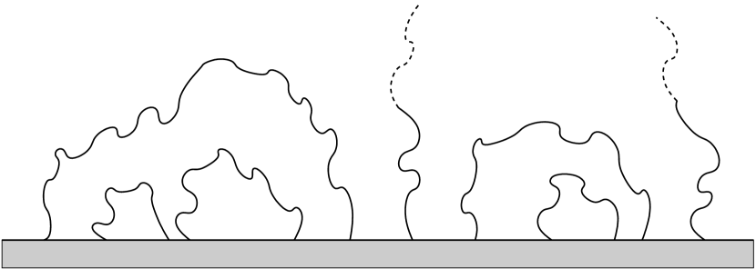
Figure 2: A topological configuration of the SLE traces is conjecturally related to the choice of integration contour for screening charges.

Consider $N$ simple curves in $\overline{\mathbb{H}}$ starting from $z_{1}<\cdots<z_{N}$ such that each curve either goes to infinity without intersecting any other, or is paired with another curve and doesn’t intersect any other curve exept at the common endpoint of its pair in $\mathbb{H}$ (and this endpoint is not on any other curve!). Let us denote the number of pairs by $L$. Observe that the configuration is fully determined if one knows which $z_{I}$ are left endpoints, meaning that the curve starting from $z_{I}$ is paired with $z_{J}>z_{I}$. Namely, to reconstruct the configuration proceed from the left. If $z_{1}$ is not a left endpoint the corresponding curve goes to $\infty$. If $z_{I}$, $I>1$ is not a left endpoint, there are two options. Either among $z_{1},\ldots,z_{I-1}$ there are left endpoints that don’t have a corresponding right endpoint among them. In this case $z_{I}$ must be the right endpoint of the righmost such left endpoint. If there are no such left endpoints, the curve at $z_{I}$ must go to infinity. This way of thinking leads to a bijection between configurations and walks $\omega:\{0,1,\ldots,N\}\rightarrow\mathbb{N}$ such that $\omega(0)=0$, $\omega(I)-\omega(I-1)=1$ if $z_{I}$ is not a right endpoint and $\omega(I)-\omega(I-1)=-1$ if $z_{I}$ is a right endpoint. The walks that end at $\omega(N)=N-2L$ correspond to $L$ pairs. The number of such walks is $(N+1-2L)\frac{N!}{L!(N-L+1)!}$. Let us denote the whole configuration by $p$.

Observe that we could have taken the integration contour in (19) to be such that integration contour of $w_{R}$ starts at the $R^{\textrm{th}}$ left endpoint and ends at the corresponding right endpoint (and the contours don’t intersect). Denote the corresponding screened vertex operator by $V^{(p)}$ and partition function by $Z^{(p)}=\big{<}v^{*}_{1,1+N-2L},V^{(p)}v_{1,1}\big{>}$. By Lemma 5.3 and obvious changes of variables we notice that $Z^{(p)}$ satisfies (b), (c) and (d) with homogeneity degree

$$\Delta=L+(\frac{1}{4}N(N-1)-NL+L(L-1))\alpha_{-}^{2}\textrm{ .}$$

Since $h_{1,r}=h(\frac{1-r}{2}\alpha_{-})=\frac{1-r}{2}+\frac{r^{2}-1}{4}\alpha_{-}^{2}$ we see that $\Delta=h_{1,1+N-2L}-Nh_{1,2}$ in accordance with the homogeneity degree expected of “pure geometry” with $N-2L$ curves going towards infinity.

If configuration $p$ is such that $z_{I}$ and $z_{J}$ are paired, then it is easy to see that as $|z_{I}-z_{J}|\rightarrow 0$

$$Z^{(p)}(z_{1},\ldots,z_{N})\sim(z_{I}-z_{J})^{\frac{\kappa-6}{\kappa}}Z^{(p^{\prime})}(z_{1},\ldots,z_{N})\textrm{ ,}$$

where $p^{\prime}$ is the configuration of $N-2$ curves and $L-1$ pairs which is obtained from $p$ by erasing the curve of $z_{I}$ and $z_{J}$. Furthermore, considering the behavior of the integrand we expect the asymptotic

$$Z^{(p)}\sim(z_{I}-z_{J})^{\frac{2}{\kappa}}$$

as $|z_{I}-z_{J}|\rightarrow 0$ for any two points $z_{I}$ and $z_{J}$ that are not paired. These asymptotics are what was in [6] argued for the “pure geometry” $p$, that is an SLE whose curves form the configuration $p$ almost surely.

We still remark that the vertex operator $V^{(p)}$ with integration contour $p$ is obtained from that of integration contour as in Figure 1, by braid group action on the screened vertex operators which has been studied in [18].

6.2 On M bius invariance

Consider an SLE whose state $M_{t}$ can be expressed as $G_{g_{t}}\Psi(X^{1}_{t},\ldots,Y^{M}_{t})\omega_{0}$ and $L_{0}\omega_{\infty}^{*}=0$ and $\big{<}L_{-1}\omega_{\infty}^{*},\Psi(x_{1},\ldots,y_{M})\omega_{0}\big{>}=0$ for all $x_{1},\ldots,y_{M}$. We then compute using the intertwining relation for $n=-1,0,1$ that $Z(\cdots)=\big{<}\omega_{\infty}^{*},\Psi(\cdots)\omega_{0}\big{>}$ satisfies the following

$$0\quad=\quad \big{<}\omega_{\infty}^{*},\;\Psi(x_{1},\ldots,y_{M})\;L_{n}\;\omega_{0}\big{>}$$

$$=\quad \big{<}\omega_{\infty}^{*},\;\Big{(}L_{n}\Psi-\big{(}\sum_{I}(x_{I}^{1+n}\frac{\partial}{\partial x_{I}}+(1+n)\delta_{x_{I}}x_{I}^{n})\big{)}\Psi$$

$$\qquad-\big{(}\sum_{K}(y_{K}^{1+n}\frac{\partial}{\partial y_{K}}+(1+n)\delta_{y_{K}}y_{K}^{n})\big{)}\Psi\Big{)}\;\omega_{0}\big{>}$$

$$=\quad -\Big{(}\sum_{I}(x_{I}^{1+n}\frac{\partial}{\partial x_{I}}+(1+n)\delta_{x_{I}}x_{I}^{n})$$

$$\qquad+\sum_{K}(y_{K}^{1+n}\frac{\partial}{\partial y_{K}}+(1+n)\delta_{y_{K}}y_{K}^{n})\Big{)}\;Z(x_{1},\ldots,y_{K})\textrm{ .}$$

The equations for $n=-1,0,1$ can be integrated to give the transformation properties of $Z$ under translations, dilatations and special conformal transformations

$$Z(x_{1}-\sigma,\ldots,y_{M}-\sigma)\; =\;Z(x_{1},\ldots,y_{M})$$

$$Z(e^{-\lambda}x_{1},\ldots,e^{-\lambda}y_{M})\; =\;e^{\lambda\delta_{x_{1}}}\cdots e^{\lambda\delta_{y_{M}}}\;Z(x_{1},\ldots,y_{M})$$

$$Z(\frac{x_{1}}{1+\rho x_{1}},\ldots,\frac{y_{M}}{1+\rho y_{M}})\; =\;(1+\rho x_{1})^{2\delta_{x_{1}}}\cdots(1+\rho y_{M})^{2\delta_{y_{M}}}\;Z(x_{1},\ldots,y_{M})$$

as long as $\rho$ is small enough so that $z\mapsto z/(1+\rho z)$ has not mapped any of the points to $\infty$. A general M bius transformation $\mu:\mathbb{H}\rightarrow\mathbb{H}$ that preserves the order of real points $x_{1},\ldots,x_{N},y_{1},\ldots,y_{M}$ can be written as a composition of special conformal transformation, dilatation and translation and the transformation properties are compactly

$$Z(\mu(x_{1}),\ldots,\mu(y_{M}))=\mu^{\prime}(x_{1})^{-\delta_{x_{1}}}\cdots\mu^{\prime}(y_{M})^{-\delta_{y_{M}}}\;Z(x_{1},\ldots,x_{N})\textrm{ .}$$ (20)

The following Proposition says that if $Z$ is M bius covariant in the sense of (20) then the SLE variant is M bius invariant up to a change in growth speeds. The assertion follows from a typical SLE computation and it can be found in [22] in a slightly different form.

Proposition 6.1.

Suppose the auxiliary function $Z$ of the SLE variant satisfies (20) for M bius transforms $\mu$ that preserve the order of $x_{1},\ldots,x_{N},y_{1},\ldots,y_{M}$. Choose $\mu_{t}:\mathbb{H}\rightarrow\mathbb{H}$ M bius such that

$$\tilde{g}_{t}=\mu_{t}\circ g_{t}\circ\mu^{-1}:\mathbb{H}\setminus\mu(K_{t})\rightarrow\mathbb{H}$$

is hydrodynamically normalized. Then $\tilde{g}_{t}$ describes an SLE variant with the same auxiliary function but different growth speeds, i.e.

$$\mathrm{d}\tilde{g}_{t}(z)\;=\; \sum_{I}\frac{2}{\tilde{g}_{t}(z)-\tilde{X}^{I}_{t}}\mathrm{d}\langle\tilde{A}^{I}\rangle_{t}\qquad\qquad\mathrm{d}\tilde{Y}_{t}\;=\;\sum_{I}\frac{2}{\tilde{Y}_{t}-\tilde{X}^{I}_{t}}\mathrm{d}\langle\tilde{A}^{I}\rangle_{t}$$

$$\mathrm{d}\tilde{X}^{I}_{t}\;=\; \sqrt{\kappa}\;\mathrm{d}\tilde{A}^{I}_{t}+\sum_{J\neq I}\frac{2}{\tilde{X}^{I}_{t}-\tilde{X}^{J}_{t}}\;\mathrm{d}\langle\tilde{A}^{J}\rangle_{t}$$

$$\;+\kappa\big{(}\partial_{x_{I}}\log Z)(\tilde{X}^{1}_{t},\ldots,\tilde{X}^{N}_{t})\big{)}\;\mathrm{d}\langle\tilde{A}^{I}\rangle_{t}\textrm{ ,}$$

where $\mathrm{d}\tilde{A}^{I}=\mu_{t}^{\prime}(X^{I}_{t})\;\mathrm{d}A^{I}_{t}$.

Remark 6.1.

Examples of Möbius invariant SLEs are e.g. SLE${}_{\kappa}(\rho_{1},\ldots,\rho_{M})$ such that $\sum_{K}\rho_{K}=\kappa-6$ as in [38] and certain pure geometries of multiple SLEs as we’ll soon see.

6.3 BRST cohomology and the structure of $\mathcal{M}$

Section 5 suggests that SLE state can often be constructed in charged Fock spaces. To study the Fock spaces and vertex operators Felder has introduced a method based on cohomology of BRST operators [19], see also [18, 8]. The “BRST charge” $Q_{m}$ is a $\mathfrak{vir}$-module homomorphism $F_{n,m}\rightarrow F_{n,-m}$. We refer the reader to [19] or [11] for the definition of it. Below we show how it can be applied to questions of SLE local martingales.

We will recall the Virasoro structure of $F_{n,m}$ in the generic case $\kappa\notin\mathbb{Q}$ and make remarks about the more complicated structure for $\kappa\in\mathbb{Q}$. Since the SLE states can in some cases be constructed in Fock spaces, this is a step towards resolving the structure of $\mathcal{M}$ because it must be a submodule of the contravariant module.

In the generic case $\kappa\notin\mathbb{Q}$ the Verma module $\mathcal{V}_{c,h_{n,m}}$, $n,m\geq 1$, contains one singular vector $\chi_{n,m}$ that generates a submodule isomorphic to $\mathcal{V}_{c,h_{n,m}+nm}$ which is irreducible (in the classification by Feigin and Fuchs this corresponds to case $\mathrm{II_{+}}$). The kernel $\mathrm{Ker}\;Q_{m}\subset F_{n,m}$ is a submodule and a closer study reveals that it is isomorphic to the irreducible highest weight $\mathfrak{vir}$-module $\mathrm{Ker}\;Q_{m}\cong\mathcal{H}_{n,m}=\mathcal{V}_{c,h_{n,m}}/\mathcal{U}(\mathfrak{vir})\chi_{n,m}$ of highest weight $h_{n,m}$.

A fact of great importance is that the BRST charge $Q$ commutes with vertex operators up to a factor. More precisely, if $V_{\underline{\alpha}}^{\Gamma;L,0}$ is a composition of vertex operators screened with $L$ charges $\alpha_{-}$ such that all $\alpha_{j}$’s are of the form $\alpha_{r_{j},s_{j}}$, $r_{j},s_{j}>0$ and $\sum_{j}\alpha_{j}=\alpha_{r,s}$, then $Q_{m+s-1-2L}\;V^{\Gamma;L,0}_{\underline{\alpha}}|_{F_{n,m}}=\mathrm{const.}\times V^{\Gamma^{\prime};s-L-1,0}_{\underline{\alpha}}|_{F_{n,-m}}\;Q_{m}$, where $\Gamma^{\prime}$ is another contour of screening with $s-L-1$ charges $\alpha_{-}$. In particular, screened vertex operators map the kernel of $Q$ to the kernel of $Q$. Since it can be checked that $v_{0}=v_{1,1}\in\mathrm{Ker}\;Q_{1}$, the states of multiple SLEs constructed in Section 5 by Coulomb gas method take values in the submodule $\mathrm{Ker}\;Q_{1+N-2L}\subset F_{1,1+N-2L}$. And since $\mathrm{Ker}\;Q_{1+N-2L}$ doesn’t contain the singular vector of $F_{1,1+N-2L}$ at level $1+N-2L$ we conclude that there is a nonzero vector at level $1+N-2L$ in $F^{*}_{1,1+N-2L}$ that annihilates $\mathrm{Ker}\;Q_{1+N-2L}$. But the SLE state takes values in the annihilated subspace so $\mathcal{M}$ has a null vector at level $1+N-2L$ (for generic $\kappa$ we readily conclude that the module $\mathcal{M}$ is irreducible). For example the null vector at level $2$ for ordinary chordal SLE (with $N=1$, $L=0$) can be understood in this way. A less well known case is multiple SLE with no curves to infinity i.e. $N=2L$. There is a vector at level $1$ in contravariant module that annihilates $\mathrm{Ker}\;Q_{1}$ so the considerations of Section 6.2 imply that such a multiple SLE is Möbius invariant.

In order not to give an overly simplified picture, let us point out that the non-generic case $\kappa\in\mathbb{Q}$ is quite involved. Write $\kappa/4=q/q^{\prime}$ such that $q,q^{\prime}\in\mathbb{N}$ have no common factors. Then we have $\alpha_{n,m}=\alpha_{n-q^{\prime},m-q}$ and we can view $Q_{q-m}:F_{n-q^{\prime},q-m}\rightarrow F_{n-q^{\prime},m-q}=F_{n,m}$. The BRST property is $Q_{m}Q_{q-m}=0$. The whole structure of Fock spaces as Virasoro modules (with all its exceptions) can be found in [16, 19, 8]. The charged Fock space $F_{1,m}$ contains infinitely many singular vectors $u_{i}$, $i=1,2,\ldots$ and to start with one would like to know whether they belong to the kernel of $Q_{m}$ or not. An SLE illustration of the complications is the example of SLE${}_{\kappa}(\kappa-6)$ in Section 4.6. This case can be viewed as a multiple SLE (with $N=2$, $L=1$) so that $\mathcal{M}$ must contain a null vector at level $1$. But at level $(q-1)(q^{\prime}-1)$ we can have either a null vector or a non-zero singular vector. It is worth noting that the latter has been so far unheard of in the SLE context and it immediately rules out the possibility of constructing the SLE state in a highest weight module for Virasoro algebra!

7 Conclusions

We have shown that local martingales for general variants of SLEs carry a representation of the Virasoro algebra. There exists a natural subrepresentation $\mathcal{M}$, whose interpretation was discussed. In the general case the structure of the module of local martingales has several properties that can not be seen in the simplest case of the chordal SLE towards infinity [3]. While some progress was made, the precise structure of $\mathcal{M}$ remains not completely resolved even for some of the most natural SLE variants.

Coulomb gas method of conformal field theory was used for constructing the SLE state explicitly in some particularly interesting cases. From the Coulomb gas method one obtains some results about the structure of the module as well. In particular for multiple SLEs, through the identification of $\mathcal{M}$ as a submodule in the contravariant module of $\mathrm{Ker}\;Q$, one gets the irreducibility of $\mathcal{M}$ for $\kappa$ generic and M bius invariance in certain cases. Further exploiting the BRST cohomology may be a promising approach to a better understanding of the Virasoro structure.

The Feigin-Fuchs integrals of the Coulomb gas give solutions to the system of differential equations needed to define multiple SLEs and the choice of contours of screening charges was argued to be transparently related to the conjecture of pure geometries.

The extensive discussion of interpretation should contribute to understanding more clearly the conformal field theoretic point of view to SLEs. Furthermore, the sole mechanism of constructing local martingales can turn out very useful as is illustrated for example by a novel approach to questions of SLE duality and chordal SLE reversibility in [29].

Acknowledgements. It is a pleasure to acknowledge that during the writing of this article I have benefited from interesting discussions with and useful remarks of Michel Bauer, Antti Kemppainen, Antti Kupiainen, Luigi Cantini and Krzysztof Gawȩdzki. A part of this work was done at the Department of Mathematics and Statistics at University of Helsinki and a part at the Service de Physique Théorique, CEA Saclay, and ENRAGE European Network MRTN-CT-2004-5616. The support of ANR-06-BLAN-0058-02 is gratefully acknowledged.

Appendix A Proof of Propositions 4.1 and 4.4

This Appendix contains a sketch of the computations proving Propositions 4.1 and 4.4. The computations are longish, but we will try to provide enough details for a dedicated reader to follow them without too much effort.

A.1 Lemmas for the computations

Certain kinds of terms will occur frequently in the computations so we write down some lemmas for these.

Lemma A.1.

For $p\in\mathbb{N}$ one has the following

$$\sum_{m\leq-2}\mathrm{Res}_{v}\; v^{-2-m}\big{(}\frac{1}{f(v)-r}\big{)}\frac{\partial}{\partial f_{m}}\Big{(}\big{(}\frac{1}{(f(w)-s)^{p}}\big{)}\Big{)}$$

$$=\; \Big{(}\frac{-p}{(f(w)-r)(f(w)-s)^{p+1}}\Big{)}$$ (21)

$$\sum_{m\leq-2}\mathrm{Res}_{v}\; v^{-2-m}\big{(}\frac{1}{f(v)-r}\big{)}\frac{\partial}{\partial f_{m}}\big{(}\frac{f^{\prime}(w)^{2}}{(f(w)-s)^{p}}\big{)}$$

$$=\; f^{\prime}(w)^{2}\Big{(}\frac{-p}{(f(w)-r)(f(w)-s)^{p+1}}+\frac{-2}{(f(w)-r)^{2}(f(w)-s)^{p}}\Big{)}$$ (22)

$$\sum_{m\leq-2}\mathrm{Res}_{v}\; v^{-2-m}\big{(}\frac{1}{f(v)-r}\big{)}\frac{\partial}{\partial f_{m}}\big{(}\frac{f^{\prime}(z)^{2}}{(f(w)-f(z))^{p}}\big{)}$$

$$=\; f^{\prime}(z)^{2}\Big{(}\big{(}\frac{1}{(f(w)-r)(f(z)-r)}\big{)}\frac{p}{(f(w)-f(z))^{p}}$$

$$\qquad+\frac{-2}{(f(z)-r)^{2}(f(w)-f(z))^{p}}\Big{)}\textrm{ ,}$$ (23)

where all the rational functions are expanded in $|f(v)|>|r|$, $|f(w)|>|s|$, $|f(w)|>|f(z)|$ and $|f(z)|>|r|$.

Proof.

These are direct computations. First observe that

$$\frac{\partial}{\partial f_{m}}\big{(}\frac{1}{(f(w)-s)^{p}}\big{)}\;=\; \frac{-p}{(f(w)-s)^{p+1}}w^{m+1}$$

$$\frac{\partial}{\partial f_{m}}\big{(}\frac{f^{\prime}(w)^{2}}{(f(w)-s)^{p}}\big{)}\;=\; \frac{2f^{\prime}(w)}{(f(w)-s)^{p}}(1+m)w^{m}-\frac{pf^{\prime}(w)^{2}}{(f(w)-s)^{p+1}}w^{m+1}$$

$$\frac{\partial}{\partial f_{m}}\big{(}\frac{f^{\prime}(z)^{2}}{(f(w)-f(z))^{p}}\big{)}\;=\; \frac{2f^{\prime}(z)}{(f(w)-f(z))^{p}}(1+m)z^{m}$$

$$-\frac{pf^{\prime}(z)^{2}}{(f(w)-f(z))^{p+1}}(w^{m+1}-z^{m+1})\textrm{ .}$$

The sums over $m$ in each case then consist of expansions of rational functions, whose expansion we will change as follows

$$\sum_{m\leq-2}v^{-2-m}w^{m+1}= \big{(}\frac{1}{w-v}\big{)}_{|w|>|v|}=\big{(}\frac{1}{w-v}\big{)}_{|v|>|w|}+\delta(w-v)$$

$$\sum_{m\leq-2}(1+m)v^{-2-m}w^{m}= \big{(}\frac{-1}{(w-v)^{2}}\big{)}_{|w|>|v|}=\big{(}\frac{-1}{(w-v)^{2}}\big{)}_{|v|>|w|}-\partial_{v}\delta(w-v)$$

Observe that after having changed the expansion the term involving rational functions contains no powers of $v$ greater than $-2$ so the residue of this part vanishes, e.g. in the case of (22)

$$\sum_{m\leq-2}\mathrm{Res}_{v}\;v^{-2-m}\big{(}\frac{1}{f(v)-r}\big{)}_{|f(v)|>|r|}\frac{\partial}{\partial f_{m}}\Big{(}f^{\prime}(w)^{2}\big{(}\frac{1}{(f(w)-s)^{p}}\big{)}_{|f(w)|>|s|}\Big{)}$$

$$=\; \mathrm{Res}_{v}\;\big{(}\frac{1}{f(v)-r}\big{)}_{|f(v)|>|r|}\Big{(}-p\frac{f^{\prime}(w)^{2}}{(f(w)-s)^{p+1}}\big{(}\frac{1}{w-v}+\delta(w-v)\big{)}$$

$$\qquad+2\frac{f^{\prime}(w)}{(f(w)-s)^{p}}\big{(}\frac{-1}{(w-v)^{2}}-\partial_{v}\delta(w-v)\big{)}\Big{)}_{|f(w)|>|s|,\;|v|>|w|}$$

$$=\; \Big{(}-p\frac{f^{\prime}(w)^{2}}{(f(w)-r)(f(w)-s)^{p+1}}+\frac{2f^{\prime}(w)}{(f(w)-s)^{p}}\partial_{w}\big{(}\frac{1}{f(w)-r}\big{)}\Big{)}_{|f(w)|>|r|,\;|f(w)|>|s|}$$

and the delta functions were easy to handle with an integration by parts. Computing the remaining derivative yields the result for (22) and this in fact contains also the computation needed for (21). For the last one, (23) we go ahead analogously

$$\sum_{m\leq-2}\mathrm{Res}_{v}\;v^{-2-m}\big{(}\frac{1}{f(v)-r}\big{)}_{|f(v)|>|r|}\frac{\partial}{\partial f_{m}}\big{(}\frac{f^{\prime}(z)^{2}}{(f(w)-f(z))^{p}}\big{)}_{|f(w)|>|s|}$$

$$=\; \mathrm{Res}_{v}\;\big{(}\frac{1}{f(v)-r}\big{)}_{|f(v)|>|r|}\Big{(}-\frac{2f^{\prime}(z)}{(f(w)-f(z))^{p}}\partial_{v}\delta(z-v)$$

$$\qquad-\frac{pf^{\prime}(z)^{2}}{(f(w)-f(z))^{p+1}}\big{(}\delta(w-v)-\delta(z-v)\big{)}\Big{)}$$

$$=\; \Big{(}+\frac{2f^{\prime}(z)}{(f(w)-f(z))^{p}}\partial_{z}\big{(}\frac{1}{f(z)-r}\big{)}-\frac{pf^{\prime}(z)^{2}}{(f(w)-f(z))^{p+1}}\big{(}\frac{1}{f(w)-r}-\frac{1}{f(z)-r}\big{)}\Big{)}\textrm{ ,}$$

where the expansions are in $|f(w)|>|r|$, $|f(z)|>|r|$ and $|f(w)|>|s|$. Use $(f(w)-r)^{-1}-(f(z)-r)^{-1}=(f(z)-f(w))\big{(}(f(w)-r)(f(z)-r)\big{)}^{-1}$ and compute the derivative $\partial_{z}(f(z)-r)^{-1}=-f^{\prime}(z)\,(f(z)-r)^{-2}$ to obtain the result (23). ∎

Lemma A.2.

One has

$$\sum_{m\leq-2}\mathrm{Res}_{v}\;v^{-2-m}\big{(}\frac{1}{f(v)-r}\big{)}_{|f(v)|>|r|}\frac{\partial}{\partial f_{m}}\big{(}Sf(w)\big{)}$$

$$=\; -6f^{\prime}(w)^{2}\big{(}\frac{1}{(f(w)-r)^{4}}\big{)}_{|f(w)|>|r|}\textrm{ .}$$

Proof.

The proof is similar to that of Lemma A.1. We start by computing

$$\frac{\partial}{\partial f_{m}}Sf(w)\;=\; \frac{\partial}{\partial f_{m}}\big{(}\frac{f^{\prime\prime\prime}(w)}{f^{\prime}(w)}-\frac{3}{2}\frac{f^{\prime\prime}(w)^{2}}{f^{\prime}(w)^{2}}\big{)}$$

$$=\; (m^{3}-m)w^{m-2}\frac{1}{f^{\prime}(w)}-3(m^{2}+m)w^{m-1}\frac{f^{\prime\prime}(w)}{f^{\prime}(w)^{2}}$$

$$\quad+(m+1)w^{m}\big{(}-\frac{f^{\prime\prime\prime}(w)}{f^{\prime}(w)^{2}}+3\frac{f^{\prime\prime}(w)^{2}}{f^{\prime}(w)^{3}}\big{)}\textrm{ .}$$

Then to change expansions we use

$$\sum_{m\leq-2}(m+1)v^{-2-m}w^{m}= \big{(}\frac{-1}{(w-v)^{2}}\big{)}_{|v|>|w|}-\partial_{v}\delta(w-v)$$

$$\sum_{m\leq-2}(m^{2}+m)v^{-2-m}w^{m-1}= \big{(}\frac{2}{(w-v)^{3}}\big{)}_{|v|>|w|}+\partial_{v}^{2}\delta(w-v)$$

$$\sum_{m\leq-2}(m^{3}-m)v^{-2-m}w^{m-2}= \big{(}\frac{-6}{(w-v)^{4}}\big{)}_{|v|>|w|}-\partial_{v}^{3}\delta(w-v)\textrm{ .}$$

It is already clear, just like in Lemma A.1, that only the delta function terms will contribute because the rest contains powers of $v$ not greater than $-2$. Thus $\sum_{m}\mathrm{Res}_{v}\;(f(v)-r)^{-1}v^{-2-m}\frac{\partial}{\partial f_{m}}Sf(w)$ can be written as

$$\Big{(}\big{(}-\frac{f^{\prime\prime\prime}(w)}{f^{\prime}(w)^{2}}+3\frac{f^{\prime\prime}(w)^{2}}{f^{\prime}(w)^{3}}\big{)}\partial_{w}-3\frac{f^{\prime\prime}(w)}{f^{\prime}(w)^{2}}\partial_{w}^{2}+\frac{1}{f^{\prime}(w)}\partial_{w}^{3}\Big{)}\;\big{(}\frac{1}{f(w)-r}\big{)}_{|f(w)|>|r|}\textrm{ .}$$

Now we substitute

$$\partial_{w}\big{(}\frac{1}{f(w)-r}\big{)}= \frac{-f^{\prime}(w)}{(f(w)-r)^{2}}$$

$$\partial_{w}^{2}\big{(}\frac{1}{f(w)-r}\big{)}= \frac{-f^{\prime\prime}(w)}{(f(w)-r)^{2}}+\frac{2f^{\prime}(w)^{2}}{(f(w)-r)^{3}}$$

$$\partial_{w}^{3}\big{(}\frac{1}{f(w)-r}\big{)}= \frac{-f^{\prime\prime\prime}(w)}{(f(w)-r)^{2}}+\frac{6f^{\prime\prime}(w)f^{\prime}(w)}{(f(w)-r)^{3}}+\frac{-6f^{\prime}(w)^{3}}{(f(w)-r)^{4}}$$

to obtain the asserted result. ∎

A.2 Proof of Proposition 4.1

We’ll now get started with the computation of $[\mathcal{L}_{n},\mathcal{T}(\zeta)]$. The “driving processes” $x_{I}$ and “passive points” $y_{K}$ play the same role in $\mathcal{T}(\zeta)$ so we simplify the notation by relabeling the $y_{K}$ as $x_{N+K}$. Furthermore we split $\mathcal{T}(\zeta)$ and $\mathcal{L}_{n}$ into parts as follows

$$\mathcal{T}(\zeta)\;=\; \mathcal{T}^{\partial f}(\zeta)+\mathcal{T}^{\partial x}(\zeta)+\mathcal{T}^{c}(\zeta)+\mathcal{T}^{h}(\zeta)\qquad\textrm{, where}$$

$$\mathcal{T}^{\partial f}(\zeta)\;=\; -\sum_{l\leq-2}\zeta^{-4}f^{\prime}(1/\zeta)^{2}\mathrm{Res}_{w}\;\big{(}\frac{w^{-2-l}}{f(w)-f(1/\zeta)}\big{)}_{|f(w)|>|f(1/\zeta)|}\;\frac{\partial}{\partial f_{l}}$$

$$\mathcal{T}^{\partial x}(\zeta)\;=\; \sum_{K=1}^{N+M}\zeta^{-4}f^{\prime}(1/\zeta)^{2}\big{(}\frac{1}{f(1/\zeta)-x_{K}}\big{)}_{|f(1/\zeta)|>|x_{K}|}\;\frac{\partial}{\partial x_{K}}$$

$$\mathcal{T}^{c}(\zeta)\;=\; \frac{c}{12}\zeta^{-4}Sf(1/\zeta)$$

$$\mathcal{T}^{h}(\zeta)\;=\; \sum_{K=1}^{N+M}\zeta^{-4}f^{\prime}(1/\zeta)^{2}\big{(}\frac{\delta_{x_{K}}}{(f(1/\zeta)-x_{K})^{2}}\big{)}_{|f(1/\zeta)|>|x_{K}|}\textrm{ ,}$$

and similarly $\mathcal{L}_{n}=\mathrm{Res}_{u}\;u^{-3-n}\mathcal{T}(u^{-1})=\mathcal{L}^{\partial f}_{n}+\mathcal{L}^{\partial y}_{n}+\mathcal{L}^{c}_{n}+\mathcal{L}^{h}_{n}$.

We will do the computation in four steps, gradually working through special cases and finally achieving the full result. The intermediate results can sometimes be very useful, too.

Step I: $\mathcal{T}^{\partial f}$

Let us first compute the part of the commutator in the simplest case $c=0$, $N=M=0$, in which $\mathcal{T}$ contains only the $\mathcal{T}^{\partial f}$ term. We compute

$$[\mathcal{L}^{\partial f}_{n},\mathcal{T}^{\partial f}]$$

$$=\; \sum_{l\leq-2}\mathrm{Res}_{z}\;\mathrm{Res}_{w}\;\mathrm{Res}_{u}\;\Big{\{}\frac{u^{1-n}f^{\prime}(u)^{2}}{f(z)-f(u)}\sum_{k\leq-2}z^{-2-k}\frac{\partial}{\partial f_{k}}\big{(}\zeta^{-4}\frac{f^{\prime}(1/\zeta)^{2}w^{-2-l}}{f(w)-f(1/\zeta)}\big{)}$$

$$\quad-\zeta^{-4}\frac{f^{\prime}(1/\zeta)^{2}}{f(w)-f(1/\zeta)}\sum_{k\leq-2}w^{-2-k}\frac{\partial}{\partial f_{k}}\big{(}\frac{u^{1-n}f^{\prime}(u)^{2}z^{-2-l}}{f(z)-f(u)}\big{)}\Big{\}}\;\frac{\partial}{\partial f_{l}}\textrm{ ,}$$

where the expansions of rational functions are in $|f(w)|>|f(1/\zeta)|$, $|f(z)|>|f(u)|$. We now apply to both terms Lemma A.1 (23) to write this as

$$\sum_{l\leq-2}\mathrm{Res}_{u}\;\Big{\{}\mathrm{Res}_{w}\;w^{-2-l}\Big{(}\frac{u^{1-n}f^{\prime}(u)^{2}\zeta^{-4}f^{\prime}(1/\zeta)^{2}\big{(}f(1/\zeta)+f(u)-2f(w)\big{)}}{(f(w)-f(1/\zeta))(f(w)-f(u))(f(1/\zeta)-f(u))^{2}}\Big{)}_{|f(1/\zeta)|>|f(u)|}$$

$$-\mathrm{Res}_{z}\;z^{-2-l}\frac{u^{1-n}f^{\prime}(u)^{2}\zeta^{-4}f^{\prime}(1/\zeta)^{2}\big{(}f(1/\zeta)+f(u)-2f(z)\big{)}}{(f(z)-f(1/\zeta))(f(z)-f(u))(f(1/\zeta)-f(u))^{2}}\Big{)}_{|f(u)|>|f(1/\zeta)|}\Big{\}}\frac{\partial}{\partial f_{l}}\textrm{ .}$$

We rename the dummy variable $z$ as $w$ and observe that the rational functions would cancel if they were expanded in the same region. So we will change the expansion of the former. To do this, we note that (10) can be used to show

$$\big{(}\frac{f^{\prime}(\rho)}{f(u)-f(\rho)}\big{)}_{|f(u)|>|f(\rho)|}-\big{(}\frac{f^{\prime}(\rho)}{f(u)-f(\rho)}\big{)}_{|f(\rho)|>|f(u)|}=\delta(u-\rho)\textrm{ .}$$

With a substitution $\rho=1/\zeta$ and a derivative w.r.t. $u$ we obtain

$$-\big{(}\frac{f^{\prime}(u)f^{\prime}(\rho)}{(f(u)-f(1/\zeta))^{2}}\big{)}_{|f(u)|>|f(1/\zeta)|} +\big{(}\frac{f^{\prime}(u)f^{\prime}(\rho)}{(f(u)-f(1/\zeta))^{2}}\big{)}_{|f(1/\zeta)|>|f(u)|}$$

$$\;=\; \partial_{u}\delta(u-1/\zeta)\textrm{ .}$$

Taking the residue will therefore be easily treated as soon as we have computed

$$\partial_{u}\Big{(}\frac{u^{1-n}f^{\prime}(u)\big{(}f(1/\zeta)+f(u)-2f(w)\big{)}}{(f(w)-f(u))}\Big{)}\Big{|}_{u=1/\zeta}$$

$$=\; \Big{(}-2\big{(}(1-n)\zeta^{n}f^{\prime}(1/\zeta)+\zeta^{n-1}f^{\prime\prime}(1/\zeta)\big{)}-\zeta^{n-1}\frac{f^{\prime}(1/\zeta)^{2}}{(f(w)-f(1/\zeta))}\Big{)}$$

which is needed when integrating by parts. The result for $[\mathcal{L}^{\partial f}_{n},\mathcal{T}^{\partial f}(\zeta)]$ is

$$\cdots\;=\; -\sum_{l\leq-2}\mathrm{Res}_{w}\;w^{-2-l}\big{(}\frac{\zeta^{-4}f^{\prime}(1/\zeta)}{(f(w)-f(1/\zeta))}\big{)}\Big{(}-\zeta^{n-1}\frac{f^{\prime}(1/\zeta)^{2}}{(f(w)-f(1/\zeta))}$$

$$\qquad-2\big{(}(1-n)\zeta^{n}f^{\prime}(1/\zeta)+\zeta^{n-1}f^{\prime\prime}(1/\zeta)\big{)}\Big{)}\;\frac{\partial}{\partial f_{l}}$$

$$=\; \sum_{l\leq-2}\mathrm{Res}_{w}\;w^{-2-l}\big{(}\frac{1}{(f(w)-f(1/\zeta))}\big{)}\Big{(}2(1-n)\zeta^{n-4}\frac{f^{\prime}(1/\zeta)^{2}}{(f(w)-f(1/\zeta))^{2}}$$

$$\quad+2\zeta^{n-5}\frac{f^{\prime\prime}(1/\zeta)f^{\prime}(1/\zeta)}{(f(w)-f(1/\zeta))^{2}}+\zeta^{n-5}\frac{f^{\prime}(1/\zeta)^{3}}{(f(w)-f(1/\zeta))^{2}}\Big{)}\;\frac{\partial}{\partial f_{l}}\textrm{ .}$$

But when we compare this and

$$\partial_{\zeta}\big{(}-\zeta^{-4}\frac{f^{\prime}(1/\zeta)^{2}}{f(w)-f(1/\zeta)}\big{)}$$

$$=\; 4\zeta^{-5}\frac{f^{\prime}(1/\zeta)^{2})}{f(w)-f(1/\zeta)}+2\zeta^{-6}\frac{f^{\prime\prime}(1/\zeta)f^{\prime}(1/\zeta)}{f(w)-f(1/\zeta)}+\zeta^{-6}\frac{f^{\prime}(1/\zeta)^{3}}{(f(w)-f(1/\zeta))^{2}}$$

we get the desired result

$$[\mathcal{L}^{\partial f}_{n},\mathcal{T}^{\partial f}(\zeta)]\;=\;(1+n)\zeta^{n}\big{(}2\mathcal{T}^{\partial f}(\zeta)\big{)}+\zeta^{1+n}\big{(}\partial_{\zeta}\mathcal{T}^{\partial f}(\zeta)\big{)}\textrm{ ,}$$

which also means that the operators $\mathcal{L}^{\partial f}_{n}$ satisfy the Witt algebra

$$[\mathcal{L}^{\partial f}_{n},\mathcal{L}^{\partial f}_{m}]=(n-m)\mathcal{L}^{\partial f}_{n+m}\textrm{ .}$$

Step II: $\mathcal{T}^{\partial f}+\mathcal{T}^{c}$

Next consider terms involving the central charge $c$ in the commutator $[\mathcal{L}_{n},\mathcal{T}(\zeta)]$. These are

$$\mathcal{L}^{\partial f}_{n}\mathcal{T}^{c}(\zeta)-\mathcal{T}^{\partial f}\mathcal{L}^{c}_{n}$$

$$=\; -\frac{c}{12}\mathrm{Res}_{u}\;\mathrm{Res}_{z}\;\sum_{l\leq-2}\Big{(}\frac{u^{1-n}f^{\prime}(u)^{2}z^{-2-l}}{f(z)-f(u)}\;\frac{\partial}{\partial f_{l}}Sf(1/\zeta)\zeta^{-4}$$

$$\qquad-\frac{\zeta^{-4}f^{\prime}(1/\zeta)^{2}z^{-2-l}}{f(z)-f(1/\zeta)}\;\frac{\partial}{\partial f_{l}}Sf(u)u^{1-n}\Big{)}\textrm{ .}$$

We apply Lemma A.2 to both terms and the above simplifies to

$$\frac{c}{2}\;\mathrm{Res}_{u}\;u^{1-n}f^{\prime}(u)^{2}\zeta^{-4}f^{\prime}(1/\zeta)^{2}\Big{(}\big{(}\frac{1}{(f(1/\zeta)-f(u))^{4}}\big{)}_{|f(1/\zeta)|>|f(u)|}$$

$$\qquad-\big{(}\frac{1}{(f(1/\zeta)-f(u))^{4}}\big{)}_{|f(1/\zeta)|>|f(u)|}\Big{)}\textrm{ .}$$

Thus we only have the contribution from changing the expansions, the “residue at $u=1/\zeta$”. The straightforward evaluation of this gives

$$\frac{c}{12}\Big{(}\zeta^{n-2}(n^{3}-n)-3\zeta^{n-5}\frac{f^{\prime\prime}(1/\zeta)^{3}}{f^{\prime}(1/\zeta)^{3}}-3(n-1)\zeta^{n-4}\frac{f^{\prime\prime}(1/\zeta)^{2}}{f^{\prime}(1/\zeta)^{2}}$$

$$+4\zeta^{n-5}\frac{f^{\prime\prime}(1/\zeta)f^{\prime\prime\prime}(1/\zeta)}{f^{\prime}(1/\zeta)^{2}}+2(n-1)\zeta^{n-4}\frac{f^{\prime\prime\prime}(1/\zeta)}{f^{\prime}(1/\zeta)}-\zeta^{n-5}\frac{f^{\prime\prime\prime\prime}(1/\zeta)}{f^{\prime}(1/\zeta)}\Big{)}$$

$$=\; \frac{c}{12}\Big{(}\zeta^{n-2}(n^{3}-n)+(1+n)\zeta^{n}\;\big{(}2\zeta^{-4}Sf(1/\zeta)\big{)}+\zeta^{1+n}\;\partial_{\zeta}\big{(}\zeta^{-4}Sf(1/\zeta)\big{)}\Big{)}\textrm{ ,}$$

as it should. In other words, we have

$$[\mathcal{L}^{\partial f}_{n}+\mathcal{L}^{c}_{n},\mathcal{T}^{\partial f}(\zeta)+\mathcal{T}^{c}(\zeta)]$$

$$=\; \frac{c}{12}\zeta^{n-2}(n^{3}-n)+(1+n)\zeta^{n}\;2\big{(}\mathcal{T}^{\partial f}(\zeta)+\mathcal{T}^{c}(\zeta)\big{)}+\zeta^{1+n}\;\partial_{\zeta}\big{(}\mathcal{T}^{\partial f}(\zeta)+\mathcal{T}^{c}(\zeta)\big{)}$$

and thus $\mathcal{L}^{\partial f}_{n}+\mathcal{L}^{c}_{n}$ satisfy the Virasoro algebra

$$[(\mathcal{L}^{\partial f}_{n}+\mathcal{L}^{c}_{n}),(\mathcal{L}^{\partial f}_{m}+\mathcal{L}^{c}_{m})]$$

$$=\; (n-m)(\mathcal{L}^{\partial f}_{n+m}+\mathcal{L}^{c}_{n+m})+\frac{c}{12}(n^{3}-n)\delta_{n+m,0}\textrm{ .}$$

Step III: $\mathcal{T}^{\partial f}+\mathcal{T}^{c}+\mathcal{T}^{\partial y}$

The remaining task is to compute the terms involving the points $y_{K}$ and we will start with the special case of vanishing $\delta_{x_{I}}$.

Let us first aim at finding out what is $\mathcal{L}^{\partial x}_{n}+\mathcal{L}^{\partial f}_{n}$ acting on $\mathcal{T}^{\partial x}$. We use Lemma A.1 (22) to get

$$\mathrm{Res}_{u}\;u^{1-n}f^{\prime}(u)^{2}\Big{(}\sum_{K}\frac{1}{f(u)-x_{K}}\frac{\partial}{\partial x_{K}}$$

$$\qquad-\mathrm{Res}_{z}\;\sum_{l\leq-2}\frac{z^{-2-l}}{f(z)-f(u)}\frac{\partial}{\partial f_{l}}\Big{)}\;\frac{\zeta^{-4}f^{\prime}(1/\zeta)^{2}}{f(1/\zeta)-x_{J}}$$

$$=\; \mathrm{Res}_{u}\;u^{1-n}f^{\prime}(u)^{2}\zeta^{-4}f^{\prime}(1/\zeta)^{2}\Big{(}\frac{1}{(f(1/\zeta)-f(u))(f(1/\zeta)-x_{J})^{2}}$$

$$\qquad+\frac{2}{(f(1/\zeta)-f(u))^{2}(f(1/\zeta)-x_{J})}+\frac{1}{(f(u)-x_{J})(f(1/\zeta)-x_{J})^{2}}\Big{)}$$

$$=\; \mathrm{Res}_{u}\;u^{1-n}f^{\prime}(u)^{2}\zeta^{-4}f^{\prime}(1/\zeta)^{2}\Big{(}\frac{f(u)+f(1/\zeta)-2x_{J}}{(f(1/\zeta)-f(u))^{2}(f(u)-x_{J})(f(1/\zeta)-x_{J})}\Big{)}$$

expanded in $|f(1/\zeta)|>|f(u)|$. One does a completely analogous computation for $\mathcal{T}^{\partial x}+\mathcal{T}^{\partial f}$ acting on $\mathcal{L}^{\partial x}_{n}$ to yield a nice looking result

$$\big{(}\mathcal{L}^{\partial x}_{n}+\mathcal{L}^{\partial f}_{n}\big{)}\mathcal{T}^{\partial x}(\zeta)-\big{(}\mathcal{T}^{\partial x}(\zeta)+\mathcal{T}^{\partial f}(\zeta)\big{)}\mathcal{L}^{\partial x}_{n}$$

$$=\; \sum_{J}\mathrm{Res}_{u}\;u^{1-n}f^{\prime}(u)^{2}\zeta^{-4}f^{\prime}(1/\zeta)^{2}\Big{(}\frac{f(u)+f(1/\zeta)-2x_{J}}{(f(u)-x_{J})(f(1/\zeta)-x_{J})}\Big{)}$$

$$\qquad\Big{(}\big{(}\frac{1}{(f(1/\zeta)-f(u))^{2}}\big{)}_{|f(1/\zeta)|>|f(u)|}-\big{(}\frac{1}{(f(1/\zeta)-f(u))^{2}}\big{)}_{|f(u)|>|f(1/\zeta)|}\Big{)}\;\frac{\partial}{\partial x_{J}}\textrm{ .}$$

We’re again in a position to change the expansions to get the “residue at $u=1/\zeta$”. The formula for change of expansion was given in Step I. The integration by parts now essentially consists of computing

$$\partial_{u}\Big{(}\frac{u^{1-n}f^{\prime}(u)\big{(}f(u)+f(1/\zeta)-2x_{J}\big{)}}{(f(u)-x_{J})}\Big{)}\Big{|}_{u=1/\zeta}$$

$$=\; \Big{(}2\big{(}(1-n)\zeta^{n}f^{\prime}(1/\zeta)+\zeta^{n-1}f^{\prime\prime}(1/\zeta)\big{)}-\zeta^{n-1}\frac{f^{\prime}(1/\zeta)^{2}}{(f(1/\zeta)-x_{J})}\Big{)}\textrm{ .}$$

Now we can write

$$\big{(}\mathcal{L}^{\partial x}_{n}+\mathcal{L}^{\partial f}_{n}\big{)}\mathcal{T}^{\partial x}(\zeta)-\big{(}\mathcal{T}^{\partial x}(\zeta)+\mathcal{T}^{\partial f}(\zeta)\big{)}\mathcal{L}^{\partial x}_{n}$$

$$=\; -\sum_{J}\Big{(}\frac{\zeta^{-4}f^{\prime}(1/\zeta)}{(f(1/\zeta)-x_{J})}\Big{)}\Big{(}2\big{(}(1-n)\zeta^{n}f^{\prime}(1/\zeta)+\zeta^{n-1}f^{\prime\prime}(1/\zeta)\big{)}$$

$$\qquad-\zeta^{n-1}\frac{f^{\prime}(1/\zeta)^{2}}{(f(1/\zeta)-x_{J})}\Big{)}\;\frac{\partial}{\partial x_{J}}$$

$$=\; \sum_{J}\Big{(}-2(1-n)\zeta^{n-4}\frac{f^{\prime}(1/\zeta)^{2}}{f(1/\zeta)-x_{J}}-2\zeta^{n-5}\frac{f^{\prime\prime}(1/\zeta)f^{\prime}(1/\zeta)}{f(1/\zeta)-x_{J}}$$

$$\qquad+\zeta^{n-5}\frac{f^{\prime}(1/\zeta)^{3}}{(f(1/\zeta)-x_{J})^{2}}\Big{)}\;\frac{\partial}{\partial x_{J}}$$

and compare with

$$\partial_{\zeta}\Big{(}\zeta^{-4}\frac{f^{\prime}(1/\zeta)^{2}}{f(1/\zeta)-x_{J}}\Big{)}$$

$$=\; -4\zeta^{-5}\frac{f^{\prime}(1/\zeta)^{2}}{f(1/\zeta)-x_{J}}-2\zeta^{-6}\frac{f^{\prime\prime}(1/\zeta)f^{\prime}(1/\zeta)}{f(1/\zeta)-x_{J}}+\zeta^{-6}\frac{f^{\prime}(1/\zeta)^{3}}{(f(1/\zeta)-x_{J})^{2}}$$

to notice that

$$\big{(}\mathcal{L}^{\partial x}_{n}+\mathcal{L}^{\partial f}_{n}\big{)}\mathcal{T}^{\partial x}(\zeta)-\big{(}\mathcal{T}^{\partial x}(\zeta)+\mathcal{T}^{\partial f}(\zeta)\big{)}\mathcal{L}^{\partial x}_{n}$$

$$=\; (1+n)\zeta^{n}\big{(}2\mathcal{T}^{\partial x}(\zeta)\big{)}+\zeta^{1+n}\big{(}\partial_{\zeta}\mathcal{T}^{\partial x}(\zeta)\big{)}\textrm{ .}$$

Combining with Step I and Step II we have shown that

$$[\mathcal{L}^{\partial f}_{n}+\mathcal{L}^{c}_{n}+\mathcal{L}^{\partial x}_{n},\mathcal{T}^{\partial f}(\zeta)+\mathcal{T}^{c}(\zeta)+\mathcal{T}^{\partial x}(\zeta)]$$

$$=\; \frac{c}{12}\zeta^{n-2}(n^{3}-n)+(1+n)\zeta^{n}\;2\big{(}\mathcal{T}^{\partial f}(\zeta)+\mathcal{T}^{c}(\zeta)+\mathcal{T}^{\partial x}(\zeta)\big{)}$$

$$+\zeta^{1+n}\;\partial_{\zeta}\big{(}\mathcal{T}^{\partial f}(\zeta)+\mathcal{T}^{c}(\zeta)+\mathcal{T}^{\partial x}(\zeta)\big{)}$$

and again $\mathcal{L}^{\partial f}_{n}+\mathcal{L}^{c}_{n}+\mathcal{L}^{\partial y}_{n}$ satisfy the Virasoro algebra

$$[(\mathcal{L}^{\partial f}_{n}+\mathcal{L}^{c}_{n}+\mathcal{L}^{\partial x}_{n}),(\mathcal{L}^{\partial f}_{m}+\mathcal{L}^{c}_{m}+\mathcal{L}^{\partial x}_{m})]$$

$$=\; (n-m)(\mathcal{L}^{\partial f}_{n+m}+\mathcal{L}^{c}_{n+m}+\mathcal{L}^{\partial x}_{n+m})+\frac{c}{12}(n^{3}-n)\delta_{n+m,0}\textrm{ .}$$

Step IV: $\mathcal{T}^{\partial f}+\mathcal{T}^{c}+\mathcal{T}^{\partial y}+\mathcal{T}^{h}$

The last piece to take into account is $\mathcal{T}^{h}$, that is to allow nonvanishing $\delta_{x_{K}}$. Its treatment is very similar to Step III. We’d like to compute what is $\mathcal{L}^{\partial x}_{n}+\mathcal{L}^{\partial f}_{n}$ acting on $\mathcal{T}^{h}$ so we begin by using Lemma A.1 (22)

$$\mathrm{Res}_{u}\;u^{1-n}f^{\prime}(u)^{2}\Big{(}\sum_{K}\frac{1}{f(u)-x_{K}}\frac{\partial}{\partial x_{K}}$$

$$\qquad-\mathrm{Res}_{z}\;\sum_{l\leq-2}\frac{z^{-2-l}}{f(z)-f(u)}\frac{\partial}{\partial f_{l}}\Big{)}\;\frac{\delta_{x_{J}}\,\zeta^{-4}f^{\prime}(1/\zeta)^{2}}{(f(1/\zeta)-x_{J})^{2}}$$

$$=\; \mathrm{Res}_{u}\;u^{1-n}f^{\prime}(u)^{2}\zeta^{-4}f^{\prime}(1/\zeta)^{2}\Big{(}\frac{2\delta_{x_{J}}}{(f(1/\zeta)-f(u))(f(1/\zeta)-x_{J})^{3}}$$

$$\qquad+\frac{2\delta_{x_{J}}}{(f(1/\zeta)-f(u))^{2}(f(1/\zeta)-x_{J})^{2}}+\frac{2\delta_{x_{J}}}{(f(u)-x_{J})(f(1/\zeta)-x_{J})^{3}}\Big{)}$$

$$=\; \mathrm{Res}_{u}\;u^{1-n}f^{\prime}(u)^{2}\zeta^{-4}f^{\prime}(1/\zeta)^{2}\Big{(}\frac{2\delta_{x_{J}}}{(f(1/\zeta)-f(u))^{2}(f(1/\zeta)-x_{J})(f(u)-x_{J})}\Big{)}$$

expanded in $|f(1/\zeta)|>|f(u)|$. Do the same for $\mathcal{T}^{\partial x}+\mathcal{T}^{\partial f}$ acting on $\mathcal{L}^{h}_{n}$ and obtain

$$\big{(}\mathcal{L}^{\partial x}_{n}+\mathcal{L}^{\partial f}_{n}\big{)}\mathcal{T}^{h}(\zeta)-\big{(}\mathcal{T}^{\partial x}(\zeta)+\mathcal{T}^{\partial f}(\zeta)\big{)}\mathcal{L}^{h}_{n}$$

$$=\; \sum_{J}\mathrm{Res}_{u}\;u^{1-n}f^{\prime}(u)^{2}\zeta^{-4}f^{\prime}(1/\zeta)^{2}\Big{(}\frac{2\delta_{x_{J}}}{(f(1/\zeta)-x_{J})(f(u)-x_{J})}\Big{)}$$

$$\qquad\Big{(}\big{(}\frac{1}{(f(1/\zeta)-f(u))^{2}}\big{)}_{|(f(1/\zeta)|>|(f(u)|}-\big{(}\frac{1}{(f(1/\zeta)-f(u))^{2}}\big{)}_{|f(u)|>|(f(1/\zeta)|}\Big{)}\textrm{ .}$$

After changing the expansion with the formula found in Step I we need the following

$$\partial_{u}\Big{(}\frac{u^{1-n}f^{\prime}(u)}{(f(u)-x_{J})}\Big{)}\Big{|}_{u=1/\zeta}$$

$$=\; (1-n)\zeta^{n}\frac{f^{\prime}(1/\zeta)}{(f(u)-x_{J})}+\zeta^{n-1}\frac{f^{\prime\prime}(1/\zeta)}{(f(u)-x_{J})}-\zeta^{n-1}\frac{f^{\prime}(1/\zeta)^{2}}{(f(u)-x_{J})^{2}}$$

for integration by parts. The result can now be written as

$$\big{(}\mathcal{L}^{\partial x}_{n}+\mathcal{L}^{\partial f}_{n}\big{)}\mathcal{T}^{h}(\zeta)-\big{(}\mathcal{T}^{\partial x}(\zeta)+\mathcal{T}^{\partial f}(\zeta)\big{)}\mathcal{L}^{h}_{n}$$

$$=\; -\sum_{J}\frac{2\delta_{x_{J}}\zeta^{-4}f^{\prime}(1/\zeta)}{(f(1/\zeta)-x_{J})}\Big{(}\frac{(1-n)\zeta^{n}f^{\prime}(1/\zeta)}{(f(u)-x_{J})}+\frac{\zeta^{n-1}f^{\prime\prime}(1/\zeta)}{(f(u)-x_{J})}-\frac{\zeta^{n-1}f^{\prime}(1/\zeta)^{2}}{(f(u)-x_{J})^{2}}\Big{)}$$

$$=\; \sum_{J}2\delta_{x_{J}}\Big{(}-\frac{(1-n)\zeta^{n-4}f^{\prime}(1/\zeta)^{2}}{(f(u)-x_{J})^{2}}-\frac{\zeta^{n-5}f^{\prime\prime}(1/\zeta)f^{\prime}(1/\zeta)}{(f(u)-x_{J})^{2}}+\frac{\zeta^{n-5}f^{\prime}(1/\zeta)^{3}}{(f(u)-x_{J})^{3}}\Big{)}$$

and comparison with

$$\partial_{\zeta}\Big{(}\zeta^{-4}\frac{f^{\prime}(1/\zeta)^{2}}{(f(1/\zeta)-x_{J})^{2}}\Big{)}$$

$$=\; -4\zeta^{-5}\frac{f^{\prime}(1/\zeta)^{2}}{(f(1/\zeta)-x_{J})^{2}}-2\zeta^{-6}\frac{f^{\prime\prime}(1/\zeta)f^{\prime}(1/\zeta)}{(f(1/\zeta)-x_{J})^{2}}+2\zeta^{-6}\frac{f^{\prime}(1/\zeta)^{3}}{(f(1/\zeta)-x_{J})^{3}}$$

yields the anticipated result

$$\big{(}\mathcal{L}^{\partial x}_{n}+\mathcal{L}^{\partial f}_{n}\big{)}\mathcal{T}^{h}(\zeta)-\big{(}\mathcal{T}^{\partial x}(\zeta)+\mathcal{T}^{\partial f}(\zeta)\big{)}\mathcal{L}^{h}_{n}$$

$$=\; (1+n)\zeta^{n}\big{(}2\mathcal{T}^{h}(\zeta)\big{)}+\zeta^{1+n}\big{(}\partial_{\zeta}\mathcal{T}^{h}(\zeta)\big{)}\textrm{ .}$$

This concludes the proof of Proposition 4.1 since together with results of Steps I-III it means

$$[\mathcal{L}_{n},\mathcal{T}(\zeta)]\;=\;(1+n)\zeta^{n}\big{(}2\mathcal{T}(\zeta)\big{)}+\zeta^{1+n}\big{(}\partial_{\zeta}\mathcal{T}(\zeta)\big{)}$$

which in turn is equivalent to the $\mathcal{L}_{n}$ forming a representation of the Virasoro algebra

$$[\mathcal{L}_{n},\mathcal{L}_{m}]\;=\;(n-m)\mathcal{L}_{n+m}+\frac{c}{12}(n^{3}-n)\delta_{n+m,0}\textrm{ . }\quad\square$$

A.3 Proof of Proposition 4.4

This appendix contains the computations proving Proposition 4.4. We will continue to denote $y_{K}$ by $x_{N+K}$ for simplicity of notation. Thus we will use for $I=1,\ldots,N$ (for the variables corresponding to the actual driving processes)

$$\mathcal{A}_{I} = \frac{\kappa_{I}}{2}\frac{\partial^{2}}{\partial x_{I}^{2}}+\sum_{J\neq I}\big{(}\frac{2}{x_{J}-x_{I}}\frac{\partial}{\partial x_{J}}-\frac{2h_{x_{J}}}{(x_{J}-x_{I})^{2}}\big{)}$$

$$+2\sum_{m\leq-2}\mathrm{Res}_{v}\;v^{-2-m}\big{(}\frac{1}{f(v)-x_{I}}\big{)}_{|f(v)|\;\mathrm{large}}\;\frac{\partial}{\partial f_{m}}\textrm{ ,}$$

where the first line corresponds to the operator $\mathcal{D}_{I}$ of null field equation (b). One should observe that for the statement about $[\mathcal{T}(\zeta),\mathcal{A}_{I}]$ it will only be necessary to require $c=\frac{(3\kappa_{I}-8)(6-\kappa_{I})}{2\kappa_{I}}$ and $\delta_{x_{I}}=h_{x_{I}}=\frac{6-\kappa_{I}}{2\kappa_{I}}$ but $\delta_{x_{J}}=h_{x_{J}}$ for $J\neq I$ can take any values (in particular this is the case of the passive points $y_{K}$ now labeled as $x_{N+K}$).

Let’s start by applying Lemma A.1 (21) & (23) to the part

$$[\mathcal{T}^{\partial f}(\zeta),2\,\sum_{m\leq-2}\mathrm{Res}_{v}\;\frac{v^{-2-m}}{f(v)-x_{I}}\frac{\partial}{\partial f_{m}}]$$

$$=\; -\sum_{l\leq-2}\mathrm{Res}_{w}\;\zeta^{-4}\frac{f^{\prime}(1/\zeta)^{2}w^{-2-l}}{f(w)-f(1/\zeta)}\sum_{m\leq-2}\frac{\partial}{\partial f_{l}}\Big{(}\mathrm{Res}_{v}\;\frac{2v^{-2-m}}{f(v)-x_{I}}\Big{)}\frac{\partial}{\partial f_{m}}$$

$$-\sum_{m\leq-2}\mathrm{Res}_{v}\;\frac{2v^{-2-m}}{f(v)-x_{I}}\sum_{l\leq-2}\frac{\partial}{\partial f_{m}}\Big{(}-\zeta^{-4}\frac{f^{\prime}(1/\zeta)^{2}w^{-2-l}}{f(w)-f(1/\zeta)}\Big{)}\frac{\partial}{\partial f_{l}}$$

$$=\; 2\sum_{m\leq-2}\mathrm{Res}_{v}\;\zeta^{-4}\frac{f^{\prime}(1/\zeta)^{2}}{f(v)-f(1/\zeta)}\frac{v^{-2-m}}{(f(v)-x_{I})^{2}}\;\frac{\partial}{\partial f_{m}}$$

$$+2\sum_{l\leq-2}\mathrm{Res}_{w}\;\zeta^{-4}\frac{f^{\prime}(1/\zeta)^{2}w^{-2-l}}{f(w)-f(1/\zeta)}\Big{(}\frac{1}{(f(w)-x_{I})(f(1/\zeta)-x_{I})}$$

$$\qquad+\frac{-2}{(f(1/\zeta)-x_{I})^{2}}\Big{)}\;\frac{\partial}{\partial f_{l}}\textrm{ .}$$

We’ll rename the dummy variables $w$ as $v$ and $l$ as $m$ to combine the two terms. In addition we take into account the term $\mathcal{T}^{\partial x}$ acting on $\sum_{m}\mathrm{Res}_{v}\;\frac{2v^{-2-m}}{f(v)-x_{I}}\frac{\partial}{\partial f_{m}}$, that is

$$2\sum_{m\leq-2}\mathrm{Res}_{v}\;\zeta^{-4}\frac{f^{\prime}(1/\zeta)^{2}}{f(1/\zeta)-x_{I}}\frac{v^{-2-m}}{(f(v)-x_{I})^{2}}\;\frac{\partial}{\partial f_{m}}\textrm{ .}$$

The sum of the terms considered above is

$$-4\,\zeta^{-4}\frac{f^{\prime}(1/\zeta)^{2}}{(f(1/\zeta)-x_{I})^{2}}\sum_{m\leq-2}\mathrm{Res}_{v}\;\frac{v^{-2-m}}{f(v)-x_{I}}\frac{\partial}{\partial f_{m}}\textrm{ .}$$ (24)

The only term that will contain the central charge $c$ comes from the action of $\sum_{m}\mathrm{Res}_{v}\;\frac{2v^{-2-m}}{f(v)-x_{I}}\frac{\partial}{\partial f_{m}}$ on $\mathcal{T}^{c}$, and it is readily computed with the help of Lemma A.2

$$[\mathcal{T}^{c}(\zeta),2\,\sum_{m\leq-2}\mathrm{Res}_{v}\;\frac{v^{-2-m}}{f(v)-x_{I}}\frac{\partial}{\partial f_{m}}]$$

$$=\; -2\,\sum_{m\leq-2}\mathrm{Res}_{v}\;\frac{v^{-2-m}}{f(v)-x_{I}}\frac{\partial}{\partial f_{m}}\Big{(}\frac{c}{12}\zeta^{-4}Sf(1/\zeta)\Big{)}$$

$$=\; c\;\zeta^{-4}\frac{f^{\prime}(1/\zeta)^{2}}{(f(1/\zeta)-x_{I})^{4}}\textrm{ .}$$ (25)

Next, let’s see what are the contributions of $\sum_{m}\mathrm{Res}_{v}\;\frac{2v^{-2-m}}{f(v)-x_{I}}\frac{\partial}{\partial f_{m}}$ acting on $\mathcal{T}^{\partial x}$ and $\mathcal{T}^{h}$. In both cases Lemma A.1 (22) will be used. The former is

$$-2\,\sum_{m\leq-2}\mathrm{Res}_{v}\;\frac{v^{-2-m}}{f(v)-x_{I}}\sum_{J}\frac{\partial}{\partial f_{m}}\Big{(}\zeta^{-4}\frac{f^{\prime}(1/\zeta)^{2}}{f(1/\zeta)-x_{J}}\Big{)}\;\frac{\partial}{\partial x_{J}}$$

$$=\; \sum_{J}\Big{(}\frac{2\zeta^{-4}f^{\prime}(1/\zeta)^{2}}{(f(1/\zeta)-x_{I})(f(1/\zeta)-x_{J})^{2}}+\frac{4\zeta^{-4}f^{\prime}(1/\zeta)^{2}}{(f(1/\zeta)-x_{I})^{2}(f(1/\zeta)-x_{J})}\Big{)}\;\frac{\partial}{\partial x_{J}}$$

and the latter

$$-2\,\sum_{m\leq-2}\mathrm{Res}_{v}\;\frac{v^{-2-m}}{f(v)-x_{I}}\sum_{J}\frac{\partial}{\partial f_{m}}\Big{(}\zeta^{-4}\frac{\delta_{x_{J}}f^{\prime}(1/\zeta)^{2}}{f(1/\zeta)-x_{J}}\Big{)}$$

$$=\; \sum_{J}\Big{(}\frac{4\delta_{x_{J}}\zeta^{-4}f^{\prime}(1/\zeta)^{2}}{(f(1/\zeta)-x_{I})(f(1/\zeta)-x_{J})^{3}}+\frac{4\delta_{x_{J}}\zeta^{-4}f^{\prime}(1/\zeta)^{2}}{(f(1/\zeta)-x_{I})^{2}(f(1/\zeta)-x_{J})^{2}}\Big{)}\textrm{ .}$$

What remains is the commutator of $\mathcal{T}$ with $\mathcal{D}_{I}$. This is

$$[\mathcal{T}^{\partial y}(\zeta)+\mathcal{T}^{h}(\zeta)\,,\,\mathcal{D}_{I}]$$

$$=\; \zeta^{-4}f^{\prime}(1/\zeta)^{2}\Big{\{}-\frac{\kappa_{I}}{2}\frac{2}{(f(1/\zeta)-x_{I})^{2}}\frac{\partial^{2}}{\partial x_{I}^{2}}-\frac{\kappa_{I}}{2}\frac{6\delta_{x_{I}}}{(f(1/\zeta)-x_{I})^{4}}$$

$$\quad-\kappa_{I}\big{(}\frac{1}{(f(1/\zeta)-x_{I})^{3}}+\frac{2\delta_{x_{I}}}{(f(1/\zeta)-x_{I})^{3}}\big{)}\frac{\partial}{\partial x_{I}}$$

$$\quad-\sum_{J\neq I}\frac{2}{x_{J}-x_{I}}\Big{(}\frac{1}{(f(1/\zeta)-x_{J})^{2}}\frac{\partial}{\partial x_{J}}+\frac{2\delta_{x_{J}}}{(f(1/\zeta)-x_{J})^{3}}\Big{)}$$

$$\quad+\sum_{J\neq I}\frac{x_{J}-x_{I}}{(f(1/\zeta)-x_{J})(f(1/\zeta)-x_{I})}\Big{(}\frac{-2}{(x_{J}-x_{I})^{2}}\frac{\partial}{\partial x_{J}}+\frac{4h_{x_{J}}}{(x_{J}-x_{I})^{3}}\Big{)}\Big{\}}\textrm{ .}$$

We will collect the different terms from $[\mathcal{T},\mathcal{D}_{I}]$ and $\sum_{m}\mathrm{Res}_{v}\;\frac{2v^{-2-m}}{f(v)-x_{I}}\frac{\partial}{\partial f_{m}}$ acting on $\mathcal{T}^{\partial x}$ and $\mathcal{T}^{h}$. The terms with derivatives with respect to $x_{I}$ are

$$-\kappa_{I}\;\zeta^{-4}\frac{f^{\prime}(1/\zeta)^{2}}{(f(1/\zeta)-x_{I})^{2}}\frac{\partial^{2}}{\partial x_{I}^{2}}+\zeta^{-4}\frac{f^{\prime}(1/\zeta)^{2}(6-\kappa_{I}-2\kappa_{I}\delta_{x_{I}})}{(f(1/\zeta)-x_{I})^{3}}\frac{\partial}{\partial x_{I}}$$ (26)

whereas the terms with derivatives with respect to $x_{J}$, $J\neq I$, are

$$-4\;\zeta^{-4}\frac{f^{\prime}(1/\zeta)^{2}}{(f(1/\zeta)-x_{I})^{2}}\;\sum_{J\neq I}\frac{1}{x_{J}-x_{I}}\;\frac{\partial}{\partial x_{J}}\textrm{ .}$$ (27)

We write the pure multiplication operator terms slightly suggestively separating parts proportional to $(\delta_{x_{J}}-h_{x_{J}})$

$$\zeta^{-4}\frac{f^{\prime}(1/\zeta)^{2}(8\delta_{x_{I}}-3\kappa_{I}\delta_{x_{I}})}{(f(1/\zeta)-x_{I})^{4}}+4\sum_{J\neq I}\zeta^{-4}\frac{f^{\prime}(1/\zeta)^{2}\;h_{x_{J}}}{(f(1/\zeta)-x_{I})^{2}(x_{J}-x_{I})^{2}}$$

$$\qquad-4\sum_{J\neq I}\zeta^{-4}\frac{f^{\prime}(1/\zeta)^{2}\,(\delta_{x_{J}}-h_{x_{J}})}{(f(1/\zeta)-x_{I})^{2}(f(1/\zeta)-x_{J})(x_{J}-x_{I})}\textrm{ .}$$ (28)

We combine the contributions (24), (25), (26), (27) and (28) to yield a formula for the commutator

$$[\mathcal{T}(\zeta),\mathcal{A}_{I}]\;=\; \zeta^{-4}\frac{f^{\prime}(1/\zeta)^{2}}{(f(1/\zeta)-x_{I})^{2}}\Big{(}-2\;\mathcal{A}_{I}-4\sum_{J\neq I}\frac{\delta_{x_{J}}-h_{x_{J}}}{(f(1/\zeta)-x_{J})(x_{J}-x_{I})}$$

$$\quad+\frac{6-\kappa_{I}-2\kappa_{I}\delta_{x_{I}}}{f(1/\zeta)-x_{I}}\frac{\partial}{\partial x_{I}}+\frac{c+8\delta_{x_{I}}-3\kappa_{I}\delta_{x_{I}}}{(f(1/\zeta)-x_{I})^{2}}\Big{)}\textrm{ .}$$

It is the first term that we wanted. The other terms vanish if $\delta_{x_{J}}=h_{x_{J}}$ for $J\neq I$, $\delta_{x_{I}}=\frac{6-\kappa_{I}}{2\kappa_{I}}$ and $c=\frac{(6-\kappa_{I})(3\kappa_{I}-8)}{2\kappa_{I}}$ as claimed. We once again point out that for a fixed central charge $c$ there are two allowed values of $\kappa$, those dual to each other via $\kappa^{*}=16/\kappa$. $\quad\square$

Appendix B Explicit expressions for $\mathcal{L}_{n}$

The following table shows explicitly expressions for the operators $\mathcal{L}_{n}$, $n\geq-2$. One should interpret $f_{0}=1$ and $f_{-1}=0$ whenever such factors appear

$$\mathcal{L}_{n} = -\sum_{l\leq-n}(1+n+l)f_{n+l}\frac{\partial}{\partial f_{l}}\qquad\textrm{ for $n\geq 2$.}$$

$$\mathcal{L}_{1} = -\sum_{l\leq-3}(2+l)f_{1+l}\frac{\partial}{\partial f_{l}}+\sum_{I}\Big{(}\frac{\partial}{\partial x_{I}}\Big{)}+\sum_{K}\Big{(}\frac{\partial}{\partial y_{K}}\Big{)}$$

$$\mathcal{L}_{0} = -\sum_{l\leq-2}lf_{l}\frac{\partial}{\partial f_{l}}+\sum_{I}\Big{(}x_{I}\frac{\partial}{\partial x_{I}}+\delta_{x_{I}}\Big{)}+\sum_{K}\Big{(}y_{K}\frac{\partial}{\partial y_{K}}+\delta_{y_{K}}\Big{)}$$

$$\mathcal{L}_{-1} = -\sum_{l\leq-2}\big{(}lf_{l-1}-\sum_{\begin{subarray}{c}m_{1},m_{2}\leq 0\\ m_{1}+m_{2}=l-1\end{subarray}}f_{m_{1}}f_{m_{2}}\big{)}\frac{\partial}{\partial f_{l}}$$

$$+\sum_{I}\Big{(}\big{(}x_{I}^{2}-3f_{-2}\big{)}\frac{\partial}{\partial x_{I}}+(2x_{I})\delta_{x_{I}}\Big{)}+\sum_{K}\Big{(}\big{(}y_{K}^{2}-3f_{-2}\big{)}\frac{\partial}{\partial y_{K}}+(2y_{K})\delta_{y_{K}}\Big{)}$$

$$\mathcal{L}_{-2} = -\frac{c}{2}f_{-2}-\sum_{l\leq-2}\big{(}(l-1)f_{l-2}-\sum_{\begin{subarray}{c}m_{1},m_{2},m_{3}\leq 0\\ m_{1}+m_{2}+m_{3}=l-2\end{subarray}}f_{m_{1}}f_{m_{2}}f_{m_{3}}+4f_{-2}f_{l}\big{)}\frac{\partial}{\partial f_{l}}$$

$$+\sum_{I}\Big{(}\big{(}x_{I}^{3}-4x_{I}f_{-2}-5f_{-3}\big{)}\frac{\partial}{\partial x_{I}}+(3x_{I}^{2}-4f_{-2})\delta_{x_{I}}\Big{)}$$

$$+\sum_{K}\Big{(}\big{(}y_{K}^{3}-4y_{K}f_{-2}-5f_{-3}\big{)}\frac{\partial}{\partial y_{K}}+(3y_{K}^{2}-4f_{-2})\delta_{y_{K}}\Big{)}\textrm{ .}$$

References

• [1] M. Bauer, D. Bernard, and J. Houdayer. Dipolar stochastic Loewner evolutions. J. Stat. Mech. Theory Exp., (3):P03001, 18 pp. (electronic), 2005.
• [2] Michel Bauer and Denis Bernard. Conformal field theories of stochastic Loewner evolutions. Comm. Math. Phys., 239(3):493–521, 2003.
• [3] Michel Bauer and Denis Bernard. SLE martingales and the Virasoro algebra. Phys. Lett. B, 557(3-4):309–316, 2003.
• [4] Michel Bauer and Denis Bernard. Conformal transformations and the SLE partition function martingale. Ann. Henri Poincaré, 5(2):289–326, 2004.
• [5] Michel Bauer and Denis Bernard. 2D growth processes: SLE and Loewner chains. Phys. Rep., 432(3-4):115–222, 2006.
• [6] Michel Bauer, Denis Bernard, and Kalle Kytölä. Multiple Schramm-Loewner evolutions and statistical mechanics martingales. J. Stat. Phys., 120(5-6):1125–1163, 2005.
• [7] Vincent Beffara. The dimension of the SLE curves, 2002.
• [8] P. Bouwknegt, J.G. McCarthy, and K. Pilch. Fock space resolutions of the Virasoro highest weight modules with c<=1. Lett. Math. Phys., 23:193–, 1991.
• [9] John Cardy. SLE(kappa,rho) and conformal field theory. 2004.
• [10] John Cardy. SLE for theoretical physicists. Ann. Physics, 318(1):81–118, 2005.
• [11] P. Di Francesco, P. Mathieu, and D. Sénéchal. Conformal Field Theory. Springer Verlag, New York, 1997.
• [12] Julien Dubédat. Commutation relations for SLE. 2004.
• [13] Julien Dubédat. ${\rm SLE}(\kappa,\rho)$ martingales and duality. Ann. Probab., 33(1):223–243, 2005.
• [14] Julien Dubédat. Euler integrals for commuting SLEs. J. Stat. Phys., 123(6):1183–1218, 2006.
• [15] B. L. Feĭgin and D. B. Fuchs. Verma modules over the Virasoro algebra. In Topology (Leningrad, 1982), volume 1060 of Lecture Notes in Math., pages 230–245. Springer, Berlin, 1984.
• [16] B. L. Feĭgin and D. B. Fuchs. Representations of the Virasoro algebra. In Representation of Lie groups and related topics, volume 7 of Adv. Stud. Contemp. Math., pages 465–554. Gordon and Breach, New York, 1990.
• [17] B. L. Feĭgin and D. B. Fuks. Verma modules over a Virasoro algebra. Funktsional. Anal. i Prilozhen., 17(3):91–92, 1983.
• [18] G. Felder, J. Fröhlich, and G. Keller. Braid matrices and structure constants for minimal conformal models. Comm. Math. Phys., 124(4):647–664, 1989.
• [19] Giovanni Felder. BRST approach to minimal models. Nucl. Phys. B, 317(1):215–236, 1989. erratum ibid. 317 (1989), no. 1, 215–236.
• [20] R. Friedrich and J. Kalkkinen. On conformal field theory and stochastic Loewner evolution. Nuclear Phys. B, 687(3):279–302, 2004.
• [21] Roland Friedrich and Wendelin Werner. Conformal restriction, highest-weight representations and SLE. Comm. Math. Phys., 243(1):105–122, 2003.
• [22] K. Graham. On multiple Schramm-Loewner evolutions, 2005.
• [23] Ilya Gruzberg. Stochastic geometry of critical curves, Schramm-Loewner evolutions and conformal field theory. J. Phys. A: Math. Gen, 39:12601–12655, 2006.
• [24] Victor Kac. Vertex algebras for beginners, volume 10 of University Lecture Series. American Mathematical Society, Providence, RI, 1997.
• [25] Wouter Kager and Bernard Nienhuis. A guide to stochastic Löwner evolution and its applications. J. Stat. Phys., 115(5-6):1149–1229, 2004.
• [26] Antti Kemppainen, Kalle Kytölä, and Paolo Muratore-Ginanneschi. in preparation.
• [27] Maxim Kontsevich and Yuri Suhov. On malliavin measures, SLE and CFT. 2006.
• [28] Kalle Kytölä. On conformal field theory of SLE(kappa, rho). J. Stat. Phys., 123(6):1169–1181, 2006.
• [29] Kalle Kytölä and Antti Kemppainen. SLE local martingales, reversibility and duality. J. Phys. A: Math. Gen., 39(46):L657–666, 2006.
• [30] Gregory Lawler, Oded Schramm, and Wendelin Werner. Conformal restriction: the chordal case. J. Amer. Math. Soc., 16(4):917–955 (electronic), 2003.
• [31] Gregory F. Lawler, Oded Schramm, and Wendelin Werner. Values of Brownian intersection exponents. I. Half-plane exponents. Acta Math., 187(2):237–273, 2001.
• [32] Gregory F. Lawler, Oded Schramm, and Wendelin Werner. Values of Brownian intersection exponents. II. Plane exponents. Acta Math., 187(2):275–308, 2001.
• [33] Gregory F. Lawler, Oded Schramm, and Wendelin Werner. Values of Brownian intersection exponents. III. Two-sided exponents. Ann. Inst. H. Poincaré Probab. Statist., 38(1):109–123, 2002.
• [34] Gregory F. Lawler, Oded Schramm, and Wendelin Werner. Conformal invariance of planar loop-erased random walks and uniform spanning trees. Ann. Probab., 32(1B):939–995, 2004.
• [35] S. Moghimi-Araghi, M.A. Rajabpour, and S. Rouhani. SLE($\kappa,\rho$) and boundary Coulomb gas. 2005.
• [36] Steffen Rohde and Oded Schramm. Basic properties of SLE. Ann. of Math. (2), 161(2):883–924, 2005.
• [37] Oded Schramm. Scaling limits of loop-erased random walks and uniform spanning trees. Israel J. Math., 118:221–288, 2000.
• [38] Oded Schramm and David B. Wilson. SLE coordinate changes. New York J. Math., 11:659–669 (electronic), 2005.
• [39] Akihiro Tsuchiya and Yukihiro Kanie. Fock space representations of the Virasoro algebra. Publ. RIMS, Kyoto Univ., 22:259–327, 1986.
• [40] Wendelin Werner. Random planar curves and Schramm-Loewner evolutions. In Lectures on probability theory and statistics, volume 1840 of Lecture Notes in Math., pages 107–195. Springer, Berlin, 2004.